Qgraph-bounded Q-learning: Stabilizing Model-Free Off-Policy Deep Reinforcement Learning

Abstract

In state of the art model-free off-policy deep reinforcement learning, a replay memory is used to store past experience and derive all network updates. Even if both state and action spaces are continuous, the replay memory only holds a finite number of transitions. We represent these transitions in a data graph and link its structure to soft divergence. By selecting a subgraph with a favorable structure, we construct a simplified Markov Decision Process for which exact Q-values can be computed efficiently as more data comes in. The subgraph and its associated Q-values can be represented as a Qgraph. We show that the Q-value for each transition in the simplified MDP is a lower bound of the Q-value for the same transition in the original continuous Q-learning problem. By using these lower bounds in temporal difference learning, our method QG-DDPG is less prone to soft divergence and exhibits increased sample efficiency while being more robust to hyperparameters. Qgraphs also retain information from transitions that have already been overwritten in the replay memory, which can decrease the algorithm’s sensitivity to the replay memory capacity.

1 Introduction

With the wide-spread success of neural networks, also deep reinforcement learning (RL) has enabled rapid improvements in many domains including computer games (Silver et al., 2017) and simulated continuous control tasks (Mnih et al., 2016). Particularly in areas where correct environment models are hard to obtain, such as robotic manipulation, model-free approaches have the potential to outperform model-based solutions (Fazeli et al., 2017; Levine et al., 2016) – as long as enough training data is available or can be generated.

From a theoretical point of view, deep reinforcement learning is still under-investigated, in particular deep Q-learning and DDPG. While Q-learning is known to have convergence issues even with linear function approximation (Baird, 1995), deep Q-learning combines highly non-linear function approximation with off-policy learning and bootstrapping – a combination that has been termed deadly triad by Sutton and Barto (2018) because of the instabilities it is likely to induce. Empirically, deep Q-learning does not seem to fully exhibit these expected divergence issues (Van Hasselt et al., 2018) but its performance can be unreliable and hard to reproduce (Henderson et al., 2018).

The contribution in this work is two-fold:
To add to the community’s understanding of when deep Q-learning diverges, we first propose a graph-perspective on the replay memory (data graph) which allows to analyze its structure and show on an educational example that specific types of structures are linked to divergence.
Second, we introduce a Qgraph: a subgraph that was chosen such that exact Q-values for the induced finite Markov Decision Process (MDP) can be computed using Q-iteration. We show that these Q-values are lower bounds for the Q-values in the original MDP that models a continuous learning problem. Using these bounds in temporal difference learning stabilizes deep reinforcement learning for continuous state and action spaces through DDPG by preventing cases of divergence. Further analyses reveal that this increases sample efficiency, robustness to hyperparameters and preserves information from transitions that have already been overwritten in the replay memory.

Figure 1: We represent the replay memory (left) as a data graph (middle) and extract a subgraph (right) such that its structure allows to compute exact Q-values using Q-iteration for the resulting finite MDP.

2 Preliminaries

We consider a standard reinforcement learning setup where an agent interacts in discrete time steps $t=1,\dots,T$ with an environment that is modeled as a Markov Decision Process (MDP) with state space $\mathcal{S}$, action space $\mathcal{A}$, initial state distribution $p_{0}(s)$, transition dynamics $p(s_{t+1}|s_{t},a_{t})$ and a reward function $r(s_{t},a_{t})$. In the following, we will assume deterministic transition dynamics; but the empirical evaluation will come back to the case of non-deterministic transitions.

At each time step $t$, the agent can observe its state $s_{t}$ and take an action $a_{t}$ which determines the next state $s_{t+1}$ and an associated reward $r_{t}$. A policy is a function $\pi$ that maps from states to actions. The sum over future expected rewards when following policy $\pi$ starting from state $s_{t}$ is called return: $R^{\pi}_{t}=\sum_{t}^{\infty}\gamma^{t}r_{i}$, where $\gamma$ is the so-called discount factor. For $\gamma<1$ and a constant reward $r$ on infinite trajectories, the return forms a geometric series and converges to $\frac{r}{1-\gamma}$. Thus, if the reward function is bounded by $r_{\text{min}}$ and $r_{\text{max}}$, the range of possible Q-value can be bounded as follows (Lee and Kim, 2015):

$$\left[\min\left(r_{\text{min}},\dfrac{r_{\text{min}}}{1-\gamma}\right),~{}\max\left(r_{\text{max}},\dfrac{r_{\text{max}}}{1-\gamma}\right)\right]$$ (1)

The min/max operations are required for terminal states.

Analogously, if the reward only depends on the current state and the agent stays in a non-terminal state $s$ forever, because action $a=\pi(s)$ does not lead to a change in states, then $R^{\pi}=\frac{r}{1-\gamma}$. This transfers to larger loops, e.g. if transitions $(s_{1},a_{1},r_{1},s_{2})$ to $(s_{n},a_{n},r_{n},s_{1})$ are known to be induced by a policy $\pi$,

$$R_{1}^{\pi}=\underbrace{r_{1}+\gamma r_{2}+...+\gamma^{n-1}r_{n}}_{r_{L}}+\gamma^{n}r_{1}+...=\sum_{t}^{\infty}(\gamma^{n})^{t}r_{L}=\dfrac{r_{L}}{1-\gamma^{n}}.$$ (2)

The expected future return for executing an arbitrary action $a_{t}$ and then following the policy is called Q-value:

$$Q^{\pi}(s_{t},a_{t})=\mathbb{E}\left[r_{t}+\gamma\cdot R_{t+1}^{\pi}\right].$$ (3)

The agent’s goal is to find the optimal policy $\pi^{*}$ such that the expected future return is maximized from all states. This can be achieved by finding (a good approximation to) the Q-function and then choosing the action with highest Q-value in each state.

Based on the definition in Eq. (missing) 3, Q-values can be estimated directly from empirically sampled return values – so-called Monte Carlo estimates. This method is known to introduce high variance into the estimates though, because the return can exhibit high variation over long trajectories.

Temporal Difference Learning

A popular alternative to Monte Carlo estimates for Q-learning is temporal difference (TD) learning. Given a transition $(s_{t},a_{t},r_{t},s_{t+1},\mathfrak{t}_{t})$, target Q-values are computed based on the current state value estimate for state $s_{t+1}$:

$$Q_{\text{target}}(s_{t},a_{t})=r_{t}+\begin{cases}0,&\text{if }\mathfrak{t}_{t}\text{, i.e.\ }s^{\prime}\text{ is terminal }\\ \gamma\cdot\mathcal{Q}(s_{t+1},\pi(s_{t+1})),&\text{else}\\ \end{cases}.$$ (4)

In small settings with finitely many states and actions, tabular Q-learning can be applied in which each state-action value Q is represented as one entry in a lookup table. To update such a Q-function, each Q-value $Q(s,a)$ can be replaced by the target value $Q_{\text{target}}(s,a)$ directly.

In continuous state or action spaces, Eq. (missing) 4 can be used with function approximation instead. One of the most popular function approximators for Q-functions are neural networks: In deep Q networks (DQN), a single network is trained to take states as an input and predict one Q-value for each possible action (Mnih et al., 2015). For continuous actions, an actor-critic architecture called deep deterministic policy gradient (DDPG,  Lillicrap et al. (2015)) can be used: The critic is represented by one network that computes the Q-value for a given state-action pair. The network is trained by minimizing the following loss over data from $N$ transitions:

$$\mathcal{L}_{\text{critic}}=\frac{1}{N}\sum_{i=0}^{N}(Q_{\text{target}}(s_{i},a_{i})-\mathcal{Q}(s_{i},a_{i}))^{2}$$ (5)

where $\mathcal{Q}$ is the current critic estimate and $Q_{\text{target}}$ is computed using Eq. (missing) 4.

These Q-estimates are used as a training signal for the actor, which is a neural network that represents the policy.

Iteratively updating a function based on its own current estimates is called bootstrapping. Temporal Difference learning is known to introduce less variance than Monte Carlo estimates but higher bias. Note that bootstrapping is actually only applied in the case of non-terminal states (i.e. in the second line of the equation). We will refer to states that do not require bootstrapping to estimate a Q-value as anchors.

Experience Replay

Both DDPG and DQN use off-policy data, i.e. they store past experience in a replay memory and update their networks based on this experience, even if the policy $\pi$ has changed since the data was collected. Experience is represented by transitions $(s_{t},a_{t},r_{t},s_{t+1},\mathfrak{t}_{t})$, where $s_{t}$ is the state from which action $a_{t}$ was taken, $r_{t}$ is the reward received after reaching state $s_{t+1}$, $\mathfrak{t}_{t}$ is an indicator for whether or not $s_{t+1}$ is a terminal state.

It is insightful to note that any replay memory only contains a finite number of transitions, that all network updates in DQN and DDPG are derived from, even for continuous state-action spaces. The original reasoning behind replay memories and experience replay was to break dependencies between transitions (Mnih et al., 2015), which is important for most function approximation schemes. We will therefore keep the principle of random selection of transitions for our learning process, but at the same time we will make use of additional information that a graph perspective can provide and would be lost otherwise.

3 Related Work

Instabilities in Reinforcement Learning: the Deadly Triad

Reinforcement Learning (RL) has been known to be instable even with linear function approximation for more than 20 years (Baird, 1995). RL with function approximation, bootstrapping and off-policy learning has been called deadly triad by Sutton and Barto (2018) because it is even more prone to divergence. Deep RL methods within the deadly triad however seem to exhibit soft divergence rather than unbounded divergence; i.e. they often under- or overestimate Q-values but do not reach floating point NaNs (Van Hasselt et al., 2018). While some researchers work towards provably stable methods (e.g. (Ghiassian et al., 2018; Degris et al., 2012)), our work builds on research towards understanding and counteracting soft divergence in deep RL. In particular, divergence due to an algorithm being in the deadly triad can be counteracted by decreasing the impact of each of the triad properties:

Different networks for function approximation and update schemes have been linked to convergence: Fu et al. (2019) found large neural networks with compensation for overfitting to be beneficial for learning stability. A target network is a second function approximator that is only updated slowly or periodically (Mnih et al., 2015). Its values are therefore more stable and lead to more stable target Q-values in temporal difference learning. Besides, a second network can help to counteract maximization bias in Q-learning (Van Hasselt et al., 2016). Also other methods that delay (Fujimoto et al., 2018) or average target values (Anschel et al., 2017) have been shown to stabilize learning. Achiam et al. (2019) theoretically link generalization properties of the Q-function approximator to the stability of learning. We empirically confirm and provide further intuition about this effect in Section 4.

In policy gradient methods, reducing the impact of off-policy data has been beneficial for stability, e.g. by mixing on- and off-policy (Gu et al., 2017) or by constraining the gradient update through a proximity term (Touati et al., 2020). Also in DQN and DDPG, restricting the action space to achieve lower levels of off-policy data have been explored (Fujimoto et al., 2019). Constrained action selection when computing the target Q-values can also stabilize deep RL (Kumar et al., 2019).
Kumar et al. (2020) show that the interaction of off-policy learning and bootstrapping can lead to cases where a state is visited frequently and yet its incorrectly estimated Q-value is not updated because the state that the target value depends on is not visited. They refer to this phenomenon as ’lack of corrective feedback’, which we will get back to in our analysis in the next section. From their observation, they derive a re-weighting of transitions from the replay buffer that is supposed to mitigate this issue. The full version of our method, using zero actions, will be able to improve performance with such tail ends of data distributions without downweighting the associated transitions and without an additional error model and without constraining the action selection.
Off-policy corrections in general are not entirely understood yet: On the one hand, they may also have adverse effects, e.g. as reported by Hernandez-Garcia and Sutton (2019) for SARSA. On the other hand, Fedus et al. (2020) found that counter-intuitively, n-step return updates which are not corrected for policy differences are beneficial in off-policy deep RL despite being theoretically ungrounded.

Standard Q-learning uses bootstrapping as in Eq. (missing) 4 to estimate a Q-function. Alternatives to bootstrapping include fixed-horizon temporal difference methods (De Asis et al., 2019) and finite-horizon Monte Carlo updates, in which a Q value is estimated based on observed Returns from each state. While the resulting estimator for the Q function has low bias, it comes with high variance. Combining TD learning with eligibility traces of different lengths, a spectrum of methods between TD and Monte Carlo methods can be spanned (Sutton and Barto, 2018; Precup et al., 2000), also in a deep learning setting (Munos et al., 2016; Mnih et al., 2016; Amiranashvili et al., 2018).
Monte Carlo updates can be seen as a special case of graph-perspective: data from full episodes is used to derive updates along a trajectory. Similarly to these methods, the lower bounds in our case propagate information along full trajectories. However, we do not apply return values as high-variance targets but use them to derive a single lower bound each target Q-value (Eq. (missing) 4) instead.

Our methods uses the full amount of off-policy data that is available, manages to use function approximation without target or double networks and target Q-values are computed based on bootstrapping. However, these target values are constrained by bounds derived from a graph perspective on the training data. In the following two paragraphs, we will review other works that make use of a graph or trajectory perspective on the training data as well as methods introducing constraints in Q-learning.

Graph Perspective on Training Data

While return-based methods such as Monte Carlo estimates for Q-values take an implicit graph perspective, there is related work building explicit graphs:
Episodic backward updates are classical TD updates that are executed along trajectories in reverse order, such that information is quickly propagated through consecutive states (Lee et al., 2019). To prevent errors from consecutive updates of correlated states, a diffusion coefficient is introduced.
Zhu et al. (2019) take a full graph perspective on the agent’s experience: using a learned state embedding, episodes with shared states are identified and can benefit from inter-episode information, i.e. the algorithm can combine multiple trajectories from experience. State embeddings have also been combined with k-nearest neighbors as a method to estimate Q-values for unseen states (Blundell et al., 2016). Corneil et al. (2018) use a network model to map states to an abstract tabular model where planning can be easily applied. In our approach, we also use a graph perspective but without a learned embedding inter-episodic information is only exchanged if the exact same state is revisited (up to floating point precision).

Constrained Q-learning

Q-learning can be stabilized by introducing constraints on the change in either target values or network parameters (Durugkar and Stone, 2018; Ohnishi et al., 2019). However, constraining change rates in a learning system may also limit the rate at which an agent can improve.

He et al. (2017) suggest to apply both upper and lower bounds to target Q-values, which are based on the current Q-estimate and therefore additional multiple forward passes in each update step. Because these bounds are based on the current Q-estimate, they need not be correct in general. In contrast, we will derive correct lower bounds for $\pi^{*}$ in near-deterministic settings and show that incorrect empirical bounds can have adverse effects on the learning process.

Tang (2020) offers the intuition that lower bounds encourage the algorithm to focus on the best actions so far and thereby speed up learning. This idea is in line with Zhang et al. (2019) who introduce a separate replay buffer that only holds the best episodes and empirically improves learning performance on a range of simulated continuous control tasks.

4 Linking Data Graph Structure to Soft Divergence

Despite the continuous state-action space, the networks in DDPG are updated based on a finite set of transitions from the replay memory. It is therefore possible to take a graph perspective on this data: A transition $(s,a,r,s^{\prime},\mathfrak{t})$ can be seen as an edge between the nodes corresponding to states $s$ and $s^{\prime}$ (which is terminal iff indicated by $\mathfrak{t}$); and can be annotated with action $a$ and reward $r$. Any hashing function can be used to encode nodes and detect if the same node is revisited. This is not supposed to introduce any discretization beyond the limits of precision. We refer to the resulting directed graph as data graph (see Figure 1 for an illustration).

The structure of a data graph can be linked to soft divergence in deep Q-learning as the following example demonstrates:
We examine a task where an agent can maneuver in a 2D continuous state space with 2D actions such that adding state and action yields the next state $s_{t+1}=s_{t}+a_{t}$. For each step, the agent receives a reward of $-1$ and $0$ at the terminal state.
Let’s assume a DDPG-like critic network is trained to find an approximation to the Q-function for this problem. We chose two layers with 4 hidden states, ReLU activations (except on the output) and Xavier-initialization.

All network updates are solely derived from the replay memory, which is filled with any subset of the four transitions shown in Figure 2 and then fixed for offline policy evaluation on the known state-action pairs. There are $2^{4}=16$ different subsets of experience with different data graph structures; one of which is empty and therefore ignored. For the remaining 15 cases, we have trained the critic network with ten thousand training epochs consisting of all available transitions. The states were assigned 2D coordinates as follows: $s_{0}=[0,0]$, $s_{1}=[-1,1]$, $s_{2}=[1,1]$.
The training procedure was repeated with 10 random seeds that were drawn uniformly from $[0,1000]$. No actor network was trained and instead, the known action from the replay memory with highest associated Q-value was chosen to compute the Q-targets.

full data graph:

exemplary transition subsets:

       

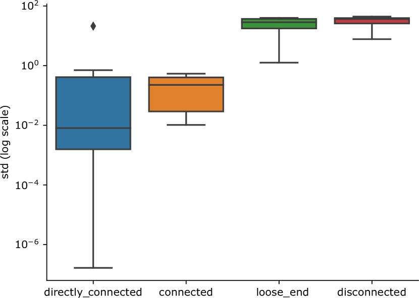
Figure 2: Educational example with four transitions and three states (state 0 is terminal). We characterize transitions based on the graph structure: (in-)directly connected to a terminal state (blue, orange); loose ends (green) and disconnected but infinite paths (red). The right plot illustrates the standard deviation over predicted Q-values for each type of transition from all 15 possible subsets of the educational example.

Confirming the finding in Van Hasselt et al. (2018), no unbounded divergence occurred (which would cause floating point NaNs). However, we found occurrences of soft divergence, i.e. Q-values beyond the realizable range as given by Eq. (missing) 1.
For further analysis we compute the standard deviation of Q-values that were estimated over different random seeds as a measure of soft divergence: if Q-learning for a transition converges, all Q-values should be identical and thus have a standard deviation close to zero. The more soft divergence occurs however, the larger the standard deviation becomes. Even if all trials diverge, it is highly unlikely that the resulting Q-values are identical.

Evaluating the distribution of standard variations reveals a link between the structure of the Q-graph and soft divergence:

1. Transitions $(s,a,r,s^{\prime},\mathfrak{t})$ where $s^{\prime}$ is terminal are referred to as directly connected. Their Q-values are estimated almost perfectly, because Q-learning is reduced to supervised learning in these cases (cf.  Eq. (missing) 4).

2. Transitions that end in a non-terminal state from which a terminal state is reachable are referred to as connected. Their Q-estimates exhibit only slightly more variance than the directly connected transitions. Presumably the reachable terminal state still acts as an anchor for the Q-value (as long as all transitions on the path are regularly used for updates). In line with this hypothesis, the two following categories that do not have an anchor show significantly more variance in their predictions:

3. If no terminal state is reachable from $s^{\prime}$ and there is no infinite path from $s^{\prime}$, the transition is referred to as a loose end. These transitions occur for instance at the end of each episode in episodic learning setups, when the agent does not succeed but is reset to a starting position. It is insightful to note that Q-values for such transitions are conceptually ill-defined in tabular Q-learning where a state without successors would be defined as terminal. For non-terminal states, a Q-value could be determined under the assumption that further transitions exist (and just have not been experienced yet), but then the Q-value is estimated using bootstrapping from another Q-value that has never been explicitly updated. This phenomenon is one example for what has been referred to as a lack of corrective feedback (Kumar et al., 2020). In other words, the estimate depends only on network initialization and generalization from data for other state-action pairs; cf. also Achiam et al. (2019) who analyze the theoretical link between approximator generalization properties and learning stability.

4. Transitions are referred to as disconnected if no terminal state is reachable from $s^{\prime}$ but there exists at least one infinite path from $s^{\prime}$. In applications of reinforcement learning, these transitions occur frequently, e.g. when the agent gets stuck in a non-terminal state.
   Disconnected transitions caused the highest variance in Q-estimates. In contrast to loose ends however, the Q-value for these transitions is well-defined under the assumption that all possible transitions are known and can even be computed analytically (cf.  Eq. (missing) 2).

We draw the following conclusions from this introductory experiment:

1. There is a clear link between the data graph structure and soft divergence; even for a static replay memory, a simple restricted policy and very few transitions.

2. Episodic tasks which create loose ends lead to an ill-posed estimation task which can only rely on generalization capabilities of the Q-function approximator.

3. Disconnected transitions pose a well-defined estimation problem and yet they cause the highest variance in Q-estimates in our experiment.

Our method, which will be presented in detail in the following section, extracts the largest possible subgraph for which exact Q-values can be computed under the assumption that all possible transitions are known. These Q-values represent a lower bound for the Q-value in the original continuous learning problem and enforcing them in temporal difference learning can stabilize learning. We will show empirically that, besides further effects, this reduces the variance of predicted Q-values also for a more realistic peg-in-hole continuous control task.

5 Q-graph bounded Q-learning

Building on the insights from Section 4, we select the largest set of transitions from the data graph for which exact Q-values can be computed under the assumption that the resulting graph is complete (i.e. that all possible transitions and all states are included). That is, we extract all transitions from the data graph except for loose ends. Formally, this induces a smaller finite MDP for which the associated Q-function can be computed using tabular Q-iteration with guaranteed convergence due to its contraction property. Our method is agnostic to the algorithm that computes these Q-values, so for instance it is also possible to solve the linear equation system for a sparse transition matrix. In any case, the computational overhead to compute these Q-values depends on the number of transitions in the replay memory, but it is independent of the input dimensionality. We annotate the subgraph of the data graph with the resulting Q-values and refer to it as Qgraph. One possible implementation of a Qgraph is illustrated in Algorithm 2 in Appendix A.

In many settings, there are known zero actions $a_{z}$ that do not change the agent’s state at all, e.g. moving by 0 units or applying 0 force. If those are applicable in all states, it may be possible to add a self-loop to every single node in the data graph. This effectively eliminates all loose ends and turns them into disconnected states, in other words it allows the Qgraph to contain all transitions from the data graph and compute their exact Q-values for the simplified MDP.

Qgraph Values as Lower Bounds

In general, the original MDP contains more states or transitions than the Qgraph. Then, the Q-values do not transfer to the original MDP as a correct solution but can be used as lower bounds for Q-values in the original MDP.

Assume w.l.o.g. that at least two transitions $(s_{0},a_{1},r_{1},s_{1})$ and $(s_{1},a_{2},r_{2},s_{2})$ are known and part of the Qgraph $\mathcal{G}$ with associated Q-values $\mathcal{Q}_{\mathcal{G}}$ for the associated simplified discrete MDP. Since Q-values for all transitions in $\mathcal{G}$ can be computed exactly using Q-iteration, the Bellman optimality equation applies:

$$\mathcal{Q}_{\mathcal{G}}(s_{0},a_{1})=r_{1}+\max_{a\in\mathcal{G}_{s_{1}}}\mathcal{Q}_{\mathcal{G}}(s_{1},a)$$ (6)

where $\mathcal{G}_{s_{1}}$ denotes all actions on out-going edges from $s_{1}$.

In the original MDP with potentially continuous state and action spaces, unseen states and transitions may exist. Still, in deterministic MDPs, the Q-value for the full MDP is lower bounded due to the $\max$ operation and the fact that the available actions in the Qgraph ($\mathcal{G}_{s_{1}}$) are a subset of those in the continuous action space $\mathcal{A}$:

$$\mathcal{Q}(s_{0},a_{1})= ~{}r_{1}+\max_{a\in\mathcal{A}}\mathcal{Q}(s_{1},a)$$ (7)

$$\geq ~{}r_{1}+\max_{a\in\mathcal{G}_{s_{1}}}\mathcal{Q}(s_{1},a)$$ (8)

$$= ~{}\mathcal{Q}_{\mathcal{G}}(s_{0},a_{1})$$ (9)

Thus, each Q-value for a transition in our Qgraph $\mathcal{G}$ represents a lower bound of the Q-value for the same transition in the original MDP on continuous state and action spaces. In contrast to the prior work in He et al. (2017), these lower bounds do not depend on the current Q-estimate but hold for the optimal Q-value in general.

Note that the $\max$ operation in Eq. (missing) 8 operates on a discrete space and can thus be computed by a simple look-up and comparison of all known transitions from $s_{1}$. To evaluate Eq. (missing) 7 in a continuous space, e.g. for temporal difference learning as in Eq. (missing) 4, the maximization is re-written using the currently estimate of the optimal policy $\pi^{*}_{Q}(s_{1})$:

$$\max_{a\in\mathcal{A}}\mathcal{Q}(s_{1},a)=\mathcal{Q}(s_{1},\pi^{*}_{\mathcal{Q}}(s_{1}))$$ (10)

In the DDPG setting and all our empirical evaluations, $\pi^{*}_{\mathcal{Q}}$ is represented by the actor network that is trained to maximize $\mathcal{Q}$.

For non-deterministic dynamics, potentially less tight bounds can be established under additional assumptions: If for any state and any series of actions $\mathfrak{A}$, the empirical return $R$ that an agent can observe when following $\mathfrak{A}$ from $s$ differs by at most $\delta$, then all Q-values from the simplified MDP apply as lower bounds with margin $\delta$:

$$\mathcal{Q}(s,a)\geq\mathcal{Q}_{\mathcal{G}}(s,a)-\delta$$ (11)

Since non-deterministic environments are quite common and $\delta$ may not be known, we will additionally evaluate the empirical performance of our method under violation of the determinism assumption.

Qgraph-bounded Q-learning

Bounds on Q-values, for instance those computed in Eq. (missing) 9, can be enforced in temporal difference learning by modifying target Q-values Eq. (missing) 4 as follows:

$$\mathcal{Q}_{\text{target}}(s_{t},a_{t})=\max\left(\text{LB}_{t},r_{t}+\begin{cases}0,&\text{if }s^{\prime}\text{ is terminal }\\ \gamma\cdot\mathcal{Q}(s_{t+1},\pi(s_{t+1})),&\text{else}\\ \end{cases}\right)$$ (12)

where LB_t is a lower bound; e.g. the Q-value for the same transition from the Qgraph $\mathcal{Q}_{\mathcal{G}}(s_{t},a_{t})$. If another lower bound is known, e.g. based on a bounded reward as in Eq. (missing) 1, LB can be the maximum over all available bounds. Analogously, upper bounds UB could be applied using the $\min$ operation.

We refer to this method of enforcing Q-values from $\mathcal{G}$ in the target values for temporal difference learning as Qgraph-bounded Q-learning. When the Q-function $\mathcal{Q}$ is represented by a function approximator, e.g. a neural network in DDPG, it is defined for a continuous state and action space. While training however, the Q-targets are constrained by bounds derived from the Qgraph-based $\mathcal{Q}_{\mathcal{G}}$-values on a discrete domain.

If a state-action pair is not associated with a lower bound, i.e. loose ends or transitions leading to such, can be used as usual in Eq. (missing) 4, i.e. without clipping of their target value. If coincidentally no bounds are violated, our method reduces to vanilla DDPG. A full training step is illustrated as pseudocode in Algorithm 1 in Appendix A.

6 Experimental Results

We evaluated the core of our method on a classical toy example for convergence issues in value learning in Section 6.1.

Additionally we ran a series of experiments on a continuous control problem (Section 6.2) to evaluate performance in terms of sample efficiency and robustness to hyperparameters in Section 6.3. In Section 6.4, we verify that the outcome on the continuous control problem is in line with the insights about soft divergence from our introductory example in Section 4. We further examine the impact of zero actions and different types of upper and lower bounds on Q-values (Section 6.5) as well as the method’s interaction with limited replay memory capacity (Section 6.6). Finally, we empirically asses the impact of non-deterministic transition dynamics in Section 6.7.

The usefulness of our method has further been demonstrated on an industrial insertion task in Hoppe et al. (2020).

6.1 Baird’s Star Problem

The 7-state star problem (Figure 3) was proposed by Baird (1999) to demonstrate convergence issues in value iteration with (linear) function approximation. The agent receives a reward of zero for each action and thus the correct solution to the problem is to set all weights to zero and obtain state-values of zero. If all weights are initially positive and $w_{0}$ larger than the others, this causes oscillatory behavior of both state values and weights. We reproduced the exact setting and result plots for Figure 4.2 in Baird (1999). Applying our graph view to the problem, we can derive a lower bound of zero for $V_{7}$ because it has a self-loop with reward 0; and thus this lower bound recursively leads to a lower bound of $0+\gamma V_{7}=0$ for all other states. These graph-based bounds can be applied in TD learning in analogy to Eq. (missing) 12 as $V^{\prime}(s)=\max(LB,r+\gamma V(s^{\prime}))$. As a result, our method converges to the correct state values rather than diverging to infinity as Figure 3 illustrates.

                   

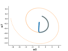
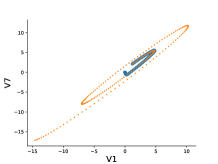
Figure 3: Graph-based bounds lead to the correct solution (blue, solid) on the 7-state star problem after Baird (1999), for which states and weights spiral out to infinity under vanilla TD learning (orange, dotted).

6.2 Experimental Setup

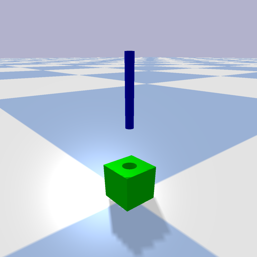
Figure 4: Simulated Peg-In-Hole task.

All further experiments were conducted on a simulated continuous control task. The environment was implemented using pybullet. A peg is supposed to be inserted into a green square object, see Figure 4. The peg is always upright and velocity-controlled: an action represents the three-dimensional offset to the next position. The simulation is stepped forward until a stable new position is reached. The actions are box-constrained to $[-1,1]$ in each dimension which corresponds to a movement of 1cm. The green object has a width of 5cm and is within a cubic state space of width 20cm. The peg has a diameter of 1cm, the hole’s diameter is 2cm. The agent receives a distance-based reward $r=\exp(-\frac{\Delta}{0.03})-1$, where $\Delta$ is the Euclidean distance to the goal position in meters.

We use the following instance of a standard DDPG architecture for learning: The critic network consists of three fully connected layers with 200 nodes each. For the inner layers, ReLU activations were used. The network was initialized with weights sampled from $\mathcal{N}(\mu=0,\sigma=0.001)$. The actor network also consists of three fully connected layers with 200 nodes each, but used tanh activations and was initialized from a He-uniform distribution. All neural networks were implemented using Tensorflow and optimized using the AdamOptimizer, with 50 training epochs after each episode (i.e. 200 agent steps) and up to 15 random mini batches of data per epoch. No target network was used, since those are known to prolong training and thereby postpone convergence issues but not solve them (Van Hasselt et al., 2018).

We tested vanilla DDPG for 300 episodes on a grid of learning rates for actor and critic in $\{10^{-2},10^{-3},10^{-4}\}$ and chose three sets of hyperparameters for the following experiments that are representative for the spectrum of DDPG performance, see Figure 5.

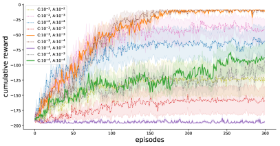
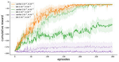
Figure 5: Performance of vanilla DDPG on the full grid of learning rates (left). Three representative parameters were identified (solid lines) and compared to our method (’QG’, dotted lines) on the right plot.

In all plots with learning curves, the line represents the mean performance over ten runs with different random seeds and the shaded area highlights the standard deviation of the mean estimator, i.e. $\frac{\sigma}{\sqrt{n}}$.

6.3 Sample Efficiency and Robustness to Hyperparameters

We hypothesized that Qgraph-based lower bounds would correctly limit the range of Q-values which prevents some cases of soft divergence and thereby increases sample efficiency. We further hypothesized that explicit bounds would barely have any impact in cases when vanilla Q-learning works well, because our method as described in Eq. (missing) 12 reduces to standard TD learning when no bound is violated. In other words this implies that Qgraph-bounded Q-learning should never decrease performance.
For a first overview, we compared learning curves of Qgraph-bounded Q-learning (’QG’) to those of vanilla DDPG in Figure 5. As expected, Qgraphs speed up learning for all examined learning rates. The effect size varies and is larger for those learning rates that lead to relatively poor performance in vanilla DDPG. This decreases the gap in performance between different learning rates and can therefore be interpreted as an indicator for increased robustness to hyperparameters.

6.4 Variance of Predictions

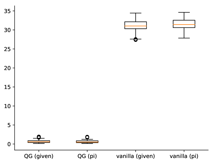
Figure 6: Standard deviation of predicted Q-values.

To assess if this increase in performance is due to similar effects as in our educational examples, we evaluated the variance in predicted Q-values at the end of each experiment under the learning rate with largest effect size ($10^{-4}$). We covered the state space with a regular grid of 27 states and evaluated the learned Q-value for each of these states with a set of eleven given actions (’given’) as well as with the action that the actor network suggests for each state (’pi’).
For the boxplot in Figure 6, we collected the standard deviations over the predicted Q-values for each state-action pair from 10 runs with different random seeds. The orange line indicates the median value, the box extends from the lower to the upper quartile value, the whiskers cover 1.5 times the inter quartile range and outliers are shown as circles. The results shows very clearly that Qgraph-runs resulted in significantly less variance for predicted Q-values, indicating that Qgraph-bounded Q-learning does indeed prevent cases of soft divergence.

6.5 Further Baselines

We ran the following baselines to deepen our understanding of the previously reported effects: In many settings a zero action is known that does not change the agent’s state (in our case it is the offset in position by zero meters). Adding hypothetical transitions with the zero action after each physical transition (’vanilla-ZA’) improves the structure of the data graph by turning loose ends into disconnected transitions. Using zero actions in our method (’QG-ZA’) not only improves the structure of the data graph but also spreads information in the form of lower bounds to predecessors in the Qgraph.
The results are shown in Figure 7. Adding zero actions to vanilla DDPG does lead to an improvement, even without any Qgraph-bounded learning. This supports the importance of the data graph structure for Q-learning in general. Also our method can be slightly improved by adding zero actions, but the largest performance gap is still between vanilla-ZA and our method. This indicates that while the data graph structure matters, the propagation of information through the Qgraph and the integration of lower bounds into TD-learning are the main causes for benefits from our method.

Figure 7: Zero Actions (ZA, left) eliminate loose ends; trivial bounds are evaluated as baselines to our Qgraph-based bounds on the right.

The next set of baselines was designed to evaluate how much influence the exact bounds have. Bounded temporal difference learning could, besides our Qgraph-based bounds, integrate two further types of lower and upper bounds: A priori bounds may be known in the case of a bounded reward function, see Eq. (missing) 1. Empirical bounds may seem like an alternative for correct a priori bounds: rather than using known bounds on the reward, these bounds could be estimated from experience. For the experiment, we used the lowest observed and highest observed rewards to compute bounds using Eq. (missing) 1. Note that the true Q-values are guaranteed to lie within Qgraph-based bounds and correct a priori bounds, while empirical bounds might be too tight. We combined Qgraph-bounded Q-learning and vanilla DDPG with both types of bounds. When several bounds were available for one Q-value, the tightest upper and lower bound were chosen. The results in Figure 7 confirm that incorrect empirical bounds (green lines) have adverse effects on both methods, while a priori bounds do not seem to have any significant effect. In particular, adding an upper a priori bound does not have a significant effect on our method. We hypothesize that this may also be because the behavior of a Q-learning system differs for under- and over-estimated states: while under-estimated states may just never be visited (or rarely, depending on the type of exploration), over-estimated states are likely to be visited using the currently estimated optimal policy. Therefore, lower bounds correcting under-estimated states may be more important than upper bounds which would correct over-estimated states. Overall, we conclude that the tight sample-specific lower bounds from our Qgraph are key and much more informative than more general bounds.

6.6 Limited Graph Capacity

In deep reinforcement learning, the replay memory is typically a FIFO-buffer (’first in, first out’), i.e. those elements that were added first are overwritten first when the buffer is full. For a data graph, it is possible to delete single transitions but there are two possible effects: On the one hand, some information from deleted transitions can be implicitly contained in its predecessors’ Q-values on the Qgraph, which could imply that our method is more robust to small memory capacities. On the other hand, cuts from deleted transitions can stop information propagation through the Qgraph, which could in turn slow down further progress.

We therefore empirically compared the drop in performance for vanilla DDPG and our Qgraph-bounded Q-learning with graph capacities of 1000 and 5000 transitions. For comparison, the average unlimited graph contained roughly 30,000 unique transitions at the end of our 300 episode experiments. As Figure 8 illustrates, a Qgraph-based method that is limited to only 1000 samples still performs on par with unlimited vanilla DDPG, while the vanilla DDPG performance decreases for a limit of 1000 transitions.

6.7 Non-Deterministic Transitions

As discussed in Section 5, the Qgraph-derived lower bounds are based on the assumption that all transitions are deterministic. In case of non-deterministic transitions, correct lower bounds can be derived if for any state and any series of actions $\mathfrak{A}$, the empirical return $R$ that an agent can observe when following $\mathfrak{A}$ from $s$ differs by at most $\delta$. In practice however, $\delta$ may not exist or be unknown. We therefore empirically compare the results from Section 6.3 with increasing amounts of transition uncertainty. To obtain the results shown in Figure 8, each action was sampled from a Gaussian around the actor output with different $\sigma$: $\mathcal{N}(\pi(s),\sigma)$. The results show that the performance generally drops with non-determinism for all methods, but the improvement of Qgraph-bounded Q-learning over vanilla DDPG remains significant.

Figure 8: Performance with limited graph capacity (left) and increasingly non-deterministic transitions (right).

7 Conclusion

From the observation that even for continuous state and action spaces, model-free off-policy deep reinforcement learning algorithms perform network updates on a finite set of transitions, we have developed a graph perspective on the replay memory that allows closer analysis. Two types of data graph structures are clearly linked to soft divergence: non-terminal states without successors (loose ends) and infinite loops with no path to a terminal state (disconnected states).

Our method constructs a simplified MDP from a subgraph such that its exact Q-values can be computed by Q-iteration – resulting in a Qgraph. This subgraph does not contain loose ends, but we introduce so-called zero actions which, if known, can be used to integrate loose ends into the Qgraph as well.
Q-values on the discrete simplified MDP associated with the Qgraph represent lower bounds for the Q-values in the original continuous MDP. Enforcing these bounds in TD-learning empirically prevents cases of soft divergence on a continuous control task.

Preventing soft divergence as our method does, also increases sample efficiency on average and leads to the largest effect for unfavorable hyperparameters; i.e. our method increases robustness to adverse hyperparameters. We have also demonstrated that the Qgraph can serve as an additional implicit memory holding information from transitions that have already been overwritten in the replay memory and thus, the algorithm is able to cope better with restricted memory capacity. Empirically, the method also works in non-deterministic settings despite being derived under the assumption of deterministic transitions.

This work gives rise to a number of questions for future work: (1) further bounds may exist, including data-driven or heuristic upper bounds; (2) the reward function most likely interacts with soft divergence and thus it may be possible to derive implications for reward shaping from our method; (3) exploration may benefit from current graph structure information; (4) there may be further application-specific methods to integrate loose ends into the Qgraph structure, e.g. querying expert demonstrations.

Appendix A PseudoCode

Algorithm 1 describes the core of Qgraph-bounded Q-learning: one update step including the graph-based lower bounds, which were obtained from a Qgraph $\mathcal{G}$. One possible implementation of a Qgraph which is iteratively constructed as new data comes in, is provided in Algorithm 2.

Algorithm 1 Qgraph-bounded DDPG

1:procedure trainStep( discount factor $\gamma$, actor network $\pi$, $\triangleright$ mapping states to actions critic network $\mathcal{Q}$, $\triangleright$ predicting Q-values for state-action pairs Qgraph $\mathcal{G}$, $\triangleright$ see Algorithm 2 a priori lower bound $\text{LB}^{AP}$, $\triangleright$ A priori lower bound on Q-values if known. else $-\infty$ a priori upper bound $\text{UB}^{AP}$ )$\triangleright$ A priori upper bound on Q-values if known. else $+\infty$

2:

3:     sample minibatch of $N$ transitions ${(s_{i},a_{i},s_{i}^{\prime},r_{i},t_{i},\text{LB}_{i}^{\mathcal{G}})}_{i=0}^{N}$ from $\mathcal{G}$ $\triangleright$ unknown lower bounds set to $-\infty$

4:     $Q_{\text{target}}(s_{i},a_{i})=\begin{cases}r_{i},&\text{if }s_{i}^{\prime}\text{ is terminal (t)}\\ r_{i}+\gamma\cdot\mathcal{Q}(s_{i}^{\prime},\pi(s_{i}^{\prime})),&\text{else}\\ \end{cases}$ $\triangleright$ classical Q targets, see Eq. (missing) 4

5:     $\text{LB}_{i}=\text{max}(\text{LB}_{i}^{\mathcal{G}},\text{LB}_{i}^{AP})$ $\triangleright$ tightest available lower bound

6:     $Q_{\text{target}}^{B}(s_{i},a_{i})=\text{min}(\text{UB}_{i}^{AP},\text{max}(\text{LB}_{i},Q_{\text{target}}(s_{i},a_{i})))$ $\triangleright$ apply bounds, see Eq. (missing) 12

7:     $\mathcal{L}_{C}=\frac{1}{N}\sum_{i=0}^{N}(Q_{\text{target}}^{B}(s_{i},a_{i})-\mathcal{Q}(s_{i},a_{i}))^{2}$ $\triangleright$ DDPG Critic Loss, see Eq. (missing) 5

8:     $\mathcal{L}_{A}=-\frac{1}{N}\sum_{i=0}^{N}\mathcal{Q}(s_{i},\pi(s_{i}))$ $\triangleright$ DDPG Actor Loss

9:     optimization step for both networks using $\mathcal{L}_{A}$ and $\mathcal{L}_{C}$

10:end procedure

Algorithm 2 Graph

1:  successors = {} $\triangleright$ maps state $s$ to list of tuples ($s^{\prime}$, $a$, $r$, $t$, LB_Q) predecessors = {} $\triangleright$ maps state $s^{\prime}$ to list of tuples ($a$, $r$, $s$) discount factor $\gamma$ zero action ZA, if known capacity $\mathcal{C}$ $\triangleright$ max. number of transitions to store

2:

3:procedure addTransition($s$, $a$, $s^{\prime}$, $r$, $\mathfrak{t}$)

4:     add ($a$, $r$, $s$) to predecessors[$s^{\prime}$] unless already exists

5:     LB$=$LBforNewTransition($s$, $a$, $r$, $s^{\prime}$, $\mathfrak{t}$)

6:     add ($s^{\prime}$, $a$, $r$, $\mathfrak{t}$, LB) to successors[$s$] unless already exists

7:     if LB $\neq$ NaN then

8:         propagateLB($s$) $\triangleright$ Update predecessor bounds

9:     end if

10:     if capacity $\mathcal{C}$ reached then

11:         remove transition $\triangleright$ e.g. first-in-first-out (FIFO)

12:     end if

13:     if Zero Action ZA known and $\mathfrak{t}=0$ and $s\neq s^{\prime}$ then

14:         addTransition($s^{\prime}$, ZA, $s^{\prime}$, $\frac{r}{1-\gamma}$, $\mathfrak{t}=0$)

15:     end if

16:end procedure

17:

18:function LBforNewTransition($s$, $a$, $r$, $s^{\prime}$, $\mathfrak{t}$)

19:     $\text{LB}=\text{{NaN}}$ $\triangleright$ lower bound unknown so far

20:     if $\mathfrak{t}$ then $\triangleright$ $s^{\prime}$ is terminal state

21:         $\text{LB}=\max(\text{LB},r)$

22:     end if

23:     if $s$ = $s^{\prime}$ then $\triangleright$ self-loop, e.g. zero action

24:         $\text{LB}=\max(\text{LB},\frac{r}{1-\gamma})$

25:     end if

26:     if larger loop with n transitions from $s$ detected then

27:         $\text{LB}=\max(\text{LB},\frac{r_{L}}{1-\gamma^{n}})$ $\triangleright$ see Eq. (missing) 2

28:     end if

29:     if there are successor transitions from $s^{\prime}$ with a lower bound then

30:         $\text{LB}=\max(\text{LB},r+\gamma\cdot\max\{\text{lower bound LB' for transitions in successors[$s^{\prime}$]}\})$

31:     end if

32:     return LB $\triangleright$ tightest lower bound

33:end function

34:

35:procedure propagateLB(start_state)

36:     S = [start_state] $\triangleright$ list of states to visit

37:     while states in S do

38:         s = S.pop(0) $\triangleright$ remove and obtain first element in S

39:         if s has predecessors and successors then

40:              LB${}^{\prime}=\max\{\text{lower bounds LB' for transitions in successors[$s$]}\}$

41:              for ps in predecessors[$s$] do $\triangleright$ iterate predecessors of $s$

42:                  LB${}_{2}=r^{\text{ps}}_{s}+\gamma\cdot\text{LB}^{\prime}$ $\triangleright$ $r^{\text{ps}}_{s}$: reward for transition ps $\rightarrow$ s

43:                  if LB${}_{2}>$ existing bound for ps $\rightarrow$ s then

44:                       update LB in transition ps $\rightarrow$ s

45:                       S.add(ps)

46:                  end if

47:              end for

48:         end if

49:     end while

50:end procedure

51:

References

- Achiam et al. [2019] J. Achiam, E. Knight, and P. Abbeel. Towards characterizing divergence in deep q-learning. arXiv preprint arXiv:1903.08894, 2019.
- Amiranashvili et al. [2018] A. Amiranashvili, A. Dosovitskiy, V. Koltun, and T. Brox. Analyzing the role of temporal differencing in deep reinforcement learning. In ICLR, 2018. URL https://openreview.net/forum?id=HyiAuyb0b.
- Anschel et al. [2017] O. Anschel, N. Baram, and N. Shimkin. Averaged-dqn: Variance reduction and stabilization for deep reinforcement learning. In ICML, pages 176–185, 2017.
- Baird [1995] L. Baird. Residual algorithms: Reinforcement learning with function approximation. In Machine Learning Proceedings 1995, pages 30–37. Elsevier, 1995.
- Baird [1999] L. C. Baird. Reinforcement learning through gradient descent. PhD thesis, Carnegie Mellon University, 1999. URL http://reports-archive.adm.cs.cmu.edu/anon/1999/CMU-CS-99-132.pdf.
- Blundell et al. [2016] C. Blundell, B. Uria, A. Pritzel, Y. Li, A. Ruderman, J. Z. Leibo, J. Rae, D. Wierstra, and D. Hassabis. Model-free episodic control. arXiv preprint arXiv:1606.04460, 2016.
- Corneil et al. [2018] D. Corneil, W. Gerstner, and J. Brea. Efficient model-based deep reinforcement learning with variational state tabulation. In ICML, pages 1049–1058, 2018.
- De Asis et al. [2019] K. De Asis, A. Chan, S. Pitis, R. S. Sutton, and D. Graves. Fixed-horizon temporal difference methods for stable reinforcement learning. arXiv preprint arXiv:1909.03906, 2019.
- Degris et al. [2012] T. Degris, M. White, and R. S. Sutton. Off-policy actor-critic. In ICML, pages 179–186, 2012.
- Durugkar and Stone [2018] I. Durugkar and P. Stone. TD learning with constrained gradients, 2018. URL https://openreview.net/forum?id=Bk-ofQZRb.
- Fazeli et al. [2017] N. Fazeli, S. Zapolsky, E. Drumwright, and A. Rodriguez. Learning data-efficient rigid-body contact models: Case study of planar impact. In CoRL, pages 388–397, 2017.
- Fedus et al. [2020] W. Fedus, P. Ramachandran, R. Agarwal, Y. Bengio, H. Larochelle, M. Rowland, and W. Dabney. Revisiting fundamentals of experience replay. In ICML, 2020.
- Fu et al. [2019] J. Fu, A. Kumar, M. Soh, and S. Levine. Diagnosing bottlenecks in deep q-learning algorithms. In ICML, pages 2021–2030, 2019.
- Fujimoto et al. [2018] S. Fujimoto, H. van Hoof, and D. Meger. Addressing function approximation error in actor-critic methods. Proceedings of Machine Learning Research, 80:1587–1596, 2018.
- Fujimoto et al. [2019] S. Fujimoto, D. Meger, and D. Precup. Off-policy deep reinforcement learning without exploration. In ICML, pages 2052–2062, 2019.
- Ghiassian et al. [2018] S. Ghiassian, A. Patterson, M. White, R. S. Sutton, and A. White. Online off-policy prediction. arXiv preprint arXiv:1811.02597, 2018.
- Gu et al. [2017] S. S. Gu, T. Lillicrap, R. E. Turner, Z. Ghahramani, B. Schölkopf, and S. Levine. Interpolated policy gradient: Merging on-policy and off-policy gradient estimation for deep reinforcement learning. In NeurIPS, pages 3846–3855, 2017.
- He et al. [2017] F. S. He, Y. Liu, A. G. Schwing, and J. Peng. Learning to play in a day: Faster deep reinforcement learning by optimality tightening. In ICLR, 2017.
- Henderson et al. [2018] P. Henderson, R. Islam, P. Bachman, J. Pineau, D. Precup, and D. Meger. Deep reinforcement learning that matters. In AAAI, 2018.
- Hernandez-Garcia and Sutton [2019] J. F. Hernandez-Garcia and R. S. Sutton. Understanding multi-step deep reinforcement learning: A systematic study of the dqn target. arXiv preprint arXiv:1901.07510, 2019.
- Hoppe et al. [2020] S. Hoppe, M. Giftthaler, R. Krug, and M. Toussaint. Sample-efficient learning for industrial assembly using qgraph-bounded ddpg. In IROS, 2020.
- Kumar et al. [2019] A. Kumar, J. Fu, M. Soh, G. Tucker, and S. Levine. Stabilizing off-policy q-learning via bootstrapping error reduction. In NeurIPS, pages 11784–11794, 2019.
- Kumar et al. [2020] A. Kumar, A. Gupta, and S. Levine. Discor: Corrective feedback in reinforcement learning via distribution correction. arXiv preprint arXiv:2003.07305, 2020.
- Lee and Kim [2015] K. Lee and K.-E. Kim. Tighter value function bounds for bayesian reinforcement learning. In AAAI, 2015.
- Lee et al. [2019] S. Y. Lee, C. Sungik, and S.-Y. Chung. Sample-efficient deep reinforcement learning via episodic backward update. In NeurIPS, pages 2112–2121, 2019.
- Levine et al. [2016] S. Levine, P. Pastor, A. Krizhevsky, and D. Quillen. Learning hand-eye coordination for robotic grasping with deep learning and large-scale data collection. CoRR, abs/1603.02199, 2016.
- Lillicrap et al. [2015] T. P. Lillicrap, J. J. Hunt, A. Pritzel, N. Heess, T. Erez, Y. Tassa, D. Silver, and D. Wierstra. Continuous control with deep reinforcement learning. arXiv preprint arXiv:1509.02971, 2015.
- Mnih et al. [2015] V. Mnih, K. Kavukcuoglu, D. Silver, A. A. Rusu, J. Veness, M. G. Bellemare, A. Graves, M. Riedmiller, A. K. Fidjeland, G. Ostrovski, et al. Human-level control through deep reinforcement learning. Nature, 518(7540):529, 2015.
- Mnih et al. [2016] V. Mnih, A. P. Badia, M. Mirza, A. Graves, T. Lillicrap, T. Harley, D. Silver, and K. Kavukcuoglu. Asynchronous methods for deep reinforcement learning. In ICML, pages 1928–1937, 2016.
- Munos et al. [2016] R. Munos, T. Stepleton, A. Harutyunyan, and M. Bellemare. Safe and efficient off-policy reinforcement learning. In NeurIPS, pages 1054–1062, 2016.
- Ohnishi et al. [2019] S. Ohnishi, E. Uchibe, K. Nakanishi, and S. Ishii. Constrained deep q-learning gradually approaching ordinary q-learning. Frontiers in neurorobotics, 13:103, 2019.
- Precup et al. [2000] D. Precup, R. S. Sutton, and S. Singh. Eligibility traces for off-policy policy evaluation. In ICML, 2000.
- Silver et al. [2017] D. Silver, J. Schrittwieser, K. Simonyan, I. Antonoglou, A. Huang, A. Guez, T. Hubert, L. Baker, M. Lai, A. Bolton, et al. Mastering the game of go without human knowledge. Nature, 550(7676):354, 2017.
- Sutton and Barto [2018] R. S. Sutton and A. G. Barto. Reinforcement learning: An introduction. MIT press, 2018.
- Tang [2020] Y. Tang. Self-imitation learning via generalized lower bound q-learning. arXiv preprint arXiv:2006.07442, 2020.
- Touati et al. [2020] A. Touati, A. Zhang, J. Pineau, and P. Vincent. Stable policy optimization via off-policy divergence regularization. arXiv preprint arXiv:2003.04108, 2020.
- Van Hasselt et al. [2016] H. Van Hasselt, A. Guez, and D. Silver. Deep reinforcement learning with double q-learning. In AAAI, 2016.
- Van Hasselt et al. [2018] H. Van Hasselt, Y. Doron, F. Strub, M. Hessel, N. Sonnerat, and J. Modayil. Deep reinforcement learning and the deadly triad. arXiv preprint arXiv:1812.02648, 2018.
- Zhang et al. [2019] Z. Zhang, J. Chen, Z. Chen, and W. Li. Asynchronous episodic deep deterministic policy gradient: Toward continuous control in computationally complex environments. IEEE Transactions on Cybernetics, 2019.
- Zhu et al. [2019] G. Zhu, Z. Lin, G. Yang, and C. Zhang. Episodic reinforcement learning with associative memory. In ICLR, 2019.