Excitation Energies from Thermally-Assisted-Occupation Density Functional Theory: Theory and Computational Implementation

Abstract

The time-dependent density functional theory (TDDFT) has been broadly used to investigate the excited-state properties of various molecular systems. However, the current TDDFT heavily relies on outcomes from the corresponding ground-state density functional theory (DFT) calculations which may be prone to errors due to the lack of proper treatment in the non-dynamical correlation effects. Recently, thermally-assisted-occupation density functional theory (TAO-DFT) [J.-D. Chai, J. Chem. Phys. 136, 154104 (2012)], a DFT with fractional orbital occupations, was proposed, explicitly incorporating the non-dynamical correlation effects in the ground-state calculations with low computational complexity. In this work, we develop time-dependent (TD) TAO-DFT, which is a time-dependent, linear-response theory for excited states within the framework of TAO-DFT. With tests on the excited states of H₂, the first triplet excited state ($1^{3}\Sigma_{u}^{+}$) was described well, with non-imaginary excitation energies. TDTAO-DFT also yields zero singlet-triplet gap in the dissociation limit, for the ground singlet ($1^{1}\Sigma_{g}^{+}$) and the first triplet state ($1^{3}\Sigma_{u}^{+}$). In addition, as compared to traditional TDDFT, the overall excited-state potential energy surfaces obtained from TDTAO-DFT are generally improved and better agree with results from the equation-of-motion coupled-cluster singles and doubles (EOM-CCSD).

I Introduction

Over the past decades, Kohn-Sham density functional theory (KS-DFT) Hohenberg and Kohn (1964); Kohn and Sham (1965) has been extensively used in the prediction of various ground-state properties of solids as well as finite-sized molecules. Jones (2015); Becke (2014); Mardirossian and Head-Gordon (2017) Its time-dependent (TD) extension, known as TDDFT Runge and Gross (1984); Petersilka et al. (1996); Casida (1995), has been a popular approach for computing excited-state properties, including the absorption and emission spectra Dreuw and Head-Gordon (2005), photochemical reactions Deskevich et al. (2006), dynamics Tavernelli et al. (2005), energy and electron transfer Toivonen et al. (2006), etc., due to its low computational cost and the availability of a plethora of computer codes in this area. The one-to-one correspondence between the TD density and the TD external potential was rigorously demonstrated by Runge and Gross in 1984 in their theorem Runge and Gross (1984). The linear-response framework was further introduced  Petersilka et al. (1996); Casida (1995), which brought forth a paradigm shift in the simulation of excitations of quantum systems from a density-functional perspectiveHirata and Head-Gordon (1999); Stratmann et al. (1998); Hsu et al. (2001) and is the main reason behind the popularity of this method.

However, conventional TDDFT is derived from ground-state (GS) KS-DFT which is a single-determinant–based method. As a result, it can fail to describe the excited-state phenomena heavily governed by non-dynamical (or static) correlation, such as photochemistry processes involving photoinduced bond breaking, and problems associated with conical intersection Petersilka et al. (1996); Dreuw and Head-Gordon (2005); Levine et al. (2006); Filatov (2013). A prototypical example is the bond dissociation process of the H₂ molecule. It is known that the excitation energy of the lowest triplet state of H2, computed using conventional TDDFT Dreuw and Head-Gordon (2005), would become imaginary beyond a H-H bond distance of 1.75 Å, a phenomenon arising from a spin symmetry-breaking solution in the ground state Gritsenko et al. (2000); Casida et al. (2000), a typical characteristic of nondynamical correlation effects. In contrast, in wavefunction-based methods, the (nearly) degenerate determinants are considered on an equal footing when performing a self-consistent field (SCF) calculation, and this is the basis of multi-configuration (MC) SCF or complete active space (CAS) SCF-based methodologies. However, these methods can be prohibitively expensive for large systems, as their computational cost scales factorially with the size of active space.

KS-DFT with proper exchange energy functionals may reasonably model systems with non-dynamical correlation, albeit at the expense of enormous computation efforts. For example, the works by Becke Becke (2005, 2013) and the works by Kong and coworkers Proynov et al. (2010, 2012); Kong and Proynov (2016) demonstrated parametric functionals which need to be solved self-consistently within the single-determinant framework. Although these works significantly improved the bond dissociation trends of simple diatomic molecules, compared to the Hartree-Fock theory, they still deviate appreciably at the bond dissociation limit compared to a full configuration interaction (FCI) calculation Proynov et al. (2010, 2012). Moreover, the SCF associated with these functionals adds to the computational effort which can scale dramatically with the size of molecules.

On the other hand, various approaches have been developed to cope with the non-dynamical correlation effects without the high computational cost of an exact exchange functional. The CAS-DFT model is one such method Gräfenstein and Cremer (2000), wherein some amount of correlation has been accounted for, by a density functional calculation. As a result, the dynamical correlation associated with the MC representation of the system might be “double counted” Li Manni et al. (2014, 2016). To mitigate this issue, the multi-configuration pair-density functional theory Li Manni et al. (2014, 2016) and multi-configuration range-separated DFT Fromager et al. (2013); Sharkas et al. (2012) were developed. While the former utilizes the so-called on-top pair-density functional, the latter separates the electron interaction operator into short- and long-range parts which are treated with DFT and wavefunction theory, respectively. Although the idea of using such a “hybrid” scheme seems to be an attractive prospect Li Manni et al. (2014, 2016); Fromager et al. (2013); Sharkas et al. (2012), they can be computationally demanding for increasing system sizes because of the initial generation of MC wavefunctions.

Another category of computational methods exists, which can cope with non-dynamical correlation with the additional advantage that they are low-cost methods. They include the spin-flip, ionization-potential, and electron-affinity based approaches which are aimed to start with a high-spin, with 1-less or 1-more electron single-determinant references such that the non-dynamical correlation problem is minimal Stanton and Gauss (1994); Nooijen and Bartlett (1998); Shao et al. (2003). These approaches require a well-balanced treatment of the orbitals in the reference, and they can offer high-quality solutions in many cases. However, the requirement of balanced treatment of orbitals in the reference is not always feasible, and thus applications are limited.

In this regard, the thermally-assisted-occupation density functional theory (TAO-DFT) Chai (2012) was developed by Chai in 2012 to alleviate the formidable challenge of balancing the computational cost and simultaneously incorporating the non-dynamical correlation effects with reasonable accuracy. In contrast to traditional KS-DFT, the underlying principle of TAO-DFT is in the usage of fractional orbital occupations according to a given fictitious temperature ($\theta$), to effectively incorporate the different electronic configurations of a system. This approach ensures that some “excitations” in the form of fractional populations of electrons in the low-lying virtual orbitals are considered along with the GS of the system, similar to a multi-determinant expansion of the wavefunction. The inclusion of fractional occupancies is a computationally cheaper alternative to a multi-determinant expansion for accounting non-dynamical correlation effects. As a result, TAO-DFT has a computational cost similar to that of KS-DFT, which is $\mathcal{O}(N^{3\text{-}4})$. In TAO-DFT, the entropy contribution (e.g., see Eq. (26) of Ref.33), can reasonably capture the non-dynamical correlation energy of a system, which was discussed and numerically investigated in Ref. 33, even when the simplest local density approximation (LDA) XC energy functional is used. The XC energy functionals at the higher rungs of Jacob’s ladder, such as the generalized-gradient approximation (GGA) Chai (2014), global hybrid Chai (2017), and range-separated hybrid Chai (2017); Xuan et al. (2019) XC energy functionals, can also be employed in TAO-DFT. Moreover, a self-consistent scheme that determines the fictitious temperature in TAO-DFT has been recently proposed to improve the performance of TAO-DFT for a wide range of applications Lin et al. (2017). Since TAO-DFT is similar to KS-DFT in computational efficiency, TAO-DFT has been recently adopted for the study of the electronic properties of various nanosystems with pronounced radical nature Xuan et al. (2019); Wu and Chai (2015); Yeh and Chai (2016); Seenithurai and Chai (2016); Wu et al. (2016); Seenithurai and Chai (2017, 2018); Yeh et al. (2018); Chung and Chai (2019). In particular, the electronic properties (e.g., singlet-triplet energy gaps, vertical ionization potentials, vertical electron affinities, fundamental gaps, and active orbital occupation numbers) of linear acenes and zigzag graphene nanoribbons (i.e., systems with polyradical character) obtained from TAO-DFT Chai (2012, 2014, 2017); Wu and Chai (2015) have been shown to be in reasonably good agreement with those obtained from other accurate electronic structure methods, such as the particle-particle random-phase approximation (pp-RPA) Yang et al. (2016) XC energy functional in KS-DFT, the density matrix renormalization group (DMRG) algorithm Hachmann et al. (2007); Mizukami et al. (2013), the variational two-electron reduced density matrix (2-RDM) method Pelzer et al. (2011); Fosso-Tande et al. (2016), and other high-level methods Deleuze et al. (2003); Hajgato et al. (2008, 2009, 2011).

II Ground-state reference: TAO-DFT

In TAO-DFT Chai (2012), the electron density is represented by the thermal equilibrium density of an auxiliary system of $N_{\mathrm{e}}$ non-interacting electrons at a fictitious temperature $\theta$ (in energy units):

$$\rho(\mathbf{r})=\sum_{i}f_{i}\,\phi^{*}_{i}(\mathbf{r})\phi_{i}(\mathbf{r}).$$ (1)

Here, $f_{i}$ (a value between 0 and 1) is the fractional occupation number of the $i^{\text{th}}$ orbital $\phi_{i}$, and is given by the Fermi-Dirac distribution function

$$f_{i}=\Big{\{}1+\exp\big{[}(\varepsilon_{i}-\mu)/\theta\big{]}\Big{\}}^{-1},$$ (2)

where $\mu$ is the chemical potential for electrons, and is determined by $\sum_{i}f_{i}=N_{\mathrm{e}}$ for a given $\theta$, orbital energies $\{\varepsilon_{i}\}$, and total electron number $N_{\mathrm{e}}$. This choice for the fractional occupation function and the corresponding one-particle density matrix has been extensively used in other methods such as finite-temperature DFT (FT-DFT) Mermin (1965) and floating occupation molecular orbital-complete active space configuration interaction (FOMO-CASCI) Slavíček and Martínez (2010). With this assisted occupation number and generalized density expression, the total ground-state energy functional can be written as

$$E_{\text{G}}[\rho]=T_{\text{TAO}[\{f_{i},\phi_{i}\}]}+V_{\text{ext}}[\rho]+E_{\text{Hxc}}^{\text{KS}}+E_{\theta}[\rho],$$ (3)

where $T_{\textrm{TAO}}$ is the kinetic free energy functional of non-interacting electrons (equivalent to $A_{s}^{\theta}$ as defined in Eq. (24) of Ref. 33), $V_{\text{ext}}[\rho]$ is the energy functional of the external potential (or nuclei potential), $E_{\text{Hxc}}^{\text{KS}}$ is the sum of Hartree and XC energy functionals in KS-DFT, and $E_{\theta}$ is the $\theta$-dependent energy functional Chai (2012). Alternatively (to the original derivation Chai (2012)), from Eq. 3, upon performing the functional derivatives with respect to the orbitals ($\phi_{i}$), we can also obtain the SCF equations in TAO-DFT:

$$\bigg{[}-\frac{1}{2}\nabla_{\mathbf{r}}^{2}+v_{\text{ext}}(\mathbf{r})+v_{\text{Hxc}}^{\text{KS}}(\mathbf{r})+v_{\theta}(\mathbf{r})\bigg{]}\phi_{i}(\mathbf{r})=\varepsilon_{i}\phi_{i}(\mathbf{r}),$$ (4)

where $v_{\text{ext}}$, $v_{\text{Hxc}}^{\text{KS}}$, and $v_{\theta}$ are the potentials (or functional derivatives) of corresponding energy functionals (i.e., $V_{\text{ext}}[\rho]$, $E_{\text{Hxc}}^{\text{KS}}$, and $E_{\theta}[\rho]$, respectively) in Eq. 3, and $\{\phi_{i}\}$ and $\{\varepsilon_{i}\}$ are the TAO orbitals and orbital energies, respectively, which can be solved self-consistently through SCF. The algorithm is similar to KS-DFT, with the only differences being the $v_{\theta}(\mathbf{r})$ term in the Hamiltonian and the determination of chemical potential $\mu$, making this approach attractive and easy in implementation. We have provided a variational perspective of TAO-DFT in Appendix A, which complements the derivation in Ref. 33.

III Excited state theory: TDTAO-DFT

III.1 Mathematical Formalism

In the present work, we propose TDTAO-DFT, which is a time-dependent linear-response theory for TAO-DFT, allowing excitation energy calculation using Casida’s formulation Casida (1995), within the framework of TAO-DFT. In TDTAO-DFT, the TD density is given by

$$\rho(\mathbf{r},t)=\sum_{p}f_{p}\,\phi^{*}_{p}(\mathbf{r},t)\phi_{p}(\mathbf{r},t),$$ (5)

where $\phi_{p}(\mathbf{r},t)$ are the TD orbitals (for the fictitious particles), and $f_{p}$ are the corresponding fractional occupation numbers, which are assumed to be time-independent, and their values are taken from those obtained from the corresponding ground-state TAO-DFT calculation (Eq. 1). In order to facilitate the mapping between the original interacting system of electrons moving under the influence of a TD external potential and the auxiliary system of non-interacting particles, an action variational principle in TAO-DFT should be established. Following the variational principle, the TD effective potential for the non-interacting TAO system can be partitioned into the following parts:

$$v_{\mathrm{eff}}^{\mathrm{TAO}}(\mathbf{r},t)=v_{\mathrm{ext}}(\mathbf{r},t)+v^{{\mathrm{TAO}}}_{\mathrm{Hxc}\theta}[\rho](\mathbf{r},t)$$ (6)

where $v^{{\mathrm{TAO}}}_{\mathrm{Hxc\theta}}$ is the functional derivative of the $\mathrm{Hxc\theta}$-action, which contains the time-dependent Hartree potential, exchange-correlation potential, and the $\theta$ potentials for the fractional occupation. Further details are included in Appendix B.1 accompanying this work.

Similar to conventional TDDFT, with the equality connecting the effective potential and the functional derivative of TD action, an equation of motion for TDTAO-DFT can be expressed as

$$i\frac{\partial}{\partial t}\phi_{p}(\mathbf{r},t) = \bigg{[}-\frac{1}{2}\nabla_{\mathbf{r}}^{2}+v_{\mathrm{ext}}(\mathbf{r},t)+v^{{\mathrm{TAO}}}_{\mathrm{Hxc}\theta}[\rho](\mathbf{r},t)\bigg{]}\phi_{p}(\mathbf{r},t)$$ (7)

$$= \hat{F}(t)\,\phi_{p}(\mathbf{r},t).$$

We note that $v^{{\mathrm{TAO}}}_{\mathrm{Hxc}\theta}[\rho](\mathbf{r},t)$ is also a TD generalization of the potential associated with the Hartree, exchange, correlation and $\theta$-functionals in GS TAO-DFT. The equation of motion is reformulated in terms of the one-particle density matrix $\mathbf{P}(t)$ Dreuw and Head-Gordon (2005):

$$i\frac{\partial}{\partial t}\mathbf{P}(t)=\big{[}\mathbf{F}(t),\mathbf{P}(t)\big{]}$$ (8)

where $\mathbf{F}(t)$, the time-dependent “Fock matrix”, is the matrix representation of the one-particle operator ($\hat{F}$) in Eq. 7. The general time-evolution of the state of a system is given by:

$$\mathbf{P}(t) = \mathbf{P}^{\circ}+\delta\mathbf{P}(t)\,\,\mathrm{and}$$ (9)

$$\mathbf{F}(t) = \mathbf{F}^{\circ}+\delta\mathbf{V}_{\textrm{ext}}(t)+\delta\mathbf{F}_{\mathrm{Hxc}\theta}[\mathbf{P}](t),$$ (10)

where $\mathbf{P}^{\circ}$ and $\mathbf{F}^{\circ}$ denote the initial conditions for solving Eq. 8, $\delta\mathbf{P}(t)$, $\delta\mathbf{V}_{\mathrm{ext}}(t)$, and $\delta\mathbf{F}^{\text{e-e}}[\mathbf{P}](t)$ are the time-dependent changes in the matrices of density, external field, and the electron-electron interaction, respectively, in the system. The initial state (at $t=t_{0}$) is commonly considered to be the unperturbed GS of the system for convenience. In terms of the GS TAO orbitals:

$$P^{\circ}_{pq}=\delta_{pq}\cdot f_{p};~{}F^{\circ}_{pq}=\delta_{pq}\cdot\varepsilon_{p}$$ (11)

If the electronic eigenspectrum of a system is desired, the amplitude of the change in the external field $|\delta\mathbf{V}_{\mathrm{ext}}(t)|$ is assumed to be infinitesimally small Dreuw and Head-Gordon (2005); Runge and Gross (1984); Petersilka et al. (1996); Casida (1995). It is therefore suitable to consider a linear response relation between $\delta\mathbf{F}_{\mathrm{Hxc}\theta}[\mathbf{P}](t)$ and $\delta\mathbf{P}(t)$. Using the GS TAO orbital basis this can be obtained as

$$\delta F_{rs}^{\mathrm{Hxc}\theta}(t)=\sum_{pq}\int\mathrm{d}\tau\Bigg{(}\frac{\,\delta F_{rs}^{\mathrm{Hxc}\theta}(t)\,}{\delta{P}_{pq}(\tau)}\Bigg{)}\,\delta P_{pq}(\tau).$$ (12)

Employing the time-domain Fourier transformations

$$\delta P_{qr}(\omega)=\int\mathrm{d}t\,\text{e}^{-i\omega t}\big{[}\delta P_{qr}(t)\big{]}$$ (13)

$$\delta V_{qr}(\omega)=\int\mathrm{d}t\,\text{e}^{-i\omega t}\big{[}\delta V_{qr}(t)\big{]}$$ (14)

$$\frac{\,\delta F_{rs}^{\mathrm{Hxc}\theta}\,}{\delta{P}_{pq}}(\omega)=\int\mathrm{d}t\,\text{e}^{-i\omega(t-\tau)}\bigg{[}\frac{\,\delta F_{rs}^{\mathrm{Hxc}\theta}(t)\,}{\delta{P}_{pq}(\tau)}\bigg{]}$$ (15)

one could recast Eq. 8 into

$$\sum_{q} \Bigg{[} F^{\circ}_{pq}\cdot\delta P_{qr}(\omega)-\delta P_{pq}(\omega)\cdot F^{\circ}_{qr}$$ (16)

$$+\bigg{(}\delta V_{pq}(\omega)+\sum_{st}\Bigg{(}\frac{\delta F_{pq}^{\mathrm{Hxc}\theta}}{\delta{P}_{st}}(\omega)\Bigg{)}\cdot\delta P_{st}(\omega)\bigg{)}P^{\circ}_{qr}$$

$$-\,P^{\circ}_{pq}\bigg{(}\delta V_{qr}(\omega)+\sum_{st}\Bigg{(}\frac{\delta F_{qr}^{\mathrm{Hxc}\theta}}{\delta{P}_{st}}(\omega)\Bigg{)}\cdot\delta P_{st}(\omega)\bigg{)}\Bigg{]}$$

$$= \omega\cdot\delta P_{pr}(\omega)$$

by neglecting all second-order (or higher) terms. Upon invoking the GS definitions in Eq. 11 and assuming all $\delta V_{pq}(\omega)$ to be infinitesimally small, the corresponding working equation becomes

$$(\varepsilon_{p}-\varepsilon_{r})\delta P_{pr}(\omega) - (f_{p}-f_{r})\Bigg{[}\sum_{st}\bigg{(}\frac{\delta F^{\mathrm{Hxc}\theta}_{pr}}{\delta{P}_{st}}(\omega)\bigg{)}\delta P_{st}(\omega)\Bigg{]}$$ (17)

$$= \omega\cdot\delta P_{pr}(\omega).$$

A conventional linear-response relation (which is the inverse of Eq. 12) Petersilka et al. (1996); Ullrich (2012) gives the TD density-density response function. The details of this derivation are provided in Appendix B.2.

Similar to conventional TDDFT, we apply the adiabatic approximation to the $\text{xc}\theta$-kernel (i.e., the $\text{xc}\theta$-kernel is assumed to be frequency-independent) Dreuw and Head-Gordon (2005); Casida (1995); Becke (1996)

$$\frac{\delta F^{\mathrm{Hxc}\theta}_{pr}}{\delta{P}_{st}}(\omega) \approx \frac{\delta F^{\mathrm{Hxc}\theta}_{pr}}{\delta{P}_{st}}\bigg{|}_{\mathbf{P}^{\circ}}$$ (18)

$$\approx \int\mathrm{d}^{3}r~{}\mathrm{d}^{3}r^{\prime}\phi_{r}^{*}(\mathbf{r})\phi_{p}(\mathbf{r})\mathbbm{f}_{\text{Hxc}\theta}(\mathbf{r},\mathbf{r^{\prime}})\phi_{t}(\mathbf{r}^{\prime})\phi^{*}_{s}(\mathbf{r}^{\prime})$$

$$= \big{(}rp|\mathbbm{f}_{\text{Hxc}\theta}|ts\big{)}.$$

The working equation would be reduced to an eigenvalue equation

$$\sum_{st}\bigg{[}(\varepsilon_{p}-\varepsilon_{r})\cdot\delta_{ps,st} - (f_{p}-f_{r})\big{(}rp\big{|}\mathbbm{f}_{\textrm{Hxc}\theta}\big{|}ts\big{)}\bigg{]}\cdot\Omega^{R}_{k,st}$$ (19)

$$= \omega_{k}\cdot\Omega^{R}_{k,pr},$$

where $\Omega^{R}_{pr}=\delta P_{pr}$ and $k$ denotes the $k$-th eigenvalue. This can be represented in the matrix form as Casida’s equation Casida (1995):

$$\begin{pmatrix}\mathbf{\mathcal{\hat{A}}}&\mathbf{\mathcal{\hat{B}}}\\ \mathbf{\mathcal{\hat{B}}}^{*}&\mathbf{\mathcal{\hat{A}}}^{*}\end{pmatrix}\begin{pmatrix}\mathbf{X}\\ \mathbf{Y}\end{pmatrix}=\omega_{k}\begin{pmatrix}\mathbf{\hat{I}}&\mathbf{\hat{0}}\\ \mathbf{\hat{0}}&-\mathbf{\hat{I}}\end{pmatrix}\begin{pmatrix}\mathbf{X}_{k}\\ \mathbf{Y}_{k}\end{pmatrix},$$ (20)

where $X_{k,pr}=\Omega^{R}_{k,p>r}$, $Y_{k,rp}=\Omega^{R}_{k,p<r}$, denotes upward and downward transitions, respectively. The coupling matrices are defined as

$$A_{pr,st}=(\varepsilon_{p}-\varepsilon_{r})\delta_{ps}\delta_{rt}+B_{pr,ts}$$ (21)

$$B_{pr,st}=-(f_{p}-f_{r})\big{(}rp|\mathbbm{f}_{\text{Hxc}\theta}|st\big{)}.$$ (22)

These matrices are similar in form to those derived from conventional Casida’s equation which most TDDFT works are based on Dreuw and Head-Gordon (2005); Casida and Huix-Rotllant (2012). However, we consider the fractional occupation number difference ($\Delta f$) pre-factor in Eq. 20, which is equivalent to the original Casida’s equation in Ref. 8. It is to be noted that the occupation numbers are explicitly sourced from GS TAO. In Eq. 19, the superscript $R$ in $\Omega^{R}$ implies that the eigenvectors obtained are the right eigenvectors. Using the density-density response function (Appendix B.2), an eigenvalue-like equation that is complementary to that in Eq. 19 can be derived. The details are included in Appendix B.3.

III.2 Idempotency in TDTAO-DFT

In KS theory, an idempotent one-electron density matrix ($\mathbf{PP}=\mathbf{P}$) Dreuw and Head-Gordon (2005) is derived from the single-determinant ansatz of the wavefunction, so for any first-order changes of the one-electron density matrix

$$\mathbf{P}^{\circ}\cdot\delta\mathbf{P}+\mathbf{\delta P}\cdot\mathbf{P}^{\circ}-\delta\mathbf{P}=\mathbf{0},$$ (23)

which when represented in terms of KS orbitals, becomes

$$(n_{p}+n_{q}-1)\cdot\delta P_{pq}=0,$$ (24)

where $\{n_{p}\}$ are the integer occupation numbers (either $0$ or $1$). Within this particular condition, the conventional Casida’s scheme allows transitions between only occupied ($n_{i}=1$) and virtual ($n_{a}=0$) orbitals. On the other hand, due to fractional occupation numbers, the one-electron density matrix in TAO-DFT violates this idempotency condition for nonvanishing $\theta$. Therefore, a relaxed condition in terms of TAO orbitals is proposed as

$$(f_{p}+f_{q}-1)\cdot\delta P_{pq}\propto\theta,$$ (25)

where the KS limit of TDTAO-DFT is recovered for $\theta\rightarrow 0$. This condition implies that transitions with $f_{p}+f_{r}$ tending to $1$ would be dominant. These transitions require one of the $p$ and $q$ orbitals to be strongly occupied, $1/2\leq f_{r}\leq 1$, with the other weakly occupied, $0\leq f_{r}<1/2$. More details on the relaxed idempotency condition for TDTAO-DFT can be found in Appendix C accompanying this work.

IV Computational details

We implement this formalism in the development version of Q-Chem 5.2 Shao et al. (2015). All numerical results are calculated with cc-pVDZ basis set, which was determined by performing a comprehensive convergence test of different sets. The two-electron integrals are evaluated with the standard quadrature grid EML(50,194) Gill et al. (1993), consisting of 50 Euler-Maclaurin Murray et al. (1993) radial grid points and 194 Lebedev Lebedev and Laikov (1999) angular grid points.

V H₂ bond dissociation using TDTAO-DFT

We demonstrate how some of the challenges plaguing TDDFT are rectified with our method through the GS bond dissociation process of the H₂ molecule. This system has been studied extensively for many years using a plethora of methods. Successfully capturing the mechanism of bond dissociation within the framework of DFT has been elusive owing to the lack of incorporation of non-dynamical correlation effects. Within TAO-DFT, however, this challenge was resolved by choosing an appropriate $\theta$ of 40 mHartree Chai (2012, 2014). It was further shown that, at the bond dissociation limit, the multi-reference character was more pronounced Chai (2012, 2014).

In TDDFT, one encounters the challenge of imaginary frequencies (i.e., excitation energies) for the triplet states which occurs in most of the results obtained from ALDA functionals (kernels) Casida et al. (2000); Cai and Reimers (2000); Gritsenko et al. (2000). This issue is related to the symmetry-breaking where the difference in spin densities (i.e., $\rho_{\alpha}-\rho_{\beta}$) is not equal to zero for a large interatomic distance. In other words, the unrestricted (asymmetric) solution obtained using KS-DFT becomes lower in total energy than the restricted (symmetric) one, as demonstrated by Casida et al. using a two-level model Casida et al. (2000). TAO-DFT significantly rectifies this issue, for a large enough $\theta$ value Chai (2012). Fig. 1 shows the potential energy surface (PES) of the first triplet excited state (1³$\Sigma_{u}^{+}$) for H₂ bond dissociation using TDTAO-DFT and TDDFT ($\theta=0$ mHartree).

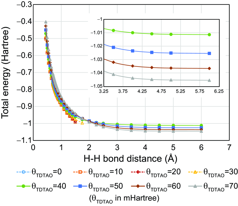
Figure 1: Potential energy surface of the first triplet excited state (1³$\Sigma_{u}^{+}$) computed using TDDFT ($\theta=0$ mHartree) and TDTAO-DFT with the PBE XC-functional, cc-pVDZ basis set and GEA version of $E_{\theta}$ functional Chai (2014) for TAO calculations. The inset shows a zoomed-in view for the large bond-distance regime.

The TDDFT results show imaginary frequencies beyond the H-H bond distance of $\sim 1.5$ Å. This is attributed to a poor ground-state reference, as mentioned previously, due to lack of incorporation of the non-dynamical correlation effects beyond this bond distance. In addition, this phenomenon is observed in TDTAO-DFT simulations for $\theta=0,10,20,$ and $30$ mHartree. However, for $\theta\geq 40$ mHartree, the imaginary-frequency issue is resolved.

We also note here that the requirement for a real-value $1^{3}\Sigma_{u}^{+}$ excitation energy mandates a higher threshold value for $\theta$ than that obtained through a self-consistent scheme Lin et al. (2017), which is around 15.5 mHartree. While a lower $\theta$ value is needed to describe the ground-state bond dissociation curves, our observation indicates that a higher $\theta$ value is needed for excitation properties and an optimal determination scheme for $\theta$ remains to be developed. One such direction is to include the excited state information in the post-SCF variational scheme similar to that outlined in Eq. 9 in Ref. 56.

Another advantageous aspect of TDTAO-DFT is that the energy of the first triplet excited (1³$\Sigma_{u}^{+}$) state in the dissociation limit correctly approaches the GS singlet energy. Fig. 2 shows the singlet-triplet (1¹$\Sigma_{g}^{+}$-1³$\Sigma_{u}^{+}$) vertical gap as a function of H-H bond dissociation computed using ground-state TAO-DFT, CCSD, and TDTAO-DFT. To compute the 1¹$\Sigma_{g}^{+}$-1³$\Sigma_{u}^{+}$ gap at the ground-state level (in order to mitigate the problem of imaginary frequencies in TDDFT), it was recommended to use the unrestricted ground-state SCF formalism for H₂ and other small molecules Cai and Reimers (2000); Proynov et al. (2010, 2012). However, this does not guarantee the convergence of the energy of the 1³$\Sigma_{u}^{+}$ state to that of the 1¹$\Sigma_{g}^{+}$ state at the bond dissociation limit for H₂ for TAO-DFT (Fig. 2).

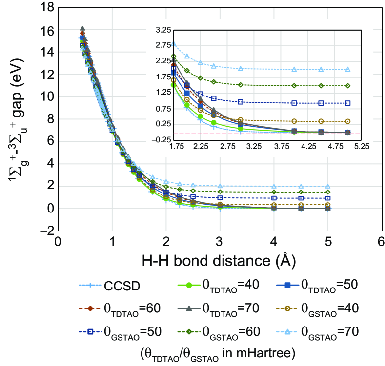
Figure 2: The energy gap as a function of H-H bond distance (in Å) between the singlet ground state (1¹$\Sigma_{g}^{+}$) and the first excited triplet state (1³$\Sigma_{u}^{+}$) calculated using TDTAO-DFT and unrestricted TAO-DFT with the PBE XC-functional and GEA $\theta$-functional. The equation-of-motion$-$coupled cluster singles doubles (EOM-CCSD) results are presented as a benchmark. The cc-pVDZ basis set was employed for all calculations. The inset shows a zoomed-in view for the large bond-distance regime.

This gap may violate the covalent nature of the ³$\Sigma_{u}^{+}$ state, where the energies of covalent states 1³$\Sigma_{u}^{+}$ and GS (1¹$\Sigma_{g}^{+}$) should be the same at the bond dissociation limit Gritsenko et al. (2000). In other words, at this limit, the electrons are located in the 1s orbitals of the corresponding atoms and are therefore, isolated enough with respect to one another. This gap increases with $\theta$ due to the increase in the energy of 1³$\Sigma_{u}^{+}$ and a simultaneous decrease in the energy of 1¹$\Sigma_{g}^{+}$ (this $\theta$-dependent decrease is also observed for the total energy of 1³$\Sigma_{u}^{+}$ calculated with TDTAO-DFT in Fig. 1). On the other hand, the trend obtained for TDTAO-DFT (Fig. 2) is in excellent agreement with that obtained using the equation-of-motion coupled-cluster singles and doubles (EOM-CCSD) method or observed in experiments Kouchi et al. (1997). EOM-CCSD is used here as a benchmark method since it is equivalent to FCI for a two-electron system like H2.

For the sake of completeness, we also computed the PESs of other excited states for H₂. The lowest six singlet and triplet excited states in TDTAO-DFT and TDDFT are demonstrated with low-lying PESs from EOM-CCSD in Figs. 3 (a) and (b).

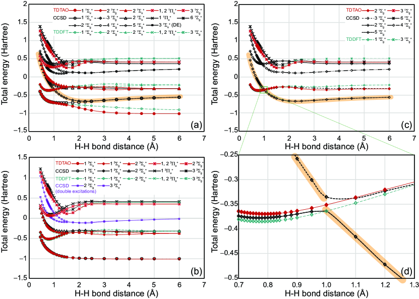
Figure 3: Potential energies of (a) singlet and (b) triplet excited states, computed using TDTAO-DFT (with $\theta$ = 40 mHartree and GEA $\theta$-functional), EOM-CCSD, and conventional TDDFT. (c) shows only the ¹$\Sigma_{g}^{+}$ states. (d) is a zoomed-in region showing the avoided crossing between two EOM-CCSD states that are not completely captured by either TDTAO-DFT or conventional TDDFT. The orange shaded regions in (a), (c), and (d) indicate portions of the EOM-CCSD curves that have double excitation character. DE in (a) signifies that, that CCSD state is double excitation in nature. PBE is selected as the XC-functional for all DFT calculations and cc-pVDZ as the basis set for all calculations.

The overall feature of singlet and triplet states from TDTAO-DFT is in excellent agreement with the EOM-CCSD results, except for the charge-transfer state (1¹$\Sigma_{u}^{+}$) and the missing states with double excitation character (purple curve with unfilled squares and golden yellow curves with unfilled diamonds in Figs. 3 (a) and (b)). We speculate that the problem with the 1¹$\Sigma_{u}^{+}$ state could be due to the usage of the simple adiabatic approximation to the $\text{xc}\theta$-kernel Casida et al. (2000); Runge and Gross (1984); Tozer (2003); Dreuw et al. (2003) as well as the time-independent occupation numbers in our formalism Giesbertz et al. (2008, 2009, 2010). The missing CCSD double excited states also indicate the inability of TDTAO-DFT to capture the avoided crossing between the first two ¹$\Sigma_{g}^{+}$ excited states (orange shaded regions as seen in Figs. 3 (a), (c), and (d)). A more detailed investigation is certainly required for resolving these challenges.

VI Relationship between $\theta$ and imaginary frequencies: A qualitative description

We perform a detailed analysis of the PESs with the different $\theta$ values to acquire more insight about the qualitative relationship between $\theta$ and the imaginary roots. Two molecular systems were chosen for this analysis, H2 and N2, and their S-T gaps are shown in Fig. 4. The problem of imaginary frequencies is fixed with TDTAO-DFT for a suitable choice of $\theta$, irrespective of the system under consideration, thereby indicating its versatility. However, we note that $\theta$ is a system-dependent quantity and a robust algorithm is needed to ascertain it. Based on the optimal choice of $\theta$, we observe that the S-T gap vanishes at the bond dissociation limit for N2 (Fig. 4(b)), similar to that in H2 (Fig. 4(a)). This is also in agreement with experiments Kadochnikov et al. (2013).

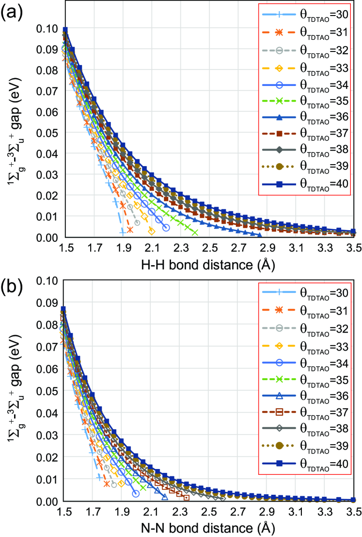
Figure 4: S-T gap of (a) H2 and (b) N2 with the bond distance and different $\theta$ (in mHartree) values, calculated using TDTAO-DFT with the PBE XC-functional, cc-pVDZ basis set and GEA version of $E_{\theta}$ functional Chai (2014). The filled symbols indicate potential energy surfaces without any imaginary frequencies.

VII Concluding Remarks

In summary, a time-dependent linear-response theory for predicting excited-state properties based on the TAO-DFT framework, TDTAO-DFT, is proposed. This theory takes advantage of TAO-DFT, where the spin-symmetry breaking problem of orbitals in ground-state SCF is resolved. As a result, TDTAO-DFT provides a correct description of low-lying triplet excited states, without imaginary energies, at the bond dissociation limit for a molecule. This was demonstrated through the dissociation curve of the hydrogen molecule, in which a reasonable lowest triplet state (1³$\Sigma_{u}^{+}$) is captured by TDTAO-DFT, but is not so, for TDDFT. Additionally, TAO-DFT (with a large fictitious temperature $\theta$) may produce an erratic gap between the 1³$\Sigma_{u}^{+}$ and ground states at the dissociation limit, which is resolved by TDTAO-DFT. The PESs for higher excited states of stretched H2 are also improved significantly as compared to TDDFT.

Supplementary Material

The Supplementary Material includes additional results and the numerical data presented in this work.

Data Availability Statement

The data that supports the findings of this study are available within the article and its supplementary material.

Appendix A A variational perspective of TAO-DFT

In this the section, we briefly present the derivation of the TAO-DFT KS-like equations based on an alternative, variational principle. The same variational approach is also employed in the derivation of the linear response theory, which will be presented in the latter section of this work.

According to the partition of energy functional Chai (2012, 2014), the functional derivative of the total energy functional can be expressed as

$$\frac{\delta E[\rho]}{\delta\phi_{i}(\mathbf{r})} = \frac{\delta T^{\textrm{TAO}}_{\mathrm{s}}}{\delta\phi_{i}(\mathbf{r})}+\frac{\delta V_{\textrm{ext}}}{\delta\phi_{i}(\mathbf{r})}+\frac{\delta E_{\textrm{Hxc}\theta}[\rho]}{\delta\phi_{i}(\mathbf{r})},$$ (26)

where $T^{\textrm{TAO}}_{\mathrm{s}}$ is the kinetic (free) energy functional, and $V_{\textrm{ext}}+E_{\textrm{Hxc}\theta}$ is the energy associated with the effective potential. The explicit derivative of the kinetic (free) energy functional would be

$$\frac{\delta T^{\textrm{TAO}}_{\mathrm{s}}}{\delta\phi^{*}_{j}(\mathbf{r^{\prime}})} = \frac{\delta}{\delta\phi^{*}_{j}(\mathbf{r^{\prime}})}\bigg{(}\sum_{i}f_{i}\int\mathrm{d}\mathbf{r}\,\phi^{*}_{i}(\mathbf{r})\,\hat{t}\,\phi_{i}(\mathbf{r})$$ (27)

$$+\theta\bigg{\{}\sum_{i}f_{i}\ln f_{i}+(1-f_{i})\ln(1-f_{i})\bigg{\}}\bigg{)}$$

$$= f_{j}\cdot\hat{t}\,\phi_{j}(\mathbf{r^{\prime}})+\sum_{i}\bigg{[}\frac{\delta f_{i}}{\delta\phi^{*}_{j}(\mathbf{r^{\prime}})}\cdot\int\mathrm{d}\mathbf{r}\,\phi^{*}_{i}(\mathbf{r})\,\hat{t}\,\phi_{i}(\mathbf{r})\bigg{]}$$

$$+\theta\sum_{i}\bigg{[}\big{\{}\ln f_{i}-\ln(1-f_{i})\big{\}}\cdot\frac{\delta f_{i}}{\delta\phi^{*}_{j}(\mathbf{r^{\prime}})}\bigg{]},$$

where $\hat{t}=-\nabla^{2}/2$ and $\delta\phi_{j}(\mathbf{r}^{\prime})/\delta\phi^{*}_{j}(\mathbf{r}^{\prime})=0$. Similarly, the derivatives of the energy term associated with external potential as well as the Hxc$\theta$ energy term are respectively,

$$\frac{\delta V_{\textrm{ext}}}{\delta\phi^{*}_{j}(\mathbf{r^{\prime}})} = \int\mathrm{d}\mathbf{r}^{\prime\prime}\frac{\delta\rho(r^{\prime\prime})}{\delta\phi^{*}_{j}(\mathbf{r^{\prime}})}\cdot\frac{\delta}{\delta\rho(r^{\prime\prime})}\bigg{[}\int\mathrm{d}\mathbf{r}\,v_{\textrm{ext}}(\mathbf{r})\rho(\mathbf{r})\bigg{]}$$

$$= \int\mathrm{d}\mathbf{r}\,v_{\textrm{ext}}(\mathbf{r})\frac{\delta\rho(\mathbf{r})}{\delta\phi^{*}_{j}(\mathbf{r^{\prime}})}$$

$$= f_{j}\cdot v_{\textrm{ext}}(\mathbf{r^{\prime}})\phi_{j}(\mathbf{r^{\prime}})$$

$$+\sum_{i}\bigg{(}\frac{\delta f_{i}}{\delta\phi^{*}_{j}(\mathbf{r^{\prime}})}\cdot\int\mathrm{d}\mathbf{r}\,v_{\textrm{ext}}(\mathbf{r})\phi^{*}_{i}(\mathbf{r})\phi_{i}(\mathbf{r})\bigg{)},$$

and

$$\frac{\delta E_{\textrm{Hxc}\theta}[\rho]}{\delta\phi^{*}_{j}(\mathbf{r^{\prime}})} = \int\mathrm{d}\mathbf{r}\,\frac{\delta\rho(\mathbf{r})}{\delta\phi^{*}_{j}(\mathbf{r^{\prime}})}\cdot\frac{\delta E_{\textrm{Hxc}\theta}[\rho]}{\delta\rho(\mathbf{r})}$$

$$= \int\mathrm{d}\mathbf{r}\,\frac{\delta\rho(\mathbf{r})}{\delta\phi^{*}_{j}(\mathbf{r^{\prime}})}\cdot v_{\textrm{Hxc}\theta}[\rho](\mathbf{r})$$

$$= f_{j}\cdot v_{\textrm{Hxc}\theta}(\mathbf{r^{\prime}})\phi_{j}(\mathbf{r^{\prime}})$$

$$+\sum_{i}\Big{[}\frac{\delta f_{i}}{\delta\phi^{*}_{j}(\mathbf{r^{\prime}})}\int\mathrm{d}\mathbf{r}v_{\textrm{Hxc}\theta}[\rho](\mathbf{r})\phi^{*}_{i}(\mathbf{r})\phi_{i}(\mathbf{r})\Big{]}.$$

Combining the three terms above, an explicit expression of the total energy functional is derived

$$\frac{\delta E[\rho]}{\delta\phi_{j}^{*}(\mathbf{r^{\prime}})} = \frac{\delta T^{\textrm{TAO}}_{\mathrm{s}}}{\delta\phi_{j}^{*}(\mathbf{r^{\prime}})}+\frac{\delta V_{\textrm{ext}}}{\delta\phi_{j}^{*}(\mathbf{r^{\prime}})}+\frac{\delta E_{\textrm{Hxc}\theta}[\rho]}{\delta\phi_{j}^{*}(\mathbf{r^{\prime}})}$$

$$= f_{j}\cdot\hat{t}\,\phi_{j}(\mathbf{r^{\prime}})+\sum_{i}\Big{[}\frac{\delta f_{i}}{\delta\phi^{*}_{j}(\mathbf{r^{\prime}})}\cdot\int\mathrm{d}\mathbf{r}\,\phi^{*}_{i}(\mathbf{r})\,\hat{t}\,\phi_{i}(\mathbf{r})\Big{]}$$

$$+\theta\sum_{i}\Big{[}\big{(}\ln f_{i}-\ln(1-f_{i})\big{)}\cdot\frac{\delta f_{i}}{\delta\phi^{*}_{j}(\mathbf{r^{\prime}})}\Big{]}$$

$$+f_{j}\cdot v_{\textrm{ext}}(\mathbf{r^{\prime}})\phi_{j}(\mathbf{r^{\prime}})$$

$$+\sum_{i}\Big{[}\frac{\delta f_{i}}{\delta\phi^{*}_{j}(\mathbf{r^{\prime}})}\cdot\int\mathrm{d}\mathbf{r}\,v_{\textrm{ext}}(\mathbf{r})\phi^{*}_{i}(\mathbf{r})\phi_{i}(\mathbf{r})\Big{]}$$

$$+f_{j}\cdot v_{\textrm{Hxc}\theta}(\mathbf{r^{\prime}})\phi_{j}(\mathbf{r^{\prime}})$$

$$+\sum_{i}\Big{[}\frac{\delta f_{i}}{\delta\phi^{*}_{j}(\mathbf{r^{\prime}})}\cdot\int\mathrm{d}\mathbf{r}\,v_{\textrm{Hxc}\theta}[\rho](\mathbf{r})\phi^{*}_{i}(\mathbf{r})\phi_{i}(\mathbf{r})\Big{]}$$

$$= f_{j}\cdot\big{[}\hat{t}+v_{\textrm{ext}}(\mathbf{r^{\prime}})+v_{\textrm{Hxc}\theta}[\rho](\mathbf{r^{\prime}})\big{]}\phi_{j}(\mathbf{r^{\prime}})$$

$$+\sum_{i}\frac{\delta f_{i}}{\delta\phi^{*}_{j}(\mathbf{r^{\prime}})}\cdot\bigg{\{}\theta\ln\bigg{(}\frac{f_{i}}{1-f_{i}}\bigg{)}$$

$$+\int\mathrm{d}\mathbf{r}\,\phi^{*}_{i}(\mathbf{r})\Big{[}\hat{t}+v_{\textrm{ext}}(\mathbf{r})+v_{\textrm{Hxc}\theta}[\rho](\mathbf{r})\Big{]}\phi_{i}(\mathbf{r})\bigg{\}}.$$

Enforcing the normalization conditions for both density and orbital functions, a Lagrangian is introduced

$$\mathcal{L}[\rho]=E[\rho] - \sum_{ij}\Big{[}\lambda_{ij}\int\mathrm{d}r\,\phi_{i}^{*}(\mathbf{r})\phi_{j}(\mathbf{r})-\delta_{ij}\Big{]}$$ (31)

$$- \mu\Big{[}\int\mathrm{d}\mathbf{r}\,\rho^{\mathrm{TAO}}(\mathbf{r})-N_{\mathrm{e}}\Big{]},$$

where $\{\lambda_{ij}\}$ and $\mu$ are Lagrange multipliers. Considering the functional derivative with respect to orbital functions

$$\frac{\delta\mathcal{L}[\rho]}{\delta\phi_{j}^{*}(\mathbf{r^{\prime}})} = f_{j}\cdot\big{[}\hat{t}+v_{\textrm{ext}}(\mathbf{r^{\prime}})+v_{\textrm{Hxc}\theta}[\rho](\mathbf{r^{\prime}})\big{]}\phi_{j}(\mathbf{r^{\prime}})$$ (32)

$$+\sum_{i}\frac{\delta f_{i}}{\delta\phi^{*}_{j}(\mathbf{r^{\prime}})}\cdot\Bigg{\{}\theta\ln\bigg{(}\frac{f_{i}}{1-f_{i}}\bigg{)}$$

$$+\int\mathrm{d}r\,\phi^{*}_{i}(\mathbf{r})\big{[}\hat{t}+v_{\textrm{ext}}(\mathbf{r})+v_{\textrm{Hxc}\theta}[\rho](\mathbf{r})\big{]}\phi_{i}(\mathbf{r})\Bigg{\}}$$

$$-\sum_{i}\lambda_{ji}\cdot\phi_{j}(\mathbf{r^{\prime}})-\mu\sum_{i}\frac{\delta f_{i}}{\delta\phi^{*}_{j}(\mathbf{r^{\prime}})}-\mu f_{j}\cdot\phi_{j}(\mathbf{r^{\prime}})$$

$$= f_{j}\cdot\big{[}\hat{t}+v_{\textrm{ext}}(\mathbf{r^{\prime}})+v_{\textrm{Hxc}\theta}[\rho](\mathbf{r^{\prime}})\big{]}\phi_{j}(\mathbf{r^{\prime}})$$

$$+\sum_{i}\bigg{\{}\varepsilon_{i}-\theta\big{[}\frac{1}{\theta}(\varepsilon_{i}-\mu)\big{]}\bigg{\}}\cdot\frac{\delta f_{i}}{\delta\phi^{*}_{j}(\mathbf{r^{\prime}})}$$

$$-\sum_{i}\lambda_{ji}\cdot\phi_{i}(\mathbf{r^{\prime}})-\mu\sum_{i}\frac{\delta f_{i}}{\delta\phi^{*}_{j}(\mathbf{r^{\prime}})}-\mu f_{j}\cdot\phi_{j}(\mathbf{r^{\prime}})$$

$$= f_{j}\cdot\big{[}\hat{t}+v_{\textrm{ext}}(\mathbf{r^{\prime}})+v_{\textrm{Hxc}\theta}[\rho](\mathbf{r^{\prime}})\big{]}\phi_{j}(\mathbf{r^{\prime}})$$

$$+\mu\sum_{i}\frac{\delta f_{i}}{\delta\phi^{*}_{j}(\mathbf{r^{\prime}})}-\sum_{i}\lambda_{ji}\cdot\phi_{i}(\mathbf{r^{\prime}})$$

$$-\mu\sum_{i}\frac{\delta f_{i}}{\delta\phi^{*}_{j}(\mathbf{r^{\prime}})}-\mu f_{j}\cdot\phi_{j}(\mathbf{r^{\prime}})$$

$$= f_{j}\cdot\big{[}\hat{t}+v_{\textrm{ext}}(\mathbf{r^{\prime}})+v_{\textrm{Hxc}\theta}[\rho](\mathbf{r^{\prime}})\big{]}\phi_{j}(\mathbf{r^{\prime}})$$

$$-\Big{(}\lambda_{jj}+\mu f_{j}\Big{)}\cdot\phi_{j}(\mathbf{r^{\prime}})+\sum^{i\neq j}_{i}\lambda_{ji}\cdot\phi_{i}(\mathbf{r^{\prime}}).$$

and using the variational condition $\delta\mathcal{L}[\rho]/\delta\phi_{j}^{*}(\mathbf{r^{\prime}})=0$, one obtains

$$\big{[}\hat{t}+v_{\textrm{ext}}(\mathbf{r^{\prime}})+v_{\textrm{Hxc}\theta}[\rho](\mathbf{r^{\prime}})\big{]}\phi_{j}(\mathbf{r^{\prime}})$$

$$\,\,\,=(f_{j}^{-1}\lambda_{jj}+\mu)\cdot\phi_{j}(\mathbf{r^{\prime}})+f_{j}^{-1}\sum_{i}^{i\neq j}\lambda_{ji}\cdot\phi_{i}(\mathbf{r^{\prime}}).$$ (33)

Note that the second term in Eq. 32 indicates that it is necessary to introduce the entropy term $\theta[\sum_{i}f_{i}\ln f_{i}+(1-f_{i})\ln(1-f_{i})]$ to the kinetic functional, in order to preserve the correct variational property such that the derivative terms arising from $v_{\text{ext}}$ and $v_{\text{Hxc}\theta}$ (last terms in Eqs. LABEL:vext_tao and LABEL:vhxctheta) are compensated.

With canonical orbital assumption (because the orbitals are orthonormal to one another), the equation can be recast into an eigenvalue equation, similar to a KS-like equation

$$\hat{h}^{\textrm{TAO}}[\rho](\mathbf{r})\phi_{i}(\mathbf{r})=\varepsilon_{i}\cdot\phi_{i}(\mathbf{r}),$$ (34)

where $\hat{h}^{\textrm{TAO}}=\hat{t}+v_{\textrm{ext}}+v_{\textrm{Hxc}\theta}$ and $\varepsilon_{i}=f_{i}^{-1}\lambda_{ii}+\mu$.

Appendix B Detailed derivation of LR-TDTAO-DFT

B.1 Variational principle for TAO action functional and TD effective potential

Starting from the action variational principle Gross and Kohn (1990) and its modified form Vignale (2008), we have the general definitions of action functionals for a physical system,

$$A[\rho]=\int^{\tau}_{0}\mathrm{d}t\,\Big{\langle}\Psi(t)\Big{|}\bigg{(}\frac{\partial}{\partial t}-\hat{H}\bigg{)}\Big{|}\Psi(t)\Big{\rangle},$$ (35)

$$B[\rho]=A[\rho]+\int\mathrm{d}t\int\mathrm{d}\mathbf{r}\,v_{\mathrm{ext}}(\mathbf{r},t)\rho(\mathbf{r},t),$$ (36)

$$\frac{\delta B[\rho]}{\delta\rho(\mathbf{r},t)}=v_{\mathrm{ext}}(\mathbf{r},t)+i\Bigg{\langle}\Psi[\rho](\tau)\Bigg{|}\frac{\delta\Psi_{[}\rho;\tau]}{\delta\rho(\mathbf{r},t)}\Bigg{\rangle},$$ (37)

where $\Psi[\rho;\tau]$ represents the wavefunction at time $t$ and $\tau$ denotes the upper bound of time-integral.

For a TDTAO system, the definition of universal action functionals can be written similarly, following that of the conventional TDDFT scheme Vignale (2008),

$$\frac{\delta A_{\textrm{TAO}}[\rho]}{\delta\rho(\mathbf{r},t)}=i\Bigg{\langle}\Psi_{\mathrm{TAO}}[\rho](\tau)\Bigg{|}\frac{\delta\Psi_{\mathrm{TAO}}[\rho;\tau]}{\delta\rho(\mathbf{r},t)}\Bigg{\rangle}$$ (38)

$$B_{\textrm{TAO}}[\rho]=A_{\textrm{TAO}}[\rho]+\int^{\tau}_{0}\mathrm{d}t\mathrm{d}\mathbf{r}\,v_{\mathrm{eff}}(\mathbf{r},t)\rho(\mathbf{r},t).$$ (39)

The TD effective potential for TAO can be expressed as

$$v_{\mathrm{eff}}(\mathbf{r},t)=\frac{\delta B_{\textrm{TAO}}[\rho]}{\delta\rho(\mathbf{r},t)}+i\Bigg{\langle}\Psi_{\mathrm{TAO}}[\rho](\tau)\Bigg{|}\frac{\delta\Psi_{\mathrm{TAO}}[\rho;\tau]}{\delta\rho(\mathbf{r},t)}\Bigg{\rangle}.$$

One can define the difference between the two functionals as

$$A_{\textrm{Hxc}\theta}[\rho]=B_{\textrm{TAO}}[\rho]-B[\rho],$$ (41)

which is the TAO extension of Hartree-exchange-correlation functionals. Summarizing the equations above, similar to TDDFT, one can recast the effective potential in TAO as

$$v_{\mathrm{Hxc}\theta}(\mathbf{r},t) = \frac{\delta A_{\textrm{Hxc}\theta}[\rho]}{\delta\rho(\mathbf{r},t)}$$ (42)

$$= v_{\textrm{eff}}(\mathbf{r},t)+i\Bigg{\langle}\Psi_{\mathrm{TAO}}[\rho](\tau)\Bigg{|}\frac{\delta\Psi_{\mathrm{TAO}}[\rho;\tau]}{\delta\rho(\mathbf{r},t)}\Bigg{\rangle}$$

$$-v_{\mathrm{ext}}(\mathbf{r},t)-i\Bigg{\langle}\Psi[\rho](\tau)\Bigg{|}\frac{\delta\Psi[\rho;\tau]}{\delta\rho(\mathbf{r},t)}\Bigg{\rangle}.$$

B.2 Density-density response function

Here we show that the linear response equation can also be constructed inversely,

$$\delta\rho(\mathbf{r}\,t)=\int\textrm{d}\mathbf{r^{\prime}}\textrm{d}t^{\prime}\,\chi_{\textrm{s}}^{\mathrm{TAO}}(\mathbf{r}\,t,\mathbf{r}^{\prime}\,t^{\prime})\,\delta v^{\textrm{TAO}}_{\textrm{eff}}(\mathbf{r}^{\prime}\,t^{\prime}),$$ (43)

where

$$\chi_{\textrm{s}}^{\mathrm{TAO}}(\mathbf{r}\,t,\mathbf{r}^{\prime}\,t^{\prime})\equiv\frac{\delta\rho^{\mathrm{TAO}}(\mathbf{r},t)}{\delta v^{{\mathrm{TAO}}}_{\mathrm{eff}}(\mathbf{r}^{\prime},t^{\prime})}$$ (44)

is the density-density response function for a non-interacting TAO system. With the density expression in terms of TD orbitals, one obtains

$$\chi_{\textrm{s}}^{\mathrm{TAO}}(\mathbf{r}\,t,\mathbf{r}^{\prime}\,t^{\prime}) = \frac{\delta\rho^{\mathrm{TAO}}(\mathbf{r},t)}{\delta v^{{\mathrm{TAO}}}_{\mathrm{eff}}(\mathbf{r}^{\prime},t^{\prime})}=\frac{\delta\Big{[}\sum_{p}f_{p}\,\phi^{*}_{p}(\mathbf{r},t)\phi_{p}(\mathbf{r},t)\Big{]}}{\delta v^{{\mathrm{TAO}}}_{\mathrm{eff}}(\mathbf{r}^{\prime},t^{\prime})}$$ (45)

$$= \sum_{p}f_{p}\frac{\delta\Big{[}\phi^{*}_{p}(\mathbf{r},t)\phi_{p}(\mathbf{r},t)\Big{]}}{\delta v^{{\mathrm{TAO}}}_{\mathrm{eff}}(\mathbf{r}^{\prime},t^{\prime})}$$

$$= \sum_{p}f_{p}\bigg{[}\frac{\delta\phi^{*}_{p}(\mathbf{r},t)}{\delta v^{{\mathrm{TAO}}}_{\mathrm{eff}}(\mathbf{r}^{\prime},t^{\prime})}\phi^{\circ}_{p}(\mathbf{r},t)$$

$$\,\,\,\,\,\,\,\,\,\,\,\,\,\,\,\,\,\,\,\,\,+\,\phi^{\circ*}_{p}(\mathbf{r},t)\frac{\delta\phi_{p}(\mathbf{r},t)}{\delta v^{{\mathrm{TAO}}}_{\mathrm{eff}}(\mathbf{r}^{\prime},t^{\prime})}\bigg{]},$$

where $\phi^{\circ}_{p}(\mathbf{r},t)$ and its complex conjugate represent the evolution of the TD orbitals in the absence of any TD perturbation (i.e., the TD external field). Applying the first-order perturbation theory, the TD orbital functions in a TD external field can be described by the following equation

$$\phi_{p}(\mathbf{r},t) = \bigg{[}1-i\int^{t}_{0}\mathrm{d}t^{\prime}\sum_{rs}^{r\neq p}\phi^{\circ}_{r}(\mathbf{r})\,e^{-i\varepsilon_{r}(t-t^{\prime})}$$

$$\,\,\,\,\,\,\times\Big{[}\int\mathrm{d}\mathbf{r}^{\prime}\,\phi^{\circ*}_{r}(\mathbf{r}^{\prime})\delta v^{{\mathrm{TAO}}}_{\mathrm{eff}}(\mathbf{r}^{\prime},t^{\prime})\phi^{\circ}_{s}(\mathbf{r}^{\prime})\Big{]}e^{-i\varepsilon_{s}t^{\prime}}$$

$$\,\,\,\,\,\,\times\int\mathrm{d}\mathbf{r}\,\phi^{\circ*}_{s}(\mathbf{r})\bigg{]}\phi^{\circ}_{p}(\mathbf{r})$$

$$= \phi^{\circ}_{p}(\mathbf{r})-i\,e^{-i\varepsilon_{r}t}\int^{t}_{0}\mathrm{d}t^{\prime}\sum_{r,\,r\neq p}\phi^{\circ}_{r}(\mathbf{r})$$

$$\,\,\,\,\,\,\times\Big{[}\int\mathrm{d}\mathbf{r}^{\prime}\,\phi^{\circ*}_{r}(\mathbf{r}^{\prime})\delta v^{{\mathrm{TAO}}}_{\mathrm{eff}}(\mathbf{r}^{\prime},t^{\prime})\phi^{\circ}_{p}(\mathbf{r}^{\prime})\Big{]}e^{-i(\varepsilon_{p}-\varepsilon_{r})t^{\prime}},$$

and the corresponding orbital response functions are expressed explicitly in terms of initial orbitals (ground-state TAO orbitals) and orbital energies

$$\frac{\delta\phi_{p}(\mathbf{r},t)}{\delta v^{{\mathrm{TAO}}}_{\mathrm{eff}}(\mathbf{r}^{\prime},t^{\prime})} = -i\Theta(t-t^{\prime})e^{-i\varepsilon_{r}t}$$

$$\,\,\,\,\,\,\times\sum_{r,\,r\neq p}\phi^{\circ}_{r}(\mathbf{r})\phi^{\circ*}_{r}(\mathbf{r}^{\prime})\phi^{\circ}_{p}(\mathbf{r}^{\prime})e^{-i(\varepsilon_{p}-\varepsilon_{r})t^{\prime}}$$

$$\frac{\delta\phi^{*}_{p}(\mathbf{r},t)}{\delta v^{{\mathrm{TAO}}}_{\mathrm{eff}}(\mathbf{r}^{\prime},t^{\prime})} = i\Theta(t-t^{\prime})e^{i\varepsilon_{r}t}$$

$$\,\,\,\,\,\,\times\sum_{r,\,r\neq p}\phi^{\circ*}_{r}(\mathbf{r})\phi^{\circ}_{r}(\mathbf{r}^{\prime})\phi^{\circ*}_{p}(\mathbf{r}^{\prime})e^{i(\varepsilon_{p}-\varepsilon_{r})t^{\prime}}.$$

Combining Eq. 45 and Eq. LABEL:orbital_response_function, the time-domain non-interacting response function in TDTAO-DFT can be evaluated as follows

$$\chi_{\textrm{s}}^{\mathrm{TAO}}(\mathbf{r}\,t,\mathbf{r}^{\prime}\,t^{\prime}) = \sum_{p}f_{p}\Bigg{\{}\bigg{[}i\Theta(t-t^{\prime})\,e^{i\varepsilon_{r}t}\sum_{r,\,r\neq p}\phi^{\circ*}_{r}(\mathbf{r})\phi^{\circ}_{r}(\mathbf{r}^{\prime})\phi^{\circ*}_{p}(\mathbf{r}^{\prime})e^{i(\varepsilon_{p}-\varepsilon_{r})t^{\prime}}\bigg{]}\phi^{\circ}_{p}(\mathbf{r},t)$$

$$\,\,\,\,\,\,\,\,\,\,\,\,\,\,\,\,\,\,\,\,+\,\phi^{\circ*}_{p}(\mathbf{r},t)\bigg{[}-i\Theta(t-t^{\prime})\,e^{-i\varepsilon_{r}t}\sum_{r,\,r\neq p}\phi^{\circ}_{r}(\mathbf{r})\phi^{\circ*}_{r}(\mathbf{r}^{\prime})\phi^{\circ}_{p}(\mathbf{r}^{\prime})e^{-i(\varepsilon_{p}-\varepsilon_{r})t^{\prime}}\bigg{]}\Bigg{\}}$$

$$= i\sum_{pr}^{r\neq p}f_{p}\Theta(t-t^{\prime})\Bigg{\{}\phi^{\circ}_{p}(\mathbf{r})\phi^{\circ*}_{r}(\mathbf{r})\phi^{\circ}_{r}(\mathbf{r}^{\prime})\phi^{\circ*}_{p}(\mathbf{r}^{\prime})e^{i(\varepsilon_{r}-\varepsilon_{p})(t-t^{\prime})}-\phi^{\circ*}_{p}(\mathbf{r})\phi^{\circ}_{r}(\mathbf{r})\phi^{\circ*}_{r}(\mathbf{r}^{\prime})\phi^{\circ}_{p}(\mathbf{r}^{\prime})e^{-i(\varepsilon_{r}-\varepsilon_{p})(t-t^{\prime})}\Bigg{\}}$$

Performing a Fourier transformation, the corresponding frequency-domain expression becomes

$$\chi_{\textrm{s}}^{\mathrm{TAO}}(\mathbf{r},\mathbf{r}^{\prime},\omega) = \sum_{pr}^{r\neq p}f_{p}\Bigg{\{}\frac{\phi^{\circ}_{p}(\mathbf{r})\phi^{\circ*}_{r}(\mathbf{r})\phi^{\circ}_{r}(\mathbf{r}^{\prime})\phi^{\circ*}_{p}(\mathbf{r}^{\prime})}{\omega-(\varepsilon_{r}-\varepsilon_{p})+i\eta}$$ (49)

$$\,\,\,\,\,\,-\frac{\phi^{\circ*}_{p}(\mathbf{r})\phi^{\circ}_{r}(\mathbf{r})\phi^{\circ*}_{r}(\mathbf{r}^{\prime})\phi^{\circ}_{p}(\mathbf{r}^{\prime})}{\omega+(\varepsilon_{r}-\varepsilon_{p})+i\eta}\Bigg{\}}$$

$$= \sum_{pr}^{r\neq p}(f_{p}-f_{r})\frac{\phi^{\circ*}_{p}(\mathbf{r}^{\prime})\phi^{\circ}_{r}(\mathbf{r}^{\prime})\phi^{\circ*}_{r}(\mathbf{r})\phi^{\circ}_{p}(\mathbf{r})}{\omega-(\varepsilon_{r}-\varepsilon_{p})+i\eta},$$

$$\text{ where}\,\eta\rightarrow 0.$$

We note that there are no self-transition terms in both Eq. 49 and Eq. LABEL:orbital_PT, since every TD orbital is considered as an orthonormalized function at any given instant of time. As a result, an explicit response function for a non-interacting reference system (TAO system) is obtained, and the resulting expression is similar to the conventional TDDFT Petersilka et al. (1996).

B.3 Alternative path to the Casida’s equation

Recall the partition of effective potential Ullrich (2012)

$$\delta v_{\textrm{eff}}^{\textrm{TAO}}(\mathbf{r},\omega) = \delta v_{\textrm{ext}}(\mathbf{r},\omega)+\int\mathrm{d}\mathbf{r}_{1}\,\delta\rho(\mathbf{r}_{1},\omega)\cdot\mathbbm{f}_{\textrm{Hxc}\theta}(\mathbf{r},\mathbf{r}_{1},\omega)$$ (50)

$$= \delta v_{\textrm{ext}}(\mathbf{r},\omega)+\delta v_{\textrm{Hxc}\theta}[\rho](\mathbf{r},\omega).$$

where $\mathbbm{f}_{\textrm{Hxc}\theta}$ is the Fock matrix defined in Eq. 17 in the main manuscript. Since an infinitesimal external field change is considered ($\delta v_{\textrm{ext}}(\mathbf{r}_{1},\omega)\rightarrow 0$) Dreuw and Head-Gordon (2005); Casida (1995), Eq. 43 can be recast into

$$\delta\rho(\mathbf{r},\omega) = \int\mathrm{d}\mathbf{r}_{1}\int\mathrm{d}\mathbf{r}_{2}\,\chi_{\textrm{s}}^{\textrm{TAO}}(\mathbf{r},\mathbf{r}_{1},\omega)$$ (51)

$$\times\delta\rho(\mathbf{r}_{2},\omega)\cdot\mathbbm{f}_{\textrm{Hxc}\theta}(\mathbf{r}_{1},\mathbf{r}_{2},\omega).$$

If $\int\mathrm{d}\mathbf{r}\,\mathbbm{f}_{\textrm{Hxc}\theta}(\mathbf{r}^{\prime},\mathbf{r},\omega)$ is operated on both sides of the equation, one obtains an iterative formula

$$\delta v_{\textrm{Hxc}\theta}(\mathbf{r},\omega) = \int\mathrm{d}\mathbf{r}_{1}\int\mathrm{d}\mathbf{r}_{2}\mathbbm{f}_{\textrm{Hxc}\theta}(\mathbf{r},\mathbf{r}_{1},\omega)$$ (52)

$$\times\chi_{\textrm{s}}^{\textrm{TAO}}(\mathbf{r}_{1},\mathbf{r}_{2},\omega)\delta v_{\textrm{Hxc}\theta}(\mathbf{r}_{2},\omega)$$

Recalling the explicit expression of non-interacting response function in Eq. 49, Eq. 52 can be reformulated into

$$\delta v^{\textrm{Hxc}\theta}_{rs}(\omega) = \sum_{pq}^{q\neq p}\int\mathrm{d}\mathbf{r}\int\mathrm{d}\mathbf{r}_{1}\,\phi^{\circ*}_{r}(\mathbf{r})\phi^{\circ}_{s}(\mathbf{r})\phi^{\circ*}_{q}(\mathbf{r}_{1})\phi^{\circ}_{p}(\mathbf{r}_{1})$$

$$\,\,\,\,\,\,\times\,\mathbbm{f}_{\textrm{Hxc}\theta}(\mathbf{r},\mathbf{r}_{1},\omega)\bigg{[}\frac{(f_{p}-f_{q})\cdot\delta v^{\textrm{Hxc}\theta}_{pq}(\omega)}{\omega-(\varepsilon_{q}-\varepsilon_{p})+i\eta}\bigg{]},$$

where $\delta v^{\textrm{Hxc}\theta}_{rs}(\omega)=\int\mathrm{d}\mathbf{r}\,\phi^{\circ*}_{r}(\mathbf{r})\phi^{\circ}_{s}(\mathbf{r})\delta v_{\textrm{Hxc}\theta}(\mathbf{r},\omega)$ is the Hxc$\theta$ potential projected on the single-particle basis set. Similar to the derivation in main manuscript, the two-electron integral is defined as follows:

$$\big{(}rs\big{|}\mathbbm{f}_{\textrm{Hxc}\theta}(\omega)\big{|}pq\big{)}$$ (54)

$$\equiv\int\mathrm{d}\mathbf{r}\,\phi^{\circ*}_{r}(\mathbf{r})\phi^{\circ}_{s}(\mathbf{r})\int\mathrm{d}\mathbf{r}_{1}\,\phi^{\circ*}_{q}(\mathbf{r}_{1})\phi^{\circ}_{p}(\mathbf{r}_{1})\mathbbm{f}_{\textrm{Hxc}\theta}(\mathbf{r},\mathbf{r}_{1},\omega).$$

With a rescaling factor $[\omega-(\varepsilon_{s}-\varepsilon_{r})+i\eta]$, an iterative equation in a finite basis set is obtained

$$\Big{[}\omega-(\varepsilon_{s}-\varepsilon_{r})\Big{]}\cdot\Omega^{\mathrm{L}}_{rs}(\omega)$$

$$=\sum_{pq}^{q\neq p}\bigg{[}\big{(}rs\big{|}\mathbbm{f}_{\textrm{Hxc}\theta}(\omega)\big{|}pq\big{)}(f_{p}-f_{q})\bigg{]}\cdot\Omega^{\mathrm{L}}_{pq}(\omega),$$ (55)

where

$$\Omega^{\mathrm{L}}_{rs}(\omega)\equiv\frac{\delta v^{\textrm{Hxc}\theta}_{rs}(\omega)}{\omega-(\varepsilon_{s}-\varepsilon_{r})+i\eta}.$$ (56)

Within ALDA, the corresponding eigenvalue equation would be

$$\sum_{pq}\bigg{[}(\varepsilon_{q}-\varepsilon_{p})\delta_{qs}\delta_{pr}-\big{(}rs\big{|}\mathbbm{f}_{\textrm{Hxc}\theta}\big{|}pq\big{)}(f_{q}-f_{p})\bigg{]}\Omega^{\mathrm{L}}_{k,pq}$$

$$\,\,\,\,=\omega_{k}\cdot\Omega^{\mathrm{L}}_{k,rs},$$ (57)

where $k$ denotes the $k$-th eigenvalue. We note that this eigenvalue equation is not exactly the same as Eq. 19 the main text. However, because of the transpose relation between the two matrices, they will generate the same eigenspectra.

Appendix C Relaxed idempotency condition

In conventional TDDFT, transitions between orbital are pre-selected by the idempotency condition Dreuw and Head-Gordon (2005), which is derived from a single-determinant assumption, and can be formulated as

$$(f_{p}+f_{q}-1)\delta P_{pq}=0,$$ (58)

where $P_{pq}$ is a matrix element of transition density matrices. This condition leads to the result that only transitions between occupied and virtual orbitals would contribute to a physical (single) excitation. On the other hand, since the single-determinant assumption is removed from TAO-DFT, we consider an alternative invariant assumption based on the recurrence relation of the derivative of Fermi function

$$\frac{\partial f_{p}}{\partial\varepsilon_{p}}=-(f_{p}-f_{p}^{2})/\theta,$$ (59)

or in matrix representation is

$$\frac{\partial\mathbf{P}_{0}}{\partial\mathbf{F}_{0}}=-(\mathbf{P}_{0}-\mathbf{P}_{0}^{2})/\theta,$$ (60)

where $\mathbf{P}_{0}-\mathbf{P}_{0}^{2}$ on the left-hand-side implies a relaxed idempotency feature of TAO one-particle density matrix. In other words, instead of equating to zero, $\mathbf{P}_{0}-\mathbf{P}_{0}^{2}$ is associated with another constant, $\theta\cdot{\partial\mathbf{P}_{0}}/{\partial\mathbf{F}_{0}}$. To employ the relaxed condition in excited state TAO, we further assume that the simple partial derivative form would be preserved in the TD extension of ${\partial\mathbf{P}_{0}}/{\partial\mathbf{F}_{0}}$. Recall the total functional derivative of the density matrix

$$\delta(\mathbf{P}-\mathbf{P}^{2})=\delta\mathbf{P}-\mathbf{P}_{0}\cdot\delta\mathbf{P}-\delta\mathbf{P}\cdot\mathbf{P}_{0},$$ (61)

and combine it with Eq. 59

$$\delta P_{pq}-f_{p}\cdot\delta P_{pq}-\delta P_{pq}\cdot f_{q} = -(f_{p}+f_{q}-1)\delta P_{pq}$$ (62)

$$= -\theta\cdot\delta\bigg{[}\frac{\partial\mathbf{P}}{\partial\mathbf{F}}\bigg{]}_{pq},$$

where $\delta[{\partial\mathbf{P}}/{\partial\mathbf{F}}]_{pq}$ is not a explicit derivative and is assumed as an infinitesimal constant. Therefore, the relaxed condition is proposed as follows:

$$(f_{p}+f_{q}-1)\delta P_{pq}\propto\theta.$$ (63)

Note that the original idempotency condition would be preserved when the KS limit is considered ($\theta\rightarrow 0$). Based on the relaxed condition, an excitation should be dominated by those $p$ and $q$ terms with $(f_{p}+f_{q})$ tending to 1. Therefore, to reduce the interference from spurious excitations Giesbertz et al. (2010), only transitions between strongly occupied orbitals and strongly virtual orbitals, where $(f_{p}+f_{q}-1)$ is minimized, are considered in the current version of TDTAO-DFT. The criteria to classify orbitals are

$$f_{p\in\text{occ.}}\geq\frac{1}{2} \varepsilon_{p\in\text{occ.}}\leq\mu,$$ or

$$f_{q\in\text{vir.}}\leq\frac{1}{2} \varepsilon_{q\in\text{vir.}}\geq\mu.$$ or (64)

References

• Hohenberg and Kohn (1964) P. Hohenberg and W. Kohn, Phys. Rev. 136, B864 (1964).
• Kohn and Sham (1965) W. Kohn and L. J. Sham, Phys. Rev. 140, A1133 (1965).
• Jones (2015) R. O. Jones, Rev. Mod. Phys. 87, 897 (2015).
• Becke (2014) A. D. Becke, J. Chem. Phys. 140, 18A301 (2014).
• Mardirossian and Head-Gordon (2017) N. Mardirossian and M. Head-Gordon, Mol. Phys. 115, 2315 (2017).
• Runge and Gross (1984) E. Runge and E. K. U. Gross, Phys. Rev. Lett. 52, 997 (1984).
• Petersilka et al. (1996) M. Petersilka, U. J. Gossmann,  and E. K. U. Gross, Phys. Rev. Lett. 76, 1212 (1996).
• Casida (1995) M. E. Casida, “Time-Dependent Density Functional Response Theory for Molecules $|$ Recent Advances in Density Functional Methods,”  (WORLD SCIENTIFIC, 1995) pp. 155–192.
• Dreuw and Head-Gordon (2005) A. Dreuw and M. Head-Gordon, Chem. Rev. 105, 4009 (2005).
• Deskevich et al. (2006) M. P. Deskevich, M. Y. Hayes, K. Takahashi, R. T. Skodje,  and D. J. Nesbitt, J. Chem. Phys. 124, 224303 (2006).
• Tavernelli et al. (2005) I. Tavernelli, U. F. Röhrig,  and U. Rothlisberger, Mol. Phys. 103, 963 (2005).
• Toivonen et al. (2006) T. L. J. Toivonen, T. I. Hukka, O. Cramariuc, T. T. Rantala,  and H. Lemmetyinen, J. Phys. Chem. A 110, 12213 (2006).
• Hirata and Head-Gordon (1999) S. Hirata and M. Head-Gordon, Chem. Phys. Lett. 314, 291 (1999).
• Stratmann et al. (1998) R. E. Stratmann, G. E. Scuseria,  and M. J. Frisch, J. Chem. Phys. 109, 8218 (1998).
• Hsu et al. (2001) C.-P. Hsu, S. Hirata,  and M. Head-Gordon, J. Phys. Chem. A 105, 451 (2001).
• Levine et al. (2006) B. G. Levine, C. Ko, J. Quenneville,  and T. J. Martínez, Mol. Phys. 104, 1039 (2006).
• Filatov (2013) M. Filatov, J. Chem. Theory Comput. 9, 4526 (2013).
• Gritsenko et al. (2000) O. V. Gritsenko, S. J. A. van Gisbergen, A. Görling,  and E. J. Baerends, J. Chem. Phys. 113, 8478 (2000).
• Casida et al. (2000) M. E. Casida, F. Gutierrez, J. Guan, F.-X. Gadea, D. Salahub,  and J.-P. Daudey, J. Chem. Phys. 113, 7062 (2000).
• Becke (2005) A. D. Becke, J. Chem. Phys. 122, 064101 (2005).
• Becke (2013) A. D. Becke, J. Chem. Phys. 138, 074109 (2013).
• Proynov et al. (2010) E. Proynov, Y. Shao,  and J. Kong, Chem. Phys. Lett. 493, 381 (2010).
• Proynov et al. (2012) E. Proynov, F. Liu, Y. Shao,  and J. Kong, J. Chem. Phys. 136, 034102 (2012).
• Kong and Proynov (2016) J. Kong and E. Proynov, J. Chem. Theory Comput. 12, 133 (2016).
• Gräfenstein and Cremer (2000) J. Gräfenstein and D. Cremer, Chem. Phys. Lett. 316, 569 (2000).
• Li Manni et al. (2014) G. Li Manni, R. K. Carlson, S. Luo, D. Ma, J. Olsen, D. G. Truhlar,  and L. Gagliardi, J. Chem. Theory Comput. 10, 3669 (2014).
• Li Manni et al. (2016) G. Li Manni, R. K. Carlson, S. Luo, D. Ma, J. Olsen, D. G. Truhlar,  and L. Gagliardi, J. Chem. Theory Comput. 12, 458 (2016).
• Fromager et al. (2013) E. Fromager, S. Knecht,  and H. J. A. Jensen, J. Chem. Phys. 138, 084101 (2013).
• Sharkas et al. (2012) K. Sharkas, A. Savin, H. J. A. Jensen,  and J. Toulouse, J. Chem. Phys. 137, 044104 (2012).
• Stanton and Gauss (1994) J. F. Stanton and J. Gauss, J. Chem. Phys. 101, 8938 (1994).
• Nooijen and Bartlett (1998) M. Nooijen and R. J. Bartlett, J. Chem. Phys. 102, 3629 (1998).
• Shao et al. (2003) Y. Shao, M. Head-Gordon,  and A. I. Krylov, J. Chem. Phys. 118, 4807 (2003).
• Chai (2012) J.-D. Chai, J. Chem. Phys. 136, 154104 (2012).
• Chai (2014) J.-D. Chai, J. Chem. Phys. 140, 18A521 (2014).
• Chai (2017) J.-D. Chai, J. Chem. Phys. 146, 044102 (2017).
• Xuan et al. (2019) F. Xuan, J.-D. Chai,  and H. Su, ACS Omega 4, 7675 (2019).
• Lin et al. (2017) C.-Y. Lin, K. Hui, J.-H. Chung,  and J.-D. Chai, RSC Adv. 7, 50496 (2017).
• Wu and Chai (2015) C.-S. Wu and J.-D. Chai, J. Chem. Theory Comput. 11, 2003 (2015).
• Yeh and Chai (2016) C.-N. Yeh and J.-D. Chai, Sci. Rep. 6, 30562 (2016).
• Seenithurai and Chai (2016) S. Seenithurai and J.-D. Chai, Sci. Rep. 6, 33081 (2016).
• Wu et al. (2016) C.-S. Wu, P.-Y. Lee,  and J.-D. Chai, Sci. Rep. 6, 37249 (2016).
• Seenithurai and Chai (2017) S. Seenithurai and J.-D. Chai, Sci. Rep. 7, 4966 (2017).
• Seenithurai and Chai (2018) S. Seenithurai and J.-D. Chai, Sci. Rep. 8, 13538 (2018).
• Yeh et al. (2018) C.-N. Yeh, C. Wu, H. Su,  and J.-D. Chai, RSC Adv. 8, 34350 (2018).
• Chung and Chai (2019) J.-H. Chung and J.-D. Chai, Sci. Rep. 9, 2907 (2019).
• Yang et al. (2016) Y. Yang, E. R. Davidson,  and W. Yang, Proc. Natl Acad. Sci. 113, E5098 (2016).
• Hachmann et al. (2007) J. Hachmann, J. J. Dorando, M. Aviles,  and G. K.-L. Chan, J. Chem. Phys. 127, 134309 (2007).
• Mizukami et al. (2013) W. Mizukami, Y. Kurashige,  and T. Yanai, J. Chem. Theory Comput. 9, 401 (2013).
• Pelzer et al. (2011) K. Pelzer, L. Greenman, G. Gidofalvi,  and D. A. Mazziotti, J. Phys. Chem. A 115, 5632 (2011).
• Fosso-Tande et al. (2016) J. Fosso-Tande, T.-S. Nguyen, G. Gidofalvi,  and A. E. DePrince, J. Chem. Theory Comput. 12, 2260 (2016).
• Deleuze et al. (2003) M. S. Deleuze, L. Claes, E. S. Kryachko,  and J.-P. Franco̧is, J. Chem. Phys. 119, 3106 (2003).
• Hajgato et al. (2008) B. Hajgato, M. S. Deleuze, D. J. Tozer,  and F. D. Proft, J. Chem. Phys. 129, 084308 (2008).
• Hajgato et al. (2009) B. Hajgato, D. Szieberth, P. Geerlings, F. D. Proft,  and M. S. Deleuze, J. Chem. Phys. 131, 224321 (2009).
• Hajgato et al. (2011) B. Hajgato, M. Huzak,  and M. S. Deleuze, J. Phys. Chem. A 115, 9282 (2011).
• Mermin (1965) N. D. Mermin, Phys. Rev. 137, A1441 (1965).
• Slavíček and Martínez (2010) P. Slavíček and T. J. Martínez, J. Chem. Phys. 132, 234102 (2010).
• Ullrich (2012) C. Ullrich, Time-Dependent Density-Functional Theory: Concepts and Applications, Oxford Graduate Texts (OUP Oxford, 2012).
• Becke (1996) A. D. Becke, J. Chem. Phys. 104, 1040 (1996).
• Casida and Huix-Rotllant (2012) M. Casida and M. Huix-Rotllant, Annu. Rev. Phys. Chem. 63, 287 (2012).
• Shao et al. (2015) Y. Shao et al., Mol. Phys. 113, 184 (2015).
• Gill et al. (1993) P. M. Gill, B. G. Johnson,  and J. A. Pople, Chem. Phys. Lett. 209, 506 (1993).
• Murray et al. (1993) C. W. Murray, N. C. Handy,  and G. J. Laming, Mol. Phys. 78, 997 (1993).
• Lebedev and Laikov (1999) V. I. Lebedev and D. Laikov, in Dokl. Math., Vol. 59 (1999) pp. 477–481.
• Cai and Reimers (2000) Z.-L. Cai and J. R. Reimers, J. Chem. Phys. 112, 527 (2000).
• Kouchi et al. (1997) N. Kouchi, M. Ukai,  and Y. Hatano, J. Phys. B 30, 2319 (1997).
• Tozer (2003) D. J. Tozer, J. Chem. Phys. 119, 12697 (2003).
• Dreuw et al. (2003) A. Dreuw, J. L. Weisman,  and M. Head-Gordon, J. Chem. Phys. 119, 2943 (2003).
• Giesbertz et al. (2008) K. J. H. Giesbertz, E. J. Baerends,  and O. V. Gritsenko, Phys. Rev. Lett. 101, 033004 (2008).
• Giesbertz et al. (2009) K. J. H. Giesbertz, K. Pernal, O. V. Gritsenko,  and E. J. Baerends, J. Chem. Phys. 130, 114104 (2009).
• Giesbertz et al. (2010) K. Giesbertz, O. Gritsenko,  and E. Baerends, J. Chem. Phys. 133, 174119 (2010).
• Kadochnikov et al. (2013) I. N. Kadochnikov, B. I. Loukhovitski,  and A. M. Starik, Phys. Scr. 88, 058306 (2013).
• Gross and Kohn (1990) E. Gross and W. Kohn, in Density Functional Theory of Many-Fermion Systems, Advances in Quantum Chemistry, Vol. 21, edited by P.-O. Löwdin (Academic Press, 1990) pp. 255–291.
• Vignale (2008) G. Vignale, Phys. Rev. A 77, 062511 (2008).