Kernel Method based on Non-Linear Coherent State

Abstract

In this paper, by mapping datasets to a set of non-linear coherent states, the process of encoding inputs in quantum states as a non-linear feature map is re-interpreted. As a result of this fact that the Radial Basis Function is recovered when data is mapped to a complex Hilbert state represented by coherent states, non-linear coherent states can be considered as natural generalisation of associated kernels. By considering the non-linear coherent states of a quantum oscillator with variable mass, we propose a kernel function based on generalized hypergeometric functions, as orthogonal polynomial functions. The suggested kernel is implemented with support vector machine on two well known datasets (make_circles, and make_moons) and outperforms the baselines, even in the presence of high noise. In addition, we study impact of geometrical properties of feature space, obtaining by non-linear coherent states, on the SVM classification task, by using considering the Fubini-Study metric of associated coherent states.

I Introduction

Quantum machine learning is a rapidly growing field of investigation. It can be argued that developments are being driven from two directions. Firstly, quantum computers offer the promise of massive improvement in the speed of computational processing Aaronson and Arkhipov (2013); Tillmann et al. (2013); Brod et al. (2019). Secondly, the mathematical framework of quantum mechanics is increasingly been seen as a suitable framework for designing algorithms that aren’t constrained by Boolean algebra and logic Pitowsky (1994); Vourdas (2019).The reasons that support the latter claim are many, e.g., the linearity of the Schrödinger equation Schrödinger (1987); Tsutsumi (1987), which leads to the definition of superposed states in complex Hilbert spaces with an ‘interference’ term affecting probabilities. Consider modelling the dependence that measurement outcomes have on the preparation of states: duly named ‘contextual scenarios’ Kochen and Specker (1975). There is also the novelty of correlations observed through entanglement, discord, etc in quantum mechanics that go beyond classically correlated structures Zurek (2000); Girolami et al. (2014), as well as quasi-distributions, which occur in phase space, so-called Wigner distributions Simon et al. (1987); Lorce and Pasquini (2011), and achieve negativity - this is not possible in Kolmogorovian probability theory. All of the preceding introduce the potential for access to an information space greater than that of classical alternatives Goh et al. (2018); Pusey et al. (2019); Dehdashti et al. (2020a); Uprety et al. (2020). This is encouraging for scientists wishing to apply quantum formalism within machine learning (ML) as a generalisation of probability theory.
In ML, kernel methods Shawe-Taylor et al. (2004); Zelenko et al. (2003); Soentpiet (1999); Hofmann et al. (2008); Evgeniou et al. (2005); Campbell (2002) are a class of categorization algorithms. Used within a wide range of methods and algorithms, they include the support vector machine (SVM) Amari and Wu (1999); Wang (2005); Noble (2006), kernel operators with principal components analysis (PCA) Schölkopf et al. (1997), spectral clustering Dhillon et al. (2004), canonical correlation analysis Akaho (2006), linear adaptive filters Liu et al. (2009), and ridge regression An et al. (2007). Indeed, kernel methods are proving to assist also in deep neural networks, for which there are many recently published works Cho and Saul (2009); Belkin et al. (2018). There exist vast prospects of kernel methods in ML due to the non-linear nature of the underlying data. Within application settings, the data are usually non-separable, for which the requirement of the kernel then becomes transformations (of the data) into higher dimensions where it may be (linearly) separable as can be seen in Figure 1. One of the well-known kernel functions in ML, the Radial Basis function (RBF), is defined by $K(x,x^{\prime})=\exp\left[-|x-x^{\prime}|^{2}/2\sigma^{2}\right]$ where $x$ and $x^{\prime}$ are two sample elements, and $\sigma$ controls the decision boundary Musavi et al. (1992); Buhmann (2000); Orr et al. (1996). It is worthwhile to mention that the RBF can be understood as an inner product of the linear coherent state, see Kübler et al. (2019), which is defined as an eigenstate of the annihilation operator of a harmonic oscillator. The idea of using a quantum mechanics formalism in kernel methods was suggested by Schuld and Killoran, who introduced squeezed kernels in feature spaces Schuld and Killoran (2019). In fact, they defined the feature space as a set of squeezed states so that the kernel is obtained by inner products of squeezed states Datko (1970); Gleason (1957).
In this paper, we express non-linear coherent states de Matos Filho and Vogel (1996); Man’ko et al. (1997); Mancini (1997); Roy and Roy (2000); Sivakumar (2000) as a quantum feature space, such that kernel functions are defined as their inner products. We show that the mathematical structure of non-linear coherent states provides infinite kernels. As an example of non-linear feature space, we investigate coherent states constructed by wave-functions of a quantum oscillator with variable mass. Generalized hypergeometric functions, as orthogonal polynomials, are identified as provide the associated kernel. Our proposed KMNCS has been demonstrated in an SVM classifier, along with the RBF and squeezed kernel as a baseline on two-well-known datasets (make_moons, make_circles). KMNCS is shown to outperform the baselines (squeezed and RBF kernels) even as we increase the noise in the dataset (which increases difficulty of generalisation). In addition, we study the geometrical properties of the feature space, by obtaining the Fubini-Study metric of non-linear coherent states. We show that the feature space of a non-linear coherent state of a oscillator with variable mass is a surface with negative curvature, which opens a new line of investigation of how the feature space’s curvature affects the accuracy SVM classification.
The rest of the paper is organised as follows: in Section II, we briefly review the Kernel Method. Section III introduces the previously mentioned coherent states. Section IV provides an overview on non-linear coherent states and introduces the coherent states of a quantum oscillator with variable mass. This allows the main contribution of the paper to be defined: a kernel function based on generalized hypergeometric functions. Section V details the experimental design which allows the proposed kernel function to be empirically evaluated against two baseline: RBF and squeezed kernel. Section VI discusses the results of the empirical evaluation. Also, this section is examines the geometrical properties of a non-linear coherent state. Finally, Section VII concludes the article.

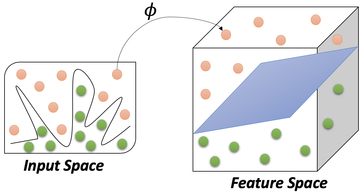
Figure 1: Kernel visualization from low dimension input space to high dimension feature space.

II Kernel Method

Traditional ML begins with a dataset of inputs $\mathcal{D}=\{x_{1},\cdots,x_{M}\}$ drawn from a set $\mathcal{X}$. The goal is to produce a predictive model that allows patterns to be discovered in yet to be observed data. Kernel methods use the inner product $K(x,x^{\prime})$ between any given two inputs $x,x^{\prime}\in\mathcal{X}$, as a distance measure to build predictive models that assist with representing characteristics of a data distribution.

Definition II.1.

Let $\mathcal{X}$ be a nonempty set, called the index set, and $\mathcal{H}$ by a Hilbert space of functions $\phi:\mathcal{X}\rightarrow\mathbb{R}$. Then $\mathcal{H}$ is called a reproducing kernel Hilbert space endowed with the dot product, $\bra{\cdot}\ket{\cdot}$, if there exists a function $k:\mathcal{X}\times\mathcal{X\rightarrow\mathcal{R}}$ with the two following properties: (i) $k$ has the reproducing property, i.e., $\bra{\phi}\ket{k(x,\cdot)}=\phi(x)$ for all $\phi\in\mathcal{H}$; (ii) $k$ spans $\mathcal{H}$ Scholkopf and Smola (2001).

Note that in particular $\bra{k(x,\cdot)}\ket{k(x^{\prime},\cdot)}=k(x,x^{\prime})=k(x^{\prime},x)$ guarantees symmetry of the arguments of $k$.

Theorem II.1.

Let $\phi:\mathcal{X}\rightarrow\mathcal{F}$ be a feature map. Kernel function can be defined as the inner product of two inputs mapped to some feature space by, $\mathbf{k}(x,x^{\prime})=\langle\phi(x),\phi(x^{\prime})\rangle$.

Proof.

The proof can be found in references Hofmann et al. (2008); Kübler et al. (2019). ∎

Theorem II.2.

Consider a feature mapping is $\phi:\mathcal{X}\rightarrow\mathcal{F}$ over some input set $\mathcal{X}$, which provide the basis to a complex kernel $\mathbf{k}(x,x^{\prime})=\langle\phi(x),\phi(x^{\prime})\rangle$ that is defined on $\mathcal{F}$. The associated reproducing kernel Hilbert space can be written as $\mathcal{R}_{\mathbf{k}}=\{f:\mathcal{X}\rightarrow\mathbb{C}\}$

$$f(x)=\langle w,\phi(x^{\prime})\rangle,$$ (1)

for all $w\in\mathcal{F}$ and $x\in\mathcal{X}$.

Proof.

The proof can be found in Hofmann et al. (2008) and . ∎

III Coherent State

A harmonic oscillator in quantum physics is described by the following Hamiltonian:

$$H=\hbar\omega\left(\hat{n}+\frac{1}{2}\right)$$ (2)

in which $\hbar$ is the Planck’s constant and $\omega$ is the angular frequency of the oscillator; the number operator $\hat{n}$ is described by annihilation and creation operators, i.e., $\hat{n}=\hat{a}^{\dagger}\hat{a}$. The Schörodinger equation gives the discrete energy eigenvalue:

$$H\ket{n}=E_{n}\ket{n},\ n=0,1,2,\cdots$$ (3)

in which eigenvalue $E_{n}=\hbar\omega(n+1/2)$ is associated by eigenstate $\ket{n}$. For simplicity, we consider $\hbar=1$ and $\omega=1$ in the rest of the paper.
A coherent state is the specific quantum state of the quantum harmonic oscillator, often described as a state which has dynamics most closely resembling the oscillatory behavior of a classical harmonic oscillator, for example see Ali et al. (2000).

Definition III.1.

A coherent state is defined as superposition of number state $\ket{n}$ as following:

$$\ket{\alpha}=e^{-|\alpha|^{2}/2}\sum_{n=0}^{\infty}\frac{\alpha^{n}}{\sqrt{n!}}\ket{n}$$ (4)

which number states satisfy $\bra{n}\ket{m}=\delta_{n,m}$, where $\delta_{n,m}$ is Kronecker delta.

Note that the inner product of two coherent states is given by:

$$\bra{\alpha}\ket{\beta}=e^{|\alpha-\beta|^{2}/2}$$ (5)

Lemma III.1.

A harmonic oscillator coherent state adheres the following:

1. It is obtained by operation of the displacement operator $D(\mathbf{\alpha})=\exp{\left(\alpha^{\ast}a^{\dagger}-\alpha a\right)}$ on a reference state: $|\alpha\rangle=D(\alpha)|0\rangle$, in which $\ket{\alpha}$ is given by the relation (4).

2. It is an eigenvector of the annihilation operator, $a|\alpha\rangle=\alpha|\alpha\rangle$.

3. It fulfills the minimum uncertainty relation, i.e., $\Delta(\mathbf{x})=\Delta(\mathbf{p})=1/\sqrt{2}$, where $\Delta(\mathbf{x})=\sqrt{\langle\mathbf{x}^{2}\rangle-\langle\mathbf{x}\rangle^{2}}$, where $\langle\mathbf{x}\rangle=\bra{\alpha}\mathbf{x}\ket{\alpha}$.

4. It is over-complete, $K(\alpha,\alpha^{\prime})=\bra{\alpha}\ket{\alpha^{\prime}}\neq\delta(\alpha-\alpha^{\prime})$, i.e., the equation (5), despite the fact that they fulfil the resolution of the identity, $\int d\mu(\mathbf{x})|\mathbf{x}\rangle\langle\mathbf{x}|=\mathbb{I}$, which leads to the following relation:

   $$\int d\mu(\mathbf{x})\langle\phi|\mathbf{x}\rangle\langle\mathbf{x}|\psi\rangle=\langle\phi|\psi\rangle.$$ (6)

Proof.

The proofs can be found in references Ali et al. (2000); Kübler et al. (2019). ∎

The latter, i.e., item $4$ of Lemma III.1, implies an arbitrary function can be expressible as a linear combination of kernel functions in a “reproducing Hilbert space” Combescure and Robert (2012). We should mention that the first above-mentioned property leads to define a displacement-type coherent states Ali et al. (2000), for generalized annihilation and creation operators. Moreover a Gazeau-Klauder coherent state is defined by the second property and fulfils the third property Ali et al. (2000). It should be noted that while the latter, i.e., resolution of the identity, fulfils all types of coherent states.

Recently Schuld and Killoran published a paper in which data is mapped into a feature space established by squeezed states Schuld and Killoran (2019). Squeezed states are states that saturate the Heisenberg uncertainty principle; additionally, the quadrature variance of position and momentum depend on a parameter, so-called squeezing parameter. The squeezing parameter causes the uncertainty to be squeezed one of its quadrature components, while stretched uncertainty for the other component, i.e. $\Delta(\mathbf{x})=\exp{2\zeta}/\sqrt{2}$ and $\Delta(\mathbf{p})=\exp{-2\zeta}/\sqrt{2}$, where $\zeta$ is the squeezing parameter. Therefore, the squeezing parameter controls uncertainty via a quadrature component, while the third and fourth properties of coherent states are preserved. However, as we mentioned, one of the well-known kernel functions in ML, the Radial Basis function (RBF), is defined by

$$K(\mathbf{x},\mathbf{x}^{\prime};\sigma)=\exp{\left(-||\mathbf{x}-\mathbf{x}^{\prime}||^{2}/2\sigma^{2}\right)},$$ (7)

where $\mathbf{x}$ and $\mathbf{x}^{\prime}$ are two sample elements, and $\sigma$ is understood as a free parameter. However, drawing a comparison between relations (5) and (7), inspires someone to interpret the RBF as an inner product of two coherent states. This interpretation opens the door to define new kernels and consequently improve the kernel method Kübler et al. (2019).

IV Non-linear Coherent State

As mentioned before, some efforts have been devoted to study possible generalization of the quantum harmonic oscillator algebra Man’ko et al. (1997). A deformed algebra is a non-trivial generalization of a given algebra through the introduction of one or more deformation parameters, such that, in a certain limit of the parameters, the non-deformed algebra can be recovered.

A particular deformation of the W-H algebra led to the notion of $f$-deformed oscillator Man’ko et al. (1997). An $f$-deformed oscillator is a non-harmonic system where its dynamical variables (creation and annihilation operators) are constructed from a non-canonical transformation through

$$\hat{A}=\hat{a}f(\hat{n})=f(\hat{n}+1)\hat{a},$$ (8)

$$\hat{A}^{{\dagger}}=f^{{\dagger}}(\hat{n})\hat{a}^{{\dagger}}=\hat{a}^{{\dagger}}f^{{\dagger}}(\hat{n}+1).$$ (9)

where $f(\hat{n})$ is called deformation function by which non-linear properties of this system are governed. An $f$-deformed oscillator is characterized by a Hamiltonian of the harmonic oscillator form,

$$\hat{H}=\frac{\omega}{2}(\hat{A}\hat{A}^{{\dagger}}+\hat{A}^{{\dagger}}\hat{A}),$$ (10)

where $\hat{A}$ and $\hat{A}^{{\dagger}}$ are given in equations (8) and (9). In this Hamiltonian, $\omega$ is frequency of harmonic oscillator and $\hslash=m=1$. The deformed operators satisfy the following commutation relation

$$[\hat{A},\hat{A}^{{\dagger}}]=(\hat{n}+1)f^{2}(\hat{n}+1)-\hat{n}f^{2}(\hat{n}).$$ (11)

Relations (8) and (9) give eigenvalues of the Hamiltonian (10) as follows:

$$E_{n}=\frac{\omega}{2}((n+1)f^{2}(n+1)+nf^{2}(n)).$$ (12)

It is worth to mention that by approaching deformation function into $1$, i.e., $f(n)\rightarrow 1$, the non-deformation energy eigenvalues, $E_{n}=\omega(n+\frac{1}{2})$, and the non-deformed commutation relation $[\hat{a},\hat{a}^{{\dagger}}]=1$ are recovered. However, similar to the harmonic oscillator, it is possible to construct coherent states for the $f$-deformed oscillator. The non-linear transformation of the creation and annihilation operators leads naturally to the notion of non-linear coherent states or $f$-coherent states Dehdashti et al. (2015a, 2013a, 2013b, b).

Definition IV.1.

Non-linear coherent states are defined as the right-hand eigenstates of the deformed annihilation operator $\hat{A}$ as follows Ali et al. (2000):

$$\hat{A}|\alpha\rangle_{f}=\alpha|\alpha\rangle_{f}.$$ (13)

From equation (13) one can obtain an explicit form of the non-linear coherent states in the number state representation as,

$$|\alpha\rangle_{f}=\frac{1}{\mathcal{N}}\sum_{n}^{M}\frac{\alpha^{n}}{\sqrt{n![f(n)]!}}|n\rangle,$$ (14)

where $M$ can be finite, or infinite (corresponding to finite or infinite dimensional Hilbert space), $\alpha$ is a complex number and $[f(n)]!=\prod_{i=0}^{n}f(i)$, with $[f(0)]!=1$; the normalization factor $\mathcal{N}$ is given by

$$\mathcal{N}=\left(\sum_{n=0}^{M}\frac{|\alpha|^{2n}}{n![f(n)]!}\right)^{-1/2}.$$ (15)

Therefore, based on the definition II.1, we can define a kernel as the following:

Definition IV.2.

By mapping multi-dimensional input set $\mathbf{x}=(x_{1},\cdots,x_{N})^{T}\in\mathbb{R}^{N}$ into non-linear coherent states, defined by the relation (14), so that they are fulfilled with resolution of the identity, a feature space is defined as

$$\phi:(x_{1},\cdots,x_{N})\rightarrow|x_{1}\rangle_{f}\otimes|x_{2}\rangle_{f}\otimes\cdots\otimes|x_{N}\rangle_{f}.$$

In addition, the associated kernel is obtained by the inner product as the following:

$$K(\mathbf{x},\mathbf{x^{\prime}})=\prod_{i=1}^{N}\ {}_{f}\langle x_{i}|x_{i}^{\prime}\rangle_{f},$$ (16)

in which

$${}_{f}\langle x_{i}|x_{i}^{\prime}\rangle_{f}=\frac{1}{\mathcal{N}^{2}}\sum_{n=0}^{M}\frac{(x_{i}x_{i}^{\prime})^{m}}{m![f(m)]!}.$$ (17)

IV.1 Non-Linear coherent state of an oscillator with variable mass

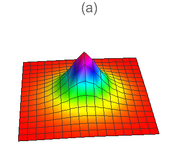
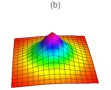
Figure 2: Schematic shape of the kernel function (22) for $k=-0.001$ and $k=-0.5$ in plots (a) and (b), respectively. The input $x$ is fixed at $(0,0)$ and $x^{\prime}$ is varied.

The quantum version of a non-linear oscillator Hamiltonian with variable mass is given by Tchoffo et al. (2019)

$$H=\frac{1}{2\lambda}\left[-(1+\delta^{2}x^{2})\frac{d^{2}}{dx^{2}}-2\delta^{2}x\frac{d}{dx}+\frac{\lambda^{2}x^{2}}{1+\delta^{2}x^{2}}\right]$$ (18)

in which where $\lambda$ is a real parameter and $\delta$ is constant that measures the force of the nonlinearity of the oscillator. By using ladder operators, one can define a non-linear coherent state as the following:

$$\ket{x}=\frac{1}{\mathcal{N}(x)}\sum_{n=0}^{\infty}\frac{x^{n}}{\rho_{n}}\ket{n}$$ (19)

in which $\rho_{n}=n!(-k)^{n}(2-1/k)_{n}$, which $(u)_{n}=u(u-1)\cdots(u+n-1)$ represents the Pochhammer symbol, $k=\delta^{2}/2\lambda$ and normalization factor $\mathcal{N}(x)$ is given by

$$\mathcal{N}^{2}(x) = \sum_{n=0}^{\infty}\left(\frac{(1/k)^{n}}{n!(2-1/k)_{n}}\right)^{2}|x|^{2n}$$ (20)

$$= {}_{0}F_{3}(;1,2-1/k,2-1/k;|x/k|^{2})$$

which ${}_{0}F_{3}(;1,2-1/k,2-1/k;|x/k|^{2})$ is a generalized hyper-geometric function.
By considering a multi-dimensional input set in a data set of vectors $\mathbf{x}=(x_{1},\cdots,x_{N})^{T}\in\mathbb{R}^{N}$, one can define the joint state of $N$ deformed coherent states,

$$\phi:(x_{1},\cdots,x_{N})\rightarrow|x_{1},k\rangle\otimes|x_{2},k\rangle\otimes\cdots\otimes|x_{N},k\rangle.$$

Therefore, the kernel is defined as the following:

$$K(\mathbf{x},\mathbf{x^{\prime}})=\prod_{i=1}^{N}\langle x_{i};k|x_{i}^{\prime};k\rangle,$$ (21)

in which

$$\langle x_{i};k|x_{i}^{\prime};k\rangle=\frac{{}_{0}F_{3}(;1,2-1/k,2-1/k;x_{i}x_{i}^{\prime}/k^{2})}{\mathcal{N}(x)\mathcal{N}(x^{\prime})}$$ (22)

Figure 2 schematically illustrates the kernel function (22), for $k=-0.001$ and $k=-0.05$.

IV.2 Geometrical properties of associated Hilbert Space constructed by Non-linear coherent state

For understanding the rule of nonlinear parameter $k$, we will study the geometrical properties of above-mentioned feature spaces. We can define the line element of the feature space by using the Fubini-Study metric Bengtsson and Życzkowski (2017).

Definition IV.3.

A suitable metric between two Hilbert space vectors, e.g, $\ket{\psi}$ and $\ket{\phi}$, is defined by

$$d(\ket{\psi},\ket{\phi})=\min||\ket{\psi}-e^{i\alpha}\ket{\phi}||,\ 0\leq\alpha\leq 2\pi.$$ (23)

The infinitesimal form of this metric is given by the Fubini-Study metric:

$$ds^{2}=||d\ket{x}||^{2}-||\bra{x}d\ket{x}||^{2}.$$ (24)

The following gives the Fubini-Study metric of a non-Linear coherent state (19).

Theorem IV.1.

The Fubini-Study metric of a non-linear coherent state (19) is a surface with non-zero curvature with the following metric:

$$ds^{2}=\Omega(r)\left(dr^{2}+r^{2}d\phi^{2}\right),$$ (25)

in which

$$\Omega(r)=\frac{1}{2}\left[\frac{\partial^{2}_{r}\mathcal{N}(r)}{\mathcal{N}(r)}+\frac{\partial_{r}\mathcal{N}(r)}{r\mathcal{N}(r)}-\left(\frac{\partial_{r}\mathcal{N}(r)}{\mathcal{N}(r)}\right)^{2}\right].$$ (26)

with $\partial_{r}\equiv\frac{\partial}{\partial r}$.

Proof.

We consider the $x=re^{i\phi}$, using the definition (24), directly leads to the metric (25).
By using the definition of Christoffel symbol,

$$\Gamma_{ab}^{c}=\frac{1}{2}g^{cd}\left(\partial_{a}g_{bd}+\partial_{b}g_{ad}-\partial_{d}g_{ab}\right),\ a,b,c=r,\phi$$ (27)

with the Einstein summation rule, the non-zero Christoffel symbols are given by

$$\Gamma_{rr}^{r} = \frac{1}{2}\partial_{r}\ln\Omega(r),$$ (28)

$$\Gamma_{\phi\phi}^{r} = -\left(r+\frac{r^{2}}{2}\partial_{r}\ln\Omega(r)\right),$$ (29)

$$\Gamma_{\phi r}^{\phi} = \frac{1}{r}+\frac{1}{2}\partial_{r}\ln\Omega(r).$$ (30)

Hence, the non-zero Ricci tensors are given by,

$$R_{rr} = -\frac{1}{2}\left(\partial_{r}^{2}\ln\Omega(r)+\frac{1}{r}\partial_{r}\ln\Omega(r)\right)$$ (31)

$$R_{\phi\phi} = -\frac{r}{2}\left(\partial_{r}\ln\Omega(r)+r\partial_{r}^{2}\ln\Omega(r)\right)$$ (32)

Hence, the Ricci scalar, $R=g^{ab}R_{ab}$, is obtained as

$$R=-\Omega(r)^{-1}\left(\partial_{r}^{2}\ln\Omega(r)+\frac{1}{r}\partial_{r}\ln\Omega(r)\right)$$ (33)

∎

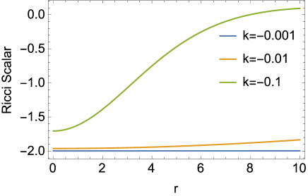
Figure 3: Ricci scalar of the Fubini-Study metric of a feature space constructed by a oscillator with variable mass as function of $r$, for different values of $k$.

It is worthwhile to note that the metric (25), which describes the feature space, is a surface that is conformal with flat space, that is conformally preserves angles, while lengths can be changed. In fact, this metric illustrates a two-dimensional curved space, depending on conformal function $\Omega(r)$. By considering the non-linear coherent state (19) and normalized coefficient (5), Fig. 3 represents the Ricci scalar for different values of $k$. This figure indicates that the feature space is a surface with negative curvature. Decreasing the value $k$ causes the Ricci curvature to increase. In other words, increasing value of $k$ causes the feature space and the associated kernel to approach a flat space and RBF kernel, respectively. Despite the fact that the feature space constructed on a non-linear coherent state is a non-zero curved space, RBF, which is constructed from a linear coherent state, is a kernel on flat space, with the zero Ricci scalar.

V Experimental Design

In the following, we empirically evaluate the KMNCS, i.e. the relation (21), RBF kernel, i.e., the relation (7), and the Squeezed kernel, given by

$$K_{Sq}=\prod_{i=1}\left[\frac{\sech c\sech c^{\prime}}{1-e^{i(x-x^{\prime})}\tanh c\tanh c^{\prime}}\right]^{1/2}.$$ (34)

SVM uses a kernel function to define a decision boundary for separating the data points. Generally, the hyper parameter $C$ in the Gaussian kernel is used to optimize the performance of SVM, as a cost function connected with mis-classifications of data points in feature space of the training set. We kept the hyperparameter $C=1$ as the optimal value.
In order to provide a comprehensive picture of the performance of the kernels, i.e., kernels (7), (34) and (21), noise was systematically applied to the input data. Applying noise implies adding it to the target variable. For example, if the noise parameter is say $0.2$, a standard deviation of $0.2$ would be observed (originating from Gaussian noise) in the output. When data points become inseparable due to noise, it becomes more challenging for the classifier to accurately classify the data points.
We have used synthetic datasets (simple toy datasets) which are commonly used to check the performance of kernels. The two datasets ($make\_moons$ and $make\_circles$) are taken from sklearn. There is some flexibility in regard to each dataset. Random noise can be introduced by adjusting different parameters for each dataset: the Moons dataset generates two half circles with the noise parameters affecting ’interleave’, the Circles dataset generates concentric circles also affected by ’interleave’ via the noise parameter. The decision region for class 1 is color-coded ’red’, and ’blue’ for class 0. We have also recorded differing values of $flip\_y$ which is an inbuilt parameter in $make\_classification$ ( Generate a random n-class classification problem) also from sklearn. A large $flip\_y$ supplements the noise effects, making accurate classification even more challenging. The $factor$ and $random\_state$ in the setting have also been recorded. We have divided the data into $60\%$ training set and $40\%$ test set. We have also used 5 fold cross validation during training in order to avoid overfitting problems. We have examined KMNCS using different values of $k$ in order to evaluate the classification performance and to understand how the decision boundaries are formed.

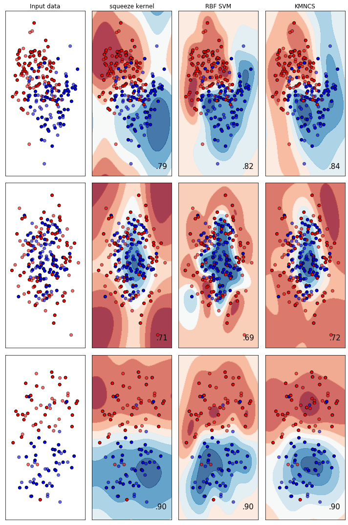
Figure 4: Kernel visualization (Squeezed, RBF kernels and KMNCS) for $k=-0.001$, while the noise is $0.4$ on both the make_moons and make_circles datasets.

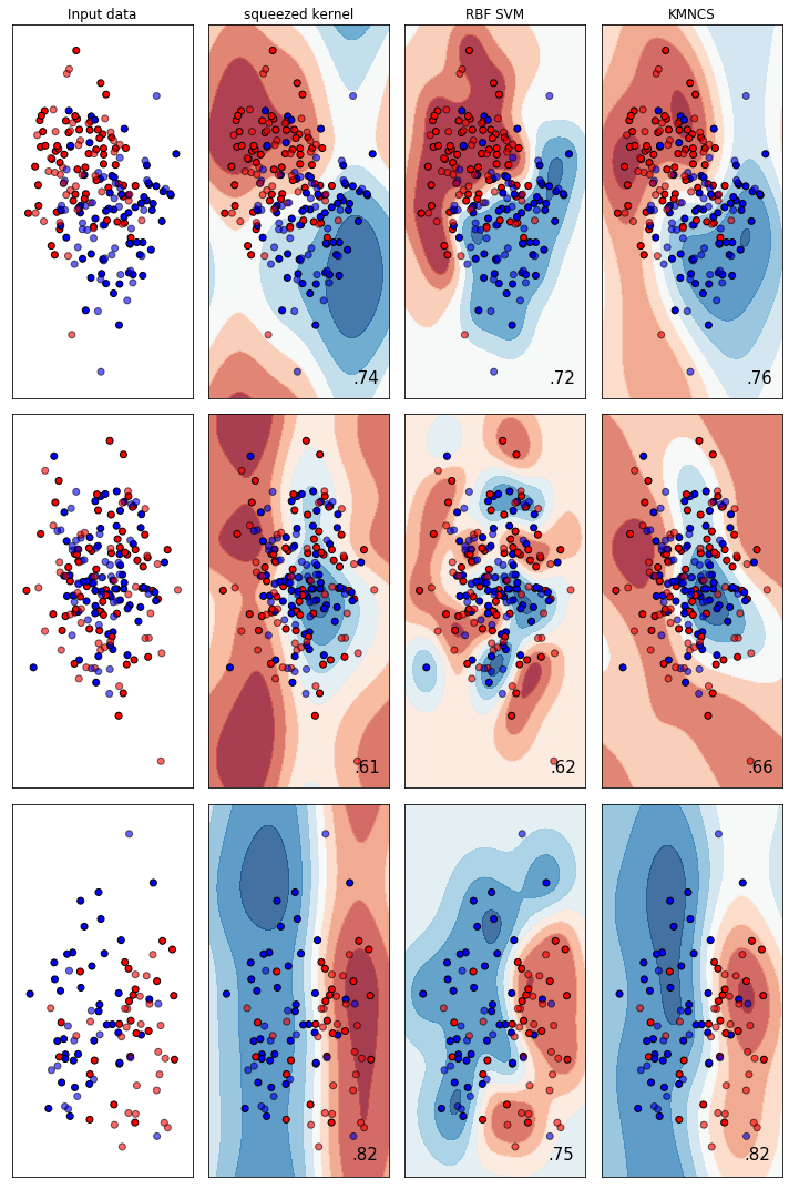
Figure 5: Kernel visualization (Squeezed, RBF, and KMNCS) for $k=-0.1$, while noise is $0.5$ on the make_moons dataset, and $0.7$ on the make_circles dataset.

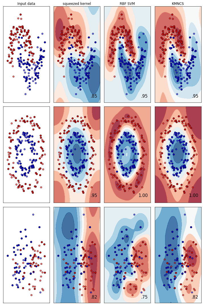
Figure 6: Kernel visualization (Squeezed, RBF, and KMNCS) for $k=-0.01$, while noise is $0.2$ on the make_moons dataset, and $0.1$ on make_circles dataset.

VI Results

The sklearn package includes a “fit” method that is used for informing the model by applying a training set. To compute the score by cross-validation of SVM, “cross_val_score” is used also from sklearn with a “5”-fold cross-validation.
As we can see from Table 1, KMNCS has been tested on several values of $k$. If we check the value of $k=-0.001$ with very low noise, i.e. $=0.1$, all the three kernels provide almost the same classification accuracy as can be seen in Figure 6 (Here the input data is separable and it is an easy task for the classifier to classify them). Interestingly, KMNCS has better performance than both baselines for both datasets when $k=-0.001$ and noise is $0.4$. This performance in the presence of such noise demonstrates effectiveness of KMNCS. The decision boundary is depicted in Figure 4.

When we increase the noise effect in the data, then classification becomes more challenging i.e., when noise is $0.5$ then KMNCS outperforms the squeezed and RBF kernel as can be seen in Figure 5. Note that it is possible to increase the accuracy of the classifier if we select $k=-0.01,-0.1$ with the same level of noise, that is $0.5$, as it can be seen in the Table 1. The KMNCS performance is deemed better than the baselines as data is inseparable (due to $50\%$ noise in the target variable). Again, where noise is $0.7$ and $k=-0.1$, then KMNCS provides better performance than the two baseline classifiers due to clean decision boundaries where data is separable, as can be seen in Figure 5.

We also tested on $3000$ samples as can be seen in Table 3. KMNCS outperforms both baselines which suggests it is effective on larger samples by producing clean decision boundaries.
There is a trade-off with decision boundaries and accuracy. It is possible to achieve even higher accuracy if we continue to modify $k$, however this may obscure the decision boundaries ( despite high accuracy scores), which could be related to bias and variance issues. We also computed the score without the cross validation set with the results presented in Table 2.

Table 1: Accuracy on Squeezed kernel, RBF, and KMNCS on the make_moon and make_circles datasets with the following parameters: n_samples=200, random_state=50, y_flip=0.2, factor=0.5, n_informative=2, 5-fold cross validation. Noise effects are introduced in the data to increase difficulty of accurate classification.

	Parameters	moons	circles
Squeezed Kernel	Noise=0.1	0.90	0.95
	Noise=0.2	0.85	0.86
	Noise=0.3	0.82	0.80
	Noise=0.4	0.79	0.71
	Noise=0.5	0.74	0.68
	Noise=0.7	0.62	0.61
RBF	Noise=0.1	0.99	1.0
	Noise=0.2	0.95	0.90
	Noise=0.3	0.89	0.80
	Noise=0.4	0.82	0.69
	Noise=0.5	0.72	0.64
	Noise=0.7	0.65	0.62
KMNCS	Noise=0.1, k=-0.001	0.97	1.0
	Noise=0.2, k=-0.001	0.95	0.88
	Noise=0.2, k=-0.01	0.95	0.89
	Noise=0.2, k=-0.1	0.94	0.88
	Noise=0.3, k=-0.001	0.90	0.79
	Noise=0.3, k=-0.01	0.90	0.79
	Noise=0.4, k=-0.001	0.84	0.72
	Noise=0.4, k=-0.01	0.84	0.72
	Noise=0.5, k=-0.001	0.75	0.68
	Noise=0.5, k=-0.01	0.76	0.69
	Noise=0.5, k=-0.1	0.76	0.70
	Noise=0.7, k=-0.001	0.64	0.62
	Noise=0.7, k=-0.01	0.62	0.62
	Noise=0.7, k=-0.1	0.65	0.66

Table 2: Accuracy on same parameters from Table 1 without cross validation

	Parameters	moons	circles
Squeezed Kernel	Noise=0.2	0.90	0.94
	Noise=0.5	0.75	0.70
	Noise=0.7	0.68	0.56
RBF	Noise=0.2	0.96	0.90
	Noise=0.5	0.76	0.64
	Noise=0.7	0.70	0.54
KMNCS	Noise=0.2, k=-0.001	0.99	0.93
	Noise=0.5, k=-0.001	0.75	0.66
	Noise=0.7, k=-0.001	0.71	0.54

Table 3: Accuracy on 3000 samples with same parameters from Table 1 as well as 5-fold cross validation

	Parameters	moons	circles
Squeezed Kernel	Noise=0.5	0.81	0.65
	Noise=0.8	0.72	0.55
	Noise=1.0	0.68	0.52
RBF	Noise=0.5	0.81	0.64
	Noise=0.8	0.73	0.54
	Noise=1.0	0.68	0.51
KMNCS	Noise=0.5, k=-0.1	0.82	0.65
	Noise=0.5, k=-0.01	0.81	0.65
	Noise=0.8, k=-0.1	0.73	0.56
	Noise=1.0, k=-0.1	0.69	0.53

VII Discussion

With respect to the general behaviour of KMNCS, it can be said that the kernel is conducive to forming large decision boundaries, which is a major point of contrast when considering the RBF kernel, as evident in Figure 4,5. As previously mentioned, the hyper-parameter $C$ can be used to optimise an SVM classifier, as a cost function associated with mis-classification of elements in feature spaces of the ’training’ set. It implies the maximisation of $C$ tightens decision boundaries (so called ’hard’ margins), and was introduced by Boser et al. Boser et al. (1992). In later work, ’hard’ margins were found to fail on even slightly inseparable data. As a solution, Schiilkop et al. (1995) introduced a meaningful technique for the minimisation of $C$ that was found to enlarge the space covered by decision boundaries (’soft’ margins). While this has largely benefited the field of SVM in contention with other classification techniques, the trade-off is that significantly ’soft’ margins fail to classify data entirely - formally known as over-generalisation, large decision boundaries (as produced by the Squeezed kernel) become non-representative of the data. As a result, the objective is to minimise the hyper-parameter $C$, while maintaining the highest possible classification. Relating this back to the findings of this paper, the topological structure of the KMNCS is reminiscent of Ref. Boser et al. (1992), surprisingly in cases of sparse data ( in this case the sparse $make\_moons$ dataset), without concern for $C$.

VIII Conclusions and Remarks

In this paper, we mapped datasets into non-linear coherent states, as a non-linear feature space, constructed by a complex Hilbert space. We showed that the RBF kernel is recovered when data is mapped to a complex Hilbert space represented by coherent states. Therefore, non-linear coherent states can be considered as natural generalized candidates for formalizing kernels. In addition, by considering the non-linear coherent states of a quantum oscillator with variable mass, we proposed a kernel function based on generalized hypergeometric functions. This idea suggests a method for obtaining a generalized kernel function which can be expressed by orthogonal polynomial functions on the one hand, and opens a new door for using quantum formalism to specify quantum algorithms in continuous variable quantum computing, on the other. In addition, we studied the geometrical properties of the surface in which the kernel lives. We indicated that the feature space of a non-linear coherent state is a non-zero curved space, despite the fact that the RBF kernel lives on feature space which is flat. This method can potentially open a door for studying the impact of general curved space on the machine learning methods more generally, and the problem of classification more specifically.
More generally, this research has demonstrated how quantum approaches to machine learning may prove beneficial. In practical usage, machine learning applications of quantum theory have begun involving developments of physical circuitry Havlíček et al. (2019). These contributions have begun to realise the quantum processing components required to build quantum computational devices designed solely for feature classification. It is inspiring to think that eventually, SVM classification may ( with the assistance of quantum theory) be computed substantially faster than ever before.