Power-efficiency-fluctuations trade-off in steady-state heat engines:
The role of interactions

Abstract

We consider the quality factor $\mathcal{Q}$, which quantifies the trade-off between power, efficiency, and fluctuations in steady-state heat engines modeled by dynamical systems. We show that the nonlinear scattering theory, both in classical and quantum mechanics, sets the bound $\mathcal{Q}=3/8$ when approaching the Carnot efficiency. On the other hand, interacting, nonintegrable and momentum-conserving systems can achieve the value $\mathcal{Q}=1/2$, which is the universal upper bound in linear response. This result shows that interactions are necessary to achieve the optimal performance of a steady-state heat engine.

Introduction.- Understanding the bounds that a heat engine must obey is of key importance both for basic science and for technological development. Ideally, a heat engine should work with efficiency $\eta$ close to the Carnot efficiency $\eta_{C}$, deliver large power $P$, and have small power fluctuations $\Delta_{P}$. The Carnot limit is intuitively associated with infinitely slow engines, so that the output power vanishes. On the other hand, the second law of thermodynamics by itself does not forbid an engine operating at the Carnot efficiency with a finite output power Benenti2011 . Such a dream engine was denied in models with inelastic scattering Saito2011 ; Sanchez2011 ; Horvat2012 ; Vinitha2013 ; Brandner2013a ; Brandner2013b ; Brandner2015 ; Yamamoto2016 and for two-terminal systems on the basis of symmetry considerations for the Onsager kinetic coefficients Luo2020 . Moreover, for systems described as Markov processes, the bound $P\leq A(\eta_{C}-\eta)$ was proven Saito2016 , with $\eta_{C}=1-T_{R}/T_{L}$, $T_{L}$ and $T_{R}$ ($T_{L}>T_{R}$) being the temperatures of the hot and the cold reservoir, respectively, and $A$ a system-specific constant. On the other hand, $A$ may diverge when approaching the Carnot efficiency Allahverdyan2013 ; Shiraishi2015 ; Campisi2016 ; Koning2016 ; Polettini2017 ; Lee2017 , for instance, when the engine working fluid is at the verge of a phase transition, and therefore the Carnot efficiency may be approached at finite power. However, fluctuations make impractical such engines Holubev2017 .

On the base of thermodynamic uncertainty relations Barato2015 ; Gingrich2016 ; Seifert2019 ; Horowitz2020 for the work current (i.e., for the power delivered by the engine), a trade-off encompassing efficiency, power, and fluctuations has been proven by Pietzonka and Seifert Pietzonka2018 , for a large class of steady-state classical stochastic heat engines with time-reversal symmetry. Such class includes engines with a discrete set of internal states described by thermodynamically consistent rate equations, and continuous systems modeled with an overdamped Langevin dynamics. The bound reads

$$\mathcal{Q}\equiv P\frac{\eta}{\eta_{C}-\eta}\frac{k_{B}T_{R}}{\Delta_{P}}\leq\frac{1}{2},$$ (1)

where $k_{B}$ is the Boltzmann constant and the power fluctuations are measured by footnote_DeltaP

$$\Delta_{P}=\lim_{t\to\infty}[P(t)-P]^{2}t,$$ (2)

where $P(t)$ is the mean delivered power up to time $t$.

In this paper, at difference from the above stochastic thermodynamics approach, we examine for purely dynamical models the upper bound to the quality factor $\mathcal{Q}$. We focus on the most desirable regime for a heat engine, i.e., when approaching the Carnot efficiency at the largest possible output power. We first find a general solution to this problem for systems that can be modeled by the nonlinear scattering theory. That is, for noninteracting systems or more generally for systems in which interactions can be treated at a mean-field Hartree level. In this case we prove that the quality factor $\mathcal{Q}<3/8$, and that the limit value $\mathcal{Q}=3/8<1/2$ is only achieved for $\eta\to\eta_{C}$. Scattering theory sets therefore a stronger bound to the quality factor $\mathcal{Q}$ than Eq. (1). We stress that the above results are valid both in classical and in quantum mechanics. We then consider the class of interacting, non-integrable momentum-conserving systems. This is, to our knowledge, the only class of interacting dynamical systems which is known to achieve, at the thermodynamic limit, the Carnot efficiency Benenti2013 ; Benenti2014 ; Chen2015 . We show in a concrete example of a nonintegrable gas of elastically colliding particles that such systems saturate the bound $\mathcal{Q}=1/2$. This value is achieved in the tight-coupling limit, where the Onsager matrix of kinetic coefficients becomes singular.

Bound from scattering theory.- For concreteness, hereafter we consider thermoelectric transport, even though our results could be equally applied to other examples of steady-state conversion of heat to work, like thermodiffusion. In the Landauer-Büttiker quantum scattering theory, the electrical current, flowing from the left to the right reservoir, reads

$$J_{e}=\frac{e}{h}\int_{-\infty}^{\infty}d\epsilon\,{\cal T}(\epsilon)\,[f_{L}(\epsilon)-f_{R}(\epsilon)],$$ (3)

where $e$ is the electron charge, $h$ the Planck constant, ${\cal T}(\epsilon)$ the transmission probability for a particle with energy $\epsilon$ to transit from one end to another of the system ($0\leq{\cal T}(\epsilon)\leq 1$), and $f_{\alpha}(\epsilon)=\{1+\exp[(\epsilon-\mu_{\alpha})/k_{B}T_{\alpha}]\}^{-1}$ is the Fermi distribution function for reservoir $\alpha$ ($\alpha=L,R$), at temperature $T_{\alpha}$ and electrochemical potential $\mu_{\alpha}$ footnote_modes . The heat current that flows into the system from reservoir $\alpha$ is

$$J_{h,\alpha}=\frac{1}{h}\int_{-\infty}^{\infty}d\epsilon\,(\epsilon-\mu_{\alpha})\,{\cal T}(\epsilon)\,[f_{L}(\epsilon)-f_{R}(\epsilon)].$$ (4)

The output power $P=(\Delta V)J_{e}$, where $\Delta V=\Delta\mu/e$ is the applied voltage, with $\Delta\mu=\mu_{R}-\mu_{L}>0$. The efficiency of heat to work conversion is given by $\eta=P/J_{h,L}$, with $P,J_{h,L}>0$. The transmission function which maximizes the efficiency for a given power is a boxcar function, ${\cal T}(\epsilon)=1$ for $\epsilon_{0}<\epsilon<\epsilon_{1}$ and ${\cal T}(\epsilon)=0$ otherwise Whitney2014 ; Whitney2015 . Here $\epsilon_{0}=\Delta\mu/\eta_{C}$ is obtained from the condition $f_{L}(\epsilon_{0})=f_{R}(\epsilon_{0})$ and $\epsilon_{1}$ can be determined numerically by solving the equation $\epsilon_{1}=\Delta\mu J_{h,L}^{\prime}/P^{\prime}$, where the prime indicates the derivative over $\Delta\mu$ for fixed ${\cal T}$ (this equation is transcendental since $J_{h,L}$ and $P$ depend on $\epsilon_{1}$). The maximum achievable power $P_{\rm max}$ is obtained when $\epsilon_{1}\to\infty$ and is given by $P_{\rm max}\approx 0.317\,k_{B}^{2}(\Delta T)^{2}/h$, with $\Delta T=T_{L}-T_{R}>0$. In the limit $\epsilon_{1}\to\epsilon_{0}$, known as delta-energy filtering mahan ; linke1 ; linke2 , $P\to 0$ and $\eta\to\eta_{C}$.

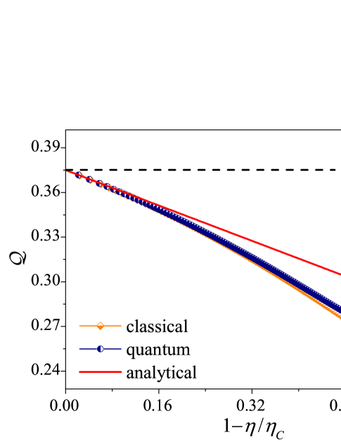
Figure 1: Quantum and classical quality factor $\mathcal{Q}$ based on the scattering theory. For $\eta$ close to $\eta_{C}$, numerical results are in excellent agreement with the analytical formula (6) up to the linear term (red solid line). The dashed line indicates the bound $\mathcal{Q}=3/8$ for reference. Parameter values adopted in simulations are $T_{L}=1$, $T_{R}=0.9$, $\mu_{L}=0$. For any value of power, $\mu_{R}=\Delta\mu$ is determined in the optimization procedure described in the text. Here we use units such that $k_{B}=e=h=1$.

The power fluctuations can be computed from the Levitov-Lesovik cumulant generating function Levitov1993 ; Nazarov2009 ; Segal2019 . For the above boxcar function, we obtain

$$\Delta_{P}=\frac{(\Delta\mu)^{2}}{h}\int_{\epsilon_{0}}^{\epsilon_{1}}d\epsilon\,[f_{L}(\epsilon)+f_{R}(\epsilon)-f_{L}^{2}(\epsilon)-f_{R}^{2}(\epsilon)].$$ (5)

Using the above defined expressions for $\eta$, $P$, and $\Delta_{P}$, we can compute the quality factor $\mathcal{Q}$. As detailed in the supplemental material supp , we can expand $\mathcal{Q}$ close to the Carnot efficiency, that is, for $1-\eta/\eta_{C}\ll 1$. We then obtain the analytical result

$$\mathcal{Q}=\frac{3}{8}-\frac{9}{128}\frac{T_{L}+T_{R}}{T_{R}}\left(1-\frac{\eta}{\eta_{C}}\right)+\mathcal{O}\left[\left(1-\frac{\eta}{\eta_{C}}\right)^{2}\right].$$ (6)

When going far from the Carnot limit, the dependence of $\mathcal{Q}$ on efficiency can be computed numerically. The results are shown in Fig. 1, for the optimal boxcar function, which maximizes efficiency for any value of power. We can see that $\mathcal{Q}<3/8$ for any value of $\eta$, the value $\mathcal{Q}=3/8$ being obtained only for $\eta=\eta_{C}$ (correspondingly, $P=0$). A similar analysis can be performed in the classical case supp , and for the optimal boxcar function Luo2018 expansion (6) is still valid. As shown in Fig. 1, classical and quantum $\mathcal{Q}$ differ at higher orders, with the quantum quality factor slightly larger than the classical one.

Momentum-conserving systems.- The above results raise two interesting questions: (i) Is it possible to find interacting systems which may overcome the scattering theory bound $\mathcal{Q}=3/8$? (ii) Is it possible to approach or even overcome bound (1), $\mathcal{Q}=1/2$, when approaching the Carnot efficiency? To address this question, we consider non-integrable momentum-conserving systems, for which the Carnot limit can be achieved at the thermodynami limit Benenti2013 ; Benenti2014 ; Chen2015 . We perform nonequilibrium simulations, with the momentum-conserving system (specifically, a classical one-dimensional diatomic gas of elastically colliding particles Benenti2013 ) in contact with two reservoirs at different temperatures and electrochemical potentials, which maintain stationary coupled energy and particle flows. In our simulations, particles are absorbed whenever they hit a reservoir, while the two reservoirs inject particles with rates and energy distributions determined by their temperatures and electrochemical potentials reservoir .

From our numerical simulations, we can determine the charge and heat currents, and consequently power, efficiency, and fluctuations. In Fig. 2, we compute the trade-off $\mathcal{Q}$ for different system sizes $L$. Note that these curves have two values for a given value of efficiency $\eta$, as they are obtained by changing $\Delta\mu$ from zero, where $\eta=0$, up to the stopping value, where the electrochemical potential difference becomes too high to be overcome by the temperature difference, and again $\eta=0$. The branch with higher values of $\mathcal{Q}$ corresponds to the lower values of $\Delta\mu$. Note that the scattering theory bound $\mathcal{Q}=3/8$ is overcome, up to higher values of the efficiency as the system size increases. At the same time, bound (1), $\mathcal{Q}=1/2$, is approached closer and closer.

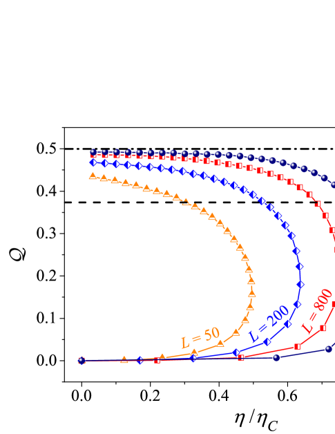
Figure 2: Quality factor versus efficiency for a one-dimensional diatomic gas of elastically colliding particles of masses $m=1$ and $M=3$ with $T_{L}=1.05$, $T_{R}=0.95$, $\mu_{L}=-\Delta\mu/2$, and $\mu_{R}=\Delta\mu/2$. The system size $L$ is equal to the mean number of particles inside the system. The dashed and the dot-dashed line indicate the bound $\mathcal{Q}=3/8$ and $\mathcal{Q}=1/2$, respectively. We set $k_{B}=e=1$.

Linear response results.- For a given temperature difference $\Delta T=T_{L}-T_{R}$, the gradient $|\nabla T|=\Delta T/L$ decreases with the system size $L$. We can then apply the linear response theory in the large-$L$ regime, which is the most interesting one in our model, as the Carnot efficiency is achieved when $L\to\infty$. Within linear response, the charge and heat currents (from the left to the right reservoir) are given by Callen ; Groot ; Benenti2017

$$\left(\begin{array}[]{c}J_{e}\\ J_{h}\end{array}\right)=\left(\begin{array}[]{cc}L_{ee}&L_{eh}\\ L_{he}&L_{hh}\end{array}\right)\left(\begin{array}[]{c}\mathcal{F}_{e}\\ \mathcal{F}_{h}\end{array}\right),$$ (7)

where $\mathcal{F}_{e}=-\nabla[\mu/(ek_{B}T)]$ and $\mathcal{F}_{h}=\nabla[1/(k_{B}T)]$ are the thermodynamic forces and $L_{ij}$ ($i,j=e,h$) the Onsager kinetic coefficients, which obey, for systems with time-reversal symmetry, the Onsager reciprocal relation $L_{eh}=L_{he}$. The matrix of the kinetic coefficients is known as the Onsager matrix $\mathbb{L}$. The second law of thermodynamics imposes $L_{ee}\geq 0$, $L_{hh}\geq 0$, and $\det\mathbb{L}\geq 0$.

We consider a generic linear combination of the currents, $J_{\bf c}=\sum_{\alpha}c_{\alpha}J_{\alpha}={\bf c}^{T}\mathbb{L}{\bm{\mathcal{F}}}$, where ${\bm{\mathcal{F}}}$ is the vector of thermodynamic forces. Thermodynamic uncertainty relations are saturated when ${\bf c}\parallel{\bm{\mathcal{F}}}$ on the orthogonal complement of the kernel of $\mathbb{L}$ Macieszczak2018 . In nonintegrable momentum-conserving systems, $\mathbb{L}$ becomes singular in the thermodynamic limit, where the Onsager matrix becomes singular (a condition known as tight-coupling limit, for which the Carnot efficiency is achievable). In this limit, the orthogonal complement of the kernel of $\mathbb{L}$ is one-dimensional, and therefore the thermodynamic uncertainty relations are saturated for all ${\bf c}$. In particular, bound (1) is saturated. In contrast, for finite system sizes the Onsager matrix is positive and the only current such that ${\bf c}\parallel{\bm{\mathcal{F}}}$ is the entropy production rate $\dot{S}=\mathcal{F}_{e}J_{e}+\mathcal{F}_{h}J_{h}$. Since power fluctuations $\Delta_{P}$ are proportional to charge fluctuations and not to $\dot{S}$, it follows that bound (1) is saturated only at the thermodynamic limit.

The validity of using linear response to interpret our numerical data is numerically confirmed by Fig. 3. For different system sizes, $\eta/\eta_{C}$ is shown as a function of $P/P_{\rm max}$, where $P_{\rm max}$ is the maximum power obtained when $\Delta\mu$ is varied from zero, where $P=0$, up to the stopping value, where again $P=0$. In the same figure, we also show the linear response result in the tight-coupling limit Benenti2017 :

$$\frac{\eta}{\eta_{C}}=\frac{P/P_{\rm max}}{2(1\pm\sqrt{1-P/P_{\rm max}})}.$$ (8)

Moreover, we rewrite bound (1) as

$$\frac{\eta}{\eta_{C}}\leq\frac{1}{1+2Pk_{B}T_{R}/\Delta_{P}}$$ (9)

and in the same figure we show the right-hand side of this inequality for the numerically computed values of power and fluctuations at the largest available system size, $L=3200$. Numerical results, however, suggest that the upper bound (9) does not depend on the system size. The tendency to saturate this bound when increasing the system size is clearly seen in Fig. 3. The excellent agreement between linear response expectations in the tight-coupling limit and the numerically computed upper bound on efficiency for given power and fluctuations, shows that linear response theory provides a satisfactory explanation of our results.

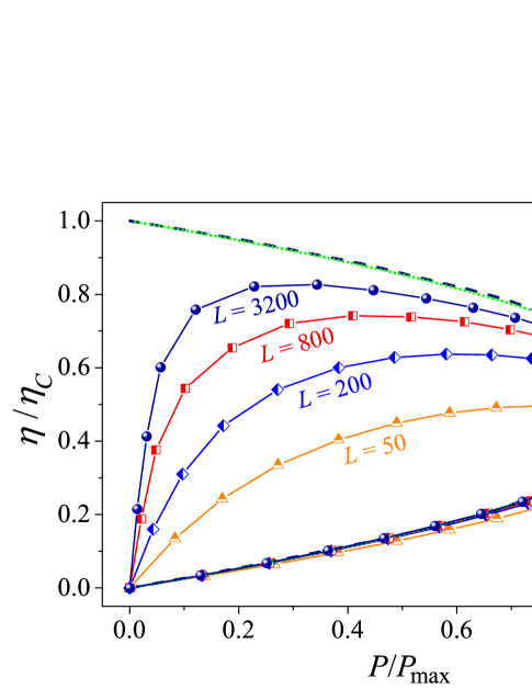
Figure 3: The same as Fig. 2 but for efficiency versus power for the diatomic gas model. The linear response prediction (8) in the tight-coupling limit (green dotted curve) and the upper bound (9) (blue dashed curve) are also shown.

Discussion and conclusions.- We have shown that for steady-state heat engines the power-efficiency-fluctuations trade-off $\mathcal{Q}\leq 3/8$ within the scattering theory, the upper bound $\mathcal{Q}=3/8$ being saturated at the Carnot efficiency. These conclusions hold both in classical and in quantum mechanics. On the other hand, interacting nonintegrable momentum-conserving systems may overcome this limit and saturate the linear-response upper bound $\mathcal{Q}=1/2$. This value is obtained in the tight-coupling limit, when the Onsager matrix becomes singular and the Carnot limit can be achieved. From the viewpoint of thermoelectric transport, our results confirm the relevance of the figure of merit $ZT=L_{eh}^{2}/\det\mathbb{L}$ Benenti2017 : Not only the Carnot efficiency can be achieved at the tight-coupling limit $ZT\to\infty$, but also the power-efficiency-fluctuations bound $\mathcal{Q}=1/2$ is saturated in the same limit. The trade-off $\mathcal{Q}$ could be investigated experimentally in the context of cold atoms, where a thermoelectric heat engine with high $ZT$ has already been demonstrated, both for weakly Brantut2013 and strongly interacting particles Husmann2018 .

Our analysis does not include the effects of a magnetic field. However, for two-terminal systems our conclusions would not change. Indeed, the scattering-theory bound discussed in this paper is the same, irrespective of whether time-reversal symmetry is broken by an external magnetic field or not. Moreover, the Onsager matrix obeys the reciprocal relation $L_{eh}=L_{he}$ for interacting systems, even in presence of a generic magnetic field Luo2020 . The effects of a magnetic field on thermoelectric efficiency were investigated in systems with three or more terminals, which mimic inelastic scattering events, but in that case it was not possible to achieve the Carnot efficiency Horvat2012 ; Vinitha2013 ; Brandner2013a ; Brandner2013b ; Brandner2015 ; Yamamoto2016 . It remains therefore as an interesting question whether the linear-response bound $\mathcal{Q}=1/2$ may be overcome by a, classical or quantum, interacting model when approaching the Carnot limit. More generally, we wonder whether stringent bounds from the scattering theory also apply for periodically driven systems.

We acknowledge support by the NSFC (Grant No. 11535011) and by the INFN through the project QUANTUM.

Appendix A Supplemental Material

Here we provide more details on the derivation of the quality factor $\mathcal{Q}$ from the scattering theory, for efficiency close to the Carnot efficiency, Eq. (6) of the main text. Hereafter we set $k_{B}=e=h=1$. In the limit $\delta\equiv\epsilon_{1}-\epsilon_{0}\to 0^{+}$, the power $P\sim\delta^{2}$, the deviation from the Carnot efficiency $\eta_{C}-\eta\sim\delta$, the fluctuations $\Delta_{P}\sim\delta$, so that the trade-off factor $\mathcal{Q}$ goes to a constant when $\delta\to 0^{+}$. More precisely, for the power we obtain

$$P=(\Delta V)\left[{\rm sech}\left(\frac{\Delta V}{2\Delta T}\right)\right]^{2}\frac{\Delta T}{8T_{L}T_{R}}\,\delta^{2}+\mathcal{O}(\delta^{3}),$$ (10)

where in the limit $\delta\to 0^{+}$ the voltage $\Delta V=\alpha\Delta T$ Whitney2015 , with $\alpha\approx 3.24$, the root of the transcendental equation

$$\alpha\tanh\left(\frac{\alpha}{2}\right)=3.$$ (11)

We can then rewrite the power as

$$P=\frac{\alpha(\Delta T)^{2}}{4(1+\cosh\alpha)T_{L}T_{R}}\,\delta^{2}+\mathcal{O}(\delta^{3}).$$ (12)

Similarly, we obtain the heat current that flows from the hot reservoir,

$$J_{h,L}=\frac{\alpha\Delta T}{4(1+\cosh\alpha)T_{R}}\,\delta^{2},+\mathcal{O}(\delta^{3}),$$ (13)

and the efficiency

$$\eta=\eta_{C}-\frac{2\eta_{C}}{3\alpha T_{L}}\,\delta+\mathcal{O}(\delta^{2}).$$ (14)

To compute power fluctuations, we use the formula Segal2019

$$\Delta_{P}=(\Delta V)^{2}\int_{-\infty}^{+\infty}d\epsilon({\cal T}(\epsilon)\{f_{L}(\epsilon)[1-f_{L}(\epsilon)]$$

$$+f_{R}(\epsilon)[1-f_{R}(\epsilon)]\}+{\cal T}(\epsilon)[1-{\cal T}(\epsilon)][f_{L}(\epsilon)-f_{R}(\epsilon)]^{2}),$$ (15)

which reduces to Eq. (5) of the main paper for the boxcar transmission function we are considering. Upon expansion for small $\delta$, we obtain

$$\Delta_{P}=\frac{\alpha^{2}(\Delta T)^{2}}{1+\cosh\alpha}\,\delta+\mathcal{O}(\delta^{2}).$$ (16)

Finally, we derive

$$\mathcal{Q}=\frac{3}{8}-\frac{T_{L}+T_{R}}{64T_{L}T_{R}}\frac{3}{\alpha}\,\delta+\mathcal{O}(\delta^{2}),$$ (17)

which reduces to Eq. (6) of the main text after inverting the relation between efficiency and width of the transmission window:

$$\delta=\frac{3}{2}\,\alpha T_{L}\left(1-\frac{\eta}{\eta_{C}}\right)+\mathcal{O}\left[\left(1-\frac{\eta}{\eta_{C}}\right)^{2}\right].$$ (18)

In the classical case, the Boltzmann distribution function $f_{\alpha}^{(B)}(\epsilon)=\exp[-(\epsilon-\mu_{\alpha})/T_{\alpha}]$ ($\alpha=L,R$) is considered rather than the Fermi distribution function in the calculation of $J_{e}$ and $J_{h,\alpha}$ Saito2010 ; Luo2018 . Moreover, the power fluctuations are given by Gaspard2013 ; Brandner2018

$$\Delta_{P}=(\Delta V)^{2}\int_{-\infty}^{\infty}d\epsilon\,{\cal T}(\epsilon)\,[f_{L}^{(B)}(\epsilon)+f_{R}^{(B)}(\epsilon)].$$ (19)

We obtain that

$$P=\frac{3(\Delta T)^{2}}{2{\tilde{e}}^{3}T_{L}T_{R}}\,\delta^{2}+\mathcal{O}(\delta^{3}),$$ (20)

$$\eta=\eta_{C}-\frac{2\eta_{C}}{9T_{L}}\,\delta+\mathcal{O}(\delta^{2}),$$ (21)

$$\Delta_{P}=\frac{18(\Delta T)^{2}}{{\tilde{e}}^{3}}\,\delta+\mathcal{O}(\delta^{2}),$$ (22)

where $\tilde{e}$ is Euler’s number. Finally, we have

$$\mathcal{Q}=\frac{3}{8}-\frac{T_{L}+T_{R}}{64T_{L}T_{R}}\,\delta+\mathcal{O}(\delta^{2}),$$ (23)

from which we recover Eq. (6) of the main text after inverting the relation between efficiency and width of the transmission window:

$$\delta=\frac{9}{2}\,T_{L}\left(1-\frac{\eta}{\eta_{C}}\right)+\mathcal{O}\left[\left(1-\frac{\eta}{\eta_{C}}\right)^{2}\right].$$ (24)

References

- (1) G. Benenti, K. Saito, and G. Casati, Phys. Rev. Lett. 106, 230602 (2011).
- (2) K. Saito, G. Benenti, G. Casati, and T. Prosen, Phys. Rev. B 84, 201306(R) (2011).
- (3) D. Sánchez and L. Serra, Phys. Rev. B 84, 201307(R) (2011).
- (4) M. Horvat, T. Prosen, G. Benenti, and G. Casati, Phys. Rev. E 86, 052102 (2012).
- (5) V. Balachandran, G. Benenti, and G. Casati, Phys. Rev. B 87, 165419 (2013).
- (6) K. Brandner, K. Saito, and U. Seifert, Phys. Rev. Lett. 110, 070603 (2013).
- (7) K. Brandner and U. Seifert, New J. Phys. 15, 105003 (2013).
- (8) K. Brandner and U. Seifert, Phys. Rev. E 91, 012121 (2015).
- (9) K. Yamamoto, O. Entin-Wohlman, A. Aharony, and N. Hatano, Phys. Rev. B 94, 121402(R) (2016).
- (10) R. Luo, G. Benenti, G. Casati, and J. Wang, Phys. Rev. Res. 2, 022009(R) (2020).
- (11) N. Shiraishi, K. Saito, and H. Tasaki, Phys. Rev. Lett. 117, 190601 (2016).
- (12) A. E. Allahverdyan, K. V. Hovhannisyan, A. V. Melkikh, and S. G. Gevorkian, Phys. Rev. Lett. 111, 050601 (2013).
- (13) N. Shiraishi, Phys. Rev. E 92, 050101 (2015).
- (14) M. Campisi and R. Fazio, Nat. Commun. 7, 11895 (2016).
- (15) J. Koning and J. O. Indekeu, Eur. Phys. J. B 89, 248 (2016).
- (16) M. Polettini and M. Esposito, Europhys. Lett. 118, 40003 (2017).
- (17) J. S. Lee and H. Park, Sci. Rep. 7, 10725 (2017).
- (18) V. Holubec and A. Ryabov, Phys. Rev. E 96, 030102(R) (2017).
- (19) A. C. Barato and U. Seifert, Phys. Rev. Lett. 114, 158101 (2015).
- (20) T. R. Gingrich, J. M. Horowitz, N. Perunov, and J. L. England, Phys. Rev. Lett. 116, 120601 (2016).
- (21) U. Seifert, Ann. Rev. Cond. Mat. Phys. 10, 171 (2019).
- (22) J. M. Horowitz and T. R. Gingrich, Nature Physics 16, 15 (2020).
- (23) P. Pietzonka and U. Seifert, Phys. Rev. Lett. 120, 190602 (2018).
- (24) Since converges for to as , the factor in (2) is needed to obtain a finite limit for .
- (25) G. Benenti, G. Casati, and J. Wang, Phys. Rev. Lett. 110, 070604 (2013).
- (26) G. Benenti, G. Casati, and C. Mejía-Monasterio, New J. Phys. 16, 015014 (2014).
- (27) S. Chen, J. Wang, G. Casati, and G. Benenti, Phys. Rev. E 92, 032139 (2015).
- (28) For the sake of simplicity we consider here systems with a single transverse mode. Considering transverse modes does not change our results for the trade-off parameter .
- (29) R. S. Whitney, Phys. Rev. Lett. 112, 130601 (2014).
- (30) R. S. Whitney, Phys. Rev. B 91, 115425 (2015).
- (31) G. D. Mahan and J. O. Sofo, Proc. Natl. Acad. Sci. USA 93, 7436 (1996)
- (32) T. E. Humphrey, R. Newbury, R. P. Taylor, and H. Linke, Phys. Rev. Lett. 89, 116801 (2002).
- (33) T. E. Humphrey and H. Linke, Phys. Rev. Lett. 94, 096601 (2005).
- (34) L. S. Levitov and G. B. Lesovik, JETP Lett. 58, 230 (1993).
- (35) Y. V. Nazarov and Y. M. Blanter, Quantum Transport: Introduction to Nanoscience (Cambridge University Press, Cambridge, 2009).
- (36) J. Liu and D. Segal, Phys. Rev. E 99, 062141 (2019).
- (37) R. Luo, G. Benenti, G. Casati, and J. Wang, Phys. Rev. Lett. 121, 080602 (2018).
- (38) See Supplemental Material for details on the derivation of Eq. (6), which includes Refs. Whitney2015 ; Segal2019 ; Luo2018 ; Saito2010 ; Gaspard2013 ; Brandner2018 .
- (39) K. Saito, G. Benenti, and G. Casati, Chem. Phys. 375, 508 (2010).
- (40) P. Gaspard, New J. Phys. 15, 115014 (2013).
- (41) K. Brandner, T. Hanazato, and K. Saito, Phys. Rev. Lett. 120, 090601 (2018).
- (42) C. Mejía-Monasterio, H. Larralde, and F. Leyvraz, Phys. Rev. Lett. 86, 5417 (2001); H. Larralde, F. Leyvraz, and C. Mejía-Monasterio, J. Stat. Phys. 113, 197 (2003).
- (43) H. B. Callen, Thermodynamics and an Introduction to Thermostatics (2nd ed.) (John Wiley & Sons, New York, 1985).
- (44) S. R. de Groot and P. Mazur, Nonequilibrium Thermodynamics (North-Holland, Amsterdam, 1962).
- (45) G. Benenti, G. Casati, K. Saito, and R. S. Whitney, Phys. Rep. 694, 1 (2017).
- (46) K. Macieszczak, K. Brandner, and J. P. Garrahan, Phys. rev. Lett. 121, 130601 (2018).
- (47) J.-P. Brantut, C. Grenier, J. Meineke, D. Stadler, S. Krinner, C. Kollath, T. Esslinger, and A. Georges, Science 342, 713 (2013).
- (48) D. Husmann, M. Lebrat, S. Häusler, J.-P. Brantut, L. Corman, and T. Esslinger, PNAS 115, 8563 (2018).