Lyapunov Analysis of Least Squares Based Direct Adaptive Control

Abstract

Adaptive control strategies usually are designed based on gradient methods for the sake of simplicity in Lyapunov analysis. However, least squares (LS)-based parameter identifiers, with proper selection of design parameters, exhibit better transient performance than the gradient-based ones, from the aspects of convergence speed and robustness to measurement noise. On the other hand, most of the LS-based adaptive control procedures are designed via the indirect adaptive control approaches, due to the difficulty in integrating an LS-based adaptive law within the direct approaches starting with a certain Lyapunov-like cost function to be driven to (a neighborhood of) zero. In this paper, a formal constructive analysis framework is proposed to integrate the recursive LS-based parameter identification with direct adaptive control. To this end, a Lyapunov-like function is proposed for the analysis to achieve adaptive laws, which guarantee the exponential convergence of the parameters. Application of the proposed procedure in adaptive cruise control design is studied through Matlab/Simulink and CarSim simulations, validating the analytical results.

I Introduction

Stability and convergence analysis of adaptive controller schemes has traditionally been based on Lyapunov stability notions and techniques [1, 2, 3, 4, 5] . Lyapunov-like functions are selected in the design of adaptive control schemes to penalize the magnitude of the tracking or regulation error but at the same time to facilitate designing an adaptive law to generate the parameter estimates used by the control law. Adaptive control designs targeting to drive a Lyapunov-like function to zero mostly lead to gradient based adaptive laws with constant adaptive gain. On the other hand, it is well observed that least-squares (LS) algorithms have the advantage of faster convergence; hence, LS based adaptive control has potential to enhance convergence performance in direct adaptive control approaches as well [2, 6, 7, 8, 9].

Despite wide use of gradient based online parameter identifiers, LS adaptive algorithms with forgetting factor are developed to be capable of faster settling and/or being less sensitive to measurement noises. Such properties have been justified by various simulation and experimental results [6, 7, 10, 11, 12]. LS-based online parameter identification has been used for achieving better convergence and robustness to measurement noises in indirect adaptive control schemes as well as integrated direct/indirect adaptive control procedures [9, 13, 14, 15, 16, 17, 18, 19, 8, 20, 21].

In addition to the existing mathematical LS based adaptive control design studies, there are some publications in the recent literature on real-time applications, including those on robotic manipulators [22, 10, 23, 11], unmanned aerial vehicles [24, 25, 12], and passenger vehicles [26, 27, 28, 29, 30, 31, 32]. Most of the existing studies on LS based adaptive control follow the indirect approach as opposed to the direct adaptive control. One reason for this is that constructive Lyapunov analysis of direct adaptive control is complicated for producing an LS based adaptive control scheme.

This paper proposes a constructive analysis framework for recursive LS (RLS) online parameter identifier based direct model reference adaptive control (MRAC). In the literature, [1, 2] considered the possible use of LS based online parameter identifiers in direct MRAC. However, the proof and the Lyapunov analysis were not provided in detail. Several techniques have been developed to robustify the LS based online parameter identifiers with respect to the loss of adaptation or parameter bursts related to the gain (covariance) matrix becoming arbitrarily small or arbitrarily large, including use of parameter projection, resetting, saturation, and forgetting factor [33]. The role of forgetting factor is extensively investigated in [34] and [6], where it is demonstrated that without forgetting factor the parameter estimates converge to the real values only asymptotically (and typically slower), whereas with forgetting factor the convergence becomes exponentially fast, which leads to specific design procedures for different applications. For instance, a composite LS method is provided in [11], where a Lyapunov-like function with time-varying gain matrix is utilized. However, the design in [11] is for a specific system model suitable for robot manipulators, which limits the applicability of the proposed procedure as is.

Constructive Lyapunov analysis of RLS parameter identifier based direct adaptive control, which is used to build the adaptive control laws, is studied in this paper. The main difference from the gradient based approaches is replacement of the constant adaptation gain with a time varying adaptive gain (covariance) matrix. For a systematic construction of the direct MRAC scheme with time-varying adaptive gain, a Lyapunov-like function is constructed through which an LS parameter identification based direct adaptive control scheme is established to guarantee asymptotic stability. The proposed procedure is utilized in an adaptive cruise control (ACC) application case study to demonstrate the transient performance, validate the analytical results, and compare the performance with the gradient based adaptive controllers through a set of Matlab/Simulink and CarSim simulations.

The paper is organized as follows. Section II is dedicated to background on direct MRAC design. Section III provides Lyapunov-like function composition and analysis. Comparative simulation testing and analysis of the ACC application case study is presented in Section IV. Final remarks of the paper are given in Section V.

II Background: Direct Model Reference Adaptive Control

In model reference adaptive control (MRAC), desired plant behaviour is described by a reference model which is often formulated in the form of a transfer function driven by a reference signal. Then, a control law is developed via model matching so that the closed loop system has a transfer function equal to the reference model [1, 2, 3, 4]. Consider the SISO LTI plant

$$\dot{x}_{p}(t) =A_{p}x_{p}(t)+B_{p}u_{p}(t),\quad x(0)=x_{0},$$ (1)

$$y_{p}(t) =C_{p}^{T}x_{p}(t),$$

with state $x_{p}\in\mathbb{R}^{n}$, input $u_{p}\in\mathbb{R}$, output $y_{p}\in\mathbb{R}$, and system matrices $A_{p},B_{p},C_{p}$ of appropriate dimensions. The transfer function of the plant is given by

$$G_{p}(s)=k_{p}\frac{Z_{p}(s)}{R_{p}(s)},$$ (2)

where $k_{p}$ is the high frequency gain, and $Z_{p}(s)$ and $R_{p}(s)$ are monic polynomials. Assume that the plant (1) is minimum phase, i.e, $Z_{p}(s)$ is Hurwitz. Consider the reference model

$$\dot{x}_{m}(t) =A_{m}x_{m}(t)+B_{m}r(t),\quad x_{m}(0)=x_{m0},$$ (3)

$$y_{m}(t) =C_{m}^{T}x_{m}(t),$$

which is fed by the reference input signal $r\in\mathbb{R}$. The transfer function of the reference model (3) is given by

$$W_{m}(s)=k_{m}\frac{Z_{m}(s)}{R_{m}(s)},$$ (4)

where $k_{m}$ is the high frequency gain, and $Z_{m}(s)$ and $R_{m}(s)$ are monic polynomials. The MRAC task [1, 2] is to generate the control signal $u_{p}$ so that all the closed-loop system signals are bounded and the plant output $y_{p}$ tracks the reference model output $y_{m}$, under the following assumptions:

Assumption 1.

Plant Assumptions.

• $Z_{p}(s)$ is a monic Hurwitz polynomial.

• Upper bound $n$ of the degree $n_{p}$ of $R_{p}(s)$ is known.

• Relative degree $n^{*}=n_{p}-m_{p}$ of $G_{p}(s)$ is known, where $m_{p}$ denotes the degree of $Z_{p}(s)$.

• $\textrm{sign}(k_{p})$ is known.

Assumption 2.

Reference Model Assumptions

• $Z_{m}(s),R_{m}(s)$ are monic Hurwitz polynomials of degree $q_{m},p_{m}$, respectively.

• Relative degree $n_{m}=p_{m}-q_{m}$ of $W_{m}(s)$ is the same as that of $G_{p}(s)$, i.e, $n^{*}=n^{*}_{m}$.

Consider the fictitious feedback control law [1, 2]

$$u_{p}={\theta^{*}_{1}}^{T}\frac{\alpha(s)}{\Lambda(s)}u_{p}+{\theta^{*}_{2}}^{T}\frac{\alpha(s)}{\Lambda(s)}y_{p}+\theta^{*}_{3}y_{p}+c^{*}_{0}r,$$ (5)

where

$$c^{*}_{0}=\frac{k_{m}}{k_{p}},$$

$$\alpha(s)\triangleq\alpha_{n-2}(s)=[s^{n-2},s^{n-3},\cdots,s,1]^{T}\quad\quad\text{for}\quad n\geq 2,$$

$$\alpha(s)\triangleq 0\qquad\qquad\qquad\qquad\qquad\qquad\qquad\quad\text{for}\quad n=1.$$

$\Lambda(s)$ is an arbitrary monic Hurwitz polynomial of degree $n-1$ containing $Z_{m}(s)$ as a factor, i.e.,

$$\Lambda(s)=\Lambda_{0}(s)Z_{m}(s)$$

implying that $\Lambda_{0}(s)$ is monic and Hurwitz. The fictitious ideal model reference control (MRC) parameter vector $\theta^{*}=\begin{bmatrix}\theta^{*T}_{1}&\theta^{*T}_{2}&\theta^{*}_{3}&c^{*}_{0}\end{bmatrix}^{T}$ is chosen so that the transfer function from $r$ to $y_{p}$ is equal to $W_{m}(s)$. The closed-loop reference to output relation for the MRC scheme above is derived in [1, 2] as

$$y_{p}=G_{c}(s)r,$$ (6)

where

$$G_{c}=\frac{c^{*}_{0}k_{p}Z_{p}\Lambda^{2}}{\Lambda(\Lambda-\theta^{*T}_{1}\alpha R_{p}-k_{p}Z_{p}(\theta^{*T}_{2}\alpha+\theta^{*}_{3}\Lambda)}.$$

The ideal MRC parameter vector $\theta^{*}$ is selected to match the coefficients of $G_{c}(s)$ in (6) and $W_{m}(s)$ in (4). A state-space realization of the ideal MRC law (5) is given by [1, 2]

$$\dot{\omega}_{1}(t)=F\omega_{1}(t)+gu_{p}(t),\quad\omega_{1}(0)=0,$$ (7)

$$\dot{\omega}_{2}(t)=F\omega_{2}(t)+gy_{p}(t),\quad\omega_{2}(0)=0,$$

$$u_{p}(t)=\theta^{*T}\omega(t),$$

where $\omega_{1},\omega_{2}\in\mathbb{R}^{n-1},$

$$\theta^{*}=\begin{bmatrix}\theta^{*T}_{1}&\theta^{*T}_{2}&\theta^{*}_{3}&c^{*}_{0}\end{bmatrix}^{T},\quad\omega=\begin{bmatrix}\omega_{1}^{T}&\omega_{2}^{T}&y_{p}&r\end{bmatrix}^{T},$$

$$F=\begin{bmatrix}-\lambda_{n-2}&-\lambda_{n-3}&-\lambda_{n-4}&\cdots&-\lambda_{0}\\ 1&0&0&\cdots&0\\ 0&1&0&\cdot&0\\ \vdots&\vdots&\ddots&\ddots&\vdots\\ 0&0&\cdots&1&0\end{bmatrix},$$

$$\Lambda(s)=s^{n-1}+\lambda_{n-2}s^{n-2}+\cdots+\lambda_{1}s+\lambda_{0}=det(sI-F),$$

$$g=\begin{bmatrix}1&0&\cdots&0\end{bmatrix}^{T}.$$

The MRAC scheme for the actual case where the plant parameters are unknown is derived by following the certainty equivalence approach and modifying (7) as

$$\dot{\omega}_{1}(t)=F\omega_{1}+gu_{p}(t),\quad\omega_{1}(0)=0,$$ (8)

$$\dot{\omega}_{2}(t)=F\omega_{2}(t)+gy_{p}(t),\quad\omega_{2}(0)=0,$$

$$u_{p}(t)=\theta^{T}(t)\omega(t),$$

where $\theta(t)$ is the online estimate of the unknown ideal MRC parameter vector $\theta^{*}$. The adaptive law to generate $\theta(t)$ can be formed considering the following composite state space representation of the closed-loop system [2]:

$$\dot{Y}_{c}(t) =A_{0}Y_{c}(t)+B_{c}u_{p}(t),$$ (9)

$$y_{p}(t) =C_{c}^{T}Y_{c}(t),$$

where $Y_{c}=[x_{P}^{T},\omega_{1}^{T},\omega_{2}^{T}]^{T}$,

$$A_{0}=\begin{bmatrix}A_{p}&0&0\\ 0&F&0\\ gC_{p}^{T}&0&F\end{bmatrix},\quad B_{c}=\begin{bmatrix}B_{p}\\ g\\ 0\end{bmatrix},\quad C_{c}^{T}=\begin{bmatrix}C_{p}^{T},&0,&0\end{bmatrix}.$$

The system equation (9) can also be expressed as [2]

$$\dot{Y}_{c}(t) =A_{c}Y_{c}(t)+B_{c}c_{0}^{*}r(t)+B_{c}(u_{p}(t)-\theta^{*T}\omega(t)),$$ (10)

$$y_{p}(t) =C_{c}^{T}Y_{c}(t),$$

where

$$A_{c}=\begin{bmatrix}A_{p}+B_{p}\theta_{3}^{*}C_{p}^{T}&B_{p}\theta_{1}^{*T}&B_{p}\theta_{2}^{*T}\\ g\theta^{*}_{3}C^{T}_{p}&F+g\theta^{*T}_{1}&g\theta^{*T}_{2}\\ gC^{T}_{p}&0&F\end{bmatrix}.$$

Consider the fictitious system

$$\dot{Y}_{m}(t) =A_{c}Y_{m}(t)+B_{c}c_{0}^{*}r(t),$$ (11)

$$\bar{y}_{m}(t) =C_{c}^{T}Y_{m}(t),$$

which is obtained by substituting (7) in (10). Noting that the ideal MRC law (7) guarantees the matching of the closed-loop $r$-to-$y_{p}$ transfer function with the reference model transfer function $W_{m}(s)$, the $r$-to-$\bar{y}_{m}$ transfer function of (11) satisfies

$$W_{m}(s)=C_{c}^{T}(sI-A_{c})^{-1}B_{c}c_{0}^{*}.$$ (12)

Furthermore, since (3) and (11) are state-space representations of the same stable transfer function $W_{m}(s)$, $y_{m}(t)-\bar{y}_{m}(t)$ converges to zero exponentially fast. Hence, defining the output tracking error $e_{1}=y_{p}-\bar{y}_{m}$, exponential convergence of the tracking error $y_{p}-y_{m}$ to zero is equivalent to exponential convergence of $e_{1}$ to zero. Moreover, defining the state mismatch vector $e=Y_{c}-Y_{m}\in\mathbb{R}^{3n-2}$ and subtracting (11) from (10) we obtain

$$\dot{e}(t)=A_{c}e(t)+B_{c}(u_{p}(t)-\theta^{*T}\omega(t)),\quad e(0)=e_{0},$$ (13)

$$e_{1}=C^{T}_{c}e.$$

Hence, we have

$$e_{1}=W_{m}(s)\rho^{*}(u_{p}-\theta^{*T}\omega),$$ (14)

where $\rho^{*}=1/c_{0}^{*}$. Further, substituting (8) into (13), we obtain

$$\dot{e}=A_{c}e+B_{c}\tilde{\theta}^{T}\omega,$$ (15)

$$e_{1}=C^{T}_{c}e,$$

where

$$\tilde{\theta}(t)=\theta(t)-\theta^{*}.$$ (16)

III Lyapunov-Like Function Composition and Analysis for Least-Squares Based Direct MRAC

In the typical direct adaptive control designs of the literature, which are gradient adaptive law based, the Lyapunov-like function is chosen as

$$V_{1}(\tilde{\theta},e)=\frac{e^{T}P_{c}e}{2}+\frac{\tilde{\theta}^{T}\Gamma^{-1}\tilde{\theta}}{2}|\rho^{*}|,$$ (17)

where $\tilde{\theta}=\theta-\theta^{*}$, $\theta^{*}$ and $\theta$, respectively, are the ideal MRC and actual MRAC parameter vectors defined in Section II, $P_{c}=P^{T}_{c}$ is a positive definite matrix satisfying certain conditions to be detailed in the sequel, and $\Gamma=\Gamma^{T}$ is a constant positive definite adaptive gain matrix. $P_{c}$ is selected to satisfy the Meyer-Kalman-Yakubovich Lemma [2] algebraic equations

$$P_{c}A_{c}+A_{c}^{T}P_{c} =-qq^{T}-\nu_{c}L_{c},$$ (18)

$$P_{c}B_{c}c^{*}_{0} =C_{c},$$

where $q$ is a vector, $L_{c}=L^{T}_{c}>0$, and $\nu_{c}>0$ is small constant. The time derivative $\dot{V}_{1}$ of $V_{1}$ along (15),(18) is

$$\dot{V}_{1}=-\frac{e^{T}qq^{T}e}{2}-\frac{\nu_{c}}{2}e^{T}L_{c}e+e^{T}P_{c}B_{c}c^{*}_{0}\rho^{*}\tilde{\theta}^{T}\omega+\tilde{\theta}^{T}\Gamma^{-1}\dot{\tilde{\theta}}|\rho^{*}|.$$ (19)

Since $e^{T}P_{c}B_{c}c^{*}_{0}=e^{T}C_{c}=e_{1}$ and $\rho^{*}=|\rho^{*}|sgn(\rho^{*})$, defining the gradient based adaptive law

$$\dot{\theta}=-\Gamma\omega e_{1}sgn(\rho^{*})$$ (20)

leads to

$$\dot{V}_{1}=-\frac{e^{T}qq^{T}e}{2}-\frac{\nu_{c}}{2}e^{T}L_{c}e\leq 0,$$ (21)

noting that $\dot{\tilde{\theta}}=\dot{\theta}$. The equations (17) and (21) imply that $V,\tilde{\theta},\theta\in\mathcal{L}_{\infty}$ and $e\in\mathcal{L}_{2}\cap\mathcal{L}_{\infty}$. Further,since the reference model system (12) is stable, we have $Y_{m}\in\mathcal{L}_{\infty}$. Hence we also have $Y_{c}=Y_{m}+e$, $\bar{y}_{m}=C_{c}^{T}Y_{m}\in\mathcal{L}_{\infty}$. By (1),(8),(10), this further implies that $x_{p},y_{p},\omega_{1},\omega_{2},u_{p}=\theta^{T}\omega\in\mathcal{L}_{\infty}$, i.e., all the signals in the closed-loop plant are bounded. Moreover, since $\dot{e}\in\mathcal{L}_{\infty}$, based on Barbalat’s Lemma, $\lim_{t\to+\infty}e(t)=0$. Hence, the tracking error $e_{1}=y_{p}-\bar{y}_{m}=C_{c}^{T}e$ converges to zero as time goes to infinity.

With the gradient based adaptive law (20) with constant adaptive $\Gamma$ gain, fast adaptation can be achieved only by using a large adaptive gain to reduce the tracking error rapidly. However, introduction of a large adaptive gain $\Gamma$ in many cases leads to high-frequency oscillations which adversely affects robustness of the adaptive control law.

Unlike the gradient based adaptive law (20) with constant adaptive gain $\Gamma$, generation of a time varying adaptive law gain matrix $P(t)$ that is adjusted based on identification error during estimation process, would allow an initial large adaptive gain to be set arbitrarily and then to be driven to lower values to adaptively achieve the desired tracking performance.

For generation of the time varying gain $P(t)$, an efficient systematic approach is use of LS based adaptive laws, which are observed to have the advantage of faster convergence and robustness to measurement noises [2, 6, 7, 8, 9]. Next, we propose a formal constructive analysis framework for integration of recursive LS (RLS) based parameter identification to direct adaptive control, following the steps above, but constructing a new Lyapunov-like function to replace (17), aiming to formally establish am adaptive control scheme law that involves the control structure (8) and an RLS based alternative of the adaptive law (20).

Aiming to replace the constant adaptive gain $\Gamma$ with a time-varying gain matrix $P(t)$, consider the following Lyapunov-like function in place of (17):

$$V_{2}(\tilde{\theta},e,t)=\frac{e^{T}(t)P_{c}e(t)}{2}+\frac{\tilde{\theta}^{T}(t)P^{-1}(t)\tilde{\theta}(t)}{2}|\rho^{*}|,$$ (22)

where $P(t)$ is uniformly positive definite. The time derivative $\dot{V}_{2}$ of $V_{2}$ along the solution of (22) is

$$\dot{V}_{2}= -\frac{e^{T}qq^{T}e}{2}-\frac{\nu_{c}}{2}e^{T}L_{c}e+e^{T}P_{c}B_{c}c^{*}_{0}\rho^{*}\tilde{\theta}^{T}\omega$$ (23)

$$+\frac{1}{2}\tilde{\theta}^{T}\frac{d(P^{-1})}{dt}\tilde{\theta}|\rho^{*}|+\tilde{\theta}^{T}P^{-1}\dot{\tilde{\theta}}|\rho^{*}|,$$

where

$$\frac{d(P^{-1})}{dt}=-P^{-1}\dot{P}P^{-1}.$$ (24)

If $P(t)$ is updated according to the RLS adaptive law with forgetting factor,

$$\dot{P}=\beta P-P\omega\omega^{T}P,$$ (25)

where $\beta>0$ is the forgetting factor (scalar design coefficient), then (24) becomes

$$\frac{d(P^{-1})}{dt}=-\beta P^{-1}+\omega\omega^{T}.$$ (26)

Substituting (26) into (23), we obtain

$$\dot{V}_{2}= -\frac{e^{T}qq^{T}e}{2}-\frac{\nu_{c}}{2}e^{T}L_{c}e+e_{1}\rho^{*}\tilde{\theta}^{T}\omega-\frac{\beta}{2}\tilde{\theta}^{T}P^{-1}\tilde{\theta}|\rho^{*}|$$ (27)

$$+\tilde{\theta}^{T}P^{-1}\dot{\tilde{\theta}}|\rho^{*}|+\frac{1}{2}\omega^{T}\tilde{\theta}\tilde{\theta}^{T}\omega|\rho^{*}|.$$

Defining the adaptive law

$$\dot{\theta}=-P\omega e_{1}sgn(\rho^{*})-\frac{1}{2}P\omega^{T}\tilde{\theta}\omega,$$ (28)

where $P(t)$ is updated via (25), noting that $\dot{\tilde{\theta}}=\dot{\theta}$, and substituting into (27), we obtain

$$\dot{V}_{2}=-\frac{1}{2}e^{T}qq^{T}e-\frac{\nu_{c}}{2}e^{T}L_{c}e-\frac{1}{2}\tilde{\theta}^{T}P^{-1}\beta\tilde{\theta}|\rho^{*}|\leq 0,$$ (29)

leading to the following theorem, which summarizes the stability properties of the LS based direct MRAC scheme (8),(25),(28).

Theorem III.1.

The RLS parameter estimation based MRAC scheme (8),(25),(28) has the following properties:

• All signals in the closed-loop are bounded and tracking error converges to zero in time for any reference input $r\in\mathcal{L}_{\infty}$.

• If the reference input $r$ is sufficiently rich of order $2n$, $\dot{r}\in\mathcal{L}_{\infty}$, and $Z_{p}(s),R_{p}(s)$ are relatively coprime, then $\omega$ is persistently exciting (PE), viz.,

  $$\int^{t+T_{0}}_{t}\omega(\tau)\omega^{T}(\tau)d\tau\geq\alpha_{0}T_{0}I,\quad\alpha_{0},T_{0}>0,\quad\forall t\geq 0,$$ (30)

  which implies that $P,P^{-1}\in\mathcal{L}_{\infty}$ and $\theta(t)\to\theta^{*}$ as $t\to\infty$. In the case of $\beta=0$ (pure-RLS), $\theta\rightarrow\theta^{*}$ and $e_{1}\rightarrow 0$ as $t\rightarrow\infty$. When $\beta>0$, which is RLS with forgetting factor, the parameter error $\|\tilde{\theta}\|=\|\theta-\theta^{*}\|$ and the tracking error $e_{1}$ converges to zero exponentially fast.

Proof.

• $e\in\mathcal{L}_{2}$, $\theta,\omega,\in\mathcal{L}_{\infty}$, and $\dot{e}\in\mathcal{L}_{\infty}$. Therefore, all signals in the closed loop plant are bounded. In order to complete the design, we need to show tracking error $e_{1}$ converges to the zero asymptotically with time. Using (22), (29), we know that $e,e_{1}\in\mathcal{L}_{2}$. Using, $\theta,\omega,e\in\mathcal{L}_{\infty}$ in (15), we have $\dot{e},\dot{e}_{1}\in\mathcal{L}_{\infty}$. Since $\dot{e},\dot{e}_{1}\in\mathcal{L}_{\infty}$ and $e_{1}\in\mathcal{L}_{2}$, the tracking error $e_{1}$ goes to zero as $t$ goes to infinity.

• Considering pure-RLS, when $\beta=0$, from (25) we have $\dot{P}=-P\omega\omega^{T}P\leq 0$. So, $P(t)$ is non-increasing i.e., $P(t)\leq P_{0}$. As $P(t)=P^{T}(t)>0$, it has a limit i.e., $\lim_{t\to\infty}{P(t)}=\bar{P}$, where $\bar{P}=\bar{P}^{T}$ is a positive constant matrix. Furthermore, (25) results in

  $$P(t) = P_{0}-\int_{0}^{t}P(\tau)\omega\omega^{T}P(\tau)\,d\tau$$

  $$\leq \lambda_{min}(P_{0})-\lambda_{min}(P_{0})\int_{t-T_{0}}^{t}\omega\omega^{T}\,d\tau,$$

  where $\lambda_{min}(P_{0})$ is the minimum singular value of $P_{0}$. By Theorem 3.4.3 of [2], if $r$ is sufficiently rich of order $2n$ then the $2n$ dimensional regressor vector $\omega$ is PE. Because $\omega(t)$ is PE, we have

  $$P(t)\leq\lambda_{min}(P_{0})(1-\alpha T_{0})I.$$ (31)

  As a result,

  $$\bar{P}\leq P(t)\leq\gamma_{1}I.$$ (32)

  So, $P(t)\in\mathcal{L}_{\infty}$ in pure-LS method. On the other hand, ((29)) results in $\dot{V}_{2}(t)\leq 0$. Therefore, $V,\tilde{\theta}\in\mathcal{L}_{\infty}$ and $e\in\mathcal{L}_{2}\cap\mathcal{L}_{\infty}$. Since $e=Y_{c}-Y_{m}$ and $\bar{y}_{m}(t)=C_{c}^{T}Y_{m}(t)$, $Y_{m},\bar{y}_{m},Y_{c}\in\mathcal{L}_{\infty}$ that gives use $x_{p},y_{p},\omega_{1},\omega_{2}\in\mathcal{L}_{\infty}$. Moreover, we have $u_{p}=\theta^{T}\omega$ and $\theta,\omega\in\mathcal{L}_{\infty}$; therefore, $u_{p}\in\mathcal{L}_{\infty}$. So, all the signals in the closed-loop plant are bounded. Moreover, since $\dot{e}\in\mathcal{L}_{\infty}$, based on Barbalat’s Lemma, $\lim_{t\to+\infty}e(t)=0$. Hence, the tracking error $e_{1}=y_{p}-\bar{y}_{m}=C_{c}^{T}e$ converges to zero as time goes to infinity.

  Now, we consider RLS with forgetting factor, in which $\beta>0$. Let $Q=P^{-1}$ and (26) can be rewritten as

  $$\dot{Q}=-\beta Q+\omega\omega^{T}.$$ (33)

  and the solution becomes

  $$Q(t)=e^{-\beta t}Q_{0}+\int^{t}_{0}e^{-\beta(t-\tau)}\omega(\tau)\omega^{T}(\tau)d\tau.$$ (34)

  Since $\omega(t)$ is PE,

  $$Q(t) \geq\int^{t}_{T_{0}}e^{-\beta(t-\tau)}\omega(\tau)\omega^{T}(\tau)d\tau$$ (35)

  $$\geq\bar{\alpha}_{0}e^{-\beta T_{0}}\int^{t}_{T_{0}}e^{-\beta(t-\tau)}\omega(\tau)\omega^{T}(\tau)d\tau$$

  $$\geq\beta_{1}e^{-\beta T_{0}}I,\qquad\forall t\geq T_{0},$$

  where $\beta_{1}=\bar{\alpha}_{0}\alpha_{0}T_{0},$ and $\alpha_{0},\bar{\alpha}_{0},T_{0}>0$ are design constants, given in (30). For $t\leq T_{0}$,

  $$Q(t)\geq e^{-\beta T_{0}}Q_{0}\geq\lambda_{min}(Q_{0})e^{-\beta T_{0}}I\geq\gamma_{2}I\quad\forall t\geq 0,$$ (36)

  where $\gamma_{2}=min\{\frac{\alpha_{0}T_{0}}{\beta},\lambda_{min}(Q_{0})\}e^{-\beta T_{0}}$. Since $\omega$ is PE,

  $$Q(t)\leq Q_{0}+\beta_{2}\int^{t}_{0}e^{-\beta(t-\tau)}d\tau I\leq\gamma_{3}I,\quad\beta_{2}>0.$$ (37)

  where $\gamma_{3}=\lambda_{max}(Q_{0})+\frac{\beta_{2}}{\beta}>0$. Using (36) and (37), we obtain

  $$\gamma^{-1}_{3}I\leq P^{-1}(t)=Q((t)\leq\gamma^{-1}_{2}I.$$ (38)

  Therefore, $P(t),Q(t)\in\mathcal{L}_{\infty}$. Based on (29) and (18), we have

  $$\dot{V}_{2}(t)\leq-\lambda_{min}(A_{c})e^{T}P_{c}e-\frac{1}{2}\beta\tilde{\theta}P^{-1}\tilde{\theta}|\rho^{*}|.$$ (39)

  where $\lambda_{min}(A_{c})$ is the singular value of $A_{c}$. Therefore, considering $\alpha_{0}=min(\lambda_{min}(A_{c}),\frac{1}{2}\beta)$ results in

  $$\dot{V}_{2}(t)\leq-\alpha_{0}(e^{T}P_{c}e-\tilde{\theta}P^{-1}\tilde{\theta}|\rho^{*}|)=-\alpha_{0}V_{2}(t).$$ (40)

  So, we have

  $$V_{2}(t)\leq e^{-\alpha_{0}t}V_{2}(0).$$ (41)

  which implies exponential convergence of $\tilde{\theta}$ and the tracking error $e_{1}(t)$. Exponential convergence is interesting from the adaptive control point of view, as it provides fast adaptation and robustness against noise and external disturbances, which are inevitable in practical applications.

∎

Comparing two adaptive laws in (20) and (28), we can clearly see the effect of time varying covariance matrix reflected as an additional term to the similar part of (20).

IV A Simulation Case Study

For the application of RLS based adaptive control, ACC case study is considered, and all three procedures, gradient method, pure-RLS (PRLS) ($\beta=0$) and RLS ($\beta>0$) are simulated to scrutinize the efficacy of RLS method. A basic ACC scheme is given in Fig. 1. ACC regulates the following vehicle’s speed $v$ towards the leading vehicle’s speed $v_{l}$ and keeps the distance between vehicles $x_{r}$ close to desired spacing $s_{d}$.

Figure 1: Leading and following vehicles.

The control objective in ACC is to make the speed error close to zero as time increases. This objective can be expressed as

$$v_{r}\rightarrow 0,\quad\delta\rightarrow 0,\quad t\rightarrow\infty,$$ (42)

where $v_{r}=v_{l}-v$ which is defined as the speed error or sometimes relative speed, $\delta=x_{r}-s_{d}$ is the spacing error. The desired spacing is proportional to the speed since the desired spacing between vehicles is given as

$$s_{d}=s_{0}+hv$$ (43)

where $s_{0}$ is the fixed spacing for safety so that the vehicles are not touching each other at zero speed and $h$ is constant time headway. Control objective should also satisfies that $a_{min}\leq\dot{v}\leq a_{max}$, and small $|\ddot{v}|$. First constraint restricts ACC vehicle generating high acceleration and the second one is given for the driver’s comfort. For ACC system, a simple model is considered approximating the actual vehicle longitudinal model without considering nonlinear dynamics which is given by

$$\dot{v}=-av+bu+d,$$ (44)

where $v$ is the longitudinal speed, $u$ is the throttle/brake command, $d$ is the modeling uncertainty, $a$ and $b$ are positive constant parameters. We assume that $d,\dot{d}v_{l},\dot{v}_{l}$ are all bounded. MRAC is considered so that the throttle command $u$ forces the vehicle speed to follow the output of the reference model

$$v_{m}=\frac{a_{m}}{s+a_{m}}(v_{l}+k\delta),$$ (45)

where $a_{m}$ and $k$ are positive design parameters.We first assume that $a,b,$ and $d$ are known and consider the control law as follows:

$$u=k^{*}_{1}v_{r}+k^{*}_{2}\delta+k^{*}_{3},$$ (46)

$$k^{*}_{1}=\frac{a_{m}-a}{b},\quad k^{*}_{2}=\frac{a_{m}k}{b},\quad k^{*}_{3}=\frac{av_{l}-d}{b}.$$ (47)

Since $a,b,$ and $d$ are unknown, we change the control law as

$$u=k_{1}v_{r}+k_{2}\delta+k_{3},$$ (48)

where $k_{i}$ is the estimate of $k^{*}_{i}$ to be generated by the adaptive law so that the closed-loop stability is guaranteed. The tracking error is given as

$$e=v-v_{m}=\frac{b}{s+a_{m}}(-k^{*}_{1}v_{r}-k^{*}_{2}\delta-k^{*}_{3}+u).$$ (49)

Substituting the control law in (48) into (49), we obtain

$$e=\frac{b}{s+a_{m}}(\tilde{k}_{1}v_{r}+\tilde{k}_{2}\delta+\tilde{k}_{3}),$$ (50)

where $\tilde{k}_{i}=k_{i}-k^{*}_{i}$ for $i=1,2,3$. In order to find the adaptive law, consider the Lyapunov function and its time derivative [2] as

$$V=\frac{e^{2}}{2}+\sum^{3}_{i=1}\frac{b}{2\gamma_{i}}\tilde{k}^{2}_{i}\quad\gamma_{i}>0,b>0,$$ (51)

$$\dot{V}=-a_{m}e^{2}+be(\tilde{k}_{1}v_{r}+\tilde{k}_{2}\delta+\tilde{k}_{3})+\sum^{3}_{i=1}\frac{b}{\gamma_{i}}\tilde{k}_{i}\dot{\tilde{k}}_{i}.$$ (52)

Therefore, the following gradient based adaptive laws are applied to ACC

$$\dot{k}_{1} =Pr\{-\gamma_{1}ev_{r}\},$$ (53)

$$\dot{k}_{2} =Pr\{-\gamma_{2}e\delta\},$$

$$\dot{k}_{3} =Pr\{-\gamma_{3}e\},$$

where the projection operator keeps $k_{i}$ within the lower and upper intervals and $\gamma_{i}$ are the positive constant adaptive gains. These adaptive laws lead to

$$\dot{V}=-a_{m}e^{2}.$$ (54)

By projection operator, estimated parameters are guaranteed to be bounded by forcing them to remain inside the bounded sets, $\dot{V}$ implies that $e\in\mathcal{L}_{\infty}$, in turn all other signals in the closed loop are bounded. We apply RLS based adaptive law to (51) and obtain following equations to be used in simulations

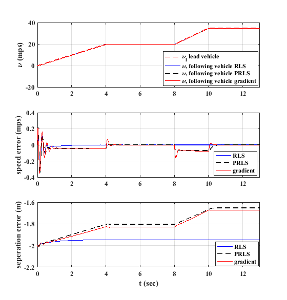
Figure 2: ACC comparison results, speed tracking and separation error in Matlab/Simulink.

$$\dot{\hat{\theta}} =Pr\{\phi P_{ii}e\},$$ (55)

$$\dot{P} =\beta P-P\phi\phi^{T}P,\quad$$

with

$$e=v-v_{m},$$ (56)

$$\theta=\begin{bmatrix}k_{1},&k_{2},&k_{3}\end{bmatrix}^{T},$$

$$\phi=\begin{bmatrix}\frac{v_{r}}{s+a_{m}},&\frac{\delta}{s+a_{m}},&\frac{1}{s+a_{m}}\end{bmatrix}^{T},$$

where $P_{ii}$ are the diagonal elements of $P$ covariance matrix, i=1,2,3.

For gradient based adaptive law, $\gamma_{1}=50,\gamma_{2}=30,\gamma_{3}=40$ constant gains are given. For RLS based algorithm $\beta=0.95$ and $P(0)=100I_{3}$ are given. For both RLS and gradient schemes, a Gaussian noise is applied ($\sigma=0.05$). Simulation results from Matlab/Simulink for throttle system are given in Fig. 2. Fig. 2 shows the vehicle following for both gradient based adaptive law and RLS based adaptive law. The speed error in velocity tracking shows the better performance for RLS adaptive law. Furthermore, it can be inferred from this figure that the RLS provides exponential convergence.

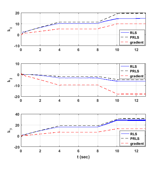
Figure 3: ACC adaptive parameters in Matlab/Simulink.

The adaptive parameters are illustrated in Fig. 3. It is shown that these parameters are achieved adaptively based on the system specifications and they are all stable.

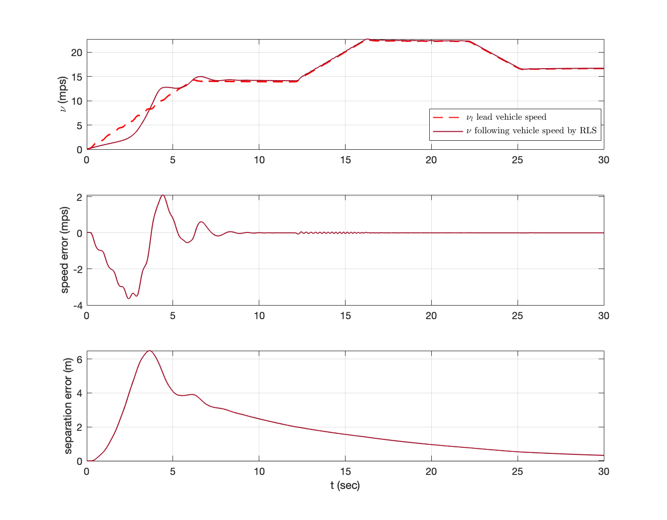
Figure 4: RLS based ACC results in CarSim.

We also implemented RLS based adaptive control algorithm in (55) to CarSim for more realistic results. The vehicle parameters used in CarSim are as follows: $m=567.75\leavevmode\nobreak\ kg$, $R=0.3\leavevmode\nobreak\ m$, $I=1.7\leavevmode\nobreak\ kgm^{2}$, $B=0.01\leavevmode\nobreak\ kg/s$. The adaptive gains for both gradient and RLS are used the same as in Matlab/Simulink. CarSim results for RLS based ACC can be found in Fig. 4. Results demonstrate the ability of the following vehicle equipped with RLS based adaptive law on dry road by adjusting the speed and the distance between the leading vehicle and itself.

V CONCLUSIONS

In this paper, a constructive Lyapunov analysis of RLS based parameter estimation direct adaptive control is proposed. A systematic representation of designing a time varying adaptive gain (covariance) matrix is proposed via Lyapunov analysis, where it is analytically demonstrated that the adaptive parameters converge to the actual ones exponentially fast. The simulation results on an ACC model via Matlab/Simulink, and the comparative achievements, with respect to gradient based method and pure-LS procedure, validate the analytical gains. Moreover, it is shown that LS-based approach outperforms the others. Furthermore, a realistic vehicle software, CarSim, is utilized to scrutinize the applicability of the proposed method on a real ACC system.

References

- [1] P. Ioannou and J. Sun, Robust Adaptive Control. Saddle River, NJ: Prentice-Hall, 1996.
- [2] P. Ioannou and B. Fidan, Adaptive Control Tutorial. Philadelphia, PA: SIAM, 2006.
- [3] K. Narendra and A. Annaswamy, Stable adaptive systems, 2012.
- [4] G. Goodwin and K. Sin, Adaptive filtering prediction and control, 2014.
- [5] M. Krstic, P. Kokotovic, and I. Kanellakopoulos, Nonlinear and adaptive control design, 1995.
- [6] B. Fidan, A. Camlica, and S. Guler, “Least-squares-based adaptive target localization by mobile distance measurement sensors,” International Journal of Adaptive Control and Signal Processing, vol. 29, no. 2, pp. 259–271, 2015.
- [7] S. Guler, B. Fidan, S. Dasgupta, B. D. Anderson, and I. Shames, “Adaptive source localization based station keeping of autonomous vehicles,” IEEE Transactions on Automatic Control, vol. 62, no. 7, pp. 3122–3135, 2016.
- [8] M. Krstic, “On using least-squares updates without regressor filtering in identification and adaptive control of nonlinear systems,” Automatica, vol. 45, p. 731–735, March 2009.
- [9] P. R. Kumar, “Convergence of adaptive control schemes using least-squares parameter estimates,” IEEE Transactions on Automatic Control, vol. 35, no. 4, pp. 416–424, 1990.
- [10] A. Mohanty and B. Yao, “Integrated direct/indirect adaptive robust control of hydraulic manipulators with valve deadband,” IEEE/ASME Transactions on Mechatronics, vol. 16, no. 4, pp. 707–715, 2011.
- [11] J.-J. E. Slotine and W. Li, “Composite adaptive control of robot manipulators,” Automatica, vol. 25, no. 4, pp. 509–519, 1989. [Online]. Available: https://www.sciencedirect.com/science/article/pii/0005109889900940
- [12] N. Koksal, H. An, and B. Fidan, “Backstepping-based adaptive control of a quadrotor uav with guaranteed tracking performance,” ISA Transactions, vol. 105, pp. 98–110, 2020. [Online]. Available: https://www.sciencedirect.com/science/article/pii/S0019057820302524
- [13] P. De Larminat, “On the stabilizability condition in indirect adaptive control,” Automatica, vol. 20, no. 6, pp. 793–795, 1984.
- [14] B. Yao, “Integrated direct/indirect adaptive robust control of siso nonlinear systems in semi-strict feedback form,” in American Control Conference, vol. 4, 2003, pp. 3020–3025.
- [15] C. Hu, B. Yao, and Q. Wang, “Integrated direct/indirect adaptive robust contouring control of a biaxial gantry with accurate parameter estimations,” Automatica, vol. 46, no. 4, pp. 701–707, 2010.
- [16] J. Sternby, “On consistency for the method of least squares using martingale theory,” IEEE Transactions on Automatic Control, vol. 22, no. 3, pp. 346–352, 1977.
- [17] T. Tay, J. Moore, and R. Horowitz, “Indirect adaptive techniques for fixed controller performance enhancement,” International Journal of Control, vol. 50, no. 5, pp. 1941–1959, 1989.
- [18] B. Yao, “High performance adaptive robust control of nonlinear systems: a general framework and new schemes,” in IEEE Conference on Decision and Control, vol. 3, 1997, pp. 2489–2494.
- [19] G. Chowdhary and E. Johnson, “Recursively updated least squares based modification term for adaptive control,” in American Control Conference, 2010, pp. 892–897.
- [20] I. Karafyllis and M. Krstic, “Adaptive certainty-equivalence control with regulation-triggered finite-time least-squares identification,” IEEE Transactions on Automatic Control, vol. 63, no. 10, pp. 3261–3275, 2018.
- [21] K. Jiang and A. Victorino, A.C.and Charara, “Adaptive estimation of vehicle dynamics through rls and kalman filter approaches,” in IEEE 18th International Conference on Intelligent Transportation Systems, 2015, pp. 1741–1746.
- [22] A. Mohanty and B. Yao, “Indirect adaptive robust control of hydraulic manipulators with accurate parameter estimates,” IEEE Transactions on Control Systems Technology, vol. 19, no. 3, pp. 567–575, 2011.
- [23] B. Yao, “High performance adaptive robust control of nonlinear systems: a general framework and new schemes,” in IEEE Conference on Decision and Control, vol. 3, 1997, pp. 2489–2494.
- [24] Y. Ameho, F. Niel, F. Defay, J. Biannic, and C. Berard, “Adaptive control for quadrotors,” in ICRA Robotics and Automation, 2013, pp. 5396–5401.
- [25] R. Leishman, J. Macdonald, R. Beard, and T. McLain, “Quadrotors and accelerometers: State estimation with an improved dynamic model,” IEEE Control Systems, vol. 34, no. 1, pp. 28–41, 2014.
- [26] A. Vahidi, A. Stefanopoulou, and H. Peng, “Recursive least squares with forgetting for online estimation of vehicle mass and road grade: theory and experiments,” Vehicle System Dynamics, vol. 43, no. 1, pp. 31–55, 2005.
- [27] H. Bae, J. Ryu, and J. C. Gerdes, “Road grade and vehicle parameter estimation for longitudinal control using gps,” in Proceedings of the IEEE Conference on Intelligent Transportation Systems, 2001, pp. 25–29.
- [28] D. Pavkovic, J. Deur, G. Burgio, and D. Hrovat, “Estimation of tire static curve gradient and related model-based traction control application,” in IEEE Control Applications,(CCA) & Intelligent Control,(ISIC), 2009, pp. 594–599.
- [29] C. Acosta-Lú, S. D. Gennaro, and M. Sánchez-Morales, “An adaptive controller applied to an anti-lock braking system laboratory,” Dyna, vol. 83, no. 199, pp. 69–77, 2016.
- [30] W. Chen, D. Tan, and L. Zhao, “Vehicle sideslip angle and road friction estimation using online gradient descent algorithm,” IEEE Transactions on Vehicular Technology, vol. 67, no. 12, pp. 11 475–11 485, 2018.
- [31] S. Seyedtabaii and A. Velayati, “Adaptive optimal slip ratio estimator for effective braking on a non-uniform condition road,” Automatika, Journal for Control, Measurement, Electronics, Computing and Communications, vol. 60, no. 4, pp. 413–421, 2019.
- [32] N. Patra and S. Sadhu, “Adaptive extended kalman filter for the state estimation of anti-lock braking system,” in Annual IEEE India Conference (INDICON). IEEE, 2015, pp. 1–6.
- [33] R. Ortega, V. Nikiforov, and D. Gerasimov, “On modified parameter estimators for identification and adaptive control. a unified framework and some new schemes,” Annual Reviews in Control, vol. 50, pp. 278–293, 2020. [Online]. Available: https://www.sciencedirect.com/science/article/pii/S136757882030050X
- [34] A. Goel, A. L. Bruce, and D. S. Bernstein, “Recursive least squares with variable-direction forgetting: Compensating for the loss of persistency [lecture notes],” IEEE Control Systems Magazine, vol. 40, no. 4, pp. 80–102, 2020.