Non-symmetric isogeometric FEM-BEM couplings

Abstract.

We present a coupling of the Finite Element and the Boundary Element Method in an isogeometric framework to approximate either two-dimensional Laplace interface problems or boundary value problems consisting in two disjoint domains. We consider the Finite Element Method in the bounded domains to simulate possibly non-linear materials. The Boundary Element Method is applied in unbounded or thin domains where the material behavior is linear. The isogeometric framework allows to combine different design and analysis tools: first, we consider the same type of NURBS parameterizations for an exact geometry representation and second, we use the numerical analysis for the Galerkin approximation. Moreover, it facilitates to perform $h$- and $p$-refinements. For the sake of analysis, we consider the framework of strongly monotone and Lipschitz continuous operators to ensure well-posedness of the coupled system. Furthermore, we provide an a priori error estimate. We additionally show an improved convergence behavior for the errors in functionals of the solution that may double the rate under certain assumptions. Numerical examples conclude the work which illustrate the theoretical results.

Keywords. Finite Element Method, Boundary Element Method, non-symmetric coupling, Isogeometric Analysis, non-linear operators, Laplacian interface problem, Boundary Value Problems, multiple domains, well-posedness, a priori estimate, super-convergence, electromagnetics, electric machines

Mathematics Subject Classification. 65N12, 65N30, 65N38, 78M10, 78M15

1. Introduction and preliminaries

In the last decades, simulation gained more and more importance as a forth pillar of sciences besides theory, experiments, and observations. A successful simulation means a good imitation of some phenomena. This allows the analysis, optimization, and predictions to be made ad-hoc with a certain reliability, which depends on the application. For example, this can be achieved for problems that are formulated as boundary and initial value problems by choosing the right mathematical model, a good representation of the computational domain, and a suitable numerical method.
We encounter in this work two types of model problems. First, we consider a Laplacian interface problem in Section 2. Its specificity lies in the combination of a possibly non-linear and non-homogeneous problem in a bounded domain with a linear and homogeneous problem in an unbounded domain. This type of model describes a wide class of engineering and physical applications. One example for electromagnetic scattering problems and elastostatics can be found in [Ste11]. We address the second type of model in Section 4. It is a Boundary Value Problem (BVP) with two disjoint domains, which are separated by a (thin) gap. In the domains we allow non-linear equations. However, the gap is assumed to be filled with a linear material, where the simplest form is air. For a visualization we refer to Figure 1. This model is particularly used for the simulation of electro-mechanical energy converters. An example is an electric machine discussed in [BCSDG17]. In general, the air gap is very thin. The other two domains are modeled separately for a facilitation of a possible rotation of the interior part, called rotor in case of an electric machine. This movement is induced by the interaction of electromagnetic fields in the air gap. The computation of forces and torques are therefore one central goal in this type of simulations. Formally, this can be achieved by using the so called Maxwell Stress Tensor (MST) method, see, e.g., [KFK⁺97]. For this, the solution in the air gap as well as its derivatives are needed. These aspects have to be kept in mind for a suitable choice of a numerical method.
The coupling of the Finite Element Method (FEM) and the Boundary Element Methods (BEM) appears to be an intuitive and straightforward choice for the above described problems. Indeed, the FEM is well established and widely used for possibly non-linear problems in bounded domains. On the other side the BEM relies on the transfer of the model problem to an integral representation. Further steps then lead to a Galerkin discretization problem on its boundary with certain integral operators. In a post-processing step, a solution can be found in every point of the underlying domain. Hence, BEM is suitable to handle problems with an unbounded domain where we do not have to truncate the domain since the discretization itself is done on the boundary. We remark that a truncation would be mandatory if we would apply FEM. Since the BEM discretization takes place on a boundary of the domain, it is also very attractive to get a solution in the thin gap described above. For a mesh-based method in the whole domain, e.g., like FEM, it is very difficult to find a mesh for such a thin gap, where the numerical method remains stable. The discretization on the boundary with BEM and the post-processing afterwards avoids this problem. However, to apply the BEM we need to know the fundamental solution of the underlying problem. Note that this restricts the application of BEM especially for non-linear problems. Therefore, we apply BEM in this work for two different applications: first in the exterior unbounded domain and second in the thin air gap. In both cases we consider the Laplace operator for the BEM part, where the fundamental solution can be given explicitly.

In the literature, we distinguish several types of FEM-BEM coupling techniques. These coupling procedures differ solely in the considered representation of the Boundary Integral Equations (BIE), which are the basis for BEM. In order to introduce briefly the considered BIEs, we envisage first the following Laplace equation

(1) $$-\Delta u=0\quad\text{in }\Omega^{\kappa},\quad\kappa=0,1,$$

where $\Omega^{0}\subseteq{\mathbb{R}}^{2}$ is a bounded domain with Lipschitz boundary $\Gamma$, and $\Omega^{1}={\mathbb{R}}^{2}\backslash\overline{\Omega^{0}}$ is the corresponding unbounded domain. Hence, $\Gamma=\overline{\Omega^{0}}\cap\overline{\Omega^{1}}$. Note that (1) is an interior problem for $\kappa=0$ and an exterior problem for $\kappa=1$. In the latter case, we additionally assume the radiation condition $u(x)=C_{\infty}\log|x|+\mathcal{O}(1/|x|)$ for $|x|\to\infty$ with the unknown constant $C_{\infty}$, see also Remark 2.1. For some $x\in\Omega^{\kappa}$, the solution $u(x)$ is given by the representation formula

(2) $$u(x)=(-1)^{\kappa}\left(\int_{\Gamma}G(x,y)\phi(y){\,\operatorname{d}}\sigma_{y}-\int_{\Gamma}\partial_{\nu(y)}G(x,y)u_{|\Gamma}(y){\,\operatorname{d}}\sigma_{y}\right),$$

where $G(x,y)=-\frac{1}{2\pi}\log{|x-y|}$ denotes the fundamental solution of the Laplace operator, $\nu(y)$ is an outer normal vector on $\Gamma$ pointing outward with respect to $\Omega^{0}$ at $y\in\Gamma$, and $\left(u_{|\Gamma},\phi:=\partial_{\nu}u_{|\Gamma}\right)$ are the unknown or partially unknown Cauchy data. Hereby, the notation $u_{|\Gamma}$ means the trace of $u$ with respect to $\Gamma$. Note that we omit to write the trace operators in this work due to readability. Taking the trace of the representation formula yield to the following BIEs, see, e.g., [Ste07, Chapter 7] for more details,

(3) $$u_{|\Gamma}=(-1)^{\kappa}\left(\left(\frac{(-1)^{\kappa}}{2}-\mathcal{K}\right)u_{|\Gamma}+\mathcal{V}\phi\right).$$

The invoked Boundary Integral Operators (BIO), the single layer operator $\mathcal{V}$ and the double layer operator $\mathcal{K}$, are given for smooth enough inputs by

(4) $$(\mathcal{V}\phi)(x)=\int_{\Gamma}G(x,y)\phi(y){\,\operatorname{d}}\sigma_{y},\quad(\mathcal{K}u_{|\Gamma})(x)=\int_{\Gamma}\partial_{\nu(y)}G(x,y)u_{|\Gamma}(y){\,\operatorname{d}}\sigma_{y},$$

and can be extended continuously to linear and bounded operators such that

$$\mathcal{V}:\,H^{s-\frac{1}{2}}(\Gamma)\rightarrow H^{s+\frac{1}{2}}(\Gamma),\quad\mathcal{K}:H^{s+\frac{1}{2}}(\Gamma)\rightarrow H^{s+\frac{1}{2}}(\Gamma),$$

for $s\in[-\frac{1}{2},\frac{1}{2}]$, c.f. [Cos88a, Theorem 1]. In particular, the boundary integral operator $\mathcal{V}$ is additionally symmetric, and ${H^{-\frac{1}{2}}(\Gamma)}$-elliptic, if $\operatorname{diam}\left(\Omega\right)<1$, see, e.g., [Ste07, Theorem 6.23]. The properties of $\mathcal{V}$ induce the norm equivalence

(5) $${\left\lVert\psi\right\rVert}^{2}_{\mathcal{V}}:={\left\langle\psi,\,\mathcal{V}\psi\right\rangle}\simeq{\left\lVert\psi\right\rVert}^{2}_{H^{-\frac{1}{2}}(\Gamma)}.$$

In the previous lines, the mentioned spaces have to be understood as follows: for $k>0$, $H^{k}(\cdot)$ denotes the standard Sobolev space equipped with the usual norm $\|\cdot\|_{H^{k}(\cdot)}$. Moreover, the space $H^{k-\frac{1}{2}}(\Gamma)$ is the trace space of $H^{k}(\Omega)$, and spaces with negative exponents $H^{-k}(\Gamma)$ are defined as dual spaces of $H^{k}(\cdot)$ using the natural duality pairing $\left\langle\cdot,\cdot\right\rangle_{\Gamma}$, which is obtained by the extended $L^{2}$-scalar product $\left(\cdot,\cdot\right)_{\Gamma}$. Furthermore, for the unbounded domain $\Omega^{1}$ we need functions with local behavior and denote them by $H_{\mathrm{loc}}^{1}(\Omega^{1}):=\{v:\Omega^{1}\to\mathbb{R}\big{|}\,v_{|K}\in H^{1}(K)\text{ for all }K\subset\overline{\Omega^{1}}\text{ compact}\}$. Finally, we write ${H^{1}(\Omega)}^{\prime}$ for the dual space of $H^{1}(\Omega)$. We recall that

(6) $${\left\langle\psi,v_{|\Gamma}\right\rangle}_{\Gamma}\leq\|\psi\|_{H^{-\frac{1}{2}}(\Gamma)}\|v_{|\Gamma}\|_{H^{\frac{1}{2}}(\Gamma)}\leq C_{\mathrm{tr}}\|\psi\|_{H^{-\frac{1}{2}}(\Gamma)}\|v\|_{H^{1}(\Omega)},$$

holds for all $v\in H^{1}(\Omega)$ and $\psi\in{H^{-\frac{1}{2}}(\Gamma)}$, where the trace inequality is encoded with the trace constant $C_{\mathrm{tr}}>0$. For some bounded domain $\Omega$, $\left(\cdot,\cdot\right)_{\Omega}$ denotes equivalently the standard $L^{2}$-scalar product in $\Omega$.

In the following, we describe a variational ansatz to get a weak form of the model problem. As mentioned above, there are several coupling strategies possible. If we describe the FEM part by the weak form of the well-known Green’s first formula, a coupling with the weak form of (3) ($\kappa=1$) leads to the so called Johnson-Nédélec coupling introduced in [JN80]. The combined weak form is non-symmetric even though the model problem itself is symmetric. Also a Galerkin discretization leads to a non-symmetric system of linear equations. Therefore, this coupling is also known as non-symmetric coupling, where the unknowns are the $u$ of the FEM part and the conormal derivate $\phi$ of the BEM part. To symmetrize this system in case of a symmetric model problem, we first observe that taking the conormal derivative of (2) leads to another integral equation with two other integral operators. A modification of the Johnson-Nédélec coupling with this additional integral equation renders the coupled problem symmetric. This procedure appeared first in [Cos88b] and is known as Costabel’s symmetric coupling. The price of the symmetry is the use of four BIOs, which is computationally more expensive. However, there are still only two unknowns involved. A coupling method with three unknowns, i.e., additionally the trace $u_{|\Gamma}$ of the BEM part is an unknown, is called a three field coupling [Era12]. A coupling procedure with the so called indirect ansatz is also possible and is called Bielak-MacCamy coupling [BM83]. With this strategy, however, one unknown of the BEM part has no physical meaning.
Because of the advantages of the non-symmetric coupling, we consider in this work only this type of coupling. We will introduce it formally in Section 2. For a long time a mathematical analysis for this coupling was only available for smooth boundaries due to the use of a compactness argument of the double layer operator $\mathcal{K}$; [JN80]. In particular, Lipschitz boundaries were excluded . However, a decade ago Sayas [Say09] provided in fact the first analysis also for Lipschitz boundaries. This work influenced several variations and improvements, e.g., [Ste11, AFF⁺13, EOS17] to mention a few but not all. Hence, the non-symmetric coupling became a more natural choice, especially, if a part of the model problem is non-symmetric or non-linear. In this work, we use the results of [AFF⁺13], where an extension to non-linear interface problems has been addressed and combine this result with the proof shown in [EOS17]. Furthermore, we also use [OS14], which extended the proofs for the linear interface problem to certain Boundary Value Problems, i.e, to the second type of problem considered here. For the linear interface problem with a general second order problem in the interior domain, we also refer to [EOS17] for a rigorous and, to the authors knowledge, sharpest ellipticity estimate. Recently, a complete analysis of a parabolic-elliptic interface problem with a full discretization in the sense of a non-symmetric FEM-BEM coupling for spatial discretization was published in [EES18]. Note that such a system arises, for instance, in the modeling of eddy currents in the magneto-quasi-static regime [MS87].

Now, having described the weak form of the model problem with the proposed FEM and BEM parts, we still need to take two major decisions for a successful simulation: a suitable discretization technique, i.e., choosing concrete ansatz spaces for the FEM and BEM, and a good representation of the geometry. These steps are typically made independently, which complicates meshing and remeshing procedures without altering the original geometry. In order to circumvent this, design step and numerical analysis can be combined by considering the same type of basis functions. Hence the geometrical modeling is also used to design ansatz functions in the Galerkin discretization schemes for the approximation of the solution. Such a method is proposed in [HCB05, CHB09]. It is based on using Non-Uniform Rational B-Splines (NURBS) for the unification of Computer Aided Design (CAD) and Finite Element Analysis (FEA). This method is called IsoGeometric Analysis (IGA). The first isogeometric BEM simulation of collocation type can be found in [PGK⁺09, SSE⁺13]. Moreover, fast methods for isogeometric BEM have been successfully implemented in [HR09, MZBF15, DKSW19], which reduces the known high computational complexity of such an application due to the dense matrices produced by the BEM. This makes the method more attractive even for more realistic and complex applications, see, e.g., [CdFDGS16] and [BCSDG17]. A rigorous mathematical analysis for isogemetric FEM started in [BBadVC⁺06, BadVBSV14] and for isogemetric Galerkin BEM in [Gan14, FGP15, FGHP16, Gan17, FGPS19]. For our purpose the results [BadVBSV14, BDK⁺20] together with [AFF⁺13, EOS17, OS14] play a central role in proving the validity and an a priori error estimate of the FEM-BEM coupling in the isogeometric context, which is done in this manuscript for the first time.
The rest of this paper is organized as follows: in Section 2, the non-linear interface problem is addressed. We consider the framework of Lipschitz continuous and strongly monotone operators such as given in [Zei86] and used in [AFF⁺13]. Strong monotonicity of the non-symmetric weak form is showed equivalently to [EOS17] by adapting the setting to non-linear operators. Moreover, well-posedness of the coupling is stated. Section 3 is devoted to the Galerkin discretization of the non-symmetric coupling. Thereby, we introduce the isogeometric framework and the necessary discrete spaces. We derive some error estimates for the conforming isogeometric discretization. In Section 4, we extend the model to a Boundary Value Problem. More precisely, the model domain is split in two disjoint domains, which are separated by a thin (air) gap. First, a variational formulation of the coupled problem is derived. Then we show well-posedness and stability of the method. Furthermore, we discuss a super-convergence result for the evaluation of the solution in the BEM domain. In the last Section 5, we confirm the theoretical results by conducting one numerical example for each model problem. The work is completed by some conclusions and an outlook.

2. Interface problem

Let $\Omega\subset\mathbb{R}^{2}$ be a bounded domain with Lipschitz boundary $\Gamma=\partial\Omega$ and $\Omega^{\mathrm{e}}:={\mathbb{R}}^{2}\backslash\overline{\Omega}$ the corresponding unbounded (exterior) domain. Furthermore, to guarantee the ${H^{-\frac{1}{2}}(\Gamma)}$-ellipticity of the boundary integral operator $\mathcal{V}$, we assume $\operatorname{diam}\left(\Omega\right)<1$. This assumption can merely be achieved by scaling. We consider the following interface problem: Find $(u,u^{\mathrm{e}})\in H^{1}(\Omega)\times H_{\mathrm{loc}}^{1}(\Omega^{\mathrm{e}})$ such that

(7a) $$-\operatorname{div}\left(\mathcal{U}\nabla u\right) =f \text{in }\Omega,$$

(7b) $$-\Delta u^{\mathrm{e}} =0 \text{in }\Omega^{\mathrm{e}},$$

(7c) $${u}_{|\Gamma}-{u^{\mathrm{e}}}_{|\Gamma} =u_{0} \text{on }\Gamma,$$

(7d) $$\mathcal{U}{\nabla u}_{|\Gamma}\cdot\nu-{\nabla u^{\mathrm{e}}}_{|\Gamma}\cdot\nu =\phi_{0} \text{on }\Gamma,$$

(7e) $$u^{\mathrm{e}} =\mathcal{O}\left(|x|^{-1}\right) \text{for }|x|\rightarrow\infty.$$

We remind that $\nu$ denotes the outer normal vector with respect to $\Omega$ and $\mathcal{U}:\,{\mathbb{R}}^{2}\rightarrow{\mathbb{R}}^{2}$ is a possibly non-linear diffusion tensor. The right-hand side is given by $f\in{H^{1}(\Omega)}^{\prime}$, $u_{0}\in{H^{\frac{1}{2}}(\Gamma)}$ is the jump in the Dirichlet data, and $\phi_{0}\in{H^{-\frac{1}{2}}(\Gamma)}$ the jump in the Neumann data.
To ensure the right radiation condition (7e) at infinity, we have to assume the additional condition

$${\left\langle{\nabla u^{\mathrm{e}}}_{|\Gamma}\cdot\nu,1\right\rangle}_{\Gamma}=0.$$

This can be transformed into a compatibility condition on the data, i.e.,

$$\left(f,1\right)_{\Omega}+{\left\langle\phi_{0},1\right\rangle}_{\Gamma}=0.$$

Remark 2.1.

Note that the assumption to ensure the radiation condition is only needed in the two dimensional case. Alternatively, (7e) can be replaced by a logarithmic decay of the solution in two dimensions to avoid the additional assumption on ${\nabla u^{\mathrm{e}}}_{|\Gamma}$, i.e.,

$$u^{\mathrm{e}}=C\log|x|+\mathcal{O}\left(|x|^{-1}\right),\quad\text{ for }|x|\rightarrow\infty,$$

with $C:=\frac{1}{2\pi}{\left\langle{\nabla u^{\mathrm{e}}}_{|\Gamma}\cdot\nu,1\right\rangle}_{\Gamma}$ or equivalently $C:=-\frac{1}{2\pi}\left(\left(f,1\right)_{\Omega}+{\left\langle\phi_{0},1\right\rangle}_{\Gamma}\right)$, which can be easily verified in the weak formulation below.

As mentioned above, the diffusion tensor $\mathcal{U}$ can be a non-linear operator. To apply standard theory for non-linear operators, see, e.g., [Zei86], we assume throughout the manuscript that $\mathcal{U}$ is Lipschitz continuous and strongly monotone:

1. Lipschitz continuity:

   $$\exists\,C^{\mathcal{U}}_{\mathrm{Lip}}>0\text{ such that }|\mathcal{U}x-\mathcal{U}y|\leq C^{\mathcal{U}}_{\mathrm{Lip}}\,|x-y|,\,\forall x,y\in{\mathbb{R}}^{2}.$$

2. strong monotonicity:

   $$\exists\,C^{\mathcal{U}}_{\mathrm{ell}}>0\text{ such that }\left(\mathcal{U}\nabla u-\mathcal{U}\nabla v,\nabla u-\nabla v\right)_{\Omega}\geq C^{\mathcal{U}}_{\mathrm{ell}}\,{\left\lVert\nabla u-\nabla v\right\rVert}^{2}_{L^{2}(\Omega)},\,\forall u,v\in{H^{1}(\Omega)}.$$

The derivation of a non-symmetric variational form follows a standard procedure: In the variational form of (7a), we replace the Neumann data by the jump condition (7d) to couple the interior problem with the conormal derivative with $\phi:=\partial_{\nu}u^{\mathrm{e}}_{|\Gamma}=\nabla u^{\mathrm{e}}_{|\Gamma}\cdot\nu$ of the exterior problem. For the second equation we use the exterior integral equation (3) with $\kappa=1$, and insert the jump condition (7c) to couple this with the interior trace.
Hence, the weak formulation of the non-symmetric coupling problem reads: Find $\mathbf{u}=(u,\phi)\in H^{1}(\Omega)\times{H^{-\frac{1}{2}}(\Gamma)}$ such that

$$\left(\mathcal{U}\nabla u,\nabla v\right)_{\Omega}-\left\langle\phi,v_{|\Gamma}\right\rangle_{\Gamma} =\left(f,v\right)_{\Omega}+\left\langle\phi_{0},v_{|\Gamma}\right\rangle_{\Gamma},$$

$$\left\langle\psi,\left(\frac{1}{2}-\mathcal{K}\right)u_{|\Gamma}\right\rangle_{\Gamma}+\left\langle\psi,\mathcal{V}\phi\right\rangle_{\Gamma} =\left\langle\psi\left(\frac{1}{2}-\mathcal{K}\right)u_{0}\right\rangle_{\Gamma}$$

holds $\forall\mathbf{v}=\left(v,\psi\right)\in H^{1}(\Omega)\times{H^{-\frac{1}{2}}(\Gamma)}$.
This variational form can be written in a compact form. For this we introduce a product space with corresponding norm, i.e.,

(8) $$\mathcal{H}:=H^{1}(\Omega)\times{H^{-\frac{1}{2}}(\Gamma)},\qquad{\left\lVert\mathbf{v}\right\rVert}_{\mathcal{H}}:=\big{(}{\left\lVert v\right\rVert}_{H^{1}(\Omega)}^{2}+{\left\lVert\psi\right\rVert}_{{H^{-\frac{1}{2}}(\Gamma)}}^{2}\big{)}^{\frac{1}{2}}\text{ for }\mathbf{v}=(v,\psi)\in\mathcal{H}.$$

Problem 2.2.

Find $\mathbf{u}\in\mathcal{H}:=H^{1}(\Omega)\times{H^{-\frac{1}{2}}(\Gamma)}$ such that $a(\mathbf{u},\mathbf{v})=\ell(\mathbf{v})$ holds $\forall\mathbf{v}\in\mathcal{H}$ with the linear form (linear in the second argument) $a:\mathcal{H}\times\mathcal{H}\to\mathbb{R}$,

(9) $$a(\mathbf{u},\mathbf{v}):=\left(\mathcal{U}\nabla u,\nabla v\right)_{\Omega}-{\left\langle\phi,v_{|\Gamma}\right\rangle}_{\Gamma}+{\left\langle\psi,\left(\frac{1}{2}-\mathcal{K}\right)u_{|\Gamma}\right\rangle}_{\Gamma}+{\left\langle\psi,\mathcal{V}\phi\right\rangle}_{\Gamma},$$

and the linear functional $\ell$ on $\mathcal{H}$,

(10) $$\ell(\mathbf{v}):=\left(f,v\right)_{\Omega}+\left\langle\phi_{0},v_{|\Gamma}\right\rangle_{\Gamma}+\left\langle\psi,\left(\frac{1}{2}-\mathcal{K}\right)u_{0}\right\rangle_{\Gamma}.$$

It is easy to check that $a(\mathbf{v},\mathbf{v})$ is not elliptic, e.g., insert $\mathbf{v}=(1,0)$. Hence, [AFF⁺13] suggested an implicit stabilization where the stabilized problem is equivalent to the original one, i.e., a solution of the original problem is also a solution of the stabilized one and vice versa. Thus, the analysis is done with the aid of the stabilized form, i.e., well-posedness is inherited to the original problem. For implementation purposes, we still use the original problem. The stabilized problem reads:

Problem 2.3.

Find $\mathbf{u}\in\mathcal{H}$ such that $\widetilde{a}(\mathbf{u},\mathbf{v})=\widetilde{\ell}(\mathbf{v})$ holds $\forall\mathbf{v}\in\mathcal{H}$, where we define with

$$s(\mathbf{v}):={\left\langle 1,\left(\frac{1}{2}-\mathcal{K}\right)v_{|\Gamma}\right\rangle}_{\Gamma}+{\left\langle 1,\mathcal{V}\psi\right\rangle}_{\Gamma},\qquad\mathbf{v}=(v,\psi)$$

the stabilized linear form

$$\widetilde{a}(\mathbf{u},\mathbf{v}):=a(\mathbf{u},\mathbf{v})+s(\mathbf{u})s(\mathbf{v}),$$

and the functional

$$\widetilde{\ell}(\mathbf{v}):=\ell(\mathbf{v})+{\left\langle 1,\left(\frac{1}{2}-\mathcal{K}\right)u_{0}\right\rangle}_{\Gamma}s(\mathbf{v}).$$

Lemma 2.4 ([AFF⁺13]).

The original and the stabilized formulation are equivalent, i.e., $\mathbf{u}\in\mathcal{H}$ solves Problem 2.2 if and only if it solves Problem 2.3, and vice versa.

In order to state well-posedness for Problem 2.3, and thanks to Lemma 2.4 also for Problem 2.2, we follow standard results for monotone operatos [Zei86]. First, we note that the form $\widetilde{a}(\mathbf{u},\mathbf{v})$ induces a non-linear operator $\widetilde{\mathcal{A}}:\mathcal{H}\rightarrow\mathcal{H}^{\prime}$ by

(11) $${\left\langle\widetilde{\mathcal{A}}(\mathbf{u}),\mathbf{v}\right\rangle}:=\widetilde{a}(\mathbf{u},\mathbf{v}),\quad\forall\mathbf{u},\mathbf{v}\in\mathcal{H},$$

where $\mathcal{H}^{\prime}$ denotes the dual space of $\mathcal{H}$. This allows us to prove the following lemma.

Lemma 2.5 ([AFF⁺13, EOS17]).

Let us consider the non-linear operator $\widetilde{\mathcal{A}}:\mathcal{H}\rightarrow\mathcal{H}^{\prime}$ defined in (11) with $\mathcal{H}=H^{1}(\Omega)\times{H^{-\frac{1}{2}}(\Gamma)}$. The following assertions hold.

• $\widetilde{\mathcal{A}}$ is Lipschitz continuous, i.e., there exists $C_{\mathrm{Lip}}>0$ such that

  $${\left\lVert\widetilde{\mathcal{A}}(\mathbf{u})-\widetilde{\mathcal{A}}(\mathbf{v})\right\rVert}_{\mathcal{H}^{\prime}}\leq C_{\mathrm{Lip}}{\left\lVert\mathbf{u}-\mathbf{v}\right\rVert}_{\mathcal{H}},$$

  for all $\mathbf{u}$, $\mathbf{v}\in\mathcal{H}$.

• if $C^{\mathcal{U}}_{\mathrm{ell}}>\frac{1}{4}$, there holds that

  (12) $${\left\langle\widetilde{\mathcal{A}}(\mathbf{u})-\widetilde{\mathcal{A}}(\mathbf{v}),\mathbf{u}-\mathbf{v}\right\rangle}\geq C_{\mathrm{stab}}\left({\left\lVert\nabla u-\nabla v\right\rVert}_{L^{2}(\Omega)}^{2}+{\left\lVert\phi-\psi\right\rVert}^{2}_{\mathcal{V}}+s(\mathbf{\mathbf{u}-\mathbf{v}})^{2}\right),$$

  for all $\mathbf{u}=(u,\phi)\in\mathcal{H}$, $\mathbf{v}=(v,\psi)\in\mathcal{H}$ with the norm ${\left\lVert\psi\right\rVert}^{2}_{\mathcal{V}}:={\left\langle\psi,\,\mathcal{V}\psi\right\rangle}$ and with

  $$C_{\mathrm{stab}}=\min\left\{1,\frac{1}{2}\left(1+C^{\mathcal{U}}_{\mathrm{ell}}-\sqrt{\left(C^{\mathcal{U}}_{\mathrm{ell}}-1\right)^{2}+1}\right)\right\}.$$

• if $C^{\mathcal{U}}_{\mathrm{ell}}>\frac{1}{4}$, then $\widetilde{\mathcal{A}}$ is strongly monotone , i.e., there exists $C_{\mathrm{ell}}>0$ such that

  $${\left\langle\widetilde{\mathcal{A}}(\mathbf{u})-\widetilde{\mathcal{A}}(\mathbf{v}),\mathbf{u}-\mathbf{v}\right\rangle}\geq C_{\mathrm{ell}}{\left\lVert\mathbf{u}-\mathbf{v}\right\rVert}^{2}_{\mathcal{H}}$$

  for all $\mathbf{u}$, $\mathbf{v}\in\mathcal{H}$.

Proof.

The Lipschitz continuity of $\widetilde{\mathcal{A}}$ follows from the Lipschitz continuity of $\mathcal{U}$, and the continuity of the integral operators.
The proof of the second assertion follows the lines of [EOS17, Theorem 1] for $\beta=1$. We replace the coercivity estimate of the bilinear form $\left(\mathcal{U}\nabla u,\nabla v\right)_{\Omega}$ considered in [EOS17] for a linear $\mathcal{U}$ by the strong monotonicity property of $\mathcal{U}$, i.e,

$$\left(\mathcal{U}\nabla u-\mathcal{U}\nabla v,\nabla u-\nabla v\right)_{\Omega}\geq C^{\mathcal{U}}_{\mathrm{ell}}\,{\left\lVert\nabla u-\nabla v\right\rVert}^{2}_{L^{2}(\Omega)}.$$

The restriction of $C^{\mathcal{U}}_{\mathrm{ell}}$ is a direct result of the use of a contractivity result for the double layer operator $\mathcal{K}$ [OS13, Lemma 2.1] with a constant $C_{\mathcal{K}}\in[\frac{1}{2},1)$, where we use the worst case of $C_{\mathcal{K}}=1$ in the statement.
For the last assertion we note the norm equivalence (5), and by a a Rellich compactness argument it can be shown [AFF⁺13, Lemma 10] that

$${\left|\kern-1.07639pt\left|\kern-1.07639pt\left|\mathbf{v}\right|\kern-1.07639pt\right|\kern-1.07639pt\right|}^{2}:={\left\lVert\nabla v\right\rVert}_{L^{2}(\Omega)}^{2}+{\left\lVert\psi\right\rVert}^{2}_{\mathcal{V}}+s(\mathbf{v})^{2}$$

defines an equivalent norm in $\mathcal{H}$ for some $\mathbf{v}:=\left(v,\psi\right)\in\mathcal{H}$. This leads together with (12) to the last assertion. ∎

The following theorem follows directly from the theoretical result [Zei86, Theorem 25.B].

Theorem 2.6 (Well-posedness, [Zei86]).

Let $C^{\mathcal{U}}_{\mathrm{ell}}>\frac{1}{4}$. Since the induced operator $\widetilde{\mathcal{A}}$ of $\widetilde{a}(\cdot,\cdot)$ is strongly monotone and Lipschitz continuous, there exists a unique solution $\mathbf{u}:=(u,\phi)\in\mathcal{H}$ of the variational Problem 2.3 for any $(f,u_{0},\phi_{0})\in{H^{1}(\Omega)}^{\prime}\times{H^{\frac{1}{2}}(\Gamma)}\times{H^{-\frac{1}{2}}(\Gamma)}$. Thanks to Lemma 2.4, this is also the unique solution of Problem 2.2.

For some engineering applications, where the non-linear operator $\mathcal{U}$ has a special form, we can state the following stabilization result.

Lemma 2.7.

Let all the assumptions of Theorem 2.6 hold and let the non-linear operator $\mathcal{U}$ be of the form $\mathcal{U}\nabla u:=g(|\nabla u|)\nabla u$ with a non-linear function $g:\mathbb{R}\to\mathbb{R}$. Then, for the solution $\mathbf{u}:=(u,\phi)\in\mathcal{H}$ of Problem 2.2, we have the stability result

$${\left\lVert\mathbf{u}\right\rVert}_{\mathcal{H}}\leq C\left({\left\lVert f\right\rVert}_{{H^{1}(\Omega)}^{\prime}}+{\left\lVert u_{0}\right\rVert}_{H^{\frac{1}{2}}(\Gamma)}+{\left\lVert\phi_{0}\right\rVert}_{H^{-\frac{1}{2}}(\Gamma)}\right),\quad C>0.$$

Proof.

Let $\mathbf{v}\in\mathcal{H}$ be arbitrary. We know from the strong monotonicity of $\widetilde{\mathcal{A}}$ that

$$C_{\mathrm{ell}}{\left\lVert\mathbf{u}-\mathbf{v}\right\rVert}^{2}_{\mathcal{H}}\leq{\left\langle\widetilde{\mathcal{A}}(\mathbf{u})-\widetilde{\mathcal{A}}(\mathbf{v}),\mathbf{u}-\mathbf{v}\right\rangle}.$$

Without loss of generality, we choose $\mathbf{v}=\left(0,0\right)$ and note that $\mathcal{U}\nabla v=0$. Thanks to Lemma 2.4 $\mathbf{u}:=\left(u,\phi\right)$ is also the unique solution of the Problem 2.3. Thus, we conclude that

$$C_{\mathrm{ell}}{\left\lVert\mathbf{u}\right\rVert}^{2}_{\mathcal{H}} \leq{\left\langle\widetilde{\mathcal{A}}(\mathbf{u}),\mathbf{u}\right\rangle}=\widetilde{\ell}(\mathbf{u}),$$

$$=\left(f,u\right)_{\Omega}+\left\langle\phi_{0},u_{|\Gamma}\right\rangle_{\Gamma}+\left\langle\phi,\left(\frac{1}{2}-\mathcal{K}\right)u_{0}\right\rangle_{\Gamma}+{\left\langle 1,\left(\frac{1}{2}-\mathcal{K}\right)u_{0}\right\rangle}_{\Gamma}s(\mathbf{u}),$$

with $s(\mathbf{u}):={\left\langle 1,\left(\frac{1}{2}-\mathcal{K}\right)u_{|\Gamma}\right\rangle}_{\Gamma}+{\left\langle 1,\mathcal{V}\phi\right\rangle}_{\Gamma}$. Next we use inequality (6) along with the boundedness of $\mathcal{K}$ and $\mathcal{V}$. Then, rearranging the terms yield to

$$C_{\mathrm{ell}}{\left\lVert\mathbf{u}\right\rVert}^{2}_{\mathcal{H}} \leq\left({\left\lVert f\right\rVert}_{{H^{1}(\Omega)}^{\prime}}+C_{\mathrm{tr}}{\left\lVert\phi_{0}\right\rVert}_{H^{-\frac{1}{2}}(\Gamma)}+\left(\frac{1}{2}+C^{\mathcal{K}}\right)^{2}C_{\mathrm{tr}}{\left\lVert u_{0}\right\rVert}_{H^{\frac{1}{2}}(\Gamma)}\right){\left\lVert u\right\rVert}_{H^{1}(\Omega)}$$

$$+\left(\left(\frac{1}{2}+C^{\mathcal{K}}\right)\left(1+C^{\mathcal{V}}\right){\left\lVert u_{0}\right\rVert}_{H^{\frac{1}{2}}(\Gamma)}\right){\left\lVert\phi\right\rVert}_{H^{-\frac{1}{2}}(\Gamma)},$$

where $C^{\mathcal{K}},\,C^{\mathcal{V}}>0$ denote the continuity constants of the boundary integral operators $\mathcal{K}$ and $\mathcal{V}$, respectively. From this follows the assertion with a constant $C>0$ that depends on $C^{\mathcal{K}},\,C^{\mathcal{V}},\,C_{\mathrm{tr}}$, $C_{\mathrm{ell}}$ and $\Gamma$. ∎

Remark 2.8.

Because of Lemma 2.4, the results obtained for the stabilized formulation also hold true for the original non-symmetric coupling of Problem 2.2. Hence, in the next section, we only discretize the original problem using a Galerkin approximation. In fact, the stabilized version is only used for analysis purposes.

3. Galerkin discretization

Let $V_{\ell}\subset{H^{1}(\Omega)}$ and $X_{\ell}\subset{H^{-\frac{1}{2}}(\Gamma)}$ be some finite dimensional subspaces, where the index $\ell$ expresses a refinement level, e.g., in a sequence of mesh refinements. We assume that:

1. The discrete space $X_{\ell}$ contains the constants, i.e.,

   $$\exists\xi\in\bigcap_{\ell\in\mathbb{N}_{0}}X_{\ell}\text{ such that }{\left\langle\xi,1\right\rangle}_{\Gamma}\neq 0.$$

We consider a conforming Galerkin discretization of the Problem 2.2. Replacing the spaces ${H^{1}(\Omega)}$ and ${H^{-\frac{1}{2}}(\Gamma)}$ with $V_{\ell}$ and $X_{\ell}$, respectively, yields to the following discrete problem: Find $\mathbf{u}_{\ell}=(u_{\ell},\phi_{\ell})\in\mathcal{H}_{\ell}=V_{\ell}\times X_{\ell}$ such that

$$\left\langle\mathcal{U}\nabla u_{\ell},\nabla v_{\ell}\right\rangle_{\Omega}-\left\langle\phi_{\ell},v_{\ell}\right\rangle_{\Gamma} =\left\langle f,v_{\ell}\right\rangle_{\Omega}+\left\langle\phi_{0},v_{\ell}\right\rangle_{\Gamma},$$

$$\left\langle\psi_{\ell},\left(\frac{1}{2}-\mathcal{K}\right)u_{\ell}\right\rangle_{\Gamma}+\left\langle\psi_{\ell},\mathcal{V}\phi_{\ell}\right\rangle_{\Gamma} =\left\langle\psi_{\ell},\left(\frac{1}{2}-\mathcal{K}\right)u_{0}\right\rangle_{\Gamma}$$

holds $\forall\mathbf{v}_{\ell}=\left(v_{\ell},\psi_{\ell}\right)\in\mathcal{H}_{\ell}$.
The compact form in the product space $\mathcal{H}_{\ell}$ reads:

Problem 3.1.

Find $\mathbf{u}_{\ell}=(u_{\ell},\phi_{\ell})\in\mathcal{H}_{\ell}=V_{\ell}\times X_{\ell}$ such that $a(\mathbf{u}_{\ell},\mathbf{v}_{\ell})=\ell(\mathbf{v}_{\ell})$ holds $\forall\mathbf{v_{\ell}}=(v_{\ell},\psi_{\ell})\in\mathcal{H}_{\ell}$. The linear form $a(\cdot,\cdot)$ and the linear functional $\ell$ are defined in (9) and (10), respectively.

Provided that Assumption (A$3$) is satisfied, the analysis for Problem 3.1 is done analogously to the continuous Problem 2.2 since the discrete spaces are conform. In other words, all the above results including the introduction of a stabilized form and Lemma 2.4 also hold for the subspaces. In particular, due to Theorem 2.6 the discrete solution $\mathbf{u}_{\ell}=(u_{\ell},\phi_{\ell})\in\mathcal{H}_{\ell}=V_{\ell}\times X_{\ell}$ of Problem 3.1 exists and is unique. The following quasi-optimality result in the sense of the Céa-type Lemma is a standard but central result, which will be needed in Subsection 3.2 for the a priori error estimate of the non-symmetric coupling.

Theorem 3.2 (Quasi-optimality).

Let Assumption (A$3$) hold, and $C^{\mathcal{U}}_{\mathrm{ell}}>\frac{1}{4}$. Moreover, let $\mathbf{u}:=\left(u,\phi\right)\in\mathcal{H}$ be the unique solution of Problem 2.2, and $\mathbf{u}_{\ell}:=\left(u_{\ell},\phi_{\ell}\right)\in\mathcal{H}_{\ell}$ the solution of its discrete counterpart Problem 3.1. It holds that

$${\left\lVert u-u_{\ell}\right\rVert}_{H^{1}(\Omega)}+{\left\lVert\phi-\phi_{\ell}\right\rVert}_{H^{-\frac{1}{2}}(\Gamma)}\leq C_{\text{C\'{e}a}}\min_{v_{\ell}\in V_{\ell},\psi_{\ell}\in X_{\ell}}\left({\left\lVert u-v_{\ell}\right\rVert}_{H^{1}(\Omega)}+{\left\lVert\phi-\psi_{\ell}\right\rVert}_{H^{-\frac{1}{2}}(\Gamma)}\right),$$

with $C_{\text{C\'{e}a}}=\frac{C_{\mathrm{Lip}}}{C_{\mathrm{ell}}}$.

Proof.

The assertion follows as a result of the main theorem on strongly monotone operators [Zei86, Corollary 25.7]. That means with $\mathbf{v}_{\ell}=(v_{\ell},\psi_{\ell})$, thanks to Lemma 2.4, the strong monotonicity, Galerkin orthogonality, Cauchy-Schwarz inequality, and the Lipschitz continuity we get

$$C_{\mathrm{ell}}{\left\lVert\mathbf{u}-\mathbf{u}_{\ell}\right\rVert}^{2}_{\mathcal{H}} \leq{\left\langle\widetilde{\mathcal{A}}(\mathbf{u})-\widetilde{\mathcal{A}}(\mathbf{u}_{\ell}),\mathbf{u}-\mathbf{u}_{\ell}\right\rangle}={\left\langle\widetilde{\mathcal{A}}(\mathbf{u})-\widetilde{\mathcal{A}}(\mathbf{u}_{\ell}),\mathbf{u}-\mathbf{v}_{\ell}\right\rangle}\leq{\left\lVert\widetilde{\mathcal{A}}(\mathbf{u})-\widetilde{\mathcal{A}}(\mathbf{u}_{\ell})\right\rVert}_{\mathcal{H}^{\prime}}{\left\lVert\mathbf{u}-\mathbf{v}_{\ell}\right\rVert}_{\mathcal{H}}$$

$$\leq C_{\mathrm{Lip}}{\left\lVert\mathbf{u}-\mathbf{u}_{\ell}\right\rVert}_{\mathcal{H}}{\left\lVert\mathbf{u}-\mathbf{v}_{\ell}\right\rVert}_{\mathcal{H}},$$

where the assertion follows directly. ∎

3.1. Isogeometric Analysis

The basis functions that are considered for the geometry design in the isogeometric framework are used as ansatz functions for the Galerkin discretization. These functions are typically B-Splines or some extensions of B-Splines, e.g., NURBS, T-Splines etc.
In the following, we introduce briefly the concept of Isogeometric Analysis and refer to [CHB09] for a more detailed introduction, and to [BadVBSV14] and [BDK⁺20] for a mathematical analysis of IGA in the FEM and BEM context, respectively.

Definition 3.3.

Let $p\in\mathbb{N}$ denote the degree, and $k\in\mathbb{N}$ the number of the B-Spline basis functions, with $k>p$. A knot vector $\Xi:=\{\xi_{0},\dots,\xi_{k+p}\}$ is called $p$-open if

$$0=\xi_{0}=\dots=\xi_{p}<\xi_{p+1}\leq\dots\leq\xi_{k-1}<\xi_{k}=\dots=\xi_{k+p}=1.$$

Associated to the knot vector $\Xi$, $k$ B-Spline basis functions can be defined recursively for $p\geq 1$ by

$$b_{i}^{p}(x)=\frac{x-\xi_{i}}{\xi_{i+p}-\xi_{i}}b_{i}^{p-1}(x)+\frac{\xi_{i+p+1}-x}{\xi_{i+p+1}-\xi_{i+1}}b_{i+1}^{p-1}(x),$$

for all $i=0\dots k-1$, starting with piecewise constant basis functions for $p=0$, namely,

$$b_{i}^{0}(x)=\begin{cases}1&\text{if }\xi_{i}\leq x\leq\xi_{i+1}\\ 0&\text{otherwise}\end{cases}.$$

Moreover, we denote by $\mathbb{S}_{p}(\Xi)=\operatorname{span}{\{(b_{i}^{p})_{i=0\dots k-1}\}}$ the space of B-Splines of degree $p$ and dimension $k$ in the parameter domain over the knot vector $\Xi$.

Definition 3.4.

Let $f:[0,1]\rightarrow\gamma\subset{\mathbb{R}}^{d}$ be a B-Spline mapping defined as

$$f(x)=\sum_{i=0}^{k-1}c_{i}b_{i}^{p}(x)$$

with $c_{i}\in{\mathbb{R}}^{d}$ representing an element of a set of control points. The mapping $f$ describes a one-dimensional curve embedded in a $d$-dimensional Euclidian space and is called a B-Spline curve. Moreover, we call $\gamma$ a patch if the mapping $f$ is regular.

As long as the B-Spline mapping $f$ is regular, we can define B-Spline spaces in the physical domain, i.e., over a patch $\gamma$ by using the following transformation

$$\iota(f)(u)=u\circ f,$$

namely,

$$\mathbb{S}_{p}(\gamma)=\{v:v=\iota(f)(u)^{-1},u\in\mathbb{S}_{p}(\Xi)\}.$$

Definition 3.5.

B-Spline spaces on higher dimensional domains are constructed by using tensor product relationships. For example, in $2D$, we write with $p_{1},p_{2}\in\mathbb{N}$ and $k_{1},k_{2}\in\mathbb{N}$

$$\mathbb{S}_{p_{1},p_{2}}(\Xi_{1},\Xi_{2})=\operatorname{span}{\{(b_{i_{1}}^{p_{1}})_{i_{1}=0\dots k_{1}-1}\cdot(b_{i_{2}}^{p_{2}})_{i_{2}=0\dots k_{2}-1}\}},$$

where $p_{1}$ and $p_{2}$ denote the degrees in each parametric direction, and $k_{1}k_{2}$ is the number of the B-Splines basis functions. A B-Spline surface is thus represented by $\mathbf{f}(x):[0,1]^{2}\rightarrow\omega\subset{\mathbb{R}}^{d}$ with

$$\mathbf{f}(x)=\sum_{i_{1}=0}^{k_{1}-1}\sum_{i_{2}=0}^{k_{2}-1}\mathbf{c}_{i_{1},i_{2}}\cdot b_{i_{1}}^{p_{1}}(x)\cdot b_{i_{2}}^{p_{2}}(x),$$

and $\mathbf{c}_{i_{1},i_{2}}\in{\mathbb{R}}^{d}$ representing an element of a set of control points. If $f$ is regular, we call $\omega$ a patch.
Equivalently, the two-dimensional B-Spline space in the physical domain is defined over a patch $\omega$ by

$$\mathbb{S}_{p_{1},p_{2}}(\omega)=\{v:v=\iota(\mathbf{f})(u)^{-1},u\in\mathbb{S}_{p_{1},p_{2}}(\Xi_{1},\Xi_{2})\}.$$

Note that for the sake of simplicity, if $p_{1}=p_{2}=p$, a B-Spline space of degree $p$ should be understood as a B-Spline space of degree $p$ in each parametric direction.

The parametrization of curves and surfaces using B-Spline functions allows an exact representation of a large spectrum of geometries. However, they fail to represent conic sections exactly, which are widely present in the design of various engineering applications. In order to circumvent this, Non-Uniform Rational B-Splines (NURBS) are used instead, see [CHB09] and [PT12], for instance.

Definition 3.6.

Let $p,k,p_{1},p_{2},k_{1},k_{2}\in\mathbb{N}$ as above. NURBS mappings can be considered as weighted B-Spline mappings. They can be defined as follows,

$$r(x):=\sum_{i=0}^{k-1}\frac{c_{i}w_{i}b_{i}^{p}(x)}{\sum_{j=0}^{k-1}w_{j}b_{j}^{p}(x)}\quad\text{ in $1$D},$$

$$\mathbf{r}(x):=\sum_{i_{1}=0}^{k_{1}-1}\sum_{i_{2}=0}^{k_{2}-1}\frac{\mathbf{c}_{i_{1},i_{2}}w_{i_{1},i_{2}}\cdot b_{i_{1}}^{p_{1}}(x)\cdot b_{i_{2}}^{p_{2}}(x)}{\sum_{j_{1}=0}^{k_{1}-1}\sum_{j_{2}=0}^{k_{2}-1}w_{j_{1},j_{2}}\cdot b_{j_{1}}^{p_{1}}(x)\cdot b_{j_{2}}^{p_{2}}(x)}\quad\text{ in $2$D.}$$

Thereby, $w_{i},\,w_{i_{1},i_{2}}\in{\mathbb{R}}$ are elements of a vector of dimension $k$ and a matrix of dimension $k_{1}\times k_{2}$, containing weighting coefficients of the NURBS, respectively, and $c_{i},\mathbf{c}_{i_{1},i_{2}}$ are the control points.

Remark 3.7.

Contrary to B-Splines, NURBS spaces on higher dimensional domains cannot be defined using simple tensor product relationships.

In order to guarantee the existence of a regular mapping between the parameter and the physical domain, multiple patches defined through a family of regular parameterizations may in some cases be necessary.

Definition 3.8.

Let $\Omega$ be a two-dimensional Lipschitz domain with boundary $\Gamma$. The domain $\Omega$ is called a multipatch domain, if there exists a family of $N_{\Omega}$ disjoint patches such that $\Omega=\bigcup_{i}\Omega_{i}$ and a regular parametrization $\mathbf{r}_{i}(x):[0,1]^{2}\rightarrow\Omega_{i}$ for every single patch $\Omega_{i}$, with $0\leq i<N_{\Omega}$. Furthermore, we require the parametrization at interfaces to coincide.
Equivalently, $\Gamma$ is also considered a multipatch domain with $\Gamma=\bigcup_{i}\Gamma_{i}$ and $r_{i}(x):[0,1]\rightarrow\Gamma_{i}$, $\forall\Gamma_{i}$, with $0\leq i<N_{\Gamma}$.

Knowing that B-Splines form a partition of unity [PT12], it is easy to see that B-Splines are a special type of NURBS, when the weightings are equal to $1$.

In the following, if we refer to the geometry, we mean NURBS mappings. If we refer to the spaces used for the discretizations, we mean B-Spline mappings. The motivation for this follows from [BDK⁺20], namely, the spline preserving property of B-Splines is needed for a conforming discretization of the De Rham complex.

3.2. Error estimates for an isogeometric FEM-BEM discretization

Let the assumptions of Section 2 on $\Omega$ hold. We consider the discrete Problem 3.1 with $V_{\ell}=\mathbb{S}^{0}(\Omega)$ and $X_{\ell}=\mathbb{S}^{2}(\Gamma)$, where $\mathbb{S}^{0}(\Omega)$ and $\mathbb{S}^{2}(\Gamma)$ are B-Spline spaces defined as in [BDK⁺20] and [BadVBSV14]. Namely,

(13) $$\mathbb{S}^{0}(\Omega)=\{u\in{H^{1}(\Omega)}:u_{|\Omega_{i}}\in\mathbb{S}_{p,p}(\Omega_{i}),\,\forall\,0\leq i<N_{\Omega}\},$$

and

(14) $$\mathbb{S}^{2}(\Gamma)=\{\phi\in{H^{-\frac{1}{2}}(\Gamma)}:\phi_{|\Gamma_{i}}\in\mathbb{S}_{p-1}(\Gamma_{i}),\,\forall\,0\leq i<N_{\Gamma}\}.$$

Thereby, $N_{\Omega}$ and $N_{\Gamma}$ denote the number of domain patches and boundary patches, respectively. Note that the degrees of the B-Spline spaces (13) and (14) are solely fixed by one parameter $p>0$.

Definition 3.9.

Let $\Xi=\{\xi_{0},\dots,\xi_{k+p}\}$ be a p-open knot vector. A patch element in the parameter domain is defined as $[\xi_{i},\xi_{i+1}]$, for some $0\leq i<k+p$. The local mesh size is defined as the length of an element, i.e., $h_{i}=\xi_{i+1}-\xi_{i}$. Furthermore, we denote by $h=\max_{0\leq i<k+p}h_{i}$ the global mesh size of a single patch. Equivalently, $h$ denotes the largest local mesh size of all patches for a multipatch domain.

Throughout the rest of this work, we assume the following:

1. All knot vectors are $p$-open and locally quasi-uniform, i.e., for all non-empty, neighboring elements $[\xi_{i_{1}},\xi_{i_{1}+1}]$ and $[\xi_{i_{2}},\xi_{i_{2}+1}]$, there exists $\theta\geq 1$, such that

   $$\theta^{-1}\leq h_{i_{1}}h_{i_{2}}^{-1}\leq\theta.$$

2. The multipatch geometry of $\Omega$ is generated by a family of regular, smooth parameterizations.

Definition 3.10.

Let $D=\{\Omega,\Gamma\}$ be a multipatch domain with $n$ patches. For some $s\in{\mathbb{R}}$, we define the space of patchwise regularity by

$$H_{\mathrm{pw}}^{s}(D)=\{u\in L^{2}(D):{\left\lVert u\right\rVert}_{H_{\mathrm{pw}}^{s}(D)}<\infty\},$$

where

(15) $${\left\lVert u\right\rVert}_{H_{\mathrm{pw}}^{s}(D)}^{2}=\sum_{0<i\leq n}{\left\lVert u_{|D_{i}}\right\rVert}_{H^{s}(D)}^{2}.$$

Lemma 3.11.

Let $u\in H^{1}(\Omega)\cap H_{\mathrm{pw}}^{1+s}(\Omega)$ and $\phi\in H^{-\frac{1}{2}}(\Gamma)\cap H_{\mathrm{pw}}^{-\frac{1}{2}+s}(\Gamma)$. Consider $\mathbb{S}^{0}(\Omega)$ and $\mathbb{S}^{2}(\Gamma)$ as given in (13) and (14), respectively. There exists $C_{0},\,C_{2}>0$ such that

$$\inf_{u_{\ell}\in\mathbb{S}^{0}(\Omega)}{\left\lVert u-u_{\ell}\right\rVert}_{H^{1}(\Omega)} \leq C_{0}\,h^{s}{\left\lVert u\right\rVert}_{H_{\mathrm{pw}}^{1+s}(\Omega)},\qquad 0\leq s\leq p,$$

$$\inf_{\phi_{\ell}\in\mathbb{S}^{2}(\Gamma)}{\left\lVert\phi-\phi_{\ell}\right\rVert}_{H^{-\frac{1}{2}}(\Gamma)} \leq C_{2}\,h^{s}{\left\lVert\phi\right\rVert}_{H_{\mathrm{pw}}^{-\frac{1}{2}+s}(\Gamma)},\qquad\frac{1}{2}\leq s\leq p+\frac{1}{2}.$$

Proof.

The first estimate is given in [BDK⁺20, Corollary 2], and the second one follows from [BDK⁺20, Corollary 4]. ∎

Theorem 3.12.

We assume $C^{\mathcal{U}}_{\mathrm{ell}}>\frac{1}{4}$. Let $(u,\phi)\in\mathcal{H}$ be the solution of the Problem 2.2 and let $(u_{\ell},\phi_{\ell})\in\mathcal{H}_{\ell}=\mathbb{S}^{0}(\Omega)\times\mathbb{S}^{2}(\Gamma)$ be the solution of the discrete Problem 3.1. Then for $0\leq s\leq\frac{1}{2}$, there holds with $u\in H^{1}(\Omega)\cap H_{\mathrm{pw}}^{1+s}(\Omega)$ and $\phi\in H^{-\frac{1}{2}}(\Gamma)\cap H_{\mathrm{pw}}^{0}(\Gamma)$

$${\left\lVert u-u_{\ell}\right\rVert}_{H^{1}(\Omega)}+{\left\lVert\phi-\phi_{\ell}\right\rVert}_{H^{-\frac{1}{2}}(\Gamma)}\leq C\,h^{s}\left({\left\lVert u\right\rVert}_{H_{\mathrm{pw}}^{1+s}(\Omega)}+{\left\lVert\phi\right\rVert}_{H_{\mathrm{pw}}^{0}(\Gamma)}\right).$$

For $\frac{1}{2}\leq s\leq p$, and $u\in H^{1}(\Omega)\cap H_{\mathrm{pw}}^{1+s}(\Omega)$ and $\phi\in H^{-\frac{1}{2}}(\Gamma)\cap H_{\mathrm{pw}}^{-\frac{1}{2}+s}(\Gamma)$, we have

$${\left\lVert u-u_{\ell}\right\rVert}_{H^{1}(\Omega)}+{\left\lVert\phi-\phi_{\ell}\right\rVert}_{H^{-\frac{1}{2}}(\Gamma)}\leq C\,h^{s}\left({\left\lVert u\right\rVert}_{H_{\mathrm{pw}}^{1+s}(\Omega)}+{\left\lVert\phi\right\rVert}_{H_{\mathrm{pw}}^{-\frac{1}{2}+s}(\Gamma)}\right)$$

with a constant $C>0$.

Proof.

From [BDK⁺20] we know that $\mathbb{S}^{0}(\Omega)$ and $\mathbb{S}^{2}(\Gamma)$ are closed subspaces of ${H^{1}(\Omega)}$ and ${H^{-\frac{1}{2}}(\Gamma)}$, respectively. Moreover, Assumption (A$3$) holds true per construction of the B-Spline spaces. Hence, the usual analysis for a conforming Galerkin discretization of a non-symmetric FEM-BEM coupling can be considered also in the isogeometric context. Now, using Lemma 3.11 and the quasi-optimality stated in Theorem 3.2 yields the assertion. ∎

4. Extension of the model problem

Figure 1. We see a possible domain arrangement for the boundary value problem discussed in Problem (16) with two disjoint domains separated by a gap. The domain $\Omega_{\mathrm{b}}$ can be very thin and represents, e.g., an air gap. It is surrounded by two bounded domains $\Omega_{1}$ and $\Omega_{2}$.

Let $\Omega,\Omega_{1},\Omega_{\mathrm{b}},\Omega_{2}\subset\mathbb{R}^{2}$, be bounded Lipschitz domains, see Figure 1. We denote by $\Gamma_{\mathrm{b}}=\Gamma_{1}\cup\Gamma_{2}$ the boundary of $\Omega_{\mathrm{b}}$ and by $\Gamma_{0,1}$ and $\Gamma_{0,2}$ the Dirichlet boundaries of $\Omega_{1}$ and $\Omega_{2}$, respectively. Furthermore, we define

$$H^{1}_{0}(\Omega_{i},\Gamma_{0,i}):=\{u\in H^{1}(\Omega_{i}):u_{|\Gamma_{0,i}}=0\}\quad\text{for}\quad i=1,2.$$

We consider the following boundary value problem: Find $(u_{1},u_{2},u_{\mathrm{b}})\in H^{1}_{0}(\Omega_{1},\Gamma_{0,1})\times H^{1}_{0}(\Omega_{2},\Gamma_{0,2})\times H^{1}(\Omega_{\mathrm{b}})$ such that

(16a) $$-\operatorname{div}\left(\mathcal{U}_{i}\nabla u_{i}\right) =f_{i} \text{in }\Omega_{i},\quad i=1,2,$$

(16b) $$-\Delta u_{\mathrm{b}} =0 \text{in }\Omega_{\mathrm{b}},$$

(16c) $${u_{\mathrm{b}}}_{|\Gamma_{i}}-{u_{i}}_{|\Gamma_{i}} =u_{0,i} \text{on }\Gamma_{i},\quad i=1,2,$$

(16d) $$\mathcal{U}_{i}{\nabla u_{i}}_{|\Gamma_{i}}\cdot\nu_{i}+{\nabla u_{\mathrm{b}}}_{|\Gamma_{i}}\cdot\nu_{\mathrm{b}} =\phi_{0,i} \text{on }\Gamma_{i},\quad i=1,2,$$

(16e) $${u_{i}}_{|\Gamma_{0,i}} =0 \text{on }\Gamma_{0,i},\quad i=1,2.$$

Hereby, $\nu_{i}$ and $\nu_{\text{b}}$ denote the outer normal vector of $\Omega_{i}$ and $\Omega_{\mathrm{b}}$, respectively, $(f_{i},u_{0,i},\phi_{0,i})\in{H^{1}(\Omega_{i})}^{\prime}\times H^{\frac{1}{2}}(\Gamma_{i})\times H^{-\frac{1}{2}}(\Gamma_{i})$ with $i=1,2$ are some given data, and $\mathcal{U}_{i}$ are possibly non-linear operators with the Assumptions (A1) and (A2). We emphasize that the model problem (16) can be used to simulate electric machines, see also the example in Section 5.2, which motivates its consideration. Next, we want to derive a weak formulation for Problem (16). We consider the weak form of the two problems in $\Omega_{1}$ and $\Omega_{2}$. Hence, we multiply (16a) with test functions and apply the first Green’s identity and get

(17) $$\left(\mathcal{U}_{i}\nabla u_{i},\nabla v_{i}\right)_{\Omega_{i}}-\left\langle\mathcal{U}_{i}\partial_{\nu_{i}}{u_{i}},{v_{i}}_{|\Gamma_{i}}\right\rangle_{\Gamma_{i}}=\left(f_{i},v_{i}\right)_{\Omega_{i}}$$

for $i=1,2$. Note that $u_{i}=0$ on $\Gamma_{0,i}$. We may transfer (16b) in $\Omega_{\mathrm{b}}$ to an integral equation on $\Gamma_{\mathrm{b}}$ in order to apply BEM in the following. Hence, the (interior) representation formula (2) ($\kappa=0$) hold if we replace $u$ by $u_{\mathrm{b}}$. Let $\phi:=\partial_{\nu_{\mathrm{b}}}u_{\mathrm{b}}$ denote the conormal derivative of $u_{\mathrm{b}}$ on $\Gamma_{\mathrm{b}}$, the BIE is obtained as in Section 1

(18) $$\mathcal{V}\phi=\left(\frac{1}{2}+\mathcal{K}\right){u_{\mathrm{b}}}_{|_{\Gamma_{\mathrm{b}}}},$$

where the the single layer operator $\mathcal{V}$ and the double layer operator $\mathcal{K}$ are defined in (4) over $\Gamma_{\mathrm{b}}$ instead of $\Gamma$ but of course with the same fundamental solution $G(x,y)$. Note that the normal vector $\nu_{\mathrm{b}}$ points outwards with respect to $\Omega_{\mathrm{b}}$ since it is considered as an interior problem in our integral equation notation.

In what follows we strongly follow the work of [OS14], where a boundary value problem with hard inclusion is considered. As in [OS14], we can derive two equivalent weak formulations. It is enough to consider here only one. In what follows, the following considerations might help for a better understanding for the weak coupling formulation below. Note that for a constant it follows $(\frac{1}{2}+\mathcal{K})1=0$ on $\Gamma_{\mathrm{b}}$. Furthermore, if $\mathcal{K}^{\prime}$ is the adjoint operator of $\mathcal{K}$ and it holds $\mathcal{V}^{-1}\mathcal{K}=\mathcal{K}^{\prime}\mathcal{V}^{-1}$. Then, with (18) we see

$$\left\langle\phi,1\right\rangle_{\Gamma_{\mathrm{b}}}=\left\langle\mathcal{V}\phi,\mathcal{V}^{-1}1\right\rangle_{\Gamma_{\mathrm{b}}}=\left\langle(\frac{1}{2}+\mathcal{K}){u_{\mathrm{b}}}_{|{\Gamma_{\mathrm{b}}}},\mathcal{V}^{-1}1\right\rangle_{\Gamma_{\mathrm{b}}} =\left\langle{u_{\mathrm{b}}}_{|{\Gamma_{\mathrm{b}}}},(\frac{1}{2}+\mathcal{K}^{\prime})\mathcal{V}^{-1}1\right\rangle_{\Gamma_{\mathrm{b}}}$$

$$=\left\langle{u_{\mathrm{b}}}_{|{\Gamma_{\mathrm{b}}}},\mathcal{V}^{-1}(\frac{1}{2}+\mathcal{K})1\right\rangle_{\Gamma_{\mathrm{b}}}=0.$$

Note that this $\phi$ together with the representation formula leads to $u_{\mathrm{b}}$ in $\Omega_{\mathrm{b}}$, see also [McL00, Theorem 7.5]. Therefore, we introduce the following subspace

$$H_{\star}^{-\frac{1}{2}}(\Gamma_{\mathrm{b}})=\{\psi\in H^{-\frac{1}{2}}(\Gamma_{\mathrm{b}}):\left\langle\psi,1_{\Gamma_{\mathrm{b}}}\right\rangle_{\Gamma_{\mathrm{b}}}=0\}.$$

Furthermore, similar as in Section 2 we introduce a product space with its norm, namely

(19) $$\begin{split}\mathcal{H}_{0}&:=H_{0}^{1}(\Omega_{1},\Gamma_{0,1})\times H_{0}^{1}(\Omega_{2},\Gamma_{0,2})\times H_{\star}^{-\frac{1}{2}}(\Gamma_{\mathrm{b}}),\\ {\left\lVert\mathbf{v}\right\rVert}_{\mathcal{H}_{0}}&:=\big{(}{\left\lVert v_{1}\right\rVert}_{H^{1}(\Omega_{1})}^{2}+{\left\lVert v_{2}\right\rVert}_{H^{1}(\Omega_{2})}^{2}+{\left\lVert\psi\right\rVert}_{H^{-\frac{1}{2}}(\Gamma_{\mathrm{b}})}^{2}\big{)}^{\frac{1}{2}}\text{ for }\mathbf{v}=(v_{1},v_{2},\psi)\in\mathcal{H}_{0}.\end{split}$$

Remark 4.1.

Instead of considering a subspace and thus eliminating the constants from the solution space, a suitable orthogonal decomposition of $H^{-\frac{1}{2}}(\Gamma_{\mathrm{b}})$ in the following proofs could also be considered, see [OS14].

Using $\Gamma_{\mathrm{b}}=\Gamma_{1}\cup\Gamma_{2}$ and inserting the corresponding jump conditions (16c) and (16d) in (18) and (17), respectively, yields the following variational problem:
Find $\mathbf{u}:=(u_{1},u_{2},\phi)\in\mathcal{H}_{0}:=H_{0}^{1}(\Omega_{1},\Gamma_{0,1})\times H_{0}^{1}(\Omega_{2},\Gamma_{0,2})\times H_{\star}^{-\frac{1}{2}}(\Gamma_{\mathrm{b}})$ such that

$$\left(\mathcal{U}_{1}\nabla u_{1},\nabla v_{1}\right)_{\Omega_{1}}+\left\langle\phi_{|{\Gamma_{1}}},{v_{1}}_{|{\Gamma_{1}}}\right\rangle_{\Gamma_{1}} =\left(f_{1},v_{1}\right)_{\Omega_{1}}+\left\langle\phi_{0,1},{v_{1}}_{|{\Gamma_{1}}}\right\rangle_{\Gamma_{1}},$$

$$\left(\mathcal{U}_{2}\nabla u_{2},\nabla v_{2}\right)_{\Omega_{2}}+\left\langle\phi_{|{\Gamma_{2}}},{v_{2}}_{|{\Gamma_{2}}}\right\rangle_{\Gamma_{2}} =\left(f_{2},v_{2}\right)_{\Omega_{2}}+\left\langle\phi_{0,2},{v_{2}}_{|{\Gamma_{2}}}\right\rangle_{\Gamma_{2}},$$

$$\left\langle\psi,\mathcal{V}\phi\right\rangle_{\Gamma_{\mathrm{b}}}-\sum_{i=1}^{2}\left\langle\psi,\left(\frac{1}{2}+\mathcal{K}\right){u_{i}}_{|{\Gamma_{i}}}\right\rangle_{\Gamma_{\mathrm{b}}} =\sum_{i=1}^{2}\left\langle\psi,\left(\frac{1}{2}+\mathcal{K}\right)u_{0,i}\right\rangle_{\Gamma_{\mathrm{b}}}$$

holds $\forall\mathbf{v}:=(v_{1},v_{2},\psi)\in\mathcal{H}_{0}$.

As before we first write the problem in a compact form.

Problem 4.2.

Find $\mathbf{u}:=(u_{1},u_{2},\phi)\in\mathcal{H}_{0}$ such that $b(\mathbf{u},\mathbf{v})=\iota(\mathbf{v})$ holds $\forall\mathbf{v}:=(v_{1},v_{2},\psi)\in\mathcal{H}_{0}$.

Thereby,

$$b(\mathbf{u},\mathbf{v}):=\sum_{i=1}^{2}\left(\left(\mathcal{U}_{i}\nabla u_{i},\nabla v_{i}\right)_{\Omega_{i}}+\left\langle\phi_{|{\Gamma_{i}}},{v_{i}}_{|\Gamma_{i}}\right\rangle_{\Gamma_{i}}-\left\langle\psi,\left(\frac{1}{2}+\mathcal{K}\right){u_{i}}_{|\Gamma_{i}}\right\rangle_{\Gamma_{\mathrm{b}}}\right)+\left\langle\psi,\mathcal{V}\phi\right\rangle_{\Gamma_{\mathrm{b}}},$$

and

$$\iota(\mathbf{v}):=\sum_{i=1}^{2}\left(\left(f_{i},v_{i}\right)_{\Omega_{i}}+\left\langle\phi_{0,i},{v_{i}}_{|\Gamma_{i}}\right\rangle_{\Gamma_{i}}+\left\langle\psi,\left(\frac{1}{2}+\mathcal{K}\right)u_{0,i}\right\rangle_{\Gamma_{\mathrm{b}}}\right).$$

In this case no stabilization is needed, since both subproblems involve a Dirichlet boundary condition. Hence, we prove directly the strong monotonicity of $b(\cdot,\cdot)$. Equivalently to (11), the form $b(\cdot,\cdot)$ induces a non-linear operator $\mathcal{B}:\mathcal{H}_{0}\rightarrow\mathcal{H}_{0}^{\prime}$ with

(20) $${\left\langle\mathcal{B}(\mathbf{u}),\mathbf{v}\right\rangle}:=b(\mathbf{u},\mathbf{v})\quad\forall\mathbf{u},\mathbf{v}\in\mathcal{H}_{0}.$$

The next theorem states the strong monotonicity of the method for the extended BVP. It can be considered as an extension to our problem setting of the stability estimate result given in [OS14] for an interior Dirichlet BVP of a diffusion equation with a hard inclusion. The key idea therein is to estimate the energy of the bounded finite element domains with the energy of some related problem in the exterior domain. If both corresponding Steklov-Poincaré operators are $H^{\frac{1}{2}}(\Gamma)$-elliptic, then it holds with $\lambda>0$ the minimal eigenvalue of the related exterior problem that

(21) $$\lambda{\left\langle S^{\mathrm{ext}}v,v\right\rangle}\leq{\left\langle S^{\mathrm{int}}v,v\right\rangle},\text{ for all }v\in H^{\frac{1}{2}}(\Gamma),$$

where $S^{\mathrm{ext}}$ and $S^{\mathrm{int}}$ are the Steklov-Poincaré operators of the exterior and the interior domain, respectively, c.f. [OS14].

Theorem 4.3.

Let us consider the non-linear operator $\mathcal{B}:\mathcal{H}_{0}\rightarrow\mathcal{H}_{0}^{\prime}$ defined in (20) with $\mathcal{H}_{0}=H_{0}^{1}(\Omega_{1},\Gamma_{0,1})\times H_{0}^{1}(\Omega_{2},\Gamma_{0,2})\times H_{\star}^{-\frac{1}{2}}(\Gamma_{\mathrm{b}})$. Furthermore, $\lambda_{1},\lambda_{2}>0$ are the eigenvalues of (21) with respect to the domains $\Omega_{1}$ and $\Omega_{2}$. Then the following assertions hold.

• $\mathcal{B}$ is Lipschitz continuous, i.e., there exists $C_{\mathrm{Lip}}>0$ such that

  (22) $${\left\lVert\mathcal{B}(\mathbf{u})-\mathcal{B}(\mathbf{v})\right\rVert}_{\mathcal{H}_{0}^{\prime}}\leq C_{\mathrm{Lip}}{\left\lVert\mathbf{u}-\mathbf{v}\right\rVert}_{\mathcal{H}_{0}}$$

  for all $\mathbf{u}$, $\mathbf{v}\in\mathcal{H}_{0}$.

• if $C^{\mathcal{U}_{i}}_{\mathrm{ell}}>\frac{1}{4\lambda_{i}}$ for $i=1,2$, there holds that

  (23) $${\left\langle\mathcal{B}(\mathbf{u})-\mathcal{B}(\mathbf{v}),\mathbf{u}-\mathbf{v}\right\rangle}\geq C_{\mathrm{stab}}\left({\left\lVert\nabla u_{1}-\nabla v_{1}\right\rVert}_{L^{2}(\Omega_{1})}^{2}+{\left\lVert\nabla u_{2}-\nabla v_{2}\right\rVert}_{L^{2}(\Omega_{2})}^{2}+{\left\lVert\phi-\psi\right\rVert}^{2}_{\mathcal{V}}\right),$$

  for all $\mathbf{u}:=(u_{1},u_{2},\phi)\in\mathcal{H}_{0}$, $\mathbf{v}:=(v_{1},v_{2},\psi)\in\mathcal{H}_{0}$ with

  $$C_{\mathrm{stab}}=\min\left\{1,\frac{1}{2}\left(1+C^{\mathcal{U}_{1}}_{\mathrm{ell}}-\sqrt{\left(C^{\mathcal{U}_{1}}_{\mathrm{ell}}-1\right)^{2}+\frac{1}{\lambda_{1}}}\right),\frac{1}{2}\left(1+C^{\mathcal{U}_{2}}_{\mathrm{ell}}-\sqrt{\left(C^{\mathcal{U}_{2}}_{\mathrm{ell}}-1\right)^{2}+\frac{1}{\lambda_{2}}}\right)\right\}.$$

• if $C^{\mathcal{U}_{i}}_{\mathrm{ell}}>\frac{1}{4\lambda_{i}}$ for $i=1,2$, then $\mathcal{B}$ is strongly monotone, i.e., there exists $C_{\mathrm{ell}}>0$ such that

  (24) $${\left\langle\mathcal{B}(\mathbf{u})-\mathcal{B}(\mathbf{v}),\mathbf{u}-\mathbf{v}\right\rangle}\geq C_{\mathrm{ell}}{\left\lVert\mathbf{u}-\mathbf{v}\right\rVert}^{2}_{\mathcal{H}_{0}},$$

  for all $\mathbf{u}$, $\mathbf{v}\in\mathcal{H}_{0}$.

Proof.

The Lipschitz continuity follows merely from the Lipschitz continuity of $\mathcal{U}_{1}$ and $\mathcal{U}_{2}$ and the continuity of the boundary integral operators.
The stability estimate follows strongly the steps of the proofs of [OS14, Theorem 2.2.ii.] and in [OS14, Section 5.1]. Since we are dealing with a different BVP and non-linear material tensors, we sketch the main steps of the proof, for convenience. For ease of notation, let $\mathbf{w}:=(w_{1},w_{2},\xi)=\mathbf{u}-\mathbf{v}=\left(u_{1}-v_{1},u_{2}-v_{2},\phi-\psi\right)\in\mathcal{H}_{0}$. From (20), we get

(25) $${\left\langle\mathcal{B}(\mathbf{u})-\mathcal{B}(\mathbf{v}),\mathbf{w}\right\rangle}:=\sum_{i=1}^{2}\left(\left(\mathcal{U}_{i}\nabla u_{i}-\mathcal{U}_{i}\nabla v_{i},\nabla w_{i}\right)_{\Omega_{i}}+\left\langle\xi,\left(\frac{1}{2}-\mathcal{K}\right){w_{i}}_{|\Gamma_{i}}\right\rangle_{\Gamma_{\mathrm{b}}}\right)+\left\langle\xi,\mathcal{V}\xi\right\rangle_{\Gamma_{\mathrm{b}}}.$$

First, we start with the domain parts. Provided $\mathcal{U}_{i}$, $i=1,2$, are strongly monotone, then it holds

$$\left(\mathcal{U}_{i}\nabla u_{i}-\mathcal{U}_{i}\nabla v_{i},\nabla w_{i}\right)_{\Omega_{i}}\geq C^{\mathcal{U}_{i}}_{\mathrm{ell}}\,{\left\lVert\nabla w_{i}\right\rVert}^{2}_{L^{2}(\Omega_{i})}.$$

For $w_{i}\in H^{1}_{0}(\Omega_{i},\Gamma_{0,i})$, we now consider the splitting $w_{i}=\overline{w}_{i}+w_{0,i}$, where $\overline{w}_{i}$ is the harmonic extension of ${w_{i}}_{|\Gamma_{i}}$ and $w_{0,i}\in H^{1}_{0}(\Omega_{i},\partial\Omega_{i})$ as in [EOS17], for instance. From this follows

$${\left\lVert\nabla w_{i}\right\rVert}^{2}_{L^{2}(\Omega_{i})}={\left\lVert\nabla w_{0,i}\right\rVert}^{2}_{L^{2}(\Omega_{i})}+{\left\langle S_{i}{w_{i}}_{|\Gamma_{i}},{w_{i}}_{|\Gamma_{i}}\right\rangle}_{\Gamma_{i}},$$

where $S_{i}$, $i=1,2$, denote the interior Steklov-Poincaré operators of the bounded domains $\Omega_{1}$ and $\Omega_{2}$, respectively. Hence,

(26) $$\left(\mathcal{U}_{i}\nabla u_{i}-\mathcal{U}_{i}\nabla v_{i},\nabla w_{i}\right)_{\Omega_{i}}\geq C^{\mathcal{U}_{i}}_{\mathrm{ell}}\left({\left\lVert\nabla w_{0,i}\right\rVert}^{2}_{L^{2}(\Omega_{i})}+{\left\langle S_{i}{w_{i}}_{|\Gamma_{i}},{w_{i}}_{|\Gamma_{i}}\right\rangle}_{\Gamma_{i}}\right).$$

Next, by using the contractivity of $\mathcal{K}$, as given in [OS14, Lemma 2.1] (we consider here the worst case $C_{\mathcal{K}}=1$), as well as the invertibility of $\mathcal{V}$, we obtain

$$\left\langle\xi,\left(\frac{1}{2}-\mathcal{K}\right){w_{i}}_{|\Gamma_{i}}\right\rangle_{\Gamma_{\mathrm{b}}}\leq{\left\lVert\xi\right\rVert}_{\mathcal{V}}\sqrt{{\left\langle S_{i}^{\mathrm{ext}}{w_{i}}_{|\Gamma_{i}},{w_{i}}_{|\Gamma_{i}}\right\rangle}_{\Gamma_{\mathrm{b}}}},\quad i=1,2,$$

where $S_{i}^{\mathrm{ext}}:H^{\frac{1}{2}}(\Gamma_{\mathrm{b}})\rightarrow H^{-\frac{1}{2}}(\Gamma_{\mathrm{b}})$ are the Steklov-Poincaré operators associated to the corresponding exterior eigenvalue problem, see [OS14, Section 2.2]. Similarly, we assume the following spectral equivalence

$${\left\langle S_{i}^{\mathrm{ext}}{w_{i}}_{|\Gamma_{i}},{w_{i}}_{|\Gamma_{i}}\right\rangle}_{\Gamma_{i}}\leq\frac{1}{\lambda_{i}}{\left\langle S_{i}{w_{i}}_{|\Gamma_{i}},{w_{i}}_{|\Gamma_{i}}\right\rangle}_{\Gamma_{i}},\text{ for all }w_{i}\in H_{0}^{1}(\Omega_{i},\Gamma_{0,i}),$$

where $\lambda_{i}$, $i=1,2$ are characterized as minimal eigenvalues of the related problem. Thus,

(27) $$\left\langle\xi,\left(\frac{1}{2}-\mathcal{K}\right){w_{i}}_{|\Gamma_{i}}\right\rangle_{\Gamma_{\mathrm{b}}}\leq{\left\lVert\xi\right\rVert}_{\mathcal{V}}\sqrt{\frac{1}{\lambda_{i}}{\left\langle S_{i}{w_{i}}_{|\Gamma_{i}},{w_{i}}_{|\Gamma_{i}}\right\rangle}_{\Gamma_{i}}},\quad i=1,2.$$

Inserting (26) and (27) in (25), $\left\langle\xi,\mathcal{V}\xi\right\rangle_{\Gamma_{\mathrm{b}}}={\left\lVert\xi\right\rVert}_{\mathcal{V}}^{2}$ and some manipulations as in the proof of [EOS17, Theorem1]

lead to the assertion.
To prove the last claim we consider $\mathbf{v}:=\left(v_{1},v_{2},\psi\right)\in\mathcal{H}_{0}$. Note that $v_{1}=0$ on $\Gamma_{0,1}$ and $v_{2}=0$ on $\Gamma_{0,2}$ with $|\Gamma_{0,1}|,|\Gamma_{0,2}|>0$. Due to Friedrich’s inequality and (5) it follows that ${\left\lVert\nabla v_{1}\right\rVert}_{L^{2}(\Omega_{1})}^{2}+{\left\lVert\nabla v_{2}\right\rVert}_{L^{2}(\Omega_{2})}^{2}+{\left\lVert\psi\right\rVert}^{2}_{\mathcal{V}}$ is an equivalent norm on $\mathcal{H}_{0}$. Thus, (24) follows directly from (23). ∎

Equivalently to Theorem 2.6, the strong monotonicity and the Lipschitz continuity of the non-linear operator $\mathcal{B}$ yields the well-posedness of Problem 4.2 for any $\left(f_{i},u_{0,i},\phi_{0,i}\right)\in{H^{1}(\Omega_{i})}^{\prime}\times H^{\frac{1}{2}}(\Gamma_{i})\times H^{-\frac{1}{2}}(\Gamma_{i})$ with $i=1,2$.
As for the interface problem, we consider a conforming Galerkin discretization in the sense of an isogeometric FEM-BEM discretization. Namely, the discrete problem is obtained by replacing $\mathbf{u}:=(u_{1},u_{2},\phi)\in\mathcal{H}_{0}:=H_{0}^{1}(\Omega_{1},\Gamma_{0,1})\times H_{0}^{1}(\Omega_{2},\Gamma_{0,2})\times H_{\star}^{-\frac{1}{2}}(\Gamma_{\mathrm{b}})$ in Problem 4.2 with $\mathbf{u}_{\ell}:=(u_{1,\ell},u_{2,\ell},\phi_{\ell})\in\mathcal{H}_{0,\ell}:=\mathbb{S}^{0}(\Omega_{1},\Gamma_{0,1})\times\mathbb{S}^{0}(\Omega_{2},\Gamma_{0,2})\times\mathbb{S}^{2}(\Gamma_{\mathrm{b}})$. Note that accordingly to the notation in the continuous setting, $\mathbb{S}^{0}(\Omega,\Gamma)$ denotes the B-Spline space $\mathbb{S}^{0}(\Omega)$ of order $p$ as defined in (13) with a Dirichlet boundary $\Gamma\subseteq\partial\Omega$ and $\mathbb{S}^{2}(\Gamma_{\mathrm{b}})$ is defined in (14).

Problem 4.4.

Find $\mathbf{u}_{\ell}:=(u_{1,\ell},u_{2,\ell},\phi_{\ell})\in\mathcal{H}_{0,\ell}:=\mathbb{S}^{0}(\Omega_{1},\Gamma_{0,1})\times\mathbb{S}^{0}(\Omega_{2},\Gamma_{0,2})\times\mathbb{S}^{2}(\Gamma_{\mathrm{b}})$ such that $b(\mathbf{u}_{\ell},\mathbf{v}_{\ell})=\iota(\mathbf{v}_{\ell})$ holds $\forall\mathbf{v}_{\ell}:=(v_{1,\ell},v_{2,\ell},\psi_{\ell})\in\mathcal{H}_{0,\ell}$.

Analogously to the interface problem, we state in the following theorem the quasi-optimality in the sense of the Céa-type Lemma of the Galerkin discretization of Problem 4.2, as well as an a priori error estimate for the introduced B-Spline discretization. To simplify the presentation, we introduce in this section a piecewise defined product space

(28) $$\mathcal{H}_{\mathrm{pw}}^{s}:=\big{(}H^{1}(\Omega_{1})\cap H_{\mathrm{pw}}^{1+s}(\Omega_{1})\big{)}\times\big{(}H^{1}(\Omega_{2})\cap H_{\mathrm{pw}}^{1+s}(\Omega_{2})\big{)}\times\big{(}H^{-\frac{1}{2}}_{\star}(\Gamma_{\mathrm{b}})\cap H_{\mathrm{pw}}^{-\frac{1}{2}+s}(\Gamma_{\mathrm{b}})\big{)}$$

for $s\geq 0$, which is used to get convergence rates with the aid of Lemma 3.11. The corresponding norm defined in the sense of (15) is denoted by $\|\cdot\|_{\mathcal{H}_{\mathrm{pw}}^{s}}$.

Theorem 4.5.

For $i=1,2$, let $C^{\mathcal{U}_{i}}_{\mathrm{ell}}>\frac{1}{4\lambda_{i}}$, where $\lambda_{i}>0$ are the eigenvalues of (21) with respect to the domains $\Omega_{i}$. Moreover, let $\mathbf{u}\in\mathcal{H}_{0}$ be the solution of Problem 4.2 and $\mathbf{u}_{\ell}\in\mathcal{H}_{0,\ell}$ be the discrete solution of Problem 4.4. Then the following results hold:

• Quasi-optimality:

  (29) $$\|\mathbf{u}-\mathbf{u}_{\ell}\|_{\mathcal{H}_{0}}\leq C_{\text{C\'{e}a}}\min_{\mathbf{v}_{\ell}\in\mathcal{H}_{0,\ell}}\|\mathbf{u}-\mathbf{v}_{\ell}\|_{\mathcal{H}_{0}},$$

  where $C_{\text{C\'{e}a}}=\frac{C_{\mathrm{Lip}}}{C_{\mathrm{ell}}}$.

• A priori estimate: For $\frac{1}{2}\leq s\leq p$, there holds with $\mathbf{u}\in\mathcal{H}_{\mathrm{pw}}^{s}$

  $$\|\mathbf{u}-\mathbf{u}_{\ell}\|_{\mathcal{H}_{0}}\leq C\,h^{s}\|\mathbf{u}\|_{\mathcal{H}_{\mathrm{pw}}^{s}}$$

  with a constant $C>0$. For $0\leq s\leq\frac{1}{2}$, there holds a result similar to Theorem 3.12 with $\phi\in H^{-\frac{1}{2}}_{\star}(\Gamma_{\mathrm{b}})\cap H_{\mathrm{pw}}^{0}(\Gamma_{\mathrm{b}})$.

Proof.

Quasi-optimality follows from the strong monotonicity and Lipschitz continuity stated in Theorem 4.3, by following the lines of Theorem 3.2. The a priori estimate follows from the quasi-optimality and Lemma 3.11, as is done in Theorem 3.12 for the interface problem. ∎

The non-linear operators $\mathcal{U}_{i}$, $i=1,2$, are now considered to have the form $\mathcal{U}_{i}\nabla u:=g_{i}(|\nabla u|)\nabla u$ with non-linear functions $g_{i}:{\mathbb{R}}\rightarrow{\mathbb{R}}$. Similarly to the interface problem, we state the following stability result.

Lemma 4.6.

Let $C^{\mathcal{U}_{i}}_{\mathrm{ell}}>\frac{1}{4\lambda_{i}}$, $i=1,2$, with $\lambda_{i}$ as in Theorem 4.5. Furthermore, the non-linear operators $\mathcal{U}_{i}$, $i=1,2$, shall have the form $\mathcal{U}_{i}\nabla u:=g_{i}(|\nabla u|)\nabla u$ with the non-linear functions $g_{i}:{\mathbb{R}}\rightarrow{\mathbb{R}}$. Moreover, let $\mathbf{u}\in\mathcal{H}_{0}$ be the unique solution of Problem 4.2 and $\left(f_{i},u_{0,i},\phi_{0,i}\right)\in{H^{1}(\Omega_{i})}^{\prime}\times H^{\frac{1}{2}}(\Gamma_{i})\times H^{-\frac{1}{2}}(\Gamma_{i})$, with $i=1,2$, be some suitable inputs. There exists $C>0$ such that

$${\left\lVert\mathbf{u}\right\rVert}_{\mathcal{H}_{0}}\leq C\sum_{i=1}^{2}\left({\left\lVert f_{i}\right\rVert}_{{H^{1}(\Omega_{i})}^{\prime}}+{\left\lVert u_{i,0}\right\rVert}_{H^{\frac{1}{2}}(\Gamma_{i})}+{\left\lVert\phi_{i,0}\right\rVert}_{H^{-\frac{1}{2}}(\Gamma_{i})}\right).$$

Proof.

We know from the strong monotonicity of $\mathcal{B}$ that

$$C_{\mathrm{ell}}{\left\lVert\mathbf{u}-\mathbf{v}\right\rVert}^{2}_{\mathcal{H}_{0}}\leq{\left\langle\mathcal{B}(\mathbf{u})-\mathcal{B}(\mathbf{v}),\mathbf{u}-\mathbf{v}\right\rangle}$$

holds for all $\mathbf{u}$, $\mathbf{v}\in\mathcal{H}_{0}$. Without loss of generality, we choose $\mathbf{v}=\left(0,0,0\right)$ and note that $\mathcal{U}_{i}\nabla v_{i}=0$, $i=1,2$, for our specific non-linearity. Since $\mathbf{u}:=\left(u_{1},u_{2},\phi\right)$ is the unique solution of the problem, we conclude that

$$C_{\mathrm{ell}}{\left\lVert\mathbf{u}\right\rVert}^{2}_{\mathcal{H}_{0}} \leq{\left\langle\mathcal{B}(\mathbf{u}),\mathbf{u}\right\rangle}=\iota(\mathbf{u}),$$

$$=\sum_{i=1}^{2}\left(\left(f_{i},u_{i}\right)_{\Omega_{i}}+\left\langle\phi_{0,i},{u_{i}}_{|\Gamma_{i}}\right\rangle_{\Gamma_{i}}+\left\langle\phi,\left(\frac{1}{2}+\mathcal{K}\right)u_{0,i}\right\rangle_{\Gamma_{\mathrm{b}}}\right).$$

Using inequality (6) along with the boundedness of $\mathcal{K}$ and $\mathcal{V}$, and rearranging the terms yields the assertion. ∎

In many practical applications, one is not directly interested in the solution $(u_{1},u_{2},\phi)$ of Problem 4.2 rather than in some derived quantities. These quantities are, for example, evaluated in the exterior/air gap domain. As it can be observed for standalone BEM applications, estimating the error in functionals of the solution may lead to a so called super-convergence, i.e., linear functionals of the solution may converge better than the solution in the energy norm, see [SS10, Section 4.2.5]. With enough regularity the convergence rate doubles.
In the following, this behavior is also showed for the coupled problem. For this, we use the following Aubin-Nitsche argument, similarly to [SS10, Theorem 4.2.14].

Theorem 4.7.

Let $\mathfrak{F}\in\mathcal{H}_{0}^{\prime}$ be a continuous and linear functional on the solution $\mathbf{u}:=(u_{1},u_{2},\phi)\in\mathcal{H}_{0}:=H_{0}^{1}(\Omega_{1},\Gamma_{0,1})\times H_{0}^{1}(\Omega_{2},\Gamma_{0,2})\times H_{\star}^{-\frac{1}{2}}(\Gamma_{\mathrm{b}})$ of Problem 4.2 and $\mathbf{u}_{\ell}:=(u_{1,\ell},u_{2,\ell},\phi_{\ell})\in\mathcal{H}_{0,\ell}$ is the discrete solution of Problem 4.4. Furthermore, let $\mathbf{w}\in\mathcal{H}_{0}$ be the unique solution of the dual problem

(30) $$b(\mathbf{v},\mathbf{w})=\mathfrak{F}(\mathbf{v}),$$

for all $\mathbf{v}\in\mathcal{H}_{0}$. Then there exists a constant $C_{1}>0$ such that

(31) $$|\mathfrak{F}(\mathbf{u})-\mathfrak{F}(\mathbf{u}_{\ell})| \leq C_{1}\,\|\mathbf{u}-\mathbf{v}_{\ell}\|_{\mathcal{H}_{0}}\|\mathbf{w}-\mathbf{z}_{\ell}\|_{\mathcal{H}_{0}}$$

for arbitrary $\mathbf{v}_{\ell}\in\mathcal{H}_{0,\ell}$, $\mathbf{z}_{\ell}\in\mathcal{H}_{0,\ell}$. Furthermore, let $\frac{1}{2}\leq s,t\leq p$ and remember the product space defined in (28). Provided $\mathbf{u}$ and $\mathbf{w}$ are additionally in $\mathcal{H}_{\mathrm{pw}}^{s}$ and $\mathcal{H}_{\mathrm{pw}}^{t}$, respectively, there exists a constant $C_{2}>0$ such that

(32) $$|\mathfrak{F}(\mathbf{u})-\mathfrak{F}(\mathbf{u}_{\ell})| \leq C_{2}\,h^{s+t}\|\mathbf{u}\|_{\mathcal{H}_{\mathrm{pw}}^{s}}\|\mathbf{w}\|_{\mathcal{H}_{\mathrm{pw}}^{t}}.$$

Proof.

The proof follows strongly the lines in [SS10, Theorem 4.2.14]. Since we allow non-linearities, we give a brief sketch. First of all, we note that Theorem 4.3 holds for arbitrary functions. Thus, well-posedness, and hence the existence of a unique solution can be established also for the dual problem (30). Furthermore, the dual problem (30), the Galerkin orthogonality $b(\mathbf{u}-\mathbf{u}_{\ell},\mathbf{z}_{\ell})=0$ for all $\mathbf{z}_{\ell}\in\mathcal{H}_{0,\ell}$, and the Lipschitz continuity of the form $b(\cdot,\cdot)$ yield to

$$|\mathfrak{F}(\mathbf{u})-\mathfrak{F}(\mathbf{u}_{\ell})|=|\mathfrak{F}(\mathbf{u}-\mathbf{u}_{\ell})|=|b(\mathbf{u}-\mathbf{u}_{\ell},\mathbf{w}-\mathbf{z}_{\ell})|\leq\widetilde{C}\|\mathbf{u}-\mathbf{u}_{\ell}\|_{\mathcal{H}_{0}}\|\mathbf{w}-\mathbf{z}_{\ell}\|_{\mathcal{H}_{0}},$$

for arbitrary $\mathbf{z}_{\ell}=(z_{1,\ell},z_{2,\ell},\varphi_{\ell})\in\mathcal{H}_{0,\ell}$.

With (29) we get the claim (31). Since Lemma 3.11 holds for arbitrary $\mathbf{u}$, (32) follows from (31). ∎

Remark 4.8.

In practice the functional of Theorem 4.7 may be, e.g., the representation formula of the BEM part $\Omega_{\mathrm{b}}$, i.e., for $\mathbf{u}=(u_{1},u_{2},\phi)\in\mathcal{H}_{0}$ there holds

$$\mathfrak{F}(\mathbf{u}):=\sum_{i=1}^{2}\Big{(}\int_{\Gamma_{i}}G(x,y)\phi_{|\Gamma_{i}}{\,\operatorname{d}}\sigma_{y}-\int_{\Gamma_{i}}\partial_{\nu(y)}G(x,y)(u_{i|\Gamma_{i}}+u_{0,i|\Gamma_{i}}){\,\operatorname{d}}\sigma_{y}\Big{)}.$$

Next, let us assume the regularity $\mathbf{u}\in\mathcal{H}_{\mathrm{pw}}^{p}$ of the solution 4.2 and $\mathbf{w}\in\mathcal{H}_{\mathrm{pw}}^{p}$ of its dual problem  (30), where the spaces are defined in (28). Then with the discrete solution $\mathbf{u}_{\ell}\in\mathcal{H}_{0,\ell}$ and (32) we calculate the pointwise error in $\Omega_{\mathrm{b}}$ as

(33) $$|u_{\mathrm{b}}(x)-u_{\mathrm{b},\ell}(x)|=|\mathfrak{F}(\mathbf{u})(x)-\mathfrak{F}(\mathbf{u_{\ell}})(x)|\leq Ch^{2p},$$

which is the maximal possible super-convergence. Since the constant $C$ depends on $\|\mathbf{u}\|_{\mathcal{H}_{\mathrm{pw}}^{p}}$ and $\|\mathbf{w}\|_{\mathcal{H}_{\mathrm{pw}}^{p}}$, a possible estimate of these norms would probably involve their right-hand sides. The right-hand side of the dual problem (30) is the functional $\mathfrak{F}(\mathbf{u})$. Thus, the constant $C$ might include a factor like $\sum_{i=1}^{2}\left({\left\lVert G(x,\cdot)\right\rVert}_{H^{\frac{1}{2}+p}(\Gamma_{i})}+{\left\lVert\partial_{\nu}G(x,\cdot)\right\rVert}_{H^{-\frac{1}{2}+p}(\Gamma_{i})}\right)$. Note that this term is finite for all $x\in{\mathbb{R}}^{2}\backslash\Gamma_{\mathrm{b}}$ and $p\geq 0$. However, because of the singularity of the kernels, its tends to infinity when approaching the boundaries. Thus, also $C$ from (33) might tend to infinity. This effect is even more severe, if we consider functionals that involve derivatives of the kernels, e.g., for the computation of forces and torques using the Maxwell Stress Tensor. Finally, we mention that the regularity assumptions might only hold for smooth surfaces.

Remark 4.9.

In the linear case the dual problem to Problem 2.2 or Problem 4.2 is the corresponding Bielak-MacCamy coupling [AFF⁺13]. Similar results as in Theorem 4.7 and in Remark 4.8 for the extended Problem 16 can be gained for the interface Problem 7.

5. Numerical illustration

To illustrate the theoretical results, we consider for each model problem one example. The description of NURBS geometric entities are obtained by means of the NURBS toolbox included in GeoPDEs, which is implemented in MATLAB, see [dFRV11]. In the same spirit, the required matrices associated to the boundary integral operators are implemented by using, adapting, and supplementing some structures of GeoPDEs. The implementation of the BIOs for arbitrary ansatz functions is performed numerically using standard Gauss-Legendre quadrature for regular contributions and by means of some Duffy-type transformations with a subsequent combination of logarithmic and Gaussian quadrature for the singular parts, see, e.g., [Ban15, Chapter 4.3]. In the following, the $\mathcal{H}$ and $\mathcal{H}_{0}$-norm of (8) and (19), respectively, are computed by Gaussian quadrature. However, we replace the non-computable norm ${\left\lVert\cdot\right\rVert}_{H^{-\frac{1}{2}}(\Gamma)}$ by the equivalent norm ${\left\lVert\cdot\right\rVert}^{2}_{\mathcal{V}}$ stated in (5). Moreover, we measure the error for the evaluated solution in the BEM-domain in the following way. First we define an evaluation path $\Gamma_{\mathrm{e}}$ in the BEM domain. For a certain number $N$ of evaluations points $x_{i}\in\Gamma_{\mathrm{e}}$, $i=1,\ldots,N$, $x_{i}\not=x_{j}$, with $i\not=j$, we define the pointwise error as

(34) $$\text{error}=\max_{i=1,\ldots,N}|u^{\mathrm{e}}(x_{i})-u^{\mathrm{e}}_{\ell}(x_{i})|\quad\text{and}\quad\text{error}=\max_{i=1,\ldots,N}|u_{\mathrm{b}}(x_{i})-u_{\mathrm{b},\ell}(x_{i})|.$$

Here, $u^{\mathrm{e}}_{\ell}$ and $u_{\mathrm{b},\ell}$ are the discrete evaluations of the corresponding representation formula (2) with the Cauchy data from the corresponding discrete coupling problem. Note that for both problem types the trace has to be calculated with the aid of the jump condition (7c) and (16c), respectively.

In all our experiments, we consider uniform $h$-refinement, for different degrees of B-Splines, starting from the minimal degrees needed to represent the geometry exactly. Increasing the degree of basis functions is called $p$-refinement. Furthermore, note that the number of elements in every $h$-refinement step is calculated by $N_{\mathrm{e}}=\frac{N_{\Omega}}{h^{d}}$, where $N_{\Omega}$ denotes the number of patches and $d$ the dimension of the considered manifold. The element size $h$ is obtained in every refinement step $\ell\in\mathbb{N}$ by $h=\frac{1}{\ell+1}$.

5.1. Single domain

In the first example, we consider a square domain $\Omega:=\left(-0.25,0.25\right)^{2}$ and denote its boundary by $\Gamma$. We parametrize $\Omega$ as a single patch domain using linear B-Spline functions in each parametric direction. It is obvious that Assumption (A5) about the multipatch geometry is satisfied.

Moreover, we consider the interface problem (7) with a linear material tensor $\mathcal{U}:={\operatorname{Id}}$. As in [EOS17], we prescribe the exact solutions

$$u(x)=\left(1-100x_{1}^{2}-100x_{2}^{2}\right)e^{-50(x_{1}^{2}+x_{2}^{2})},\qquad x=\left(x_{1},x_{2}\right)\in\Omega,$$

and

$$u^{\mathrm{e}}(x)=\log(\sqrt{x_{1}^{2}+x_{2}^{2}}),\qquad x\in\Omega^{\mathrm{e}}.$$

We calculate the jumps $u_{0}$, $\phi_{0}$, and the right-hand side $f$ appropriately. Solving the coupled problem using the isogeometric framework, as described in the previous section, yields a discrete solution $(u_{\ell},\phi_{\ell})\in\mathcal{H}_{\ell}:=\mathbb{S}^{0}(\Omega)\times\mathbb{S}^{2}(\Gamma)$. An isogeometric approach for this example is not mandatory since the domain $\Omega$ is standard Cartesian, see, e.g., [EOS17]. However, we want to demonstrate our higher order coupling approach and in particular the super-convergence behaviour of this example. Figure 2 shows the solution $u_{\ell}\in\mathbb{S}^{0}(\Omega)$ in the interior domain, as well as the exterior solution $u_{\ell}^{\mathrm{e}}$ in a subset of $\Omega^{\mathrm{e}}$, which we call an evaluation domain $\Omega^{\mathrm{e}}_{\mathrm{e}}:=\left(-\frac{1}{2},\frac{1}{2}\right)\backslash\overline{\Omega}$. The exterior solution $u_{\ell}^{e}$ is obtained from the representation formula (2) ($\kappa=1$) with the computed Cauchy data $({u_{\ell}}_{|\Gamma}-u_{0},\phi)$ from our discrete solution of the interface problem. Thereby, the degree of the considered B-Spline space for the domain discretization is $p=2$ and its dimension corresponds to an $h$-refinement level $\ell=20$.

Figure 2. Solution $\left(u_{\ell},u_{\ell}^{\mathrm{e}}\right)\in\mathbb{S}^{0}(\Omega)\times\mathbb{S}^{0}(\Omega^{\mathrm{e}}_{\mathrm{e}})$ of example in Section 5.1, where we restrict the representation of the exterior solution to $\Omega^{\mathrm{e}}_{\mathrm{e}}:=\left(-\frac{1}{2},\frac{1}{2}\right)\backslash\overline{\Omega}$. The considered B-Spline space corresponds to $\mathbb{S}^{0}(\Omega)$ with degree $p=2$ and an $h$-refinement level $\ell=20$. The exterior solution is obtained by the evaluation of $25$ points in each of the $4$ exterior patches.

As a first numerical experiment, we analyze the convergence of the isogeometric FEM-BEM coupling with respect to the norm $\sqrt{{\left\lVert u-u_{\ell}\right\rVert}^{2}_{H^{1}(\Omega)}+{\left\lVert\phi-\phi_{\ell}\right\rVert}^{2}_{\mathcal{V}}}$, which is equivalent to $\mathcal{H}$-norm in $\Omega$. Since the solution is smooth, the expected order of convergence is equal to the degree of the considered discrete space $\mathcal{H}_{\ell}$, as given in the a priori estimate from Theorem 3.12. In Figure 3 we observe the predicted optimal convergence of the method for B-Spline spaces of degree $p=1,2,3$.

Figure 3. Convergence of discrete solution $(u_{\ell},\phi_{\ell})\in\mathcal{H}_{\ell}$ to the solution $(u,\phi)\in\mathcal{H}$ for the example in Section 5.1. The considered B-Spline spaces have the degrees $p=1,2,3$, respectively, and the error is presented in the norm $\sqrt{{\left\lVert\cdot\right\rVert}^{2}_{H^{1}(\Omega)}+{\left\lVert\cdot\right\rVert}^{2}_{\mathcal{V}}}$, which is equivalent to the standard $\mathcal{H}=H^{1}(\Omega)\times H^{-\frac{1}{2}}(\Gamma)$ norm.

In the second experiment, we investigate the convergence of the solution in the exterior domain. Note that our exterior solution is smooth. At a first step, we evaluate the solution on an evaluation path $\Gamma_{\mathrm{e}}$, which we define here as the boundary of $\left(-0.35,0.35\right)^{2}$. We calculate the error according to (34) with $N=20$ evaluations points. In Figure 4, we observe a doubling of the convergence rates with respect to the pointwise error, which confirms the theoretical considerations in Remark 4.8, see also Remark 4.9.

Figure 4. Convergence of the exterior solution for the example in Section 5.1. The $\text{error}=\max_{i=1,\ldots,N}|u^{\mathrm{e}}(x_{i})-u^{\mathrm{e}}_{\ell}(x_{i})|$ is calculated with $N=20$ evaluations points on $\Gamma_{\mathrm{e}}$. The considered B-Spline spaces have the degrees $p=1,2,3$, respectively. We observe a doubling of the convergence rates.

Furthermore, we want to investigate the dependency of the super-convergence on the position of the evaluation point for a fixed degree $p=3$ of the B-Spline space. For this, we compare the convergence behavior of the exterior solution on three distinct evaluation paths. We denote the paths by $\Gamma_{\mathrm{e},1}$, $\Gamma_{\mathrm{e},2}$, and $\Gamma_{\mathrm{e},3}$, which are the boundaries of $\left(-1,1\right)^{2}$, $\left(-0.35,0.35\right)^{2}$, and $\left(-0.26,0.26\right)^{2}$, respectively. For each evaluation path we choose again $20$ evaluation points to compute the pointwise error (34). The result is visualized in Figure 5, where we observe the expected behavior, see Remark 4.8. In particular, super-convergence is readily observed for the solution on $\Gamma_{\mathrm{e},1}$ and $\Gamma_{\mathrm{e},2}$. We note that for the error in $\Gamma_{\mathrm{e},1}$ we are already at machine precision. However, the related constant is larger for the solution on $\Gamma_{\mathrm{e},2}$, since the path is closer to the interface boundary $\Gamma=\partial\Omega$ with $\Omega:=\left(-0.25,0.25\right)^{2}$. The same behavior can be observed for the path $\Gamma_{\mathrm{e},3}$, which is even closer to $\Gamma$. However, the quality of the computation is also deteriorated in the asymptotic. Additionally, we observe saturation effects for higher refinement levels. This can be improved by increasing the number of Gaussian quadrature points $N_{\mathrm{Gauss}}$ on each boundary element, as it is shown in Figure 6. However, this in turn is time consuming. With using special extraction techniques, such as the ones developed for $3$-D in [SW99], this undesirable effect can be reduced. However, a further investigation is beyond the scope of this work.

Figure 5. Dependence of the super-convergence on the evaluation points. The boundary $\Gamma$ of $\left(-0.25,0.25\right)^{2}$ is the discretization boundary for the BEM. The $N=20$ evaluations points to calculate the $\text{error}=\max_{i=1,\ldots,N}|u^{\mathrm{e}}(x_{i})-u^{\mathrm{e}}_{\ell}(x_{i})|$ are on $\Gamma_{\mathrm{e},1}$, $\Gamma_{\mathrm{e},2}$, and $\Gamma_{\mathrm{e},3}$, which are the boundaries of $\left(-1,1\right)^{2}$, $\left(-0.35,0.35\right)^{2}$, and $\left(-0.26,0.26\right)^{2}$, respectively. We observe the growing constant of the super-convergence constant, which leads to an undesirable saturation for the closest path $\Gamma_{\mathrm{e},3}$ with respect to $\Gamma$.

Figure 6. Dependence of the saturation effect on the number of Gaussian points. The boundary $\Gamma$ of $\left(-0.25,0.25\right)^{2}$ is the discretization boundary for the BEM. The evaluations points $N=20$ to calculate $\text{error}=\max_{i=1,\ldots,N}|u^{\mathrm{e}}(x_{i})-u^{\mathrm{e}}_{\ell}(x_{i})|$ are on $\Gamma_{\mathrm{e},3}$ of Figure 5, i.e., the boundary of $\left(-0.26,0.26\right)^{2}$. The number of Gaussian points used for the evaluation as well as the assembling of the matrices are $25$, $50$, and $100$, respectively. We observe an amelioration of the undesirable saturation with increasing the number of Gaussian points. For $N_{\mathrm{Gauss}}=100$, the expected super-convergence is restored to some extent.

5.2. Multiple domains

In this second example, we consider the non-symmetric isogeometric FEM-BEM coupling for the extended boundary value problem (16) as described in Section 4. The topology of the model problem and the notation can be adopted from Figure 1. However, we consider here a problem domain constructed over circles, see Figure 7. In particular, if we denote by $B((x_{1},x_{2});r)$ a circular domain with midpoint $(x_{1},x_{2})$ and radius $r$ we arrive at the following setting: $\Omega_{1}=B((0,0);0.39)\backslash B((0,0);0.1)$, $\Omega_{2}=B((0,0);0.6)\backslash B((0,0);0.4)$, and the thin air gap $\Omega_{\mathrm{b}}=B((0,0);0.4)\backslash B((0,0);0.39)$, which describes in fact three rings. We prescribe the right-hand side $f_{i}$ in $\Omega_{i}$ as

$$f_{1}(x_{1},x_{2})=0\qquad\text{and}\qquad f_{2}(x_{1},x_{2})=100\sin(\varphi),$$

where $\varphi$ is the standard angle in a polar coordinate system. The non-linear material tensor is chosen as

(35) $$\mathcal{U}_{i}\nabla u_{i}:=g(|\nabla u_{i}|)\nabla u_{i},\,i=1,2,\quad\text{with }g(t)=\begin{cases}\frac{1}{150}&\text{ for }t=0\\ \frac{1}{100t}\tanh^{-1}(\frac{2t}{3})&\text{ for }0<t\leq t_{\mathrm{c}}:=\frac{3}{2}-\epsilon\\ 1+\beta\exp(-\alpha t)&\text{ for }t>t_{\mathrm{c}}\end{cases},$$

where we choose $\epsilon>0$ arbitrarily such that $g(t)<1$, for all $0<t\leq t_{\mathrm{c}}$, and $\alpha,\beta$ such that $g(t)$ is continuously differentiable for all $t>0$. In addition, we do not allow jumps, i.e., $u_{0,i}=0$ and $\phi_{0,i}=0$.

Figure 7. Multipatch representation ($4$ patches per domain: the interfaces and boundaries of the patches are highlighted by bold lines) of the example in Section 5.2.

Following the isogeometric approach, we model both domains separately and according to Definition 3.8 as multipatch domains consisting of four patches, see Figure 7. Each patch is represented exactly by a NURBS of degree $p=2$ in each parametric direction. Moreover, the Assumption (A5) is obviously satisfied. Note that this model configuration with the circular geometry can be interpreted as a $2$D section of a simplified $2$-pole synchronous machine [Kur98, Section 5.2]. This type of applications motivates also the consideration of non-linear operators. In fact, these devices are mainly made of ferromagnetic materials, which are known to be non-linear. In particular, by neglecting anisotropies and hysteresis effects, ferromagnetic materials can be modeled by using non-linear operators of the same type as the ones we considered in Lemma 2.7 and Lemma 4.6, and for this example in (35). For more details about this topic, see [Pec04] and [Röm15], for instance. Furthermore, we refer to [BCSDG17] for electrical engineering simulations of electric machines.
In this experiment, the arising non-linear problem is solved by using a standard Picard iteration method. For the stopping criterion, we consider a relative residual error of $10^{-10}$. In our simulation below we need an average of $35$ Picard iterations to fulfill the criterion.
The solutions $u_{1}$ and $u_{2}$ in the interior domains $\Omega_{1}$ and $\Omega_{2}$, respectively, are visualized in Figure 8. In the context of electric machines, $u_{i},\,i=1,2,$ can be interpreted as the third component of the magnetic vector potential. Note that the equipotential lines, i.e., the continuous black lines in Figure 8 are the magnetic field lines. The interaction of the magnetic fields stemming from the rotor and the stator in the air gap may induce a mechanical torque. This leads the rotor, i.e., the interior ring to move in order to reduce the (spatial) phase shift between both magnetic fields. In particular, the computation of torques and forces involves the computation of the magnetic flux density, which in turn requires the evaluation of the solution and its derivatives in the gap domain, c.f., [KFK⁺97], for instance. Therefore, the super-convergence behavior in the air gap of the machine is of particular interest.
In a post-processing step, we compute the magnetic reluctivity, which is defined as the reciprocal of the magnetic permeability. Formally, it is given by the function $g(|\nabla u_{i}|),\,i=1,2,$ in (35), which we evaluate by using the solutions $u_{1}$ and $u_{2}$. Since we are considering non-linear materials, the reluctivity is not constant across the electric machine. This is depicted in Figure 9. Note that the thick black lines are the same as those in Figure 8, i.e., they represent the equipotential lines of the solution $u_{1}$ and $u_{2}$.

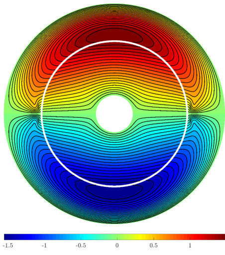
Figure 8. The solution in the interior domains $\Omega_{1}$ and $\Omega_{2}$ for the electric machine of the example in Section 5.2. The equipotential lines are the magnetic field lines.

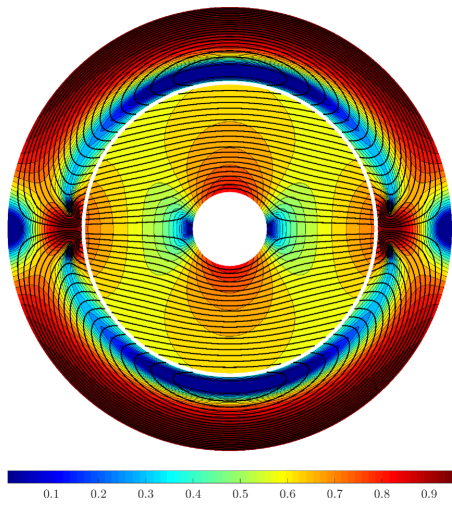
Figure 9. Saturation effects caused by the non-linear material tensors. The color-bar and the thin lines represent the levels of the magnetic reluctivity, which is given by $g(\nabla u_{i}),$ for $i=1,2$, and evaluated using the derivatives of the solutions $u_{1}$ and $u_{2}$. The thick equipotential lines show the flow direction of the magnetic field.

To verify Remark 4.8 numerically, we evaluate the solution in the BEM domain $\Omega_{\mathrm{b}}$ on the evaluation path given as the parametrized circle $\partial B((0,0);0.395)$. Note that in this example, the BEM is applied in an interior domain $\Omega_{\mathrm{b}}$. Hence, we use for the evaluation the representation formula (2) with $\kappa=0$ and the complete Cauchy data on $\Gamma_{1}$ and $\Gamma_{2}$, which are available after solving Problem 4.4 with the jump condition (16c). An analytical solution for our model problem is not known. Hence, to verify the convergence order, we follow a standard procedure: The mesh of the current solution is successively refined three times and we calculate the corresponding discrete solutions. We apply the Aitkin’s $\Delta^{2}$-extrapolation to this sequence of discrete solutions and this extrapolated value is the reference solution $u^{\mathrm{e}}(x_{i})$ for the $\text{error}=\max_{i=1,\ldots,N}|u^{\mathrm{e}}(x_{i})-u^{\mathrm{e}}_{\ell}(x_{i})|$ calculated from $N=20$ evaluations points. This error is visualized in Figure 10 for ansatz spaces of degree $p=2$ and $p=3$, where we observe an amelioration of the convergence rates. Note that this amelioration depends on the quality of the numerical integration, as shown in Figure 6 for the example of Section 5.1. For this example, noticeable amelioration of the convergence rates were only observable for a high number of Gaussian quadrature points. In this case, $N_{\mathrm{Gauss}}=400$ points were considered for the assembling of the BEM matrices, which is very time consuming. The dominance of the quadrature error for this type of evaluations can however be tackled, as mentioned in the previous section, by using special extraction techniques. Moreover, efficient assembly of the BEM matrices based on B-spline tailored quadrature rules, as given in [ACD⁺18], together with suitable compression methods, see e.g., [DKSW19], would accelerate the computation considerably. However, this investigation is beyond the scope of this work.

Figure 10. Convergence of the solution on the evaluation path $\Gamma_{\mathrm{e}}=\partial B((0,0);0.395)$ (circle) in the air gap $\Omega_{\mathrm{b}}$ for the example in Section 5.2. The $\text{error}=\max_{i=1,\ldots,N}|u^{\mathrm{e}}(x_{i})-u^{\mathrm{e}}_{\ell}(x_{i})|$ is calculated with $N=20$ evaluations points on $\Gamma_{\mathrm{e}}$. As a replacement for the unknown analytical solution we use an Aitken $\Delta^{2}$ extrapolation of a sequence of successively refined discrete solutions.

6. Conclusions

The non-symmetric FEM-BEM coupling in the isogeometric context for simulating practical problems with complex geometries turns out to be a promising alternative to classical approaches. A transformation to an integral formulation allows a problem in a domain to be reduced to its boundary, where the BEM can be applied. For exterior problems there is no need to truncate the unbounded domain, and for simulating thin gaps there is no need for a complicated remeshing. In both cases numerical errors can be avoided. Thanks to the definition of B-Splines, $h$- and $p$-refinements are applied in a straightforward manner. Furthermore, multiple domain modeling can be done independently. This is particularly advantageous if we consider moving or deforming geometries. A classical transmission and a multiple domain problem with parts of non-linear material are considered. Obviously, FEM is applied to the non-linear areas, whereas BEM is exclusively used for the linear problem. For both model problems, well-posedness for the continuous and discrete problem, and quasi-optimality and convergence rates for the numerical approximation are mathematically analyzed in the isogeometric framework. Furthermore, we show an improvement of the convergence behavior, if we consider the error in functionals of the solution. This is motivated by a practice-oriented application such as electric machines. Here the computation of torques are a central task and involve the evaluation of some derivatives of the solution in the BEM domain. We observe for both model applications this super-convergence, which confirms the theory. Future extensions of the method may include the consideration of parabolic-elliptic problems and a rigorous analysis of the coupling for $\operatorname{curl}\operatorname{curl}$-type equations in $3$D.

References

• [ACD+18] A. Aimi, F. Calabro, M. Diligenti, M. L. Sampoli, G. Sangalli, and A. Sestini. Efficient assembly based on B-spline tailored quadrature rules for the IgA-SGBEM. Computer Methods in Applied Mechanics and Engineering, 331:327–342, 2018.
• [AFF+13] M. Aurada, M. Feischl, T. Führer, M. Karkulik, J. M. Melenk, and D. Praetorius. Classical FEM-BEM coupling methods: nonlinearities, well-posedness, and adaptivity. Computational Mechanics, 51(4):399–419, 2013.
• [BadVBSV14] L. Beirão da Veiga, A. Buffa, G. Sangalli, and R. Vázquez. Mathematical analysis of variational isogeometric methods. Acta Numerica, 23:157–287, 2014.
• [Ban15] A. Bantle. On high-order NURBS-based boundary element methods in two dimensions-numerical integration and implementation. PhD thesis, Fakultät für Mathematik und Wirtschaftswissenschaften, Universität Ulm, 2015.
• [BBadVC+06] Y. Bazilevs, L. Beirão da Veiga, J. A. Cottrell, T. J. R. Hughes, and G. Sangalli. Isogeometric analysis: approximation, stability and error estimates for h-refined meshes. Mathematical Models and Methods in Applied Sciences, 16(07):1031–1090, 2006.
• [BCSDG17] Z. Bontinck, J. Corno, S. Schöps, and H. De Gersem. Isogeometric Analysis and Harmonic Stator-Rotor Coupling for Simulating Electric Machines. Computer Methods in Applied Mechanics and Engineering, 334, 09 2017.
• [BDK+20] A. Buffa, J. Dölz, S. Kurz, S. Schöps, R. Vázquez, and F. Wolf. Multipatch approximation of the de Rham sequence and its traces in isogeometric analysis. Numerische Mathematik, 144(1):201–236, 2020.
• [BM83] J. Bielak and R. C. MacCamy. An exterior interface problem in two-dimensional elastodynamics. Quarterly of Applied Mathematics, 41(1):143–159, 1983.
• [CdFDGS16] J. Corno, C. de Falco, H. De Gersem, and S. Schöps. Isogeometric simulation of Lorentz detuning in superconducting accelerator cavities. Computer Physics Communications, 201:1–7, 2016.
• [CHB09] J. A. Cottrell, T. JR Hughes, and Y. Bazilevs. Isogeometric analysis: toward integration of CAD and FEA. John Wiley & Sons, 2009.
• [Cos88a] M. Costabel. Boundary integral operators on Lipschitz domains: elementary results. SIAM Journal on Mathematical Analysis, 19(3):613–626, 1988.
• [Cos88b] M. Costabel. A symmetric method for the coupling of finite elements and boundary elements. The Mathematics of Finite Elements and Applications, VI (Uxbridge, 1987), pages 281–288, 1988.
• [dFRV11] C. de Falco, A. Reali, and R. Vázquez. GeoPDEs: a research tool for isogeometric analysis of PDEs. Advances in Engineering Software, 42(12):1020–1034, 2011.
• [DKSW19] J. Dölz, S. Kurz, S. Schöps, and F. Wolf. Isogeometric boundary elements in electromagnetism: Rigorous analysis, fast methods, and examples. SIAM Journal on Scientific Computing, 41(5):B983–B1010, 2019.
• [EES18] H. Egger, C. Erath, and R. Schorr. On the nonsymmetric coupling method for parabolic-elliptic interface problems. SIAM J. Numer. Anal., 56(6):3510–3533, 2018.
• [EOS17] C. Erath, G. Of, and F. Sayas. A non-symmetric coupling of the finite volume method and the boundary element method. Numerische Mathematik, 135(3):895–922, 2017.
• [Era12] C. Erath. Coupling of the finite volume element method and the boundary element method: an a priori convergence result. SIAM J. Numer. Anal., 50(2):574–594, 2012.
• [FGHP16] M. Feischl, G. Gantner, A. Haberl, and D. Praetorius. Adaptive 2D IGA boundary element methods. Engineering Analysis with Boundary Elements, 62:141 – 153, 2016.
• [FGP15] M. Feischl, G. Gantner, and D. Praetorius. Reliable and efficient a posteriori error estimation for adaptive IGA boundary element methods for weakly-singular integral equations. Computer Methods in Applied Mechanics and Engineering, 290:362 – 386, 2015.
• [FGPS19] T. Führer, G. Gantner, D. Praetorius, and S. Schimanko. Optimal additive schwarz preconditioning for adaptive 2D IGA boundary element methods. Computer Methods in Applied Mechanics and Engineering, 351:571 – 598, 2019.
• [Gan14] G. Gantner. Adaptive isogeometrische BEM. Master’s thesis, Vienna University of Technology, 2014.
• [Gan17] G. Gantner. Optimal adaptivity for splines in finite and boundary element methods. PhD thesis, Vienna University of Technology, 2017.
• [HCB05] T.J.R. Hughes, J.A. Cottrell, and Y. Bazilevs. Isogeometric analysis: CAD, finite elements, NURBS, exact geometry and mesh refinement. Computer Methods in Applied Mechanics and Engineering, 194(39):4135 – 4195, 2005.
• [HR09] H. Harbrecht and M. Randrianarivony. From computer aided design to wavelet BEM. Computer Methods in Applied Mechanics and Engineering, 13(2):69 – 82, 2009.
• [JN80] C. Johnson and J. C. Nédélec. On the coupling of boundary integral and finite element methods. Mathematics of computation, 35:1063–1079, 1980.
• [KFK+97] S. Kurz, J. Fetzer, T. Kube, G. Lehner, and W. M. Rucker. BEM-FEM coupling in electromechanics: A 2-D watch stepping motor driven by a thin wire coil. Applied Computational Electromagnetics Society Journal, 12:135–139, 1997.
• [Kur98] S. Kurz. Die numerische Behandlung elektromechanischer Systeme mit Hilfe der Kopplung der Methode der finiten Elemente und der Randelementmethode. VDI-Verlag, 1998.
• [McL00] W. McLean. Strongly elliptic systems and boundary integral equations. Cambridge university press, 2000.
• [MS87] R. C. MacCamy and M. Suri. A time-dependent interface problem for two-dimensional eddy currents. Quart. Appl. Math., 44:675–690, 1987.
• [MZBF15] B. Marussig, J. Zechner, G. Beer, and T.-P. Fries. Fast isogeometric boundary element method based on independent field approximation. Computer Methods in Applied Mechanics and Engineering, 284:458 – 488, 2015. Isogeometric Analysis Special Issue.
• [OS13] G. Of and O. Steinbach. Is the one-equation coupling of finite and boundary element methods always stable? ZAMM-Journal of Applied Mathematics and Mechanics/Zeitschrift für Angewandte Mathematik und Mechanik, 93(6-7):476–484, 2013.
• [OS14] G. Of and O. Steinbach. On the ellipticity of coupled finite element and one-equation boundary element methods for boundary value problems. Numerische Mathematik, 127(3):567–593, 2014.
• [Pec04] C. Pechstein. Multigrid-Newton-methods for nonlinear magnetostatic problems. Master’s thesis, Johannes Kepler University of Linz, Institute of Computational Mathematics, Linz, 2004.
• [PGK+09] C. Politis, A. I. Ginnis, P. D. Kaklis, K. Belibassakis, and C. Feurer. An isogeometric BEM for exterior potential-flow problems in the plane. In 2009 SIAM/ACM Joint Conference on Geometric and Physical Modeling, SPM ’09, page 349–354, New York, NY, USA, 2009. Association for Computing Machinery.
• [PT12] L. Piegl and W. Tiller. The NURBS book. Springer Science & Business Media, 2012.
• [Röm15] U. Römer. Numerical approximation of the magnetoquasistatic model with uncertainties and its application to magnet design. PhD thesis, Institut für Theorie Elektromagnetischer Felder, Technische Universität Darmstadt, 2015.
• [Say09] F. Sayas. The validity of Johnson–Nédélec’s BEM–FEM coupling on polygonal interfaces. SIAM Journal on Numerical Analysis, 47(5):3451–3463, 2009.
• [SS10] S. A. Sauter and C. Schwab. Boundary Element Methods. In Boundary Element Methods, pages 183–287. Springer, 2010.
• [SSE+13] M.A. Scott, R.N. Simpson, J.A. Evans, S. Lipton, S.P.A. Bordas, T.J.R. Hughes, and T.W. Sederberg. Isogeometric boundary element analysis using unstructured T-splines. Computer Methods in Applied Mechanics and Engineering, 254:197 – 221, 2013.
• [Ste07] O. Steinbach. Numerical approximation methods for elliptic boundary value problems: finite and boundary elements. Springer Science & Business Media, 2007.
• [Ste11] O. Steinbach. A note on the stable one-equation coupling of finite and boundary elements. SIAM journal on numerical analysis, 49(4):1521–1531, 2011.
• [SW99] C. Schwab and W. Wendland. On the extraction technique in boundary integral equations. Mathematics of computation, 68(225):91–122, 1999.
• [Zei86] E. Zeidler. Nonlinear Functional Analysis and its Applications II/B: Nonlinear Monotone Operators. Springer, 1986.