Partial local entropy and anisotropy in deep weight spaces

Abstract

We refine a recently-proposed class of local entropic loss functions by restricting the smoothening regularization to only a subset of weights. The new loss functions are referred to as partial local entropies. They can adapt to the weight-space anisotropy, thus outperforming their isotropic counterparts. We support the theoretical analysis with experiments on image classification tasks performed with multi-layer, fully-connected and convolutional neural networks. The present study suggests how to better exploit the anisotropic nature of deep landscapes and provides direct probes of the shape of the minima encountered by stochastic gradient descent algorithms. As a by-product, we observe an asymptotic dynamical regime at late training times where the temperature of all the layers obeys a common cooling behavior.

Departamento de Física de Partículas,
Universidade de Santiago de Compostela (USC)
Instituto Galego de Física de Altas Enerxías (IGFAE)
E-15782 Santiago de Compostela, Spain
and
Inovalabs Digital S.L. (TECHEYE),
E-36202 Vigo, Spain and
Centro de Supercomputación de Galicia (CESGA),
s/n, Avenida de Vigo, 15705 , Santiago de Compostela, Spain

1 Introduction

Recent studies on the weight space of deep neural networks [2, 8] have highlighted the existence of rare subdominant clusters of configurations which yield a high test accuracy. Although these clusters constitute a deviation from typicality, they are efficiently encountered by stochastic gradient descent (SGD) algorithms and correspond to wide valleys of suitable loss functions, such as cross entropy [4].

An analogous circumstance occurs in the context of constraint satisfaction problems, where the chase after clusters of solutions is improved when the loss function gets supplemented by a term that encourages a local high density of solutions [3]. In order to find the number of solutions contained in a vicinity of a specific weight configuration, one can define a local solution-counting functional, namely, a local entropy.

Classification tasks performed by means of quantized neural networks (where the weights are discrete) can be interpreted as constraint satisfaction problems. There are however two reasons to generalize the concept of local entropy: First, classification problems are typically required to reach a high but not necessarily perfect accuracy; second, they are often approached with machines that have continuous weights. The strict counting of solutions employed for constraint satisfaction problems can therefore be relaxed to just an incentive which encourages a high local density of high-accuracy configurations. A local averaging of the loss, for instance, is expected to have such an effect, but other deformations of the loss yielding a local smoothening can be valid choices too.

A specific smoothening procedure of the loss function can be enforced by means of a spatial convolution with an Euclidean heat kernel, whose spread is controlled by a parameter $\gamma$,

$${\cal F}(\beta,\gamma;\bm{W})=-\log\int d^{N}W^{\prime}\ \exp\left(-\beta{\cal L}(\bm{W}^{\prime})-\frac{\gamma}{2}||\bm{W}-\bm{W}^{\prime}||^{2}_{2}\right)\ ,$$ (1)

where both $\bm{W}$ and $\bm{W}^{\prime}$ parametrize the $N$-dimensional weight space, $||.||_{2}$ represents the Euclidean norm and ${\cal L}$ is a generic loss function; adopting an energetic interpretation of the loss, the parameter $\beta$ corresponds to an inverse temperature. In the limit $\beta\rightarrow 0$, the integral in (1) can be interpreted as (the continuum version of) a weighted counting of the configurations $\bm{W}^{\prime}$ where the weighting decreases exponentially with their distance from $\bm{W}$ [1].

The smoothening introduced by (1) is isotropic in weight space. However, when optimizing with SGD, the gradient noise depends in general on both the position and the direction, this being actually a key factor for the success of SGD algorithms [37]. Therefore, it is natural to expect that a refinement of the smoothening functional able to suitably exploit the anisotropy of gradient noise can significantly improve its regularizing effects. Besides, such refinement can furnish an interesting new probe of the weight space.

The present paper focuses on partial, entropic and local smoothening, namely a smoothening analogous to (1) applied to just a subsets of weights. This allows one to address weight-space anisotropy in a direct and active way. We will loosely adopt the term partial local entropy to convey this idea irrespective of the details of the particular smoothening technique, as long as it corresponds to an incentive to local high density of high-accuracy configurations restricted to a subset of weights.

2 Anisotropy in weight space

By definition the neurons of a deep network are arranged on different layers and such architecture imposes a natural hierarchy among them, according to their depth within the network. In a fully-connected setting, the receptive field of each neuron coincides with the whole input, however deeper neurons are fed with signals that have been pre-processed by lower-lying neurons. Roughly, while the neurons in the first layer compute a weighted sum of the network inputs, the neurons in the second layer compute a weighted sum of the outputs of the first layer, that is, a weighted sum of a weighted sum of the network inputs. Such compositional nature of the operation performed by each subsequent layer suggests that the depth of the network corresponds to a hierarchy in combinatorial complexity [14]. Any isotropic assumption about the weight space neglects this structural hierarchy, thereby it should be regarded with caution if not even suspicion.

Careful consideration of the hierarchical anisotropy of the weight space has led to important insight about the inner workings of neural networks (also in the biological domain [30]) as well as improvements in the optimization of artificial neural networks. Gradient noise depends on both position and direction and its covariance matrix is correlated to the Hessian matrix of the loss function, which makes SGD escape exponentially fast from sharp minima [37]. Thus, it is fair to consider weight-space anisotropy as one of the main features at the root of the effectiveness of SGD algorithms in reaching high test accuracy and generalization.

2.1 Layer temperature and asymptotic cooling

The learning dynamics of a deep neural network trained with SGD is in general a complex process. The system is out of equilibrium and, given the dependence of the gradient noise on the position in weight space, one cannot schematize the training as the evolution of a system in contact with an equilibrium thermal reservoir. Nonetheless, it is still possible to define a temperature as the variance of the gradient noise when schematizing the training evolution in terms of a Brownian motion [14, 10, 26]. More precisely, one has to focus on the covariance matrix $D(\bm{W})$ characterizing the stochastic Wiener process.

Let us focus for a moment on a specific point $\bm{W}^{*}$ in weight space. Given the anisotropy of $D(\bm{W}^{*})$, it is impossible to define a unique temperature characterizing all directions, but one can in principle still define a temperature for each direction. Since we are working in a space with very high dimensionality, this is hardly of any help. However, we should recall that there is a natural grouping of the directions in weight space provided by the layered structure of the network. Furthermore, it is possible to define layer variables which average over the weights belonging to the same layer. One can consider fluctuations of such layer variables that, due to the averaging over a layer, are expected to be stabler and reflect the hierarchy of the architecture. Accordingly, one can define a layer temperature corresponding to the variance of such layer averaging of gradients. This corresponds to regarding the layers as if they were the individual units of a neural network; despite being a crude approximation, this could help gaining useful insight about the training dynamics [33].

The layer temperature is a characterization of the noise of the training signal $s_{I}$ through layer $I$, defined as

$$s_{I}=\frac{1}{N_{I}}\sum_{\omega\in\Omega_{I}}||\nabla_{\omega}{\cal L}(\bm{W})||_{2}\ ,$$ (2)

where $\Omega_{I}$ denotes the set of the $N_{I}$ weights connecting the $I$-th layer with its inputs, $||.||_{2}$ represents the Euclidean norm and ${\cal L}(\bm{W})$ is the loss evaluated at the weight configuration $\bm{W}$. The training signals $s_{I}$ and their noise evolve during optimization and it is possible to isolate different regimes in the training dynamics. In [33] the authors observed that a possibly generic dynamic transition occurs when the signal$/$noise ratio switches from being initially dominated by the signal to being later dominated by noise. This occurs quite abruptly (in terms of optimization time) and approximately at the moment when the training signal attains its maximum value, see Figure 1.

The numerical studies that we performed suggest the generic presence of a further dynamic transition, occurring at later stages of the training. This eventual regime is characterized by a sub-exponential decay of both signal and noise for all layers. Interestingly, the sub-exponential contraction of the signal and the noise for all the layers is characterized by a common decaying behavior. At late times, the hierarchy between layers is therefore preserved and gets frozen: the dynamics of all the layers can in fact be described factorizing the common sub-exponential decay.

Interpreting the noise as a temperature and adopting a renormalization group language, the eventual sub-exponential cooling (possibly turning exponential at asymptotically late times) is suggestive of an infrared fix point, where quantities evolve by a common rescaling without distortion at asymptotic low energies. It is relevant to stress that Figure 1 has been obtained without adopting weight-decay regularization. Moreover, we have obtained qualitatively similar results both with ReLU and TanH activation functions; while the former is scale covariant, the latter is not.

As already stressed, even if the layer-wise account gives a very coarse-grained picture of the actual training dynamics, still it confirms the importance of anisotropy throughout the whole training process, including at asymptotic late times where the in-sample loss and the test error have long stabilized.

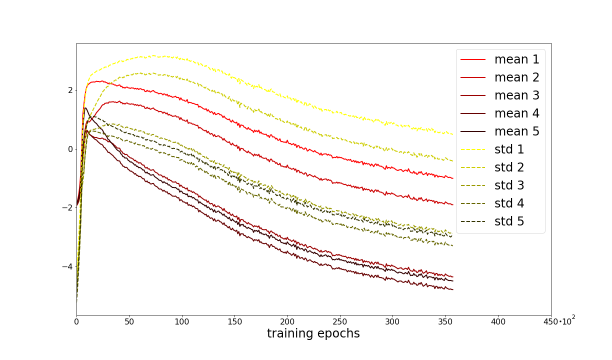
Figure 1: The training signal $s_{I}$ defined in (2) –where $I\in\{1,2,3,4\}$ labels the layers of the network– is represented with solid lines; the dashed lines represent the associated standard deviations. The plots depict a long training of two 4-layer fully-connected neural networks on MNIST with either ReLU (top plot) or TanH (bottom plot) activation functions. Three distinct dynamical regimes emerge in both plots: 1) an early signal-dominated regime; 2) a short, intermediate and noise-dominated regime; 3) an eventual, long and noise-dominated regime where all quantities decay sub-exponentially with a common behavior (the vertical axes are natural logarithms).

3 Partial local free entropy

For the sake of generality, the present section is rather technical. The reader who is just interested in the specific losses used in the experiments can jump to Section 4 and focus on the loss functions (22) and (23) without missing the core ideas.

We consider the cross-entropy loss ${\cal L}_{\text{c.e.}}(\bm{W})$ as the baseline function to be smoothened; $\bm{W}$ is a vector indicating a configuration in weight space. We consider $y$ additional configurations $\bm{W}+\Delta\bm{W}^{a}$ with $a=1,...,y$, shifted by a uniformly distributed random vector $\Delta\bm{W}^{a}$. The loss corresponding to each configuration is supplemented by an additional term measuring its distance from the unperturbed point $\bm{W}$. For the moment we let the distance function $d_{R,k}(\Delta\bm{W}^{a})$ be arbitrary but we assume it depends on two parameters, to be specified later.We consider the new loss

$${\cal M}(R,k,y;\bm{W})\equiv-\log\left\{\frac{1}{y+1}\left[e^{-{\cal L}_{\text{c.e.}}(\bm{W})}+\sum_{a=1}^{y}e^{-{\cal L}_{\text{c.e.}}(\bm{W}+\Delta\bm{W}^{a})-d_{R,k}(\Delta\bm{W}^{a})}\right]\right\}\ ,$$ (3)

normalized with respect to the number of sampling points $y+1$. Roughly, the loss ${\cal M}$ amounts to the logarithm of an average of exponentials. In the case of just one sampling point, $y=0$, ${\cal M}$ coincides with the baseline loss,

$${\cal M}(R,k,y=0;\bm{W})={\cal L}_{\text{c.e.}}(\bm{W})\ .$$ (4)

We choose the following distance function

$$d_{R,k}(\Delta\bm{W})\equiv-\log\prod_{i=1}^{N}\left[\left(1-\frac{1}{1+e^{-2k(\Delta W_{i}-R)}}\right)\frac{1}{1+e^{-2k(\Delta W_{i}+R)}}\right]\ ,$$ (5)

which depends on two real parameters, $R$ and $k$. In the $k\rightarrow\infty$ limit, the kernel

$$K_{R,k}(\Delta\bm{W})\equiv e^{-d_{R,k}(\Delta\bm{W})}\ ,$$ (6)

reduces to the characteristic function of the $N$-dimensional hyper-cube $H_{\bm{W},R}$ centered in $\bm{W}$ with edges $2R$ long,

$$\lim_{k\rightarrow+\infty}K_{R,k}(\Delta\bm{W})=\prod_{i=1}^{N}\left[1-\Theta(\Delta W_{i}-R)\right]\Theta(\Delta W_{i}+R)\ .$$ (8)

Thus, the parameter $R$ represents the effective linear size of the support of the kernel (6), while $k$ controls its sharpness, see Figure 2. In the infinite sharpness limit, $k\rightarrow\infty$, the random displacement vectors $\Delta\bm{W}^{a}$ in (3) are sampling the hyper-cube $H_{\bm{W},R}$ uniformly.

Taking an infinite number of sampling points,

$${\cal M}(R,k,y;\bm{W})\xrightarrow[y\rightarrow+\infty]{}\ {\cal F}(R,k;\bm{W})\ ,$$ (9)

where

$${\cal F}(R,k;\bm{W})\equiv-\log\int d^{N}W^{\prime}\ e^{-{\cal L}_{\text{c.e.}}(\bm{W}^{\prime})}\ K_{R,k}(\bm{W}^{\prime}-\bm{W})\ ,$$ (10)

defines a parametric family ${\cal F}(R,k;\bm{W})$ of local free entropies, in analogy with (1). Taking the $k\rightarrow\infty$ limit of (10), one obtains

$$\lim_{k\rightarrow+\infty}{\cal F}(R,k;\bm{W})=-\log\int_{H_{\bm{W},R}}d^{N}W^{\prime}\ e^{-{\cal L}_{\text{c.e.}}(\bm{W}^{\prime})}\ .$$ (12)

To recapitulate, in the limit of large number of sampling points, $y\rightarrow\infty$, the loss function ${\cal M}(R,k,y;\bm{W})$ approximates a parametric family of free local entropy functions (10) parametrized by the effective linear size $R$ of the smoothening region (in weight-space) and the sharpness $k$ of the associated kernel (6).

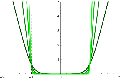
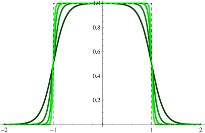
Figure 2: 1-dimensional section of the distance function $d_{R,k}$ defined in (5) (left plot) and of the kernel $K_{R,k}$ defined in (6) (right plot); in the plots $R=1$ and $k=2^{2},2^{3},2^{4},2^{5}$ from darker to lighter.

In order to define partial local free entropies we have just to generalize the passages above to the case where only a subset of weights is smoothened over. We can define a discrete indicator function $\bm{U}$ taking values in $\{0,1\}^{N}$ and defined on the $N$ dimensions of weight space: it takes value $1$ on the directions along which we smoothen the loss, and $0$ on the remaining directions in weight space. Thinking to $\bm{U}$ as an $N$-dimensional vector, it provides an un-normalized projector onto the subset of weights considered for smoothening. We can thus define a restricted version of the distance function $d_{R,k}(\Delta\bm{W})$,

$$d_{R,k}^{[\bm{U}]}(\Delta\bm{W})\equiv d_{R,k}\Big{(}(\Delta\bm{W}\cdot\bm{U})\,\bm{U}\Big{)}\ ,$$ (13)

where $\cdot$ indicates the scalar product of $\mathbb{R}^{N}$ in the $N$-dimensional weight space.

Adopting the restricted distance (13), we can repeat the same steps as above: first consider

$${\cal M}^{[\bm{U}]}(R,k,y;\bm{W})\equiv-\log\left\{\frac{1}{y+1}\left[e^{-{\cal L}_{\text{c.e.}}(\bm{W})}+\sum_{a=1}^{y}e^{-{\cal L}_{\text{c.e.}}(\bm{W}+\Delta\bm{W}^{a})-d_{R,k}^{[\bm{U}]}(\Delta\bm{W}^{a})}\right]\right\}\ ,$$ (14)

then take the $y\rightarrow\infty$ limit

$${\cal M}^{[\bm{U}]}(R,k,y;\bm{W})\xrightarrow[y\rightarrow+\infty]{}\ {\cal F}^{[\bm{U}]}(R,k;\bm{W})\ ,$$ (15)

where

$${\cal F}^{[\bm{U}]}(R,k;\bm{W})\equiv-\log\int d^{N}W^{\prime}\ e^{-{\cal L}_{\text{c.e.}}(\bm{W}^{\prime})}\ K_{R,k}^{[\bm{U}]}(\bm{W}^{\prime}-\bm{W})\ ,$$ (16)

represents a parametric family of partial local free entropies. Eventually, take the $k\rightarrow\infty$ limit,

$${\cal F}^{[\bm{U}]}(R;\bm{W})\equiv\lim_{k\rightarrow+\infty}{\cal F}^{[\bm{U}]}(R,k;\bm{W})\ ,$$ (17)

where

$${\cal F}^{[\bm{U}]}(R;\bm{W})\equiv-\log\int_{H_{\bm{W},R}^{[\bm{U}]}}d^{N}W^{\prime}\ e^{-{\cal L}_{\text{c.e.}}(\bm{W}^{\prime})}\ ;$$ (18)

the integration region $H_{\bm{W},R}^{[\bm{U}]}$ is a hyper-cube extended only in the directions along which $\bm{U}$ is non-null.

3.1 A simpler entropic loss

It is interesting to seek for a simpler loss which could somehow preserve the smoothening effect of partial local free entropy. To this purpose, one can define an averaged loss over an $N$-dimensional vicinity in weight space –this imitating the effects of local entropy– or to a lower-dimensional vicinity – this instead imitating partial local entropy. We focus on the latter case and define

$$\bar{\cal L}^{[\bm{U}]}(R,k,y;\bm{W})\equiv\frac{1}{y+1}\left[{\cal L}_{\text{c.e.}}(\bm{W})+\sum_{a=1}^{y}{\cal L}_{\text{c.e.}}(\bm{W}+\Delta\bm{W}^{a})K_{R,k}^{[\bm{U}]}(\Delta\bm{W}^{a})\right]\ .$$ (19)

Considering the $k\rightarrow\infty$ limit one obtains

$$\bar{\cal L}^{[\bm{U}]}(R,y;\bm{W})\equiv\frac{1}{y+1}\left[{\cal L}_{\text{c.e.}}(\bm{W})+\sum_{a=1}^{y}{\cal L}_{\text{c.e.}}(\bm{W}+\Delta^{[\bm{U}]}\bm{W}^{a})\right]\ ,$$ (20)

where $\Delta^{[\bm{U}]}$ means simply that the random vectors are sampled uniformly within the hyper-cube $H_{\bm{W},R}^{[\bm{U}]}$ centered in $\bm{W}$ and extending along the direction indicated by the vector $\bm{U}$, its edges being $2R$ long. In the limit of infinite samples, we have

$$\bar{\cal L}^{[\bm{U}]}(R;\bm{W})\xrightarrow[y\rightarrow+\infty]{}\ \int_{H_{\bm{W},R}^{[\bm{U}]}}d^{N}W^{\prime}\ {\cal L}_{\text{c.e.}}(\bm{W}^{\prime})\ ,$$ (21)

and the loss reduces to a simple local average along a subset of directions in weight space.

4 Experiments with fully-connected networks

The focus of the first group of experiments is on layer-wise partial entropy regularizations for multi-layer, fully-connected neural networks trained on image classification tasks. Namely, we considered partial local entropies where the subset of weights chosen for smoothening coincides with whole layers. We consider the $10$-class classification tasks associated with MNIST [21] and Fashion-MNIST [36] datasets, whose input images are $28$ pixels wide and $28$ pixels height. We consider both 2-layer and 3-layer fully-connected neural networks with continuous weights having a further $10$-neuron output layer. All layers except the last have $784=28^{2}$ neurons and are structurally identical, apart from their different depth within the network. The following hyper-parameters have been kept fixed for all the experiments: learning rate $\eta=0.0001$, momentum $\mu=0.9$, mini-batch size $256$ and trained for $120$ epochs.

We considered two loss functions, a partial local exponential average loss (PLEA)

$${\cal L}_{\text{PLEA}}(\bm{W})=-\log\left\{\frac{1}{1+y}\left[e^{-{\cal L}_{\text{c.e.}}(\bm{W})}+\sum_{a=1}^{y}e^{-{\cal L}_{\text{c.e.}}(\bm{W}+\Delta\bm{W}^{a})}\right]\right\}\ ,$$ (22)

and a partial local average loss (PLA)

$${\cal L}_{\text{PLA}}(\bm{W})=\frac{1}{1+y}\left[{\cal L}_{\text{c.e.}}(\bm{W})+\sum_{a=1}^{y}{\cal L}_{\text{c.e.}}(\bm{W}+\Delta\bm{W}^{a})\right]\ ,$$ (23)

where ${\cal L}_{\text{c.e.}}$ is the cross-entropy loss and $\Delta\bm{W}^{a}$ is a random vector sampled in a vicinity of $\bm{W}$. Such a vicinity is a hyper-cube centered in $\bm{W}$ with edge $2R$ and extending only along a subspace of the $N$-dimensional weight space. Notice that in this way the regularizations of the cross-entropy ${\cal L}_{\text{c.e.}}$ given by (22) and (23) enforce an anisotropic bias.

In the experiments reported below we consider only subspaces associated to one or more layers at a time. Apart from the entropic smoothening, we do not enforce any further regularization, in particular we do not use weight decay.

4.1 Results

The experiments suggest two main conclusions:

• In general, the entropic regularizations (22) and (23) improve test accuracy. The effect increases rapidly with the size $R$ of the smoothening region, up to a maximum size beyond which performance gets degraded.

• When implemented on suitable subsets of weights (e.g. single layers), the entropic regularizations outperform significantly their isotropic counterparts.

The first point means that smoothening improves performance up to a point beyond which its averaging effect distorts the original loss landscape too heavily. The second point means that the strong differences in the role played by the various weights affect the loss landscape and the effectiveness of regularization. This implies that the shape of the wide flat minima encountered by SGD optimization is relevant, not only their extension. Another generic conclusion suggested by the experiments is that the layer-wise entropic regularization is more effective when performed on deeper levels. This harmonizes with the intuitive idea that deeper weights are associated to more complex features, which –in a reliable classification– should be progressively more robust.

An important detail of the experimental setups is that all layers have the same number of neurons, $784$. Thus, when comparing quantities associated to different layers, we are actually probing the mere effect of depth. A direct comparison between structurally different layers would instead be more difficult to interpret.

4.2 2-layer fully-connected neural network on Fashion-MNIST

We considered 2-layer, fully-connected neural networks adopting both PLEA loss function (22) and PLE loss function (23). The results obtained with the two loss functions are qualitatively analogous.

We measured the test accuracy reached by three versions of the same 2-layer network as we moved the regularization radius $R$, the three versions differ simply by the choice of the weight subspace considered for smoothening: either (i) the whole first layer; (ii) the whole second layer; (iii) both layers (isotropic choice). The results are reported in Figure 3 and Figure 4 (left plot). Regularization on the 2nd layer alone proved to be the best strategy for both choices of loss functions and in the entire range of $R$ probed by the experiments. The isotropic regularization can outperform the regularization on the 1st layer alone, but only at very small values for $R$. In fact, the isotropic choice leads soon to degraded results as $R$ increases, while the single-layer regularizations continue to improve the test accuracy, showing a saturating behavior.

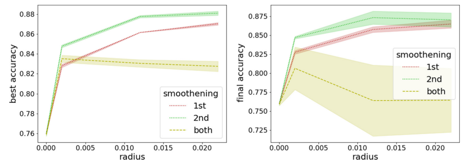
Figure 3: Comparison of the best (left) and final (right) test accuracy reached by a 2-layer fully-connected neural network on Fashion-MNIST. The lines correspond to three different PLA losses (see (23)) obtained by smoothening the cross entropy respectively on the 1st, the 2nd or both layers.

4.3 3-layer fully-connected neural network on MNIST

The experiments on the 3-layer fully-connected neural networks confirm and extend the results obtained for its 2-layer counterpart. They are depicted in 4 (right plot). In particular, the isotropic choice proves to be the worst among all the possible choices of subsets as soon as the smoothening radius $R$ is sufficiently big. Moreover, there is an articulated interplay of regimes as $R$ varies: at the lowest values of $R$ the best choice consists in regularizing with respect to the 1st and 3rd layers jointly; at large values of $R$, regularizing with respect to the 2nd or 3rd layer alone proves to be the best choice. Also the performance hierarchy among the sub-optimal regularization schemes changes as $R$ moves showing a complicated structure.

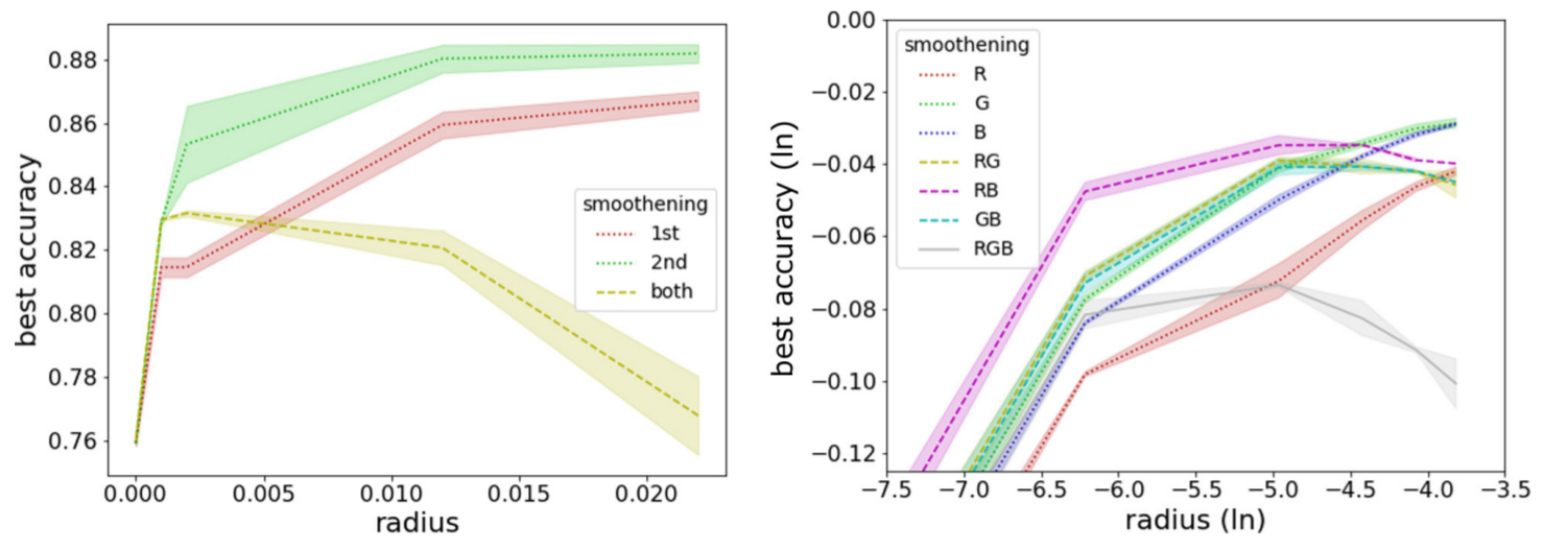
Figure 4: Left plot: best test accuracy reached during training by a 2-layer fully-connected neural network over Fashion-MNIST. The three lines correspond to three different PLEA regularization schemes (see Eq.(3) where smoothening is performed on the 1st layer alone, on the 2nd layer alone or on both layers, respectively. Right plot: best test accuracy reached by a 3-layer fully-connected neural network on MNIST. The lines represents different PLA regularization schemes according to an RGB color nomenclature where Red corresponds to the 1st layer, Green to the 2nd and Blue to the 3rd.

4.4 Finer sampling

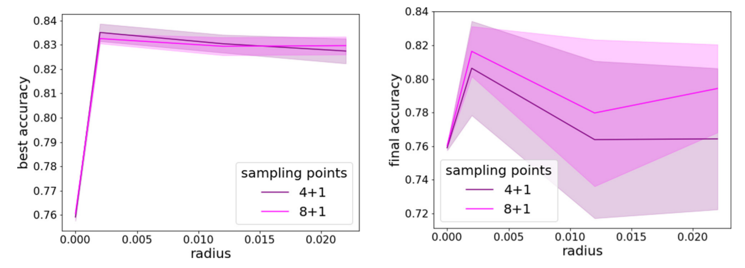
Figure 5: Comparison of the test accuracy performance obtained with a bi-layer fully-connected neural network on Fashion-MNIST and trained with PLA loss (see Eq.(23)). The lighter line refer to finer sampling, $y=8$, while the darker line refers to $y=4$. There is no strong sensitivity to the sample size.

In order to test whether the decrease in accuracy associated to regularizing on multiple layers is due to insufficient sampling (i.e. too small $y$, see (22) and (23)) we repeated the experiments performed with the 2-layer fully-connected neural network on Fashion-MNIST with PLA loss doubling the number of sampling points $y$. The results obtained with $y=8$ are comparable to those obtained with $y=4$, see Figure 5; this hints to the fact that the sampling of the smoothening neighborhood can not explain the poor performance of multi-layer regularization.

5 Experiments with convolutional neural networks

We extend the analysis described in Section 4 in two directions: i) we consider more complicated image classification tasks; ii) we consider deeper networks with convolutional architectures. The convolutional neural networks that we adopt present 5 convolutional layers followed by 3 fully-connected layers, the detail of the architectures are given in (24) and (25). All the convolutional kernels are $3\times 3$.

5.1 Results

The main conclusions which emerged from the study of partial entropic regularizations applied to convolutional neural networks are the following:

1. Partial entropic regularizations involving the convolutional layers lead, in general, to worse classification accuracy with respect to the non-regularized case;

2. When applied to the fully-connected head of convolutional networks, partial entropic regularizations can improve the classification accuracy in a similar way as observed on multi-layered perceptrons, described in Section 4. Especially when adopting an early stopping strategy interrupting training before its full stabilization.

Some further comments are in order. Convolutional layers implement a structured bias encoding some degree of locality and translational invariance. Thus the convolutional structure, if compared to fully-connected layers, is highly specialized. Entropic regularizations can in general be thought of as corresponding to the integration over some injected artificial noise, as such, one expects them to weakens, if not even to spoil, any specific bias previously encoded in the neural architecture. Such comment holds both for the partial entropic regularization studied here, as well as for other forms of noisy regularizations, like Dropout. This latter, too, has been observed to hamper the performance of convolutional networks [13]. Conversely, fully-connected layers have no specific structure and the average over additional noise can lead to better performance in general, also when applied to the fully-connected head in a convolutional network.

In the experiments detailed below, we consider fully-connected heads formed by three layers. The deepest layer outputs 10 channel, as required by the 10-class classification tasks considered and we do not regularize it. The other two fully-connected layers are instead equal in shape among themselves. As already argued in Section 4 for the multi-layer perceptrons, the structural equality allows for a direct comparison between the two layers.

5.2 CIFAR10

For the classification task corresponding to the CIFAR10 dataset we considered the following convolutional architecture:

$$\begin{array}[]{c|c|c}\text{layer}&\text{in channels}&\text{out channels}\\ \hline\cr\text{Conv}&3&64\\ \text{Conv}&64&64\\ \hline\cr\text{MaxPool}&&\\ \hline\cr\text{Conv}&64&128\\ \text{Conv}&128&128\\ \text{Conv}&128&128\\ \hline\cr\text{MaxPool}&&\\ \hline\cr\text{Fully}&128\cdot 4\cdot 4&128\cdot 4\cdot 4\\ \text{Fully}&128\cdot 4\cdot 4&128\cdot 4\cdot 4\\ \text{Fully}&128\cdot 4\cdot 4&10\\ \hline\cr\end{array}$$ (24)

We have trained it for 360 epochs with a constant learning rate $\eta=10^{-4}$, a mini-batch size of 256 images and momentum $\mu=0.9$ without Nesterov acceleration. The training dataset has been augmented/regulated by means of random transformations on the images, specifically we have considered rescaled random crops ranging from $60\%$ to $100\%$ of the image area and with a height/width ratio form $\frac{3}{4}$ to $\frac{4}{3}$. Neither weight decay, nor dropout layers have been used. Actually, the only regularization for the stochastic gradient descent has been provided by the partial local average, encoded in (23), with 4 additional sample points drawn from a uniform distribution in hypercube ball of side equal to $2R$, with $R=0.01$. The initialization followed the so-called Kaiming procedure described in [17].

The results are depicted in Figure 6. We considered three cases: no regularization or PLA regularization applied to either the first or second layer in the fully-connected head (see (24)). The PLA modification of the loss function yields better performance, both in-sample and out-of-sample, especially if combined with an early stopping strategy which interrupts the training before its eventual stabilization. The PLA procedure implies collecting multiple samples of the loss function in the vicinity of the current weight configuration of the network (we took 4 points in a hypercubic vicinity plus the center); the gradient is accumulated but eventually rescaled in such a way that the multiple sampling does not affect the training by means of a simple amplification of the learning rate.

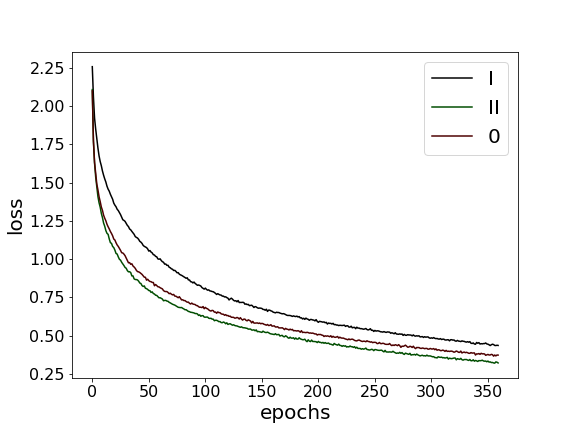
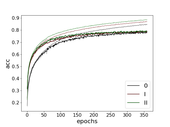
Figure 6: Training loss (left) and test accuracy (right) of the convolutional network (24) trained to solve the CIFAR10 image classification task. The black lines refer to the case where no entropic regularization was considered. The red and green lines refers to PLA (see (23)) loss applied to the first (I) or second (II) fully-connected layer, respectively, as specified in the legend. The paler lines in the right plot depict the in-sample accuracy.

5.2.1 Comparison against standard weight-decay regularization

In order to better assess the effects of partial entropic regularization, we considered comparing them with those produced by a standard regularization method, namely, weight decay [19]. Specifically, we considered three levels of weight decay rate, 0.01, 0.001 and 0.0001. As shown in Figure 7, weight decay regularization proved to be of essentially no utility in the present experiments. On the contrary, partial entropic regularization proved to improve the performance, more significantly in the early phase of the training, only slightly in later stages. These experiments do not pretend to support a generic claim, however they show explicitly that partial entropic regularization can be preferable with respect to weight regularization.

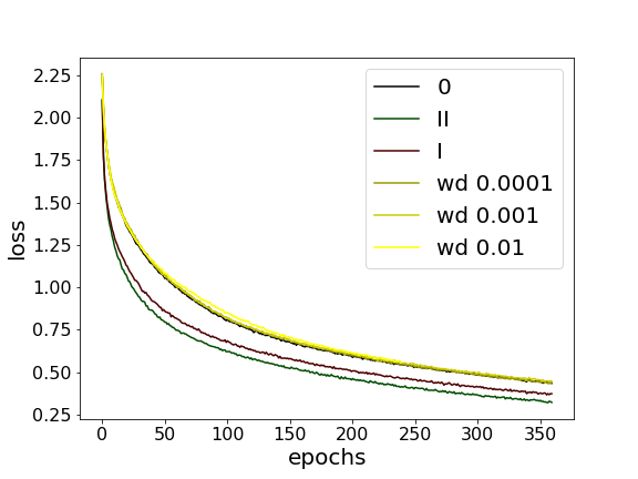
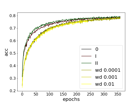
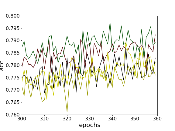
Figure 7: The paler (yellow) lines represent training instances which adopted increasing levels of weight decay regularization, 0.01, 0.001 and 0.0001, respectively from darker to lighter. They all overlap with the unregularized case (label 0), meaning that the effects of weight regularization are irrelevant. The plot on the top left depicts the in-sample loss during training on CIFAR10; the lowest line corresponds to II and the second from below corresponds to I. The plot on the top right shows the out-of-sample accuracy during training on CIFAR10; the uppermost line corresponds to II while the second from top corresponds to I. The bottom plot is a zoom of the top right figure highlighting the late portion of the training.

5.3 STL10

STL10 is a 10-class classification dataset of $96\times 96$ color images acquired from ImageNet. STL10 was designed for partially unsupervised learning [11], in fact it contains only 500 labeled images for supervised training. Although these hardly suffice to train a machine in a fully supervised setup, we use them to simply show the positive effects that partial entropy regularizations induce on the early phase of the training, without requiring an overall satisfactory performance.

We adopt the following convolutional architecture

$$\begin{array}[]{c|c|c}\text{layer}&\text{in channels}&\text{out channels}\\ \hline\cr\text{Conv}&3&8\\ \text{Conv}&8&8\\ \hline\cr\text{MaxPool}&&\\ \hline\cr\text{Conv}&8&16\\ \text{Conv}&16&16\\ \text{Conv}&16&16\\ \hline\cr\text{MaxPool}&&\\ \hline\cr\text{Fully}&16\cdot 20\cdot 20&16\cdot 20\cdot 20\\ \text{Fully}&16\cdot 20\cdot 20&16\cdot 20\cdot 20\\ \text{Fully}&16\cdot 20\cdot 20&10\\ \hline\cr\end{array}$$ (25)

which is analogous to (24), but has lighter layers. We trained it for 960 epochs with a constant learning rate $\eta=10^{-5}$, momentum $\mu=0.9$ without Nesterov acceleration and a mini-batch size of $64$ images. In order to mitigate the issue presented by the smallness of the training set, we have applied heavy augmentation and regularization to the training images. Specifically, we considered random crops whose size ranges from $8\%$ to the full image, and whose aspect ratio ranges from $\frac{3}{4}$ to $\frac{4}{3}$; we considered random horizontal flips, random reduction to gray-scale (with a probability $p=0.1$), color jitter (brightness, contrast, saturation and hue all set to $0.5$) and random rotation whose maximal rotation angle is $\pm\pi$ radiants.

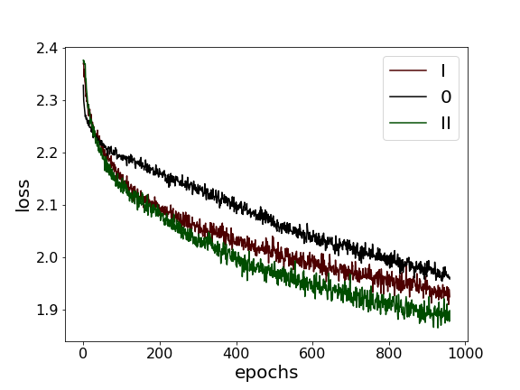
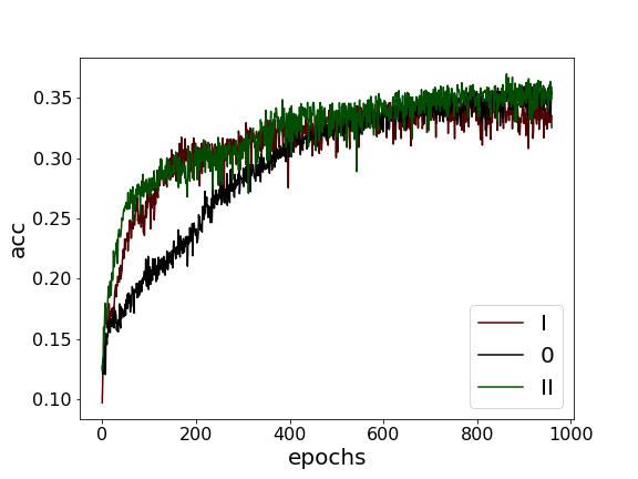
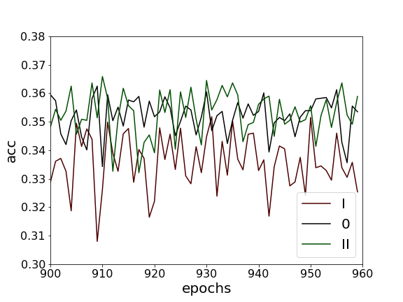
Figure 8: Training loss (left) and test accuracy (right) of a deep convolutional network (25) trained on the STL10 image dataset in a fully supervised scheme for 960 epochs. The black lines correspond to zero entropic regularization, while the lines I and II correspond to partial entropic regularization applied only to the 1st and 2nd fully-connected layers, respectively. The green line (II) correspond to lowest loss and highest accuracy. The bottom plot is a zoom over the last part of the right plot above, depicting the accuracy levels reached at the end of the training.

We monitored the training and report the evolution of the in-sample loss and the test accuracy in Figure 8. The partial entropic regularization, applied to one layer at a time, improves the training and validation performances, but only if accompanied with an early stopping strategy. The experiments of Figure 8 refer to a PLA loss (23) where the side of the sampled hypercube is $2R$ with $R=0.01$. The network was initialized according to the Kaiming method [17], no weight decay was considered.

6 Discussion

A local smoothening of the loss function can improve the chase for wide flat minima [2, 8], which is already a strength of the standard stochastic gradient descent algorithm [37]. We elaborate and refine the smoothening techniques based on local entropy to the purpose of leveraging the anisotropic nature of deep weight spaces. Concretely, we propose to restrict local entropic losses to suitable sub-spaces of weights, thus defining partial local entropies. This allows us to explore, address and exploit the intrinsic anisotropic nature of deep weight spaces. In fact, we show that a partial entropic regularization can implement useful biases on the shape of the minima encountered by SGD optimization.

We have mainly explored the layer-wise implementations of partial local entropies; although there is room for finer analyses resolving smaller sub-spaces, the layer-wise approach is both natural (i.e. well-adapted to the architecture of deep networks) and informative.

In the present paper we have applied partial entropic regularizations to some fully-connected and convolutional neural networks employed for image classification tasks, they can however be employed for the optimization of wider classes of learning machines, e.g. auto-encoders [27]. In particular, the specific layer-wise entropic regularizations proposed in the present study apply in any context involving a layered neural network. The partial entropic regularizations have been proved to be potentially useful in all the considered experiments. However, their positive effects in progressively more demanding tasks seem to be restricted to an early stopping protocol. The adoption of a partial entropic loss led to a more aggressive optimization in all the performed experiments.

6.1 Direct analysis in the language of statistical physics

The study of local entropic regularizations is a very active research front in machine learning, especially in connection to statistical physics [38, 2, 9, 1, 3, 4, 27, 5, 28]. Wide flat minima have been described as a structural characteristic of deep networks and their correlation with good generalization performance has been claimed in [2, 4]. In some simple setups, it is even possible to estimate analytically the hyper-volume of the clusters of configurations giving rise to the relevant minima [6, 4]. The theoretical framework on which the calculations are based has been developed for the study of disordered systems in condensed matter, mainly spin glasses (see [24] and references therein), it is called replica approach. Within this approach, different regimes are described by different ansatzes and can be separated by clustering transitions [7].

A simple version of the replica approach [23] can rely on two (crude) assumptions: (i) averaging over (typically Gaussian) input; (ii) considering tree-like architectures. The former essentially washes out completely the information about the dataset. This is not always undesirable, in fact it allows for the characterization of structural properties of the machines that hold true per se independently of the dataset. It however constitutes a limitation whenever the actual information provided by the input is important. As a future prospect, it would be interesting to study how a direct and explicit account of correlations in the input data could improve the theoretical understanding of the partial entropic regularizations, especially regarding their effects on the inference quality. Considering a tree-like architecture is very helpful to simplify the computations, in fact avoiding loops in the network often opens the possibility of exact computations by, for instance, belief propagation algorithms [23, 4]. Nevertheless, adopting a tree-like network as a proxy for a fully-connected one can be too crude a simplification which is expected to deviate more significantly as the depth of the system is increased.

In order to explain the experiments described in Section 4, it would be desirable to have a direct control on the shape of the relevant clusters of weight configurations reached upon SGD training, or at least an estimation thereof. This could be seen as a refinement of the estimation of the clusters size [6, 4], as such it is likely to be a very demanding endeavor up to the point that it becomes natural to ask whether some simpler –though possibly rougher– approach is viable. To this purpose, it is interesting to investigate mean-field inference methods [15].

7 Acknowledgements

I would like to thank Riccardo Argurio, Diogo Buarque Franzosi, Stefano Goria, Javier Más, Andrea Mezzalira, Giorgio Musso, Alfonso Ramallo, Hernán Serrano and Maurice Weiler for interesting discussions.

References

- [1] Carlo Baldassi, Christian Borgs, Jennifer T. Chayes, Alessandro Ingrosso, Carlo Lucibello, Luca Saglietti, and Riccardo Zecchina. Unreasonable effectiveness of learning neural networks: From accessible states and robust ensembles to basic algorithmic schemes. Proceedings of the National Academy of Sciences, 113(48):E7655–E7662, Nov 2016.
- [2] Carlo Baldassi, Alessandro Ingrosso, Carlo Lucibello, Luca Saglietti, and Riccardo Zecchina. Subdominant dense clusters allow for simple learning and high computational performance in neural networks with discrete synapses. Physical review letters, 115 12:128101, 2015.
- [3] Carlo Baldassi, Alessandro Ingrosso, Carlo Lucibello, Luca Saglietti, and Riccardo Zecchina. Local entropy as a measure for sampling solutions in constraint satisfaction problems. Journal of Statistical Mechanics: Theory and Experiment, 2016:023301, 2016.
- [4] Carlo Baldassi, Enrico M. Malatesta, and Riccardo Zecchina. Properties of the geometry of solutions and capacity of multilayer neural networks with rectified linear unit activations. Physical Review Letters, 123(17), Oct 2019.
- [5] Carlo Baldassi, Riccardo Della Vecchia, Carlo Lucibello, and Riccardo Zecchina. Clustering of solutions in the symmetric binary perceptron, 2019.
- [6] E. Barkai, D. Hansel, and I. Kanter. Statistical mechanics of a multilayered neural network. Phys. Rev. Lett., 65:2312–2315, Oct 1990.
- [7] Tommaso Castellani and Andrea Cavagna. Spin-glass theory for pedestrians. Journal of Statistical Mechanics: Theory and Experiment, 2005(05):P05012, May 2005.
- [8] Pratik Chaudhari, Anna Choromanska, Stefano Soatto, Yann LeCun, Carlo Baldassi, Christian Borgs, Jennifer Chayes, Levent Sagun, and Riccardo Zecchina. Entropy-SGD: Biasing Gradient Descent Into Wide Valleys. arXiv e-prints, page arXiv:1611.01838, November 2016.
- [9] Pratik Chaudhari, Anna Choromanska, Stefano Soatto, Yann LeCun, Carlo Baldassi, Christian Borgs, Jennifer Chayes, Levent Sagun, and Riccardo Zecchina. Entropy-sgd: Biasing gradient descent into wide valleys, 2016.
- [10] Pratik Chaudhari and Stefano Soatto. Stochastic gradient descent performs variational inference, converges to limit cycles for deep networks. CoRR, abs/1710.11029, 2017.
- [11] Adam Coates, Honglak Lee, and Andrew Ng. An analysis of single-layer networks in unsupervised feature learning. pages 1–9, 01 2011.
- [12] P.C. [da Silva], L.R. [da Silva], E.K. Lenzi, R.S. Mendes, and L.C. Malacarne. Anomalous diffusion and anisotropic nonlinear fokker–planck equation. Physica A: Statistical Mechanics and its Applications, 342(1):16 – 21, 2004. Proceedings of the VIII Latin American Workshop on Nonlinear Phenomena.
- [13] Terrance DeVries and Graham W. Taylor. Improved regularization of convolutional neural networks with cutout, 2017.
- [14] Weinan E. A proposal on machine learning via dynamical systems. Communications in Mathematics and Statistics, 5:1–11, 02 2017.
- [15] Marylou Gabrié. Mean-field inference methods for neural networks. Journal of Physics A: Mathematical and Theoretical, 53(22):223002, May 2020.
- [16] Ziv Goldfeld, Ewout van den Berg, Kristjan Greenewald, Igor Melnyk, Nam Nguyen, Brian Kingsbury, and Yury Polyanskiy. Estimating information flow in deep neural networks, 2019.
- [17] Kaiming He, Xiangyu Zhang, Shaoqing Ren, and Jian Sun. Delving deep into rectifiers: Surpassing human-level performance on imagenet classification, 2015.
- [18] Y Kabashima. Inference from correlated patterns: a unified theory for perceptron learning and linear vector channels. Journal of Physics: Conference Series, 95:012001, Jan 2008.
- [19] Anders Krogh and John A. Hertz. A simple weight decay can improve generalization. In Proceedings of the 4th International Conference on Neural Information Processing Systems, NIPS’91, page 950–957, San Francisco, CA, USA, 1991. Morgan Kaufmann Publishers Inc.
- [20] Florent Krzakała, Andrea Montanari, Federico Ricci-Tersenghi, Guilhem Semerjian, and Lenka Zdeborová. Gibbs states and the set of solutions of random constraint satisfaction problems. Proceedings of the National Academy of Sciences, 104(25):10318–10323, 2007.
- [21] Y. Lecun, L. Bottou, Y. Bengio, and P. Haffner. Gradient-based learning applied to document recognition. Proceedings of the IEEE, 86(11):2278–2324, Nov 1998.
- [22] Qianli Liao, Brando Miranda, Lorenzo Rosasco, Andrzej Banburski, Robert Liang, Jack Hidary, and Tomaso Poggio. Generalization puzzles in deep networks, 2020.
- [23] M. Mézard and A. Montanari. Information, Physics, and Computation. Oxford Graduate Texts. OUP Oxford, 2009.
- [24] M. Mezard, G. Parisi, and M.A. Virasoro. Spin Glass Theory And Beyond: An Introduction To The Replica Method And Its Applications. World Scientific Lecture Notes In Physics. World Scientific Publishing Company, 1987.
- [25] M. Mézard, G. Parisi, and R. Zecchina. Analytic and algorithmic solution of random satisfiability problems. Science, 297(5582):812–815, 2002.
- [26] Daniele Musso. Stochastic gradient descent with random learning rate. 3 2020.
- [27] Matteo Negri, Davide Bergamini, Carlo Baldassi, Riccardo Zecchina, and Christoph Feinauer. Natural representation of composite data with replicated autoencoders, 2019.
- [28] Fabrizio Pittorino, Carlo Lucibello, Christoph Feinauer, Enrico M. Malatesta, Gabriele Perugini, Carlo Baldassi, Matteo Negri, Elizaveta Demyanenko, and Riccardo Zecchina. Entropic gradient descent algorithms and wide flat minima, 2020.
- [29] Tomaso Poggio, Andrzej Banburski, and Qianli Liao. Theoretical issues in deep networks. Proceedings of the National Academy of Sciences, 117(48):30039–30045, 2020.
- [30] Maximilian Riesenhuber and Tomaso Poggio. Riesenhuber, m. and poggio, t. hierarchical models of object recognition in cortex. nat. neurosci. 2, 1019-1025. Nature neuroscience, 2:1019–25, 12 1999.
- [31] Andrew Michael Saxe, Yamini Bansal, Joel Dapello, Madhu Advani, Artemy Kolchinsky, Brendan Daniel Tracey, and David Daniel Cox. On the information bottleneck theory of deep learning. In International Conference on Learning Representations, 2018.
- [32] Utkarsh Sharma and Jared Kaplan. A neural scaling law from the dimension of the data manifold, 2020.
- [33] Ravid Shwartz-Ziv and Naftali Tishby. Opening the black box of deep neural networks via information. CoRR, abs/1703.00810, 2017.
- [34] Samuel L. Smith and Quoc V. Le. A Bayesian Perspective on Generalization and Stochastic Gradient Descent. arXiv e-prints, page arXiv:1710.06451, October 2017.
- [35] Maurice Weiler and Gabriele Cesa. General -equivariant steerable cnns, 2019.
- [36] Han Xiao, Kashif Rasul, and Roland Vollgraf. Fashion-mnist: a novel image dataset for benchmarking machine learning algorithms, 2017.
- [37] Zeke Xie, Issei Sato, and Masashi Sugiyama. A diffusion theory for deep learning dynamics: Stochastic gradient descent escapes from sharp minima exponentially fast. ArXiv, abs/2002.03495, 2020.
- [38] Sixin Zhang, Anna Choromanska, and Yann LeCun. Deep learning with elastic averaging sgd, 2014.
- [39] Zhanxing Zhu, Jingfeng Wu, Bing Yu, Lei Wu, and Jinwen Ma. The Anisotropic Noise in Stochastic Gradient Descent: Its Behavior of Escaping from Sharp Minima and Regularization Effects. arXiv e-prints, page arXiv:1803.00195, February 2018.