Impact of LHC vector boson production in heavy ion collisions on strange PDFs

Abstract

The extraction of the strange quark parton distribution function (PDF) poses a long-standing puzzle. Measurements from neutrino-nucleus deep inelastic scattering (DIS) experiments suggest the strange quark is suppressed compared to the light sea quarks, while recent studies of $W^{\pm}\!/Z$ boson production at the LHC imply a larger strange component at small $x$ values. As the parton flavor determination in the proton depends on nuclear corrections, e.g. from heavy-target DIS, LHC heavy ion measurements can provide a distinct perspective to help clarify this situation. In this investigation we extend the nCTEQ15 nPDFs to study the impact of the LHC proton-lead $W^{\pm}\!/Z$ production data on both the flavor differentiation and nuclear corrections. This complementary data set provides new insights on both the LHC $W^{\pm}\!/Z$  proton analyses and the neutrino-nucleus DIS data. We identify these new nPDFs as nCTEQ15WZ. Our calculations are performed using a new implementation of the nCTEQ code (nCTEQ++) based on C++ which enables us to easily interface to external programs such as HOPPET, APPLgrid and MCFM. Our results indicate that, as suggested by the proton data, the small $x$ nuclear strange sea appears larger than previously expected, even when the normalization of the $W^{\pm}/Z$ data is accommodated in the fit. Extending the nCTEQ15 analysis to include LHC $W^{\pm}\!/Z$ data represents an important step as we advance toward the next generation of nPDFs.

I Introduction

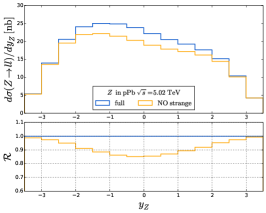
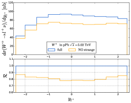
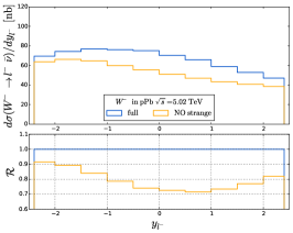
(a) $\sqrt{s}=5.02$ TeV

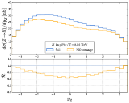
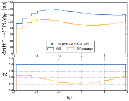
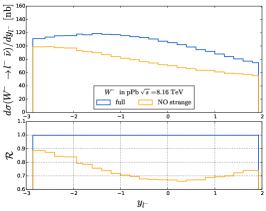
(b) $\sqrt{s}=8.16$ TeV

Figure 1: Contribution of strange initiated channels to $W^{\pm}$ and $Z$ boson production for proton-lead ($p$Pb) at the LHC. The blue lines represent total cross-sections, the yellow lines are cross-sections with the strange initiated channels subtracted. The lower panels show the ratio compared to the total cross-section.

Parton distribution functions (PDFs) are key elements required to generate concrete predictions for processes with hadronic initial states in the context of QCD factorization theorems. The success of this theoretical framework has been extensively demonstrated in fixed-target and collider experiments (e.g., at the TeVatron, SLAC, HERA, RHIC, LHC), and will be essential for making predictions for future facilities (EIC, LHeC, FCC). Despite the above achievements, there is yet much to learn about the hadronic structure and the detailed composition of the PDFs Hou:2019efy ; Ball:2017nwa ; Kovarik:2015cma ; Eskola:2016oht ; AbdulKhalek:2019mzd ; AbdulKhalek:2020yuc ; Ethier:2020way ; Khalek:2018mdn ; Gao:2017yyd ; Kovarik:2019xvh ; Alekhin:2017olj ; Hou:2019efy ; Nadolsky:2008zw ; Sato:2019yez ; Harland-Lang:2014zoa ; Thorne:2019mpt ; Ball:2009mk ; Lin:2017snn ; Lin:2020rut .

Although the up and down PDF flavors are generally well-determined across much of the partonic $x$ range, there is significant uncertainty in the strange component, $s(x)$. The strange PDF is especially challenging because, in many processes, it is difficult to separate it from the larger down component. However, as we push to higher precision and energies, an accurate determination of the strange PDF is, apart from its intrinsic fundamental importance, essential not only for LHC measurements, but for a wide variety of processes Alekhin:2017olj ; Hou:2019efy ; Nadolsky:2008zw ; Sato:2019yez ; Harland-Lang:2014zoa ; Thorne:2019mpt ; Ball:2009mk ; Lin:2017snn ; Lin:2020rut . For example, the knowledge of the nuclear strange distribution in heavy nuclei is crucial for providing a reliable baseline for hard probes of the quark gluon plasma (QGP) which is characterized by enhanced production of strangeness Rafelski:1982pu ; Deak:2017dgs ; Gale:2020xlg . Additionally, small $x$ nuclear PDFs are essential for computing the composition of air showers from ultra-high energy cosmic rays Bhattacharya:2016jce ; Reno:2019jtr ; Bai:2020ukz ; Zenaiev:2019ktw .

The recent results from the LHC for $W/Z$ boson production in $pp$ collisions predict a large strange to light-sea ratio Aad:2012sb ; Aad:2014xca ; Aaboud:2016btc ; ATLAS:2019ext ; Chatrchyan:2013uja ; Sirunyan:2018hde . This is a rather surprising result as it differs from earlier determinations based on analyses of neutrino deep inelastic scattering (DIS) data from NuTeV and CCFR experiments Tzanov:2005kr ; Mason:2007zz ; Goncharov:2001qe or charged kaon production data from HERMES Airapetian:2008qf . See Ref. Kusina:2012vh for more details on the earlier determinations of the strange distribution, and Ref. Cooper-Sarkar:2018ufj for a study of the compatibility of the ATLAS and CMS results using the xFitter framework Alekhin:2014irh .

It is not easy to directly compare the $pp$ LHC results with the fixed target experiments, as the earlier measurements were generally done using nuclear targets (typically Fe or Pb). Additional complications arise from the fact that there is a controversy about the proper nuclear correction factors for the charged current (CC) and neutral current (NC) DIS measurements Kovarik:2010uv ; Schienbein:2009kk ; Kalantarians:2017mkj ; Paukkunen:2013grz ; Paukkunen:2010hb . As a result, the choice of heavy target neutrino DIS data sets varies widely among not just the many nuclear PDF (nPDF) determinations, but also for the proton PDF fits Hou:2019efy ; Ball:2017nwa . Moreover, in the proton case the nuclear corrections are applied in different ways.

Conversely, it was already demonstrated that the $W/Z$ LHC data can provide some important information on the strange and gluon nPDFs Kusina:2016fxy ; Eskola:2016oht ; AbdulKhalek:2020yuc . To demonstrate the impact of the heavy ion $W^{\pm}\!/Z$  data on the strange PDF, in Fig. 1 we display the contribution of the strange-initiated process as a function of rapidity. We observe the strange component can be as much as 20% to 30% of the total. For this reason, we concentrate in the following on the constraints for the nuclear strange and gluon distributions given by the $W$ and $Z$ data from proton-lead ($p$Pb) collisions at the LHC. This process is an ideal QCD “laboratory” as it is sensitive to i) the heavy flavor components $\{s,c,...\}$, ii) the nuclear corrections, and iii) the underlying “base” proton PDFs. Such an analysis provides an independent perspective on the subject and can help disentangle the flavor separation and nuclear modifications.

In the current investigation, we will study the production of $W$ and $Z$ bosons in proton–lead ($p$Pb) collisions at the LHC; this involves similar considerations as the $pp$ case, but also brings in the nuclear corrections. We will be focusing, in particular, on the strange and gluon distributions to see how these are modified when the LHC measurements are included. In Sec. II we review the various data sets used in our analysis along with the separate fits extracted. In Sec. III we present the quality of the fits and comparisons of data with the theory, and demonstrate the impact on the resulting PDFs. In Sec. IV we compare our final PDF fit with other results from the literature. In Sec. V we recap the key outcomes of this study.

II Fits to Experimental Data

II.1 The nCTEQ++ Framework

The nCTEQ project extends the proton PDF global fitting effort by fully including the nuclear dimension. Previous to the nCTEQ effort, nuclear data was “corrected” to isoscalar data and added to the proton PDF fit without any uncertainties Olness:2003wz . In contrast, the nCTEQ framework allows full communication between the nuclear data and the proton data; this enables us to investigate if observed tensions between data sets could potentially be attributed to the nuclear corrections.

The details of the nCTEQ15 nPDFs are presented in Ref. Kovarik:2015cma . The present analysis is performed in a new C++ code base (nCTEQ++) which enabled us to easily interface to external programs such as HOPPET Salam:2008qg , APPLgrid Carli:2010rw , and MCFM Campbell:2015qma . The nCTEQ15 fit has been reproduced in this new nCTEQ++ framework.

For the current set of fits, we use the same 16 free parameters as for the nCTEQ15 set, and additionally open up three parameters for the strange PDF, for a total of 19 parameters. Recall that for the nCTEQ15 set, the strange PDF was constrained by the relation $s=\bar{s}=(\kappa/2)(\bar{u}+\bar{d})$ at the initial scale $Q_{0}=1.3$ GeV so that it had the same form as the sea quarks.

Our PDFs are parameterized as

$$xf_{i}^{p/A}(x,Q_{0})=c_{0}x^{c_{1}}(1-x)^{c_{2}}e^{c_{3}x}(1+e^{c_{4}}x)^{c_{5}}\quad,$$ (1)

and the nuclear $A$ dependence is encoded in the coefficients as

$$c_{k}\longrightarrow c_{k}(A)\equiv c_{k,0}+c_{k,1}(1-A^{-c_{k,2}})\quad,$$ (2)

where $k=\{1,...,5\}$.

The 16 free parameters used for the nCTEQ15 set model the $x$-dependence of the $\{g,u_{v},d_{v},\bar{d}+\bar{u}\}$ PDF combinations, and we do not vary the $\bar{d}/\bar{u}$ parameters; see Ref. Kovarik:2015cma for details. To this, we now add three strange PDF parameters: $\{c_{0,1}^{s+\bar{s}},c_{1,1}^{s+\bar{s}},c_{2,1}^{s+\bar{s}}\}$; these parameters describe, correspondingly, the overall normalization, the low-$x$ exponent and the large $x$ exponent of the strange distribution.

II.2 Experimental Data Sets

Data Overview
			$\sqrt{s_{NN}}$ [TeV]	Norm $\sigma$	No Points	Ref.
ATLAS	Run I	$W^{\pm}$	5.02	2.7%	10+10	AtlasWpPb
ATLAS	Run I	$Z$	5.02	2.7%	14	Aad:2015gta
CMS	Run I	$W^{\pm}$	5.02	3.5%	10+10	Khachatryan:2015hha
CMS	Run I	$Z$	5.02	3.5%	12	Khachatryan:2015pzs
CMS	Run II	$W^{\pm}$	8.16	3.5%	24+24	Sirunyan:2019dox
ALICE	Run I	$W^{\pm}$	5.02	2.0%	2+2	Alice:2016wka ; Senosi:2015omk
LHCb	Run I	$Z$	5.02	2.0%	2	Aaij:2014pvu

Table 1: The overview of the LHC $W^{\pm}/Z$ data sets including the $p$Pb system with per nucleon center-of-mass enery $\sqrt{s_{NN}}$, experimental normalization uncertainty of the data, number of data points, and references.

Normalization Shifts
	ATLAS Run I			CMS Run I			CMS Run II
	$W^{-}$	$W^{+}$	$Z$	$W^{-}$	$W^{+}$	$Z$	$W^{-}$	$W^{+}$
Set ID	6211	6213	6215	6231	6233	6235	6232	6234
Norm0	—			—			—
Norm2	0.963			0.949			—
Norm3	0.955			0.937			0.960

Table 2: The LHC $W^{\pm}\!/Z$ data sets and the corresponding ID’s are listed. The normalization factors (where appropriate) are applied to the data sets. The normalization shifts for the nCTEQ15WZ set are the same as for the Norm3 fit.

$\chi^{2}/N_{dof}$ for Selected Experiments & Processes
	ATLAS Run I			CMS Run I			CMS Run II		ALICE		LHCb		DIS	DY	Pion	LHC	LHC	Total
	$W^{-}$	$W^{+}$	$Z$	$W^{-}$	$W^{+}$	$Z$	$W^{-}$	$W^{+}$	$W^{-}$	$W^{+}$	$Z$						Norm $\chi^{2}$
nCTEQ15	1.38	0.71	2.88	6.13	6.38	0.05	9.65	13.20	2.30	1.46	0.70		0.91	0.73	0.25	6.20	—	1.66
Norm0	0.94	0.26	2.71	3.89	2.25	0.03	1.07	1.51	0.53	0.02	0.71		0.92	0.95	0.83	1.47	—	1.03
Norm2	0.78	0.37	1.90	1.60	1.02	0.21	1.25	1.59	0.59	0.02	0.68		0.93	0.87	0.61	1.15	13.2	0.98
Norm3	0.83	0.46	1.78	1.41	1.23	0.31	0.74	0.84	0.75	0.08	0.62		0.90	0.77	0.39	0.91	22.9	0.91
nCTEQ15WZ	0.84	0.46	1.79	1.43	1.22	0.31	0.72	0.80	0.80	0.11	0.62		0.90	0.78	0.38	0.90	22.9	0.91

Table 3: We present the $\chi^{2}/N_{dof}$ for the individual data sets, the individual processes {DIS, DY, Pion, LHC}, and the total. We also show the total $\chi^{2}$ contribution from the LHC normalization penalty. Note that the Pion $\chi^{2}/N_{dof}$ is shown for comparison, but this data is only included in the nCTEQ15WZ fit.

In this analysis we use the deep inelastic scattering (DIS), Drell-Yan (DY) lepton pair production, and RHIC pion data employed in our earlier nCTEQ15 analysis Kovarik:2015cma . Additionally, we use $W$ and $Z$ inclusive data from proton-lead collisions at the LHC. Specifically, we include the following data sets: ALICE $W^{\pm}$ boson production Alice:2016wka ; Senosi:2015omk , ATLAS $Z$ boson production Aad:2015gta , ATLAS $W^{\pm}$ boson production AtlasWpPb , CMS $Z$ boson production Khachatryan:2015pzs , CMS $W^{\pm}$ boson production Khachatryan:2015hha , CMS Run II $W^{\pm}$ boson production Sirunyan:2019dox , and LHCb $Z$ boson production Aaij:2014pvu . The data sets are outlined in Table 1. All the theory calculations are performed at the next-to-leading order (NLO) of QCD. In particular, the calculations for $W$ and $Z$ boson production have been performed using the MCFM-6.8 program Campbell:2011bn interfaced with APPLgrid Carli:2010rw in order to speed up the computations.

II.3 The PDF Fits

We now use the nCTEQ++ framework to include the LHC $W^{\pm}\!/Z$ $p$Pb data and extend the nCTEQ15 fit. Comparing the LHC $p$Pb data to the nCTEQ15 results, we find that these data generally lie above the theory predictions Kusina:2016fxy ; hence, if we allow for a normalization uncertainty, this additional freedom can significantly improve the fit. The experiments have an associated luminosity uncertainty (cf., Table 2), and we will use this as a gauge as we shift the data normalizations. It is reasonable to tie the normalizations for $\{W^{\pm},Z\}$ data from individual experiments (e.g, CMS Run I) to a single normalization factor as these uncertainties are fully correlated.

Previous studies implied a close connection between the normalization of the $W^{\pm}\!/Z$ data and the extracted strange PDF Kusina:2016fxy . To systematically investigate the effect of the normalization in detail, we will use a series of fits outlined in Table 3 and summarized below:

nCTEQ15

This is the original set of nuclear PDFs as computed in Ref. Kovarik:2015cma .

Norm0

We include the LHC $p$Pb data, but we do not allow for any floating normalization of the LHC data.

Norm2

We include the LHC $p$Pb data, and allow for 2 normalization factors; one for the ATLAS Run I data, one for CMS Run I; we do not renormalize CMS Run II data in this fit.

Norm3

We include the LHC $p$Pb data, and we allow for 3 normalization factors; one for the ATLAS Run I data, one for the CMS Run I data, and a separate one for the CMS Run II data.

nCTEQ15WZ

This is the same as Norm3, but we also include the RHIC inclusive pion data directly in the fit. This is discussed in Sec. IV.

All four of these new PDF fits are based on the DIS and DY data from the nCTEQ15 analysis and the LHC data sets, as outlined in Sec. II.2 and Table 1.

As with our nCTEQ15 study, we will present results both with and without the inclusive pion data Adler:2006wg ; Abelev:2009hx . For the comparison of the the $W^{\pm}\!/Z$ normalizations fits {Norm0, Norm2, Norm3}, we will not include the pion data; however, we do compute the pion $\chi^{2}$, as shown in Table 3, to demonstrate the compatibility.

In Sec. IV we then present a separate fit, nCTEQ15WZ, which does include the pion data. As we will see the impact of the pion data is marginal.

Normalization Factors: Table 2 shows the determined normalization factors used in each fit. All the normalization shifts are between $1\sigma$ and $2\sigma$ of the quoted normalization uncertainty, but all are systematically below unity; the appropriate normalization penalties are included in the $\chi^{2}$ calculations. The detailed prescription we use for fitting data normalizations is provided in the Appendix A. For the ALICE and LHCb sets, the current uncertainties provide sufficient flexibility that we do not use an additional normalization factor for these data.

III Results and Discussion

Having presented our series of fits, we now examine i) the quality of these fits as measured by the $\chi^{2}$ values, ii) the comparison of the data with our theory predictions, and iii) the impact on the underlying PDFs.

III.1 Quality of the fits

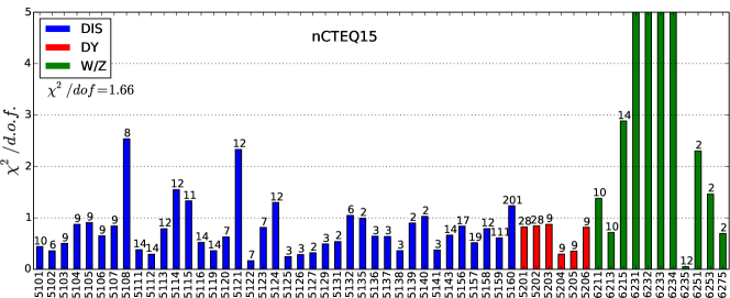
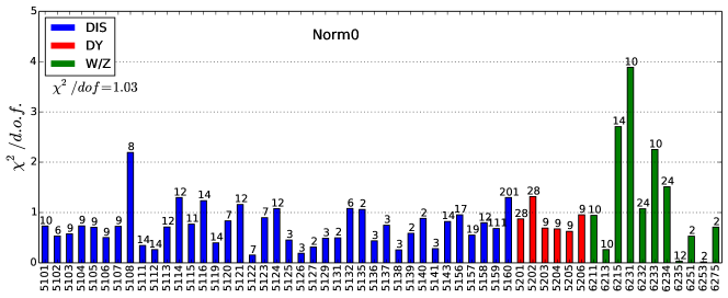
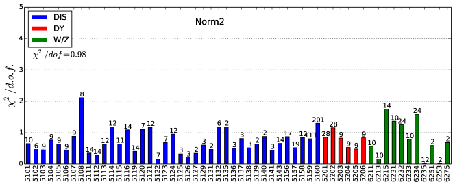
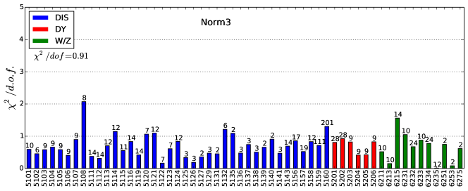
Figure 2: The $\chi^{2}/N_{dof}$ of the individual experiments. The number of data points is indicated at the top of the bar, and the total $\chi^{2}/N_{dof}$ for the entire set is shown below the legend. For the nCTEQ15 set, four of the bars extend beyond the chart range; these are $\chi^{2}/N_{dof}=\{6.1,9.7,6.4,13.2\}$ for experiments $\{6231,6232,6233,6234\}$.

Overall quality of the fits: In Tab. 3 we present the $\chi^{2}/N_{dof}$ for selected data sets as well as for each experiment type, and the contribution of the normalization penalty to the total $\chi^{2}/N_{dof}$. We compute the normalization penalty as outlined in Appendix A, and this is included in the total.

Examining the total $\chi^{2}/N_{dof}$ of the fits, we see a broad range spanning from 1.66 for nCTEQ15 to values below 1.00, and an even larger range of the $\chi^{2}/N_{dof}$ for the individual LHC data sets.

Quality of individual data sets: To provide more details regarding the source of the $\chi^{2}$ contributions, in Fig. 2 we display the $\chi^{2}/N_{dof}$ values for each individual experiment which enters the fit. The experiments are identified by their 4-digit ID, and the number of data points is indicated at the top of each bar. Additionally, the bars are color-coded to indicate the type of observable {DIS, DY,W/Z}.

The $\chi^{2}/N_{dof}$ bar charts provide incisive information as to which data sets are driving the fit. We discuss each fit in turn.

nCTEQ15: Starting with the nCTEQ15 set, we note that (except for a few outliers) the DIS and DY data is well described by these PDFs; by comparison, the LHC $W^{\pm}/Z$ data (which was not included in the original nCTEQ15 fit) is not well described. As was detailed in Ref. Kusina:2016fxy , an important contribution to this large $\chi^{2}$ comes from the small $x$ region where the nuclear PDFs are poorly constrained. The re-weighting analysis of Ref. Kusina:2016fxy demonstrated that we can improve the fit by adjusting the small $x$ behavior of the PDFs, but this alone will not bring all the data sets into the range of $\chi^{2}/N_{dof}\sim 1$; something else is required.

Norm0: As a first step, this fit includes the LHC $W^{\pm}/Z$ data, but does not include any floating normalization factors. This fit will tell us the extent to which we can adjust the PDFs to fit the LHC data before we begin to adjust the normalization factors. Examining Fig. 2, we see the impact of this fit on the DIS and DY data is generally small for many of the data sets, but does result in noticeable improvement for a few of the sets including 5115 (NMC Ca/D) and 5121 (NMC Li/D), for example. However, it does significantly improve the LHC $W^{\pm}/Z$ fit reducing the partial $\chi^{2}/N_{dof}$ of this data from 6.20 to 1.47 for the 120 LHC data points. Although this is a notable improvement, a number of the LHC data sets still have $\chi^{2}/N_{dof}$ values well above one.

Norm2: In this fit, we allow two floating normalization factors (one for ATLAS and one for CMS Run I) which are allowed to vary in the fit. The contribution of the normalization penalty is included in the total $\chi^{2}$.

We see the impact of the floating normalization factors on the DIS and DY data is again small, as was the case for the Norm0 fit. But the Norm2 fit dramatically improves the LHC $W^{\pm}/Z$ data reducing $\chi^{2}/N_{dof}$ of this data to 1.15 as compared to 1.47 for the Norm0 fit. While the Norm2 fit is a substantial improvement over the Norm0 results and all LHC data sets have $\chi^{2}/N_{dof}<2$, there are still a few sets at the upper limit of this range.

Norm3: Finally, we now perform a fit with three normalization factors: one for ATLAS (Run I), and one for each CMS Run I and CMS Run II.

As before, the modifications to the DIS and DY sets are minimal, but we do continue to see an improvement in the LHC sets; namely the $\chi^{2}/N_{dof}$ of this data improves to 0.91 as compared to 1.15 for the Norm2 fit.

Comparing Norm3 with nCTEQ15 for the other data sets, we see that the $\chi^{2}/N_{dof}$ for the DIS data is essentially the same (0.91 vs. 0.90), the DY increases slightly (0.73 vs. 0.77), and the pion $\chi^{2}$ (computed a posteriori) increases slightly as well (0.25 vs. 0.39); these differences are relatively small compared to the significant improvement in the LHC data (6.20 vs. 0.90).

III.2 Comparison of Data with Theory

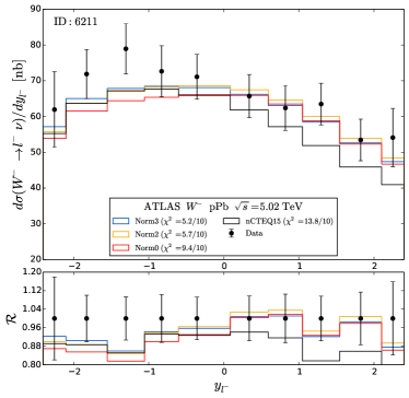
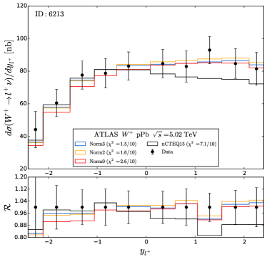
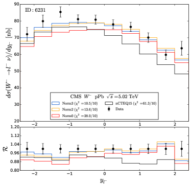
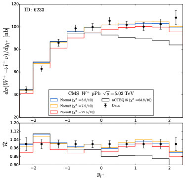
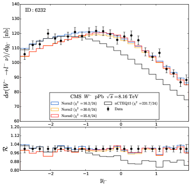
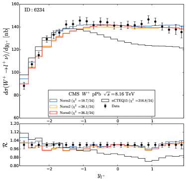
Figure 3: Comparison of data with theory for ATLAS and CMS $W^{\pm}$ production. The normalization shifts are applied to the theory so we can compare all the results on a single plot; the data is unaltered. For reference, ATLAS Run I $\{W^{-},W^{+}\}=\{6211,6213\}$, CMS Run I $\{W^{-},W^{+}\}=\{6231,6233\}$ and CMS Run I $\{W^{-},W^{+}\}=\{6232,6234\}$.

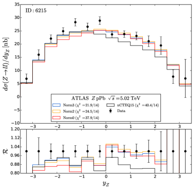
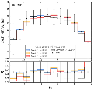
Figure 4: Comparison of data with theory for ATLAS and CMS $Z$ production. The normalization shifts are applied to the theory so we can compare all the results on a single plot; the data is unaltered. For reference, ATLAS Run I $\{Z\}=\{6215\}$ and CMS Run I $\{Z\}=\{6235\}$.

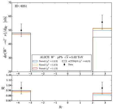
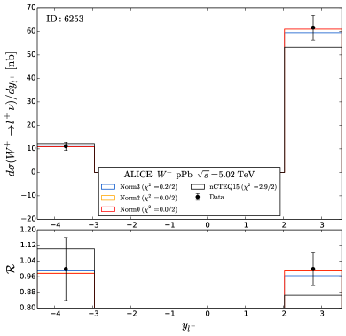
Figure 5: Comparison of data with theory for ALICE $W^{\pm}$ production. The normalization shifts are applied to the theory so we can compare all the results on a single plot; the data is unaltered. For reference, ALICE Run I $\{W^{-},W^{+}\}=\{6251,6253\}$.

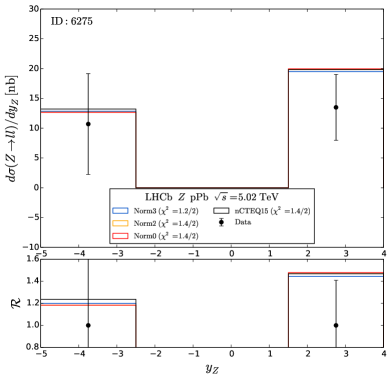
Figure 6: Comparison of data with theory for LHCb $Z$ production (ID 6275). The normalization shifts are applied to the theory so we can compare all the results on a single plot; the data is unaltered.

To obtain a more complete view of the fit quality, in Figs. 3, 4, 5, and 6 we display the comparison of the LHC data with theory predictions. The data points and errors are taken directly from the experimental measurements. However, it is important to note that we have shifted the theoretical predictions by the appropriate normalization factors; this allows us to present the fits with different normalizations on a single plot, and provides a more accurate visual description of the quality of the fit.

III.2.1 Large $x$ Region:

Our first observation is that the experimental data consistently lies above our theoretical predictions. From Table 2, recall that all the fitted normalization factors are less than one, indicating that the fit prefers a reduction of the data values, typically in the range of $\sim 5\%$; because we have shifted the theory, this is not as obvious in Figs. 3–6.

Even with the normalization shifts, we see the theory predictions still lie well below the data for a number of sets. This is most evident in the negative $y$ region for the Run I $W^{-}$ data sets 6211 (ATLAS $W^{-}$) and 6231 (CMS $W^{-}$ Run I), and to a lesser extent 6215 (ATLAS $Z$). Interestingly, the Run II data generally show good agreement across the full $y$ range.

The negative rapidity region corresponds to the large $x$ region of the lead PDF. The large $x$ region is already rather well constrained by the fixed-target measurements, so there are limits as to how much the new LHC data can shift the PDFs in this region. Also note, that in the large $x$ region we are in the “anti-shadowing region” ($x\sim 0.1$) where the nuclear corrections typically enhance the nuclear PDF relative to the proton. Thus, not including the nuclear corrections in this region would increase the discrepancy.

III.2.2 Small $x$ Region:

In the large rapidity (small $x$) region, we generally find good agreement between our new fits and the data. But, this is in striking contrast to the nCTEQ15 PDF which lies well below many of the data points at large $y$; this behavior is clearly evident, for example, in 6215 (ATLAS $Z$), and 6213, 6232, 6233, 6234 (CMS $W^{\pm}$ Run I and Run II). Clearly, the new LHC $W^{\pm}\!/Z$ data provides important new PDF constraints in this kinematic region that were not available in the nCTEQ15 analysis.

As larger rapidity corresponds to smaller $x$ values, this puts us in the “shadowing region” ($x\lesssim 0.1$) where the nuclear PDFs are generally expected to be suppressed relative to the proton. If the nuclear shadowing correction were reduced in this region, that would bring the theory closer in line with the data without the need for large normalization factors. The precise value of the nuclear corrections is still an open question; for example, Refs. Schienbein:2009kk ; Kovarik:2010uv ; Owens:2007kp found that the shadowing correction for the $\nu N$ charged-current neutrino DIS was reduced as compared to the $\ell^{\pm}N$ neutral-current DIS. If such an adjustment were applied to the LHC $W^{\pm}\!/Z$ data, it would move the theory closer to the data and reduce the normalization factor. Disentangling the nuclear effects from the underlying parton flavor components is intricate, and a reanalysis of the neutrino DIS data is currently in progress ncteqNeutrino .

III.3 The PDFs

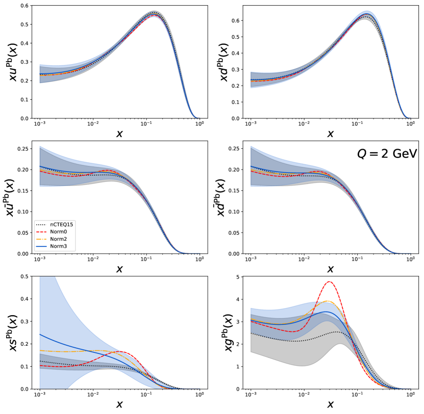
Figure 7: The full lead (Pb) PDFs for $Q=2$ GeV. The uncertainty band for nCTEQ15 is shown in gray, and for Norm3 in blue. The increase of the Norm0 set is evident for the strange and gluon PDFs in the region of $x\sim 0.03$.

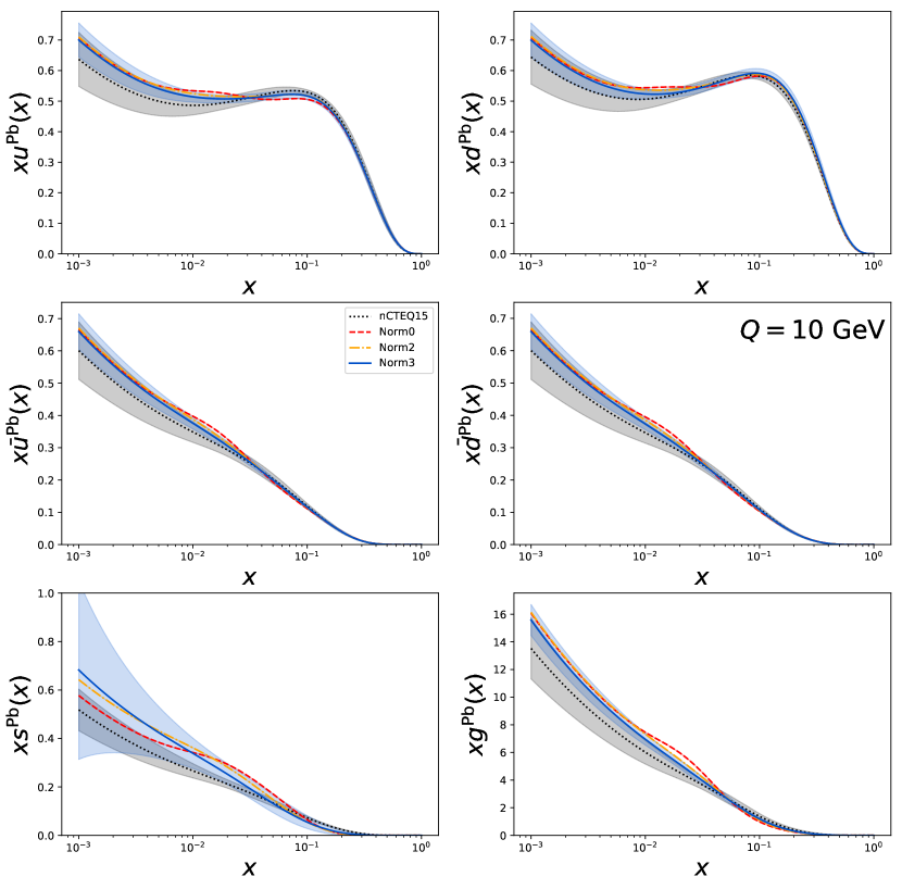
Figure 8: The full lead (Pb) PDFs for $Q=10$ GeV. The uncertainty band for nCTEQ15 is shown in gray, and for Norm3 in blue. The increase in the Norm0 set for the strange and gluon PDFs is reduced, compared to the lower $Q$ result, and shifted to smaller $x\sim 0.02$ values.

Figure 9: The full lead (Pb) PDFs for $Q=90$ GeV. The uncertainty band for nCTEQ15 is shown in gray, and for Norm3 in blue.

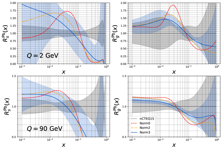
Figure 10: Ratio of strange and gluon nPDFs compared to the corresponding nCTEQ15 nPDFs for $Q=2$ GeV (upper row) and $Q=90$ GeV (lower row). The uncertainty band for nCTEQ15 is shown in gray, and for Norm3 in blue.

Finally, we make a detailed examination of the underlying flavor PDFs from these various fits. In Figs. 7–9 we display the nPDFs for a full lead nucleus at three separate scales. The lowest scale ($Q=2$ GeV) is close to our initial evolution scale of $Q_{0}=1.3$ GeV, the largest scale ($Q=90$ GeV) is in the range relevant for $W^{\pm}/Z$ production, and the intermediate scale ($Q=10$ GeV) helps illustrate the effects of the DGLAP evolution.

We choose to display the full lead nPDF as this is the physical quantity which enters the calculation. This is computed using:

$$f_{i}^{(A,Z)}(x,Q)=\frac{Z}{A}f_{i}^{p/A}(x,Q)+\frac{A-Z}{A}f_{i}^{n/A}(x,Q)\quad,$$ (3)

and we assume isospin symmetry to derive the neutron PDF.

III.3.1 Strange and Gluon nPDFs:

Examining the curves for up and down distributions, we see there is minimal variation between different fits as these flavors are strongly constrained by other data. Interestingly, we also see that the small $x$ uncertainty is reduced at higher scales (see Figs. 8 and 9). We observe a slight modification in the $\bar{u}$ and $\bar{d}$ distributions as these are closely linked to the gluon and strange distributions which we will discuss in the following.

Turning to the gluon and strange PDFs, we see significant differences. In particular, the fits seems to prefer a larger value for both the gluon and strange PDFs at intermediate $x$ values, which is the region relevant for the LHC heavy ion $W^{\pm}/Z$ production. We discuss these fits in turn.

Norm0: Examining the Norm0 fit for $Q=2$ GeV (Fig. 7), we see a distinct excess in the strange and gluon PDFs in the region $x\sim 0.03$; this is also evident in Fig. 10 where we have plotted the ratio relative to the nCTEQ15 values. At $Q=2$ GeV, the peak of the gluon and strange distributions are located at approximately $x\sim 0.03$; via the DGLAP evolution these peaks shift down to the region $x\sim 0.017$ for $Q=90$ GeV, consistent with the expectation for the central $x$ value of $\sim M_{W,Z}/\sqrt{s}$.

Recall that the Norm0 fit does not allow any normalization adjustment in the fit. Since the data consistently lie above the theoretical predictions, it appears that the Norm0 fit is exploiting the uncertainty of gluon and strange PDFs to try and pull up the theoretical predictions in line with the data by increasing the PDFs in the relevant $x$ region. Additionally, we observe a similar (but less pronounced) behavior in the $\bar{u}$ and $\bar{d}$ distributions.

As momentum must be conserved, we see the Norm0 strange PDF dips below nCTEQ15 at both high and low $x$ values, while the gluon is below nCTEQ15 at higher $x$ values. Part of the reason the deformation of the gluon and strange PDFs is so large at $Q=2$ GeV is to compensate for the DGLAP evolution which will tend to diffuse the excess in the gluon and strange distributions at the $Q=90$ GeV scale, cf., Fig. 9.

Norm2 and Norm3: In contrast to the Norm0 result above, the Norm2 and Norm3 fits allow us to investigate the effect of including the normalization parameters into the fit; this is crucial in reducing the $\chi^{2}/N_{dof}$ for the LHC heavy ion data. The effect on the resulting nPDFs is evident as shown in Fig. 7 where we see that the excess in both the strange and gluon is systematically reduced as we introduce normalization parameters.

In Fig. 7 we also observe the greatly increased error band on the Norm3 strange PDF as compared to nCTEQ15; this is of course due to the additional fitting parameters for the strange quark included in the Norm3 analysis.

To highlight the magnitude of these differences, in Fig. 10 we plot the ratios of the PDFs compared to nCTEQ15. At $Q=2$ GeV, we see that the Norm0 gluon is nearly a factor of 2 times the nCTEQ15 value, with a peak at $x\sim 0.03$. The Norm2 and Norm3 gluon PDFs are reduced to $\sim 60\%$ and $\sim 40\%$ above nCTEQ15, respectively. Similarly, at $x\sim 0.03$ and $Q=2$ GeV, the strange PDF for both Norm0 and Norm2 are $\sim 60\%$ above the nCTEQ15 value, while the Norm3 result is reduced to $\sim 25\%$.

In Fig. 10 we also display ratio at $Q=90$ GeV which illustrates the effect of the DGLAP evolution. We see that the gluon is now reduced to $\sim 15\%$ above the nCTEQ15 value, the strange is reduced to $\sim 25\%$ above the nCTEQ15 value, and both peaks have shifted to lower $x$ values.

Because the DGLAP evolution has “washed out” the detailed peak structure at low $Q$ values, it is necessary for the fit to amplify the distortion at low $Q$ so that a remnant of the effect survives at high $Q$. Nevertheless, the remaining excess at $Q=90$ GeV is sufficient to improve the $\chi^{2}$ of the fits.

Additionally, we note that the heavy-flavor reweighting analysis of Ref. Kusina:2017gkz also observed an increase of the gluon nPDF in the intermediate to small $x$ region relative to the nCTEQ15 results. While the shift of the PDF in the reweighting was in the same direction as in this analysis, its magnitude was much smaller.

We now turn our attention to the error band of the gluon distribution in Fig. 10. At NLO, the gluon enters for the first time the $W^{\pm}$ and $Z$ boson production through the $gq$ initiated contributions. The addition of the $W^{\pm}/Z$ LHC data to the fit is thus not expected to add significant constraining power for the gluon distribution. Contrary to this naive expectation, due to high center of mass energy and relatively small values of the probed $x$, the gluon distribution can have a considerable contribution to $W^{\pm}/Z$ production processes; this is reflected in the reduced error bands of Norm3 as compared with nCTEQ15. Indeed, an independent variation of the open gluon parameters around the minimum in the Norm3 fit confirms that the $\chi^{2}$ contribution from the LHC data is similarly steep or steeper than contribution from all the other data included in the fit.

IV Comparisons

IV.1 Comparison with other nPDFs

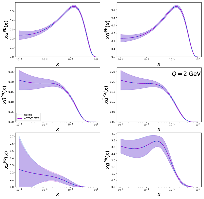
Figure 11: Comparison of the full lead (Pb) PDFs at $Q=2$ GeV for nCTEQ15WZ and Norm3 fits. The uncertainty band for nCTEQ15WZ is shown in purple, Norm3 in blue. This shows that the central value of these fits are essentially identical, and the error bands are also virtually identical with the exception of small differences in the strange quark PDF.

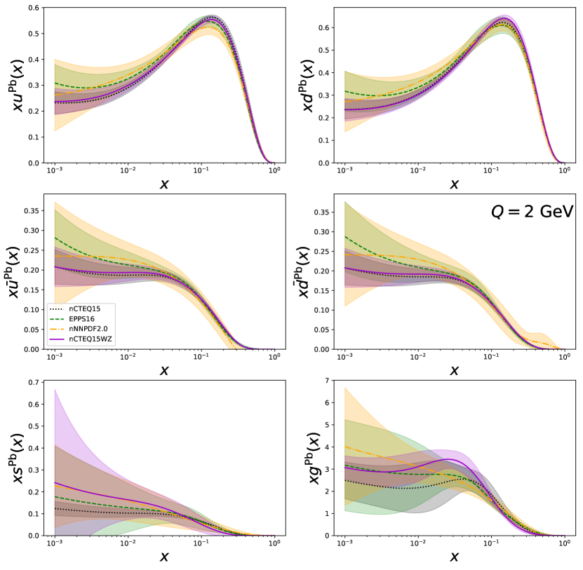
Figure 12: Comparison of the full lead (Pb) PDFs at $Q=2$ GeV for nCTEQ15, EPPS16, nNNPDF2.0 and nCTEQ15WZ. The uncertainty band for nCTEQ15 is shown in gray, nCTEQ15WZ in violet, nNNPDF2.0 in yellow and EPPS16 in green.

Figure 13: Comparison of the full lead (Pb) PDFs at $Q=90$ GeV for nCTEQ15, EPPS16, nNNPDF2.0 and nCTEQ15WZ. The uncertainty band for nCTEQ15 is shown in gray, nCTEQ15WZ in violet, nNNPDF2.0 in yellow and EPPS16 in green.

Having investigated the impact of the $W^{\pm}\!/Z$ heavy ion data including normalization effects, we now compare our PDFs with other results from the literature.

There are a number of nPDF sets available Hirai:2007sx ; Eskola:2009uj ; deFlorian:2011fp including some new determinations Walt:2019slu ; AbdulKhalek:2019mzd ; AbdulKhalek:2020yuc . The TUJU19 analysis Walt:2019slu extends the xFitter framework to include nuclear PDFs; this open-source program provides a valuable tool for the PDF community. As an initial step, TUJU19 assumed $s=\bar{s}$ and $s=\bar{u}=\bar{d}$, and the resulting nPDFs compare favorably with EPPS16 and nCTEQ15 within uncertainties.

A separate effort by the NNPDF collaboration AbdulKhalek:2019mzd ; AbdulKhalek:2020yuc uses neural network techniques to extract the gluon and quark nPDFs; this method provides a complementary approach to the traditional parameterized function-based method. Their recent analysis AbdulKhalek:2020yuc has produced the nNNPDF2.0 nPDF set which includes charged current DIS data from NuTeV (Fe) and Chorus (Pb), and also LHC $W^{\pm}\!/Z$ data. They also compute the strangeness ratio, $R_{s}=(s+\bar{s})/(\bar{u}+\bar{d})$, and find the nuclear value is reduced as compared to the proton. The neutrino DIS data and LHC $W+c$ associated production seem to prefer a lower $R_{s}$ value, while the inclusive $W$ and $Z$ production favor a larger value. These interesting observations raise some important issues, and additional investigation is warranted to better understand the strange distribution Ethier:2020way .

The EPPS16 data sets include DIS, DY, RHIC inclusive pion, and LHC $W^{\pm}\!/Z$ and dijet data; in particular, this set incorporates a number of parameters to provide flexibility in both the strange and gluon PDFs. Therefore, it will be interesting to compare the variation of these flavors between our original nCTEQ15 nPDFs and our nCTEQ15WZ fit.

The nCTEQ15WZ fit is based on the Norm3 fit (with 3 normalization parameters), and in addition includes the RHIC pion data in the fitting loop. The RHIC pion data is fit with the Binnewies-Kniehl-Kramer (BKK) fragmentation functions Binnewies:1994ju using a custom griding technique for fast evaluation Kovarik:2015cma . The resulting nCTEQ15WZ nPDFs are nearly identical as the Norm3 nPDFs which is evident when comparing the $\chi^{2}/N_{dof}$ values of Table 3, as well as the PDFs in Fig. 11.

We now compare the results of our nCTEQ15WZ fit with the nCTEQ15, EPPS16, and nNNPDF2.0 nPDFs in Figs. 12 and 13. To begin, we focus on the plots at $Q=2$ GeV as the variations are more evident here. For the up and down components $\{u,d,\bar{u},\bar{d}\}$, nCTEQ15WZ is quite similar to nCTEQ15, and these flavors generally lie below EPPS16 and nNNPDF2.0, but are within uncertainties. For the strange and gluon, we see that nCTEQ15 and EPPS16 are generally similar for larger $x$ values, and then diverge somewhat for small $x$. The nCTEQ15WZ nPDFs lie below nCTEQ15 and EPPS16 for large $x$ values, and then above at intermediate to small $x$ values; this allows $s(x)$ and $g(x)$ to increase the $W^{\pm}\!/Z$ cross section in the region of the data ($x\sim 0.02$) while not perturbing the momentum sum rules. nNNPDF2.0 is similar to nCTEQ15 and EPPS16 for large $x$ values, but then increases for smaller $x$. For the strange distribution, nNNPDF2.0 coincides with nCTEQ15WZ at small $x$, while for the gluon, nNNPDF2.0 exceeds nCTEQ15WZ at small $x$. Similar effects to the above are generally evident at larger $Q$ values (Fig. 13), but their magnitude is diminished due to the DGLAP evolution effects.

IV.2 Comparison with proton results

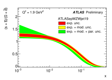
(a)

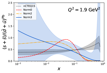
(b)

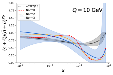
(c)

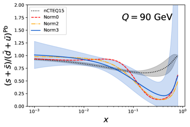
(d)

Figure 14: (a) Recent (preliminary) result from ATLAS on the strange ratio for the proton ATL-PHYS-PUB-2019-016 .  (b) The nuclear strange ratio for lead (Pb) nPDFs as obtained in our fits. The uncertainty band for nCTEQ15 is shown in gray, and Norm3 in blue.

The strange quark PDF has also been studied extensively for the proton case by many groups including ABM Alekhin:2017olj , CT18 Hou:2019efy , JAM Sato:2019yez , MMHT Harland-Lang:2014zoa ; Thorne:2019mpt , and NNPDF Ball:2009mk . There is a close connection between the proton and nuclear PDFs; for example, nCTEQ15 uses the proton PDF as a boundary condition, and EPPS16 fits nuclear ratios relative to the proton.

One quantity of interest we can compare between the proton and the nuclear PDFs is the ratio of the strange PDF relative to the light-sea quarks: $R_{s}={(s+\bar{s})/(\bar{u}+\bar{d})}$. In Fig. 14, we compute $R_{s}$ for selected $Q$ values, and compare this to the proton result as extracted by ATLAS ATLAS:2019ext ; Giuli:2019wtu .

Comparing the proton and the lead results at $Q^{2}=1.9~{}{\rm GeV}^{2}$, we see that the behavior of the Norm3 curve (panel-b) is quite similar to the proton result (panel-a). In contrast, the nCTEQ15 result is generally flat across all $x$ values as the strange was set to be a fixed fraction of the $u/d$-sea PDFs, $s=\bar{s}=\kappa(\bar{u}+\bar{d})/2$. Additionally, we also display the other fits, Norm0 and Norm2, to illustrate the range of possible variations. The uncertainty bands for Norm3 are displayed; these are large for small $x$, where the strange is poorly constrained, and also at very large $x$ where the quark sea denominator vanishes. We also display larger $Q$ values which illustrates the convergent effects of the DGLAP evolution.

In the previous section we raised the question as to whether the enhanced strange distribution was reflecting the true underlying physics, or was instead an artifact of the fit. The similarities of $R_{s}$ between the proton and lead PDFs may indicate that the enhanced strange PDF is, in fact, a real effect. To definitively answer this question will require additional analysis, and this work is ongoing.

V Conclusion

Our ability to fully characterize fundamental observables, like the Higgs boson couplings and the $W$ boson mass, and to constrain both SM and BSM signatures is strongly limited by how accurately we determine the underlying PDFs Tanabashi:2018oca . A precise determination of the strange PDF is an important step in advancing these measurements.

The new nCTEQ++ framework allowed us to include the LHC $W/Z$ data directly in the fit. While these new fits significantly reduced the overall $\chi^{2}$ for the $W/Z$ LHC data, we still observe tensions in individual data sets which require further investigation. Our analysis has identified factors which might further reduce the apparent discrepancies including: increasing the strange PDF, modifying the nuclear correction, and adjusting the data normalization.

Compared to the nCTEQ15 PDFs, these new fits favor an increased strange and gluon distribution in the $x$ region relevant for heavy ion $W^{\pm}\!/Z$ production. While we obtain a good fit in terms of the overall $\chi^{2}$ values, we must ask: i) how the uncertainties and data normalization affect the resulting PDFs, and ii) whether the results truly reflect the underlying physics, or is the fit simply exploiting $s(x)$ because that is one of the least constrained flavors? The answer to this important question will require additional study; this is currently under investigation.

Appendix A Fitting data normalizations

When fitting the normalization of data sets, we use the $\chi^{2}$ prescription given in Ref. DAgostini:1993arp . For a data set $D$ with $N$ data points and $S$ correlated systematic errors, the $\chi^{2}$ of the data set reads:

$$\chi^{2}_{D} = \sum_{i,j}^{N}\left(D_{i}-\frac{T_{i}}{N_{norm}}\right)(C^{-1})_{ij}\left(D_{j}-\frac{T_{j}}{N_{norm}}\right)$$ (4)

$$\qquad+\left(\frac{1-N_{norm}}{\sigma_{norm}}\right)^{2}$$

where $\sigma_{norm}$ is the normalization uncertainty and $T_{i}$ is the theoretical prediction for point $i$. The last term of Eq.(4) is called the normalization penalty and it enters when the fitted normalization, $N_{norm}$, differs from unity. The normalization uncertainty $\sigma_{norm}$ appearing in the denominator prevents large excursions of $N_{norm}$ away from unity.

The covariance matrix $C_{ij}$ is defined as:

$$C_{ij}=\sigma_{i}^{2}\,\delta_{ij}+\sum_{\alpha}^{S}\bar{\sigma}_{i\alpha}\,\bar{\sigma}_{j\beta}$$ (5)

where $\sigma_{i}$ is the total uncorrelated uncertainty (added in quadrature) for data point $i$, and $\bar{\sigma}_{i\alpha}$ is the correlated systematic uncertainty for data point $i$ from source $\alpha$. Using the analytical formula for the inverse of the correlation matrix as in Ref. Stump:2001gu , we obtain:

$$\chi^{2}_{D}=\sum_{i}\left(\frac{D_{i}-T_{i}/N_{norm}}{\sigma_{i}}\right)^{2}-B^{T}A^{-1}B+\left(\frac{1-N_{norm}}{\sigma_{norm}}\right)^{2},$$ (6)

with

$$A_{\alpha\gamma}=\delta_{\alpha\gamma}+\sum_{i}\frac{\bar{\sigma}_{i\alpha}\,\bar{\sigma}_{i\gamma}}{\sigma_{i}^{2}},$$ (7)

and

$$B_{\alpha}=\sum_{i}\frac{\bar{\sigma}_{i\alpha}\,(D_{i}-T_{i}/N_{norm})}{\sigma_{i}^{2}}.$$ (8)

References

- (1) T.-J. Hou et al., “New CTEQ global analysis of quantum chromodynamics with high-precision data from the LHC,” arXiv:1912.10053 [hep-ph].
- (2) NNPDF Collaboration, R. D. Ball et al., “Parton distributions from high-precision collider data,” Eur. Phys. J. C77 no. 10, (2017) 663, arXiv:1706.00428 [hep-ph].
- (3) K. Kovarik et al., “nCTEQ15 - Global analysis of nuclear parton distributions with uncertainties in the CTEQ framework,” Phys. Rev. D93 no. 8, (2016) 085037, arXiv:1509.00792 [hep-ph].
- (4) K. J. Eskola, P. Paakkinen, H. Paukkunen, and C. A. Salgado, “EPPS16: Nuclear parton distributions with LHC data,” Eur. Phys. J. C77 no. 3, (2017) 163, arXiv:1612.05741 [hep-ph].
- (5) NNPDF Collaboration, R. Abdul Khalek, J. J. Ethier, and J. Rojo, “Nuclear parton distributions from lepton-nucleus scattering and the impact of an electron-ion collider,” Eur. Phys. J. C79 no. 6, (2019) 471, arXiv:1904.00018 [hep-ph].
- (6) R. Abdul Khalek, J. J. Ethier, J. Rojo, and G. van Weelden, “nNNPDF2.0: Quark Flavor Separation in Nuclei from LHC Data,” arXiv:2006.14629 [hep-ph].
- (7) J. J. Ethier and E. R. Nocera, “Parton Distributions in Nucleons and Nuclei,” Ann. Rev. Nucl. Part. Sci. no. 70, (2020) 1–34, arXiv:2001.07722 [hep-ph].
- (8) R. Abdul Khalek, S. Bailey, J. Gao, L. Harland-Lang, and J. Rojo, “Towards Ultimate Parton Distributions at the High-Luminosity LHC,” Eur. Phys. J. C 78 no. 11, (2018) 962, arXiv:1810.03639 [hep-ph].
- (9) J. Gao, L. Harland-Lang, and J. Rojo, “The Structure of the Proton in the LHC Precision Era,” Phys. Rept. 742 (2018) 1–121, arXiv:1709.04922 [hep-ph].
- (10) K. Kovaˇrík, P. M. Nadolsky, and D. E. Soper, “Hadron structure in high-energy collisions,” arXiv:1905.06957 [hep-ph].
- (11) S. Alekhin, J. Blümlein, and S. Moch, “Strange sea determination from collider data,” Phys. Lett. B 777 (2018) 134–140, arXiv:1708.01067 [hep-ph].
- (12) P. M. Nadolsky, H.-L. Lai, Q.-H. Cao, J. Huston, J. Pumplin, D. Stump, W.-K. Tung, and C.-P. Yuan, “Implications of CTEQ global analysis for collider observables,” Phys. Rev. D 78 (2008) 013004, arXiv:0802.0007 [hep-ph].
- (13) JAM Collaboration, N. Sato, C. Andres, J. Ethier, and W. Melnitchouk, “Strange quark suppression from a simultaneous Monte Carlo analysis of parton distributions and fragmentation functions,” Phys. Rev. D 101 no. 7, (2020) 074020, arXiv:1905.03788 [hep-ph].
- (14) L. Harland-Lang, A. Martin, P. Motylinski, and R. Thorne, “Parton distributions in the LHC era: MMHT 2014 PDFs,” Eur. Phys. J. C 75 no. 5, (2015) 204, arXiv:1412.3989 [hep-ph].
- (15) R. S. Thorne, S. Bailey, T. Cridge, L. A. Harland-Lang, A. Martin, and R. Nathvani, “Updates of PDFs using the MMHT framework,” PoS DIS2019 (2019) 036, arXiv:1907.08147 [hep-ph].
- (16) NNPDF Collaboration, R. D. Ball, L. Del Debbio, S. Forte, A. Guffanti, J. I. Latorre, A. Piccione, J. Rojo, and M. Ubiali, “Precision determination of electroweak parameters and the strange content of the proton from neutrino deep-inelastic scattering,” Nucl. Phys. B 823 (2009) 195–233, arXiv:0906.1958 [hep-ph].
- (17) H.-W. Lin et al., “Parton distributions and lattice QCD calculations: a community white paper,” Prog. Part. Nucl. Phys. 100 (2018) 107–160, arXiv:1711.07916 [hep-ph].
- (18) H.-W. Lin et al., “Parton distributions and lattice QCD calculations: toward 3D structure,” arXiv:2006.08636 [hep-ph].
- (19) J. Rafelski and B. Muller, “Strangeness Production in the Quark - Gluon Plasma,” Phys. Rev. Lett. 48 (1982) 1066. [Erratum: Phys. Rev. Lett.56,2334(1986)].
- (20) M. Deák, K. Kutak, and K. Tywoniuk, “Towards tomography of quark–gluon plasma using double inclusive forward-central jets in Pb–Pb collision,” Eur. Phys. J. C 77 no. 11, (2017) 793, arXiv:1706.08434 [hep-ph].
- (21) C. Gale, J.-F. Paquet, B. Schenke, and C. Shen, “Probing Early-Time Dynamics and Quark-Gluon Plasma Transport Properties with Photons and Hadrons,” in 28th International Conference on Ultrarelativistic Nucleus-Nucleus Collisions. 2, 2020. arXiv:2002.05191 [hep-ph].
- (22) A. Bhattacharya, R. Enberg, Y. S. Jeong, C. Kim, M. H. Reno, I. Sarcevic, and A. Stasto, “Prompt atmospheric neutrino fluxes: perturbative QCD models and nuclear effects,” JHEP 11 (2016) 167, arXiv:1607.00193 [hep-ph].
- (23) M. H. Reno, J. F. Krizmanic, and T. M. Venters, “Cosmic tau neutrino detection via Cherenkov signals from air showers from Earth-emerging taus,” Phys. Rev. D 100 no. 6, (2019) 063010, arXiv:1902.11287 [astro-ph.HE].
- (24) W. Bai, M. Diwan, M. V. Garzelli, Y. S. Jeong, and M. H. Reno, “Far-forward neutrinos at the Large Hadron Collider,” JHEP 06 (2020) 032, arXiv:2002.03012 [hep-ph].
- (25) PROSA Collaboration, O. Zenaiev, M. Garzelli, K. Lipka, S. Moch, A. Cooper-Sarkar, F. Olness, A. Geiser, and G. Sigl, “Improved constraints on parton distributions using LHCb, ALICE and HERA heavy-flavour measurements and implications for the predictions for prompt atmospheric-neutrino fluxes,” JHEP 04 (2020) 118, arXiv:1911.13164 [hep-ph].
- (26) ATLAS Collaboration, G. Aad et al., “Determination of the strange quark density of the proton from ATLAS measurements of the and cross sections,” Phys. Rev. Lett. 109 (2012) 012001, arXiv:1203.4051 [hep-ex].
- (27) ATLAS Collaboration, G. Aad et al., “Measurement of the production of a boson in association with a charm quark in collisions at 7 TeV with the ATLAS detector,” JHEP 05 (2014) 068, arXiv:1402.6263 [hep-ex].
- (28) ATLAS Collaboration, M. Aaboud et al., “Precision measurement and interpretation of inclusive , and production cross sections with the ATLAS detector,” Eur. Phys. J. C77 no. 6, (2017) 367, arXiv:1612.03016 [hep-ex].
- (29) ATLAS Collaboration, T. A. collaboration, “QCD analysis of ATLAS boson production data in association with jets,”.
- (30) CMS Collaboration, S. Chatrchyan et al., “Measurement of Associated W + Charm Production in pp Collisions at = 7 TeV,” JHEP 02 (2014) 013, arXiv:1310.1138 [hep-ex].
- (31) CMS Collaboration, A. M. Sirunyan et al., “Measurement of associated production of a W boson and a charm quark in proton-proton collisions at 13 TeV,” Eur. Phys. J. C 79 no. 3, (2019) 269, arXiv:1811.10021 [hep-ex].
- (32) NuTeV Collaboration, M. Tzanov et al., “Precise measurement of neutrino and anti-neutrino differential cross sections,” Phys. Rev. D74 (2006) 012008, arXiv:hep-ex/0509010 [hep-ex].
- (33) NuTeV Collaboration, D. Mason et al., “Measurement of the Nucleon Strange-Antistrange Asymmetry at Next-to-Leading Order in QCD from NuTeV Dimuon Data,” Phys. Rev. Lett. 99 (2007) 192001.
- (34) NuTeV Collaboration, M. Goncharov et al., “Precise Measurement of Dimuon Production Cross-Sections in Fe and Fe Deep Inelastic Scattering at the Tevatron.,” Phys. Rev. D64 (2001) 112006, arXiv:hep-ex/0102049 [hep-ex].
- (35) HERMES Collaboration, A. Airapetian et al., “Measurement of Parton Distributions of Strange Quarks in the Nucleon from Charged-Kaon Production in Deep-Inelastic Scattering on the Deuteron,” Phys. Lett. B666 (2008) 446–450, arXiv:0803.2993 [hep-ex].
- (36) A. Kusina, T. Stavreva, S. Berge, F. I. Olness, I. Schienbein, K. Kovarik, T. Jezo, J. Y. Yu, and K. Park, “Strange Quark PDFs and Implications for Drell-Yan Boson Production at the LHC,” Phys. Rev. D85 (2012) 094028, arXiv:1203.1290 [hep-ph].
- (37) A. M. Cooper-Sarkar and K. Wichmann, “QCD analysis of the ATLAS and CMS and cross-section measurements and implications for the strange sea density,” Phys. Rev. D98 no. 1, (2018) 014027, arXiv:1803.00968 [hep-ex].
- (38) S. Alekhin et al., “HERAFitter,” Eur. Phys. J. C75 no. 7, (2015) 304, arXiv:1410.4412 [hep-ph].
- (39) K. Kovarik, I. Schienbein, F. I. Olness, J. Y. Yu, C. Keppel, J. G. Morfin, J. F. Owens, and T. Stavreva, “Nuclear Corrections in Neutrino-Nucleus DIS and Their Compatibility with Global NPDF Analyses,” Phys. Rev. Lett. 106 (2011) 122301, arXiv:1012.0286 [hep-ph].
- (40) I. Schienbein, J. Y. Yu, K. Kovarik, C. Keppel, J. G. Morfin, F. Olness, and J. F. Owens, “PDF Nuclear Corrections for Charged and Neutral Current Processes,” Phys. Rev. D80 (2009) 094004, arXiv:0907.2357 [hep-ph].
- (41) N. Kalantarians, C. Keppel, and M. E. Christy, “Comparison of the Structure Function F2 as Measured by Charged Lepton and Neutrino Scattering from Iron Targets,” Phys. Rev. C96 no. 3, (2017) 032201, arXiv:1706.02002 [hep-ph].
- (42) H. Paukkunen and C. A. Salgado, “Agreement of Neutrino Deep Inelastic Scattering Data with Global Fits of Parton Distributions,” Phys. Rev. Lett. 110 no. 21, (2013) 212301, arXiv:1302.2001 [hep-ph].
- (43) H. Paukkunen and C. A. Salgado, “Compatibility of neutrino DIS data and global analyses of parton distribution functions,” JHEP 07 (2010) 032, arXiv:1004.3140 [hep-ph].
- (44) A. Kusina, F. Lyonnet, D. B. Clark, E. Godat, T. Jezo, K. Kovarik, F. I. Olness, I. Schienbein, and J. Y. Yu, “Vector boson production in pPb and PbPb collisions at the LHC and its impact on nCTEQ15 PDFs,” Eur. Phys. J. C77 no. 7, (2017) 488, arXiv:1610.02925 [nucl-th].
- (45) F. Olness, J. Pumplin, D. Stump, J. Huston, P. M. Nadolsky, H. L. Lai, S. Kretzer, J. F. Owens, and W. K. Tung, “Neutrino dimuon production and the strangeness asymmetry of the nucleon,” Eur. Phys. J. C40 (2005) 145–156, arXiv:hep-ph/0312323 [hep-ph].
- (46) G. P. Salam and J. Rojo, “A Higher Order Perturbative Parton Evolution Toolkit (HOPPET),” Comput. Phys. Commun. 180 (2009) 120–156, arXiv:0804.3755 [hep-ph].
- (47) T. Carli, D. Clements, A. Cooper-Sarkar, C. Gwenlan, G. P. Salam, F. Siegert, P. Starovoitov, and M. Sutton, “A posteriori inclusion of parton density functions in NLO QCD final-state calculations at hadron colliders: The APPLGRID Project,” Eur. Phys. J. C66 (2010) 503–524, arXiv:0911.2985 [hep-ph].
- (48) J. M. Campbell, R. K. Ellis, and W. T. Giele, “A Multi-Threaded Version of MCFM,” Eur. Phys. J. C75 no. 6, (2015) 246, arXiv:1503.06182 [physics.comp-ph].
- (49) ATLAS Collaboration, “Measurement of production in +Pb collision at TeV with ATLAS detector at the LHC,”.
- (50) ATLAS Collaboration, G. Aad et al., “ boson production in Pb collisions at TeV measured with the ATLAS detector,” Phys. Rev. C92 no. 4, (2015) 044915, arXiv:1507.06232 [hep-ex].
- (51) CMS Collaboration, V. Khachatryan et al., “Study of W boson production in pPb collisions at 5.02 TeV,” Phys. Lett. B750 (2015) 565–586, arXiv:1503.05825 [nucl-ex].
- (52) CMS Collaboration, V. Khachatryan et al., “Study of Z boson production in pPb collisions at TeV,” Phys. Lett. B759 (2016) 36–57, arXiv:1512.06461 [hep-ex].
- (53) CMS Collaboration, A. M. Sirunyan et al., “Observation of nuclear modifications in W± boson production in pPb collisions at 8.16 TeV,” Phys. Lett. B800 (2020) 135048, arXiv:1905.01486 [hep-ex].
- (54) ALICE Collaboration, J. Adam et al., “W and Z boson production in p-Pb collisions at = 5.02 TeV,” JHEP 02 (2017) 077, arXiv:1611.03002 [nucl-ex].
- (55) ALICE Collaboration, K. Senosi, “Measurement of W-boson production in p-Pb collisions at the LHC with ALICE,” PoS Bormio2015 (2015) 042, arXiv:1511.06398 [hep-ex].
- (56) LHCb Collaboration, R. Aaij et al., “Observation of production in proton-lead collisions at LHCb,” JHEP 09 (2014) 030, arXiv:1406.2885 [hep-ex].
- (57) J. M. Campbell, R. K. Ellis, and C. Williams, “Vector boson pair production at the LHC,” JHEP 07 (2011) 018, arXiv:1105.0020 [hep-ph].
- (58) PHENIX Collaboration, S. S. Adler et al., “Centrality dependence of pi0 and eta production at large transverse momentum in s(NN)**(1/2) = 200-GeV d+Au collisions,” Phys. Rev. Lett. 98 (2007) 172302, arXiv:nucl-ex/0610036 [nucl-ex].
- (59) STAR Collaboration, B. I. Abelev et al., “Inclusive , , and direct photon production at high transverse momentum in and Au collisions at GeV,” Phys. Rev. C81 (2010) 064904, arXiv:0912.3838 [hep-ex].
- (60) D. de Florian, R. Sassot, P. Zurita, and M. Stratmann, “Global Analysis of Nuclear Parton Distributions,” Phys. Rev. D85 (2012) 074028, arXiv:1112.6324 [hep-ph].
- (61) J. F. Owens, J. Huston, C. E. Keppel, S. Kuhlmann, J. G. Morfin, F. Olness, J. Pumplin, and D. Stump, “The Impact of new neutrino DIS and Drell-Yan data on large-x parton distributions,” Phys. Rev. D75 (2007) 054030, arXiv:hep-ph/0702159 [HEP-PH].
- (62) in preparation. The nCTEQ Collaboration, “nCTEQ PDFs including DIS processes,”.
- (63) A. Kusina, J.-P. Lansberg, I. Schienbein, and H.-S. Shao, “Gluon Shadowing in Heavy-Flavor Production at the LHC,” Phys. Rev. Lett. 121 no. 5, (2018) 052004, arXiv:1712.07024 [hep-ph].
- (64) H. Lai, J. Huston, S. Kuhlmann, F. I. Olness, J. F. Owens, D. Soper, W. Tung, and H. Weerts, “Improved parton distributions from global analysis of recent deep inelastic scattering and inclusive jet data,” Phys. Rev. D 55 (1997) 1280–1296, arXiv:hep-ph/9606399.
- (65) M. Hirai, S. Kumano, and T. H. Nagai, “Determination of nuclear parton distribution functions and their uncertainties in next-to-leading order,” Phys. Rev. C76 (2007) 065207, arXiv:0709.3038 [hep-ph].
- (66) K. Eskola, H. Paukkunen, and C. Salgado, “EPS09: A New Generation of NLO and LO Nuclear Parton Distribution Functions,” JHEP 04 (2009) 065, arXiv:0902.4154 [hep-ph].
- (67) M. Walt, I. Helenius, and W. Vogelsang, “Open-source QCD analysis of nuclear parton distribution functions at NLO and NNLO,” Phys. Rev. D100 no. 9, (2019) 096015, arXiv:1908.03355 [hep-ph].
- (68) J. Binnewies, B. A. Kniehl, and G. Kramer, “Next-to-leading order fragmentation functions for pions and kaons,” Z. Phys. C65 (1995) 471–480, arXiv:hep-ph/9407347 [hep-ph].
- (69) ATLAS Collaboration, T. A. collaboration, “QCD analysis of ATLAS boson production data in association with jets,”.
- (70) ATLAS Collaboration, F. Giuli, “Determination of proton parton distribution functions using ATLAS data,” in 2019 European Physical Society Conference on High Energy Physics (EPS-HEP2019) Ghent, Belgium, July 10-17, 2019. 2019. arXiv:1909.06702 [hep-ex].
- (71) Particle Data Group Collaboration, M. Tanabashi et al., “Review of Particle Physics,” Phys. Rev. D98 no. 3, (2018) 030001.
- (72) G. D’Agostini, “On the use of the covariance matrix to fit correlated data,” Nucl. Instrum. Meth. A 346 (1994) 306–311.
- (73) D. Stump, J. Pumplin, R. Brock, D. Casey, J. Huston, J. Kalk, H. Lai, and W. Tung, “Uncertainties of predictions from parton distribution functions. 1. The Lagrange multiplier method,” Phys. Rev. D 65 (2001) 014012, arXiv:hep-ph/0101051.