Localisation on certain graphs with strongly correlated disorder

Abstract

Many-body localisation in interacting quantum systems can be cast as a disordered hopping problem on the underlying Fock-space graph. A crucial feature of the effective Fock-space disorder is that the Fock-space site energies are strongly correlated – maximally so for sites separated by a finite distance on the graph. Motivated by this, and to understand the effect of such correlations more fundamentally, we study Anderson localisation on Cayley trees and random regular graphs, with maximally correlated disorder. Since such correlations suppress short distance fluctuations in the disorder potential, one might naively suppose they disfavour localisation. We find however that there exists an Anderson transition, and indeed that localisation is more robust in the sense that the critical disorder scales with graph connectivity $K$ as $\sqrt{K}$, in marked contrast to $K\ln K$ in the uncorrelated case. This scaling is argued to be intimately connected to the stability of many-body localisation. Our analysis centres on an exact recursive formulation for the local propagators as well as a self-consistent mean-field theory; with results corroborated using exact diagonalisation.

Disorder-induced localisation of non-interacting quantum particles – the phenomenon of Anderson localisation (AL) – has been one of the most profound discoveries in physics Anderson (1958). Its robustness to interactions in quantum many-body systems has lately been a major research theme, under the banner of many-body localisation (MBL) Gornyi et al. (2005); Basko et al. (2006); Oganesyan and Huse (2007); Pal and Huse (2010) (see Refs. Nandkishore and Huse (2015); Alet and Laflorencie (2018); Abanin et al. (2019) for reviews and further references). MBL systems fall outside the paradigm of conventional statistical mechanics allowing for novel quantum phases, and are thus of fundamental interest.

Efforts to understand the MBL phase and the accompanying MBL transition have ranged from extensive numerical studies Kjäll et al. (2014); Luitz et al. (2015); Alet and Laflorencie (2018) and phenomenological treatments Vosk et al. (2015); Potter et al. (2015); Goremykina et al. (2019); Dumitrescu et al. (2019); Morningstar and Huse (2019); Morningstar et al. (2020) to studying the problem directly on the Fock space Logan and Wolynes (1990); Altshuler et al. (1997); Monthus and Garel (2010); Pietracaprina et al. (2016); Logan and Welsh (2019); Roy et al. (2019a, b); Roy and Logan (2019); Pietracaprina and Laflorencie (2019); Ghosh et al. (2019); Roy and Logan (2020). One virtue of the latter is that the problem can be cast as a disordered hopping problem on the Fock-space graph, thus offering the prospect of exploiting techniques and understandings developed for AL. However, MBL on Fock space is fundamentally different from conventional AL on high-dimensional graphs, due to the presence of maximal correlations in the effective Fock-space disorder: the statistical correlation between two Fock-space site energies, scaled by their variance, approaches its maximum value of unity in the thermodynamic limit, for any pair separated by a finite Hamming distance on the Fock-space graph. This was found to be a necessary condition for MBL to exist Roy and Logan (2020).

Motivated by this, here we ask a fundamental question: what is the fate of AL on random graphs with maximally correlated disorder? In parallel to the case of Fock-space disorder, the correlation between the disordered site energies of any two sites separated by a finite distance on the graph takes it maximum value in the thermodynamic limit. In suppressing fluctuations in the site-energies, one might naively suppose these correlations would strongly favour delocalisation; indeed it is not a priori obvious that a localised phase must exist in such a case. Nevertheless, not only do we find inexorably a localised phase and an Anderson transition, but also that the scaling of the critical disorder with graph connectivity is qualitatively different to that for the standard model with uncorrelated disorder. These models thus introduce a novel class of AL problems with intimate connections to the problem of MBL on Fock space.

Concretely, we consider a disordered tight-binding model on a rooted Cayley tree (as well as on random regular graphs (RRG) which are locally tree-like). For uncorrelated disorder, such models have served as archetypes for studying a range of phenomena such as localisation transitions, multifractality, and glassy dynamics on complex high-dimensional graphs Abou-Chacra et al. (1973); Chalker and Siak (1990); De Luca et al. (2014); Altshuler et al. (2016); Tikhonov et al. (2016); García-Mata et al. (2017); Sonner et al. (2017); Biroli and Tarzia (2018); Kravtsov et al. (2018); Tikhonov and Mirlin (2019); Savitz et al. (2019); García-Mata et al. (2020); Tarzia (2020); Biroli and Tarzia (2017, 2020); De Tomasi et al. (2020). The model Hamiltonian is

$$H=\Gamma\sum_{\braket{i,j}}[\ket{i}\bra{j}+\mathrm{h.c.}]+W\sum_{i}\epsilon_{i}\ket{i}\bra{i}$$ (1)

in the position basis $\{\ket{i}\}$, where $\braket{i,j}$ denotes a sum over nearest neighbour pairs. We denote the branching number of the tree by $K$ and the total number of generations in a finite-sized tree by $L$; the total number of sites in the tree is $N\sim K^{L}$. The set of correlated random site-energies, $\{\epsilon_{i}\}$, is fully specified by a $N$-dimensional joint distribution. To mimic the case of many-body systems on Fock space Welsh and Logan (2018); Logan and Welsh (2019); Roy and Logan (2020), we take these distributions to be multivariate Gaussians, $\mathcal{N}(\bm{0},\mathbf{C})$, characterised completely by the covariance matrix $\mathbf{C}$ Roy and Logan (2020). Taking a cue from disordered interacting local Hamiltonians, we consider the matrix elements $C_{ij}$ to depend only on the distance $\ell_{ij}$ between a pair of sites. To impose the maximally correlated limit, we consider

$$C_{ij}^{\phantom{\dagger}}=\braket{\epsilon_{i}^{\phantom{\dagger}}\epsilon_{j}^{\phantom{\dagger}}}=f(\ell_{ij}/L);~{}~{}~{}\lim_{x\to 0}f(x)=1.$$ (2)

The functional form of $f$ does not qualitatively affect our results, but for concreteness in numerical calculations we take $C_{ij}=\exp[-\ell_{ij}/\lambda L]$ with $\lambda=1$ . The choice of the argument of $f$ is motivated by the form of correlations in the Fock-space disorder of disordered many-body systems; for $p$-local Hamiltonians the analogous $f$ was shown to be a $p^{\mathrm{th}}$-order polynomial of $\ell_{ij}/\ln N_{\mathcal{H}}$, $N_{\mathcal{H}}$ being the Fock-space dimension Roy and Logan (2020).

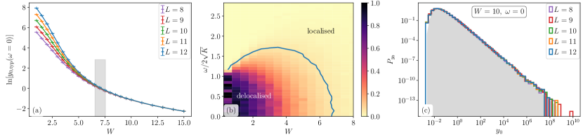
Figure 1: For a $K=2$ rooted Cayley tree, numerical results from the exact recursion method. (a) The typical $y_{0,\mathrm{typ}}$ at $\omega=0$, vs disorder strength $W$ (with $\Gamma\equiv 1$) for different total generation numbers $L$. For $W>W_{c}$, $y_{0,\mathrm{typ}}$ is independent of $L$; while for $W<W_{c}$ it grows with $L$, indicating a divergence in the thermodynamic limit. The critical $W_{c}$ subject to errorbars is the grey shaded region, estimated by positing $y_{0,\mathrm{typ}}=A+BN^{\beta}$; $\beta=0$ implies a localised phase and its deviation from 0 the onset of delocalisation. (b) Colour-map of $\beta$ as a function of $(W,\omega)$. The blue line shows the contour $\beta=0.05$ as an estimate of the critical line (mobility edges); the value is chosen in accordance with the errorbars in $\beta$. For $\omega=0$ our best estimate is $W_{c}(\omega=0)\simeq 6.8$. (c) Distribution of $y_{0}^{[L]}$ in the localised phase. Data are well converged for different $L$, and in excellent agreement with a Lévy distribution shown by the grey shaded region. Statistics are obtained over $5$$\times$$10^{4}$ disorder realisations.

Our analysis centres on the local Feenberg self-energy $S_{i}(\omega)\equiv X_{i}(\omega)-i\Delta_{i}(\omega)$, defined via the local propagator as $G_{i}(\omega)=[\omega^{+}-\epsilon_{i}-S_{i}(\omega)]^{-1}$ with $\omega^{+}=\omega+i\eta$ ($\eta=0^{+}$). We focus on the imaginary part of the self-energy, $\Delta_{i}(\omega)$, as it serves as a probabilistic order parameter for a localisation transition. Physically, $\Delta_{i}(\omega)$ gives the rate of loss of probability from site $i$ into states of energy $\omega$. In a delocalised phase $\Delta_{i}(\omega)$ is finite, whereas in a localised phase it vanishes $\propto\eta$ (with $y_{i}(\omega)=\Delta_{i}(\omega)/\eta$ finite), both with unit probability. These characteristics of $\Delta_{i}(\omega)$ have long been used successfully to understand Anderson transitions Anderson (1958); Economou and Cohen (1972); Abou-Chacra et al. (1973); Thouless (1974); Licciardello and Economou (1975); Logan and Wolynes (1985); *DELPGWPRB1987; and, more recently, MBL transitions on Fock space Logan and Welsh (2019); Roy and Logan (2019, 2020).

We focus on the self-energy of the root site ($i=0$) of the rooted Cayley tree. $S_{0}(\omega)$ is given exactly by

$$S_{0}^{\phantom{\dagger}}(\omega)=\Gamma^{2}\sum_{i_{1}\in\mathsf{N}[0]}[\omega^{+}-W\epsilon_{i_{1}}^{\phantom{\dagger}}-S_{i_{1}}^{(0)}]^{-1},$$ (3)

with the sum over all sites in the first generation, and $S_{i_{1}}^{(0)}$ the self-energy of site $i_{1}$ with the root site removed. One could in principle now approximate the self-energy on the right-hand side of Eq. (3) by a typical $S_{\mathrm{typ}}$, and obtain the distribution of $S_{0}$ self-consistently Logan and Welsh (2019); Roy and Logan (2019, 2020). Here however we go far beyond such a treatment, addressing Eq. (3) to arbitrarily high orders via an exact recursive method. We first sketch the formulation, focussing on the localised phase, in particular its stability and self-consistency; whence the quantity of interest is $y_{0}(\omega)$.

From Eq. (3), $y_{0}^{\phantom{\dagger}}(\omega)$ can be expressed as

$$y_{0}^{\phantom{\dagger}}=\sum_{i_{1}\in\mathsf{N}[0]}\frac{\Gamma^{2}}{\Omega_{i_{1}}^{2}}\left[1+y_{i_{1}}^{(0)}\right];~{}\Omega_{i_{1}}^{\phantom{\dagger}}=\omega-W\epsilon_{i_{1}}^{\phantom{\dagger}}-X_{i_{1}}^{(0)}.$$ (4)

This is a recursion relation, which can be iterated as

$$y_{0}^{\phantom{\dagger}}=\sum_{i_{1}\in\mathsf{N}[0]}\frac{\Gamma^{2}}{\Omega_{i_{1}}^{2}}\left[1+\sum_{i_{2}\in\mathsf{N}[i_{1}]}\frac{\Gamma^{2}}{\Omega_{i_{2}}^{2}}\left[1+\sum_{i_{3}\in\mathsf{N}[i_{2}]}\frac{\Gamma^{2}}{\Omega_{i_{3}}^{2}}[1+\cdots\right.\right..$$ (5)

In Eq. (5), for any site $i_{n}$ on generation $n$ of the tree, $\Omega_{i_{n}}=\omega-W\epsilon_{i_{n}}-X_{i_{n}}^{(i_{n-1})}(\omega)$, with $X_{i_{n}}^{(i_{n-1})}$ the real part of the self-energy of site $i_{n}$ with its (unique) neighbour $i_{n-1}$ on the previous generation removed. As for the imaginary part of the self-energy, a recursion relation for the real part can also be derived from Eq. (3). This leads to a recursion relation for $\Omega_{i_{n}}$,

$$\Omega_{i_{n}}^{\phantom{\dagger}}=\omega-W\epsilon_{i_{n}}^{\phantom{\dagger}}-\sum_{i_{n+1}\in\mathsf{N}[i_{n}]}\frac{\Gamma^{2}~{}~{}~{}}{\Omega_{i_{n+1}}^{2}},$$ (6)

with the boundary condition $\Omega_{i_{L}}=\omega-W\epsilon_{i_{L}}$ for a tree with $L$ generations. Eqs. (5),(6) comprise the complete set of recursion relations required to compute $y_{0}(\omega)$ to all orders. We now make key conceptual points about the stability of the localised phase or lack thereof, and describe our results.

Note that by evaluating $y_{0}(\omega)$ using Eq. (5) for many disorder realisations, one can generate its entire distribution $P_{y_{0}}$, and also compute its typical value via $\ln y_{0,\mathrm{typ}}^{{\phantom{\dagger}}}=\int dy_{0}~{}P_{y_{0}}(y_{0})\ln y_{0}$. A stable localised phase is indicated by $y_{0,\mathrm{typ}}^{{\phantom{\dagger}}}$ taking a finite value independent of system size; whereas the delocalised phase is identified via a systematic growth of $y_{0,\mathrm{typ}}^{{\phantom{\dagger}}}$ with system size, such that it diverges in the thermodynamic limit. The disorder strength separating these two behaviours, if present, is the critical disorder. Numerical results for the localisation phase digaram so obtained for a $K=2$ Cayley tree with maximally correlated disorder are shown in Fig. 1. Considering the band centre $\omega=0$ as an example (panel (a)), $\ln y_{0,\mathrm{typ}}^{{\phantom{\dagger}}}$ is independent of $L$ for $W>W_{c}$ whereas it diverges with $L$ for $W<W_{c}$; thus showing that a localisation transition is indeed present in the model. The phase diagram similarly obtained in the entire $\omega$-$W$ plane is given in Fig. 1(b), which shows the presence of mobility edges in the spectrum. Finally, Fig. 1(c), the distribution of $y_{0}$ is shown for a representative disorder in the localised phase, and shows excellent agreement with a Lévy distribution characteristic of a localised phase, $P_{y_{0}}(y_{0})=\sqrt{\kappa/\pi}~{}y_{0}^{-3/2}e^{-\kappa/y_{0}}$ with scale parameter $\kappa$.

The stability of the localised phase can also be understood as the convergence of the recursion relation in Eq. (5). The series for $y_{0}$ can be organised as

$$y_{0}^{\phantom{\dagger}}=\sum_{l=1}^{\infty}\phi_{l}^{\phantom{\dagger}};~{}\phi_{l}^{\phantom{\dagger}}=\sum_{i_{1}\in\mathsf{N}[0]}\frac{\Gamma^{2}}{\Omega_{i_{1}}^{2}}\sum_{i_{2}\in\mathsf{N}[i_{1}]}\frac{\Gamma^{2}}{\Omega_{i_{2}}^{2}}\cdots\sum_{i_{l}\in\mathsf{N}[i_{l-1}]}\frac{\Gamma^{2}}{\Omega_{i_{l}}^{2}},$$ (7)

with $\phi_{l}$ the total contribution to $y_{0}$ from all sites on the $l^{\mathrm{th}}$ generation. Diagrammatically, it is the total contribution to $y_{0}$ from all $K^{l}$ paths of length $2l$, each of which goes from the root site to a unique site in the $l^{\mathrm{th}}$ generation and retraces itself back to the root site . For the series in Eq. (4) to converge in the thermodynamic limit, $\phi_{l}$ must decrease sufficiently fast with increasing $l$. This suggests that the distributions $P_{\phi_{l}}$ of $\phi_{l}$, should evolve with $l$ in a qualitatively different manner in the delocalised and localised phases. Calculating $P_{\phi_{l}}$ shows that this is indeed so, as shown in Fig. 2(a)-(b). For strong disorder (localised phase), the vast bulk of the distribution shifts rapidly to smaller values with increasing $l$, while in the delocalised phase the support of the $P_{\phi_{l}}$ moves to larger values with increasing $l$. This is itself indicative of the convergence of the series in the localised phase and otherwise in the delocalised. To further quantify the convergence, one can define $y_{0}^{\scriptstyle{[l]}}\equiv\sum_{n=1}^{l}\phi_{n}$ and study its typical value, $y_{0,\mathrm{typ}}^{\scriptstyle{[l]}}$, as a function of $l$ and $W$. Representative results at $\omega=0$ are shown in Fig. 2(c). For weak disorder, $y_{0,\mathrm{typ}}^{\scriptstyle{[l]}}$ grows rapidly with $l$, whereas for strong disorder it saturates to its converged value in the localised phase; again clearly showing the presence of a localisation transition.

Two further remarks should be made. First, the recursive formulation also treats the real parts of all self-energies exactly. One can however make the simplifying approximation of neglecting them – Anderson’s ‘upper limit approximation’ Anderson (1958); Abou-Chacra et al. (1973). For the tree with correlated disorder this approximation again predicts the presence of a transition, albeit naturally at a higher $W_{c}$ sup . Second, the terms appearing in the series in Eq. (7) but with $X_{i_{n}}^{\scriptstyle{(i_{n-1})}}=0$ (i.e. $\Omega_{i_{n}}\equiv\omega-W\epsilon_{i_{n}}$) are precisely those appearing in the Forward Approximation Pietracaprina et al. (2016). By including the contribution of non-local propagators to the local propagator in an exact, fully renormalised fashion, the recursive formulation is a significant technical advance.

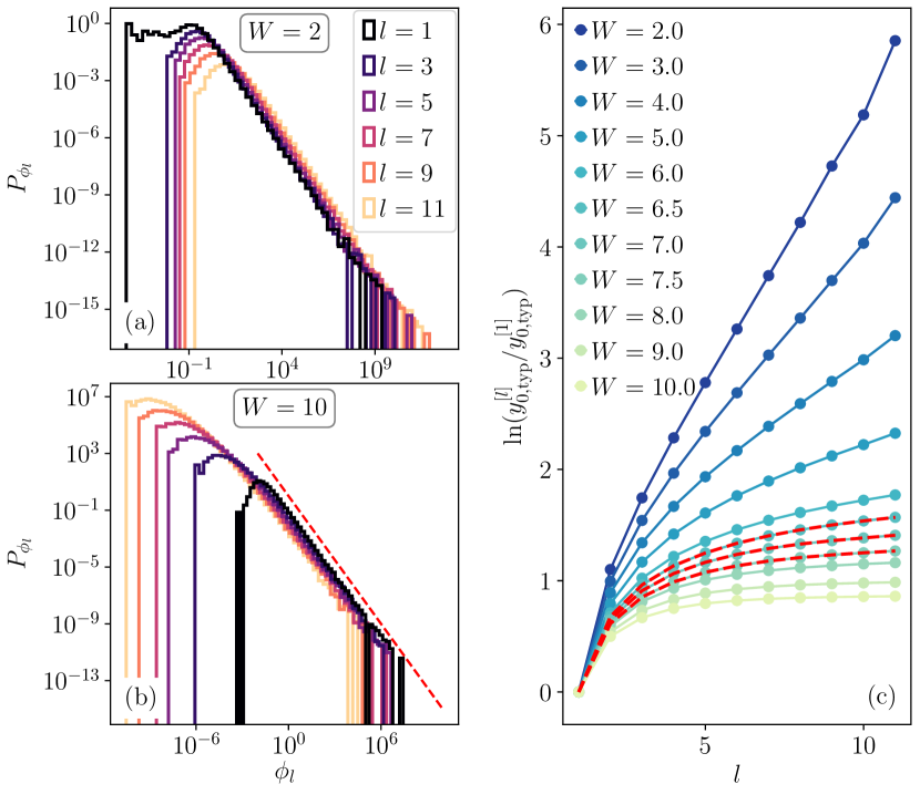
Figure 2: Convergence of the series for $y_{0}$ (Eq. (7)) for the $K=2$ Cayley tree. (a)-(b) Distributions $P_{\phi_{l}}$ in delocalised and localised phases, for different $l$; evolution with $l$ is qualitatively different in the two phases. Dashed line for localised phase shows Lévy tail, slope $-\tfrac{3}{2}$. (c) The typical value of the series summed to $l$ terms (normalised by the $l=1$ value) vs $l$. Results for $L=12$, $\omega=0$, and $5$$\times$$10^{4}$ realisations. Red lines show $W$ values lying in the critical regime shown in Fig. 1(a).

Correlations in the $\epsilon_{i}$’s preclude an exact analytic solution for the distribution of $y_{0}$ from Eq. (5). One can nevertheless perform a self-consistent mean-field calculation analytically at leading order in the renormalised perturbation series Logan and Welsh (2019); Roy and Logan (2020, 2019) (here illustrated for $\omega=0$). Here $y_{0}$ depends only on the site energies of its neighbours, $\{i_{1}\}$. Since $\ell_{0i_{1}}=1$, the maximally correlated limit implies the conditional distribution $P(\epsilon_{i_{1}}|\epsilon_{0})=\delta(\epsilon_{i_{1}}-\epsilon_{0})$ in the thermodynamic limit. The distribution of $y_{0}$ can thus be simply calculated as $P_{y_{0}}(y_{0})=\int d\epsilon_{0}~{}P(\epsilon_{0}^{\phantom{\dagger}})~{}\delta\big{(}y_{0}^{\phantom{\dagger}}-K\Gamma^{2}(1+y_{0,\mathrm{typ}}^{{\phantom{\dagger}}})/[W^{2}\epsilon_{0}^{2}]\big{)}$. Since the univariate distribution $P(\epsilon_{0})$ is a standard Normal, this yields $P_{y_{0}}(y_{0},y_{0,\mathrm{typ}}^{{\phantom{\dagger}}})=\sqrt{\kappa/\pi}~{}e^{-\kappa/y_{0}}y_{0}^{-3/2}$ where $\kappa=K(1+y_{0,\mathrm{typ}}^{{\phantom{\dagger}}})\Gamma^{2}/2W^{2}$. Remarkably and reassuringly, the distribution indeed has the Lévy form, just as obtained numerically by summing the entire series (Fig. 1(c)).

Self-consistency can now be imposed by requiring $\ln y_{0,\mathrm{typ}}^{{\phantom{\dagger}}}=\int dy_{0}P_{y_{0}}(y_{0},y_{0,\mathrm{typ}}^{{\phantom{\dagger}}})\ln y_{0}$; the solution of which is $y_{0,\mathrm{typ}}^{{\phantom{\dagger}}}=2e^{\gamma}K\Gamma^{2}(W^{2}-2e^{\gamma}K\Gamma^{2})^{-1}$, with $\gamma$ the Euler-Mascheroni constant. Since $y_{0}$ is necessarily non-negative, self-consistency of the localised phase requires $W\geq W_{c}$, with 

$$W_{c}^{\phantom{\dagger}}=\sqrt{2}e^{\gamma/2}\Gamma\sqrt{K}.$$ (8)

This $W_{c}\propto\sqrt{K}$ scaling is qualitatively different from that arising for uncorrelated disorder, where $W_{c}\propto K\ln K$ Abou-Chacra et al. (1973); and stems intrinsically from the maximal correlations in the disorder.

We turn now to results arising for RRGs, via exact diagonalisation (ED) of tight-binding Hamiltonians Eq. (1) with maximally correlated disorder Eq. (2). Our motivation here is twofold. First, while results above were for a rooted Cayley tree, we expect them to hold qualitatively for other random graphs. Second, it is important to corroborate the results with other independent measures of localisation. Cayley trees are not moreover readily amendable to ED, since a finite fraction of sites live on the boundary; this issue is sidestepped by considering RRGs, which are locally tree-like but contain long loops.

In the following we consider RRGs with a coordination number $Z=K+1=3$; denoting the total number of sites in the RRG by $N$. In accordance with the form of the covariance matrix for the Cayley tree, we take $C_{ij}=\exp[-\ell_{ij}\ln K/\ln N]$. The quantities studied will be the level spacing ratios, and $\Delta_{i}$ computed directly. We focus on the middle of the spectrum ($\omega=0$) and consider 50-100 eigenstates therein.

For an ordered set of eigenvalues $\{E_{n}\}$, the level spacing ratio is $r_{n}=\min[s_{n},s_{n+1}]/\max[s_{n},s_{n+1}]$ with $s_{n}=E_{n}-E_{n-1}$. In an ergodic phase the distribution of $r_{n}$ follows the Wigner-Dyson surmise with mean $\overline{r}\simeq 0.53$, while in a localised phase the distribution is Poisson with $\overline{r}\simeq 0.386$. Results for $\overline{r}$ vs $W$ are shown in Fig. 3(a), and show clearly a localisation transition. A scaling collapse of the data for various $N$ onto a common function of $(W-W_{c})N^{1/\nu}$ yields a critical disorder strength of $W_{c}\simeq 6.8$ and $\nu\simeq 4.6$. Note that the $W_{c}$ estimated is remarkably close to that obtained above numerically for the $K=2$ Cayley tree.

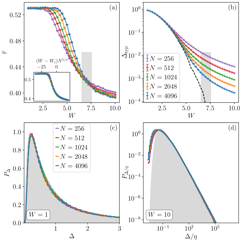
Figure 3: ED results for a $K=2$ RRG with maximally correlated disorder. (a) Mean level spacing ratio vs $W$ shows a crossing for different $N$. Data collapse onto a common function of $(W-W_{c})N^{1/\nu}$ yields $W_{c}\simeq 6.8$ and $\nu\simeq 4.6$ (inset). (b) Typical value $\Delta_{\mathrm{typ}}(\omega=0)$ computed exactly from Eq. (9). In the delocalised [localised] phase it is independent of [decays with] $N$. Dashed line shows extrapolation to $N\to\infty$. Grey shaded regions in (a), (b) denote the estimated critical region. (c)-(d) Distributions of $\Delta$ and $y=\Delta/\eta$ in the delocalised and localised phases respectively. Grey shaded regions show best fits to Log-Normal and Lévy distributions respectively.

From the set of exact eigenvalues $\{E_{n}\}$ and eigenstates $\{\ket{\psi_{n}}\}$, $\Delta_{i}(\omega)$ can be computed as

$$\Delta_{i}(\omega)=\mathrm{Im}[G_{i}^{-1}(\omega)]-\eta,~{}~{}G_{i}=\sum_{n}\frac{|\braket{\psi_{n}}{i}|^{2}}{\omega+i\eta-E_{n}}.$$ (9)

As $\Delta$ is finite with unit probability in the delocalised phase, $\Delta_{\mathrm{typ}}$ should converge to a finite value with increasing $N$; while in a localised phase $\Delta\propto\eta$ vanishes with unit probability, so $\Delta_{\mathrm{typ}}$ should decrease with $N$. This behaviour is indeed found, see Fig. 3(b). To estimate numerically the critical $W_{c}$, we posit $\Delta_{\mathrm{typ}}=\Delta_{\mathrm{typ},N\to\infty}+a/N^{\beta}$ and extrapolate the data to the thermodynamic limit. As shown in Fig. 3(b), the vanishing of $\Delta_{\mathrm{typ},N\to\infty}$ gives a $W_{c}$ consistent with that obtained from level statistics. In the localised phase, the distribution of $y=\Delta/\eta$ is again in very good agreement with a Lévy distribution (see Fig. 3(d)). In the delocalised phase by contrast, $\Delta$ is qualitatively different, and appears to be log-normally distributed (Fig. 3(c)).

As above, whether for a Cayley tree or RRG, we find a one-parameter Lévy distribution for $y=\Delta/\eta$ in the localised phase. Importantly, it is thus universal: distributions for different $W>W_{c}$ can be collapsed onto a universal form by scaling the self-energy as $y/y_{\mathrm{typ}}$ sup . Further, the distribution can be directly connected to that of wavefunction amplitudes, the moments of which (via generalised IPRs) probe the divergence of the localisation length, $\xi$, as $W\to W_{c}$ sup . Within our mean-field theory, we find $\xi\sim(W-W_{c})^{-1}$ with an exponent of $1$.

We turn now to the $K\to\infty$ limit. For any one-body problem to remain well-defined in this limit, the hopping must be rescaled as $\Gamma=\Gamma_{\ast}/\sqrt{K}$. The mean-field theory then yields a finite critical $W_{c}=\sqrt{2}e^{\gamma/2}\Gamma_{\ast}$; in stark contrast to the case of uncorrelated disorder where, despite rescaling $\Gamma$, $W_{c}/\Gamma_{\ast}\propto\sqrt{K}\ln K$ thus precludes localisation as $K\to\infty$. For MBL on Fock space, in a system containing $L$ real-space sites, the effective connectivity on the Fock-space graph scales as $K\sim L$, and the effective Fock-space disorder as $W_{\mathrm{FS}}\sim\sqrt{L}W_{\mathrm{t}}$ (with $W_{\mathrm{t}}\sim\mathcal{O}(1)$) Roy and Logan (2020); Logan and Welsh (2019). Rescaling all energies by $\sqrt{L}$, as required to attain a well-defined thermodynamic limit $L\to\infty$, again leads Roy and Logan (2020) to a finite critical $W_{\mathrm{t},c}$, in direct parallel to the $K\to\infty$ limit of the present problem. The existence of an MBL phase thus provides an indirect but complementary argument for the $\sqrt{K}$ scaling of $W_{c}$.

In summary, we have studied AL on Cayley trees and RRGs with maximally correlated on-site disorder, mimicking the effective Fock-space disorder of MBL systems. While such correlations might be thought to disfavour localisation by suppressing site-energy fluctuations, we find both that an Anderson transition is present, and that scaling of the critical disorder with graph connectivity is qualitatively different from that of uncorrelated disorder, with correlations favouring localisation. Our results address a new class of AL problems, and shed light on the crucial role played by correlations in Fock-space disorder in stabilising MBL. Many questions arise as to what further aspects of MBL can be captured by AL problems with maximally correlated disorder. One such is the multifractal character of wavefunctions, and its possible connection to the anomalous statistics of MBL wavefunctions on Fock space; and our preliminary results indeed suggest the presence of multifractal eigenstates on RRGs. Looking further afield, understanding the effect of maximal correlations on glassy dynamics on such graphs is also immanently important.

See pages 1 of supp.pdf See pages 2 of supp.pdf See pages 3 of supp.pdf