Cross-validation Confidence Intervals for Test Error

Abstract

This work develops central limit theorems for cross-validation and consistent estimators of its asymptotic variance under weak stability conditions on the learning algorithm. Together, these results provide practical, asymptotically-exact confidence intervals for $k$-fold test error and valid, powerful hypothesis tests of whether one learning algorithm has smaller $k$-fold test error than another. These results are also the first of their kind for the popular choice of leave-one-out cross-validation. In our real-data experiments with diverse learning algorithms, the resulting intervals and tests outperform the most popular alternative methods from the literature.

1 Introduction

Cross-validation (CV) [49, 26] is a de facto standard for estimating the test error of a prediction rule. By partitioning a dataset into $k$ equal-sized validation sets, fitting a prediction rule with each validation set held out, evaluating each prediction rule on its corresponding held-out set, and averaging the $k$ error estimates, CV produces an unbiased estimate of the test error with lower variance than a single train-validation split could provide. However, these properties alone are insufficient for high-stakes applications in which the uncertainty of an error estimate impacts decision-making. In predictive cancer prognosis and mortality prediction for instance, scientists and clinicians rely on test error confidence intervals (CIs) based on CV and other repeated sample splitting estimators to avoid spurious findings and improve reproducibility [42, 45]. Unfortunately, the CIs most often used have no correctness guarantees and can be severely misleading [30]. The difficulty comes from the dependence across the $k$ averaged error estimates: if the estimates were independent, one could derive an asymptotically-exact CI (i.e., a CI with coverage converging exactly to the target level) for test error using a standard central limit theorem. However, the error estimates are seldom independent, due to the overlap amongst training sets and between different training and validation sets. Thus, new tools are needed to develop valid, informative CIs based on CV.

The same uncertainty considerations are relevant when comparing two machine learning methods: before selecting a prediction rule for deployment, one would like to be confident that its test error is better than a baseline or an available alternative. The standard practice amongst both method developers and consumers is to conduct a formal hypothesis test for a difference in test error between two prediction rules [22, 38, 43, 13, 19]. Unfortunately, the most popular tests from the literature like the cross-validated $t$-test [22], the repeated train-validation $t$-test [43], and the $5\times 2$ CV test [22] have no correctness guarantees and hence can produce misleading conclusions. The difficulty parallels that of the confidence interval setting: standard tests assume independence and do not appropriately account for the dependencies across CV error estimates. Therefore, new tools are also needed to develop valid, powerful tests for test error improvement based on CV.

Our contributions

To meet these needs, we characterize the asymptotic distribution of CV error and develop consistent estimates of its variance under weak stability conditions on the learning algorithm. Together, these results provide practical, asymptotically-exact confidence intervals for test error as well as valid and powerful hypothesis tests of whether one learning algorithm has smaller test error than another. In more detail, we prove in Sec. 2 that $k$-fold CV error is asymptotically normal around its test error under an abstract asymptotic linearity condition. We then give in Sec. 3 two different stability conditions that hold for large classes of learning algorithms and losses and that individually imply the asymptotic linearity condition. In Sec. 4, we propose two estimators of the asymptotic variance of CV and prove them to be consistent under similar stability conditions; our second estimator accommodates any choice of $k$ and appears to be the first consistent variance estimator for leave-one-out CV. To validate our theory in Sec. 5, we apply our intervals and tests to a diverse collection of classification and regression methods on particle physics and flight delay data and observe consistent improvements in width and power over the most popular alternative methods from the literature.

Related work

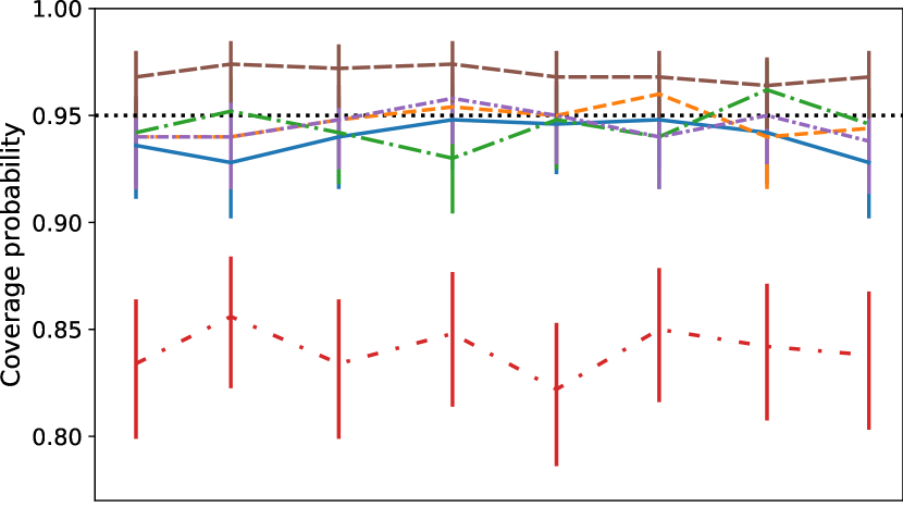
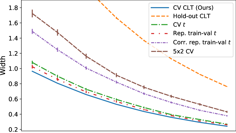
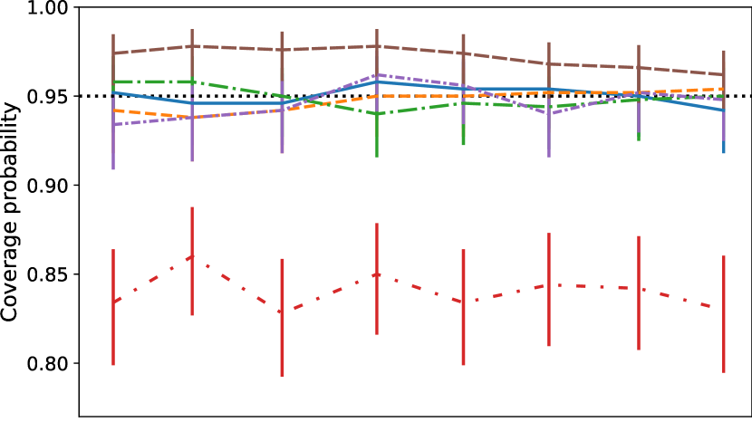
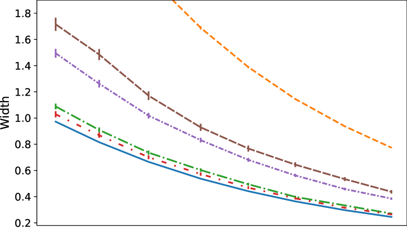
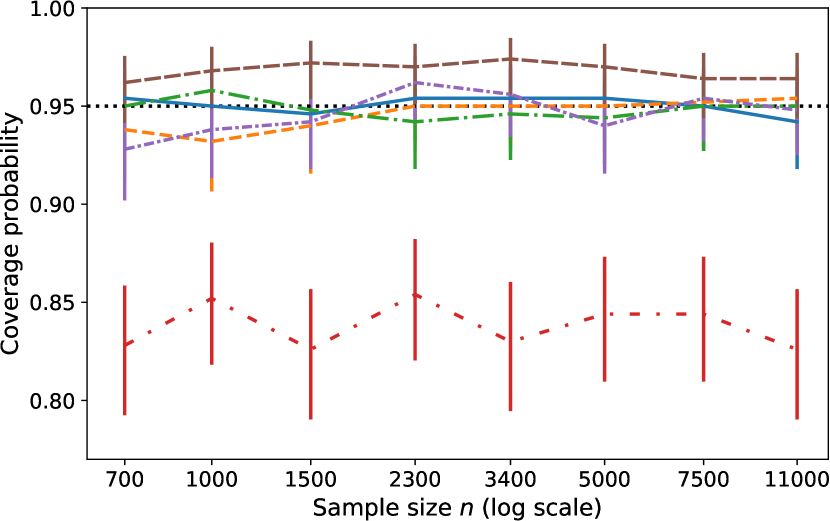
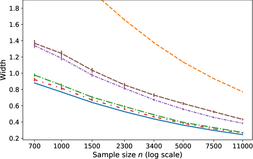
Figure 5: Test error coverage (left) and width (right) of $95\%$ confidence intervals (see Sec. 5.1). Top: Random forest regression. Middle: Ridge regression. Bottom: Neural network regression.

Despite the ubiquity of CV, we are only aware of three prior efforts to characterize the precise distribution of cross-validation error. The CV central limit theorem (CLT) of Dudoit and van der Laan, [23] requires considerably stronger assumptions than our own and is not paired with the consistent estimate of variance needed to construct a valid confidence interval or test. LeDell et al., [36] derive both a CLT and a consistent estimate of variance for CV, but these apply only to the area under the ROC curve (AUC) performance measure. Finally, in very recent work, Austern and Zhou, [5] derive a CLT and a consistent estimate of variance for CV under more stringent assumptions than our own. We compare our results with each of these works in detail in Sec. 3.3. We note also that another work [37] aims to test the difference in test error between two learning algorithms using cross-validation but only proves the validity of their procedure for a single train-validation split rather than for CV. Many other works have studied the problem of bounding or estimating the variance of the cross-validation error [11, 43, 9, 39, 31, 34, 16, 2, 3], but none have established the consistency of their variance estimators. Among these, Kale et al., [31], Kumar et al., [34], Celisse and Guedj, [16] introduce relevant notions of algorithmic stability to which we link our results in Sec. 3.1. Moreover, non-asymptotic CIs can be derived from the CV concentration inequalities of [14, 18, 16, 2, 3], but these CIs are more difficult to deploy as they require (1) stronger stability assumptions, (2) a known upper bound on stability, and (3) either a known upper bound on the loss or a known uniform bound on the covariates and a known sub-Gaussianity constant for the response variable. In addition, the reliance on somewhat loose inequalities typically leads to overly large, relatively uninformative CIs. For example, we implemented the ridge regression CI of [16, Thm. 3] for the regression experiment of Sec. 5.1 (see Sec. K.3). When the features are standardized, the narrowest concentration-based interval is 91 times wider than our widest CLT interval in Fig. 5. Without standardization, the narrowest concentration-based interval is $5\times 10^{14}$ times wider.

Notation

Let $\stackrel{{\scriptstyle d}}{{\to}}$, $\stackrel{{\scriptstyle p}}{{\to}}$, and $\stackrel{{\scriptstyle L^{q}}}{{\to}}$ for $q>0$, denote convergence in distribution, in probability, and in $L^{q}$ norm (i.e., $X_{n}\stackrel{{\scriptstyle L^{q}}}{{\to}}X\Leftrightarrow\mathbb{E}[|X_{n}-X|^{q}]\to 0$), respectively. For each $m,n\in\mathbb{N}$ with $m\leq n$, we define the set $[n]\triangleq\{1,\dots,n\}$ and the vector $m\colon n\triangleq(m,\dots,n)$. When considering independent random elements $(X,Y)$, we use $\mathbb{E}_{X}$ and $\mathrm{Var}_{X}$ to indicate expectation and variance only over $X$, respectively; that is, $\mathbb{E}_{X}\mathopen{}\mathclose{{}\left[{f(X,Y)}}\right]\triangleq\mathbb{E}[f(X,Y)\mid Y]$ and $\mathrm{Var}_{X}(f(X,Y))\triangleq\mathrm{Var}(f(X,Y)\mid Y)$. We will refer to the Euclidean norm of a vector as the $\ell^{2}$ norm in the context of $\ell^{2}$ regularization.

2 A Central Limit Theorem for Cross-validation

In this section, we present a new central limit theorem for $k$-fold cross-validation. Throughout, any asymptotic statement will take $n\to\infty$, and while we allow the number of folds $k_{n}$ to depend on the sample size $n$ (e.g., $k_{n}=n$ for leave-one-out cross-validation), we will write $k$ in place of $k_{n}$ to simplify our notation. We will also present our main results assuming that $k$ evenly divides $n$, but we address the indivisible setting in the appendix.

Hereafter, we will refer to a sequence $(Z_{i})_{i\geq 1}$ of random datapoints taking values in a set $\mathcal{Z}$. Notably, $(Z_{i})_{i\geq 1}$ need not be independent or identically distributed. We let $Z_{1:n}$ designate the first $n$ points, and, for any vector $B$ of indices in $[n]$, we let $Z_{B}$ denote the subvector of $Z_{1:n}$ corresponding to ordered indices in $B$. We will also refer to train-validation splits $(B,B^{\prime})$. These are vectors of indices in $[n]$ representing the ordered points assigned to the training set and validation set. As is typical in CV, we will assume that $B$ and $B^{\prime}$ partition $[n]$, so that every datapoint is either in the training or validation set.

Given a scalar loss function $h_{n}(Z_{i},Z_{B})$ and a set of $k$ train-validation splits $\{(B_{j},B_{j}^{\prime})\}_{j=1}^{k}$ with validation indices $\{B_{j}^{\prime}\}_{j=1}^{k}$ partitioning $[n]$ into $k$ folds, we will use the $k$-fold cross-validation error

$$\textstyle\hat{R}_{n}\triangleq\frac{1}{n}\sum_{j=1}^{k}\sum_{i\in B_{j}^{\prime}}h_{n}(Z_{i},Z_{B_{j}})$$ (2.1)

to draw inferences about the $k$-fold test error

$$\textstyle R_{n}\triangleq\frac{1}{n}\sum_{j=1}^{k}\sum_{i\in B_{j}^{\prime}}\mathbb{E}[h_{n}(Z_{i},Z_{B_{j}})\mid Z_{B_{j}}].$$ (2.2)

A prototypical example of $h_{n}$ is squared error or 0-1 loss,

$$h_{n}(Z_{i},Z_{B})=(Y_{i}-\hat{f}(X_{i};Z_{B}))^{2}\quad\text{or}\quad h_{n}(Z_{i},Z_{B})=\mathbbm{1}[{Y_{i}\neq\hat{f}(X_{i};Z_{B})}],$$

composed with an algorithm for fitting a prediction rule $\hat{f}(\cdot;Z_{B})$ to training data $Z_{B}$ and predicting the response value of a test point $Z_{i}=(X_{i},Y_{i})$. In this setting, the $k$-fold test error is a standard inferential target [11, 23, 31, 34, 5] and represents the average test error of the $k$ prediction rules $\hat{f}(\cdot;Z_{B_{j}})$. When comparing the performance of two algorithms in Secs. 4 and 5, we will choose $h_{n}$ to be the difference between the losses of two prediction rules.

2.1 Asymptotic linearity of cross-validation

The key to our central limit theorem is establishing that the $k$-fold CV error asymptotically behaves like the $k$-fold test error plus an average of functions applied to single datapoints. The following proposition provides a convenient characterization of this asymptotic linearity property.

Proposition 1 (Asymptotic linearity of $k$-fold CV).

For any sequence of datapoints $(Z_{i})_{i\geq 1}$,

$$\textstyle\frac{\sqrt{n}}{\sigma_{n}}(\hat{R}_{n}-R_{n})-\frac{1}{\sigma_{n}\sqrt{n}}\sum_{i=1}^{n}\mathopen{}\mathclose{{}\left(\bar{h}_{n}(Z_{i})-\mathbb{E}\mathopen{}\mathclose{{}\left[\bar{h}_{n}(Z_{i})}\right]}\right)\stackrel{{\scriptstyle p}}{{\to}}\Big{(}\text{resp.\,}\stackrel{{\scriptstyle L^{q}}}{{\to}}\Big{)}\;0$$ (2.3)

for a function $\bar{h}_{n}$ with $\sigma_{n}^{2}\triangleq\frac{1}{n}\mathrm{Var}(\sum_{i=1}^{n}\bar{h}_{n}(Z_{i}))$ if and only if

$$\textstyle{\textstyle\frac{1}{\sigma_{n}\sqrt{n}}}\sum_{j=1}^{k}\sum_{i\in B_{j}^{\prime}} \textstyle\Big{(}h_{n}\mathopen{}\mathclose{{}\left(Z_{i},Z_{B_{j}}}\right)-\mathbb{E}\mathopen{}\mathclose{{}\left[h_{n}\mathopen{}\mathclose{{}\left(Z_{i},Z_{B_{j}}}\right)\mid Z_{B_{j}}}\right]$$ (2.4)

$$\textstyle-\mathopen{}\mathclose{{}\left(\bar{h}_{n}(Z_{i})-\mathbb{E}\mathopen{}\mathclose{{}\left[\bar{h}_{n}(Z_{i})}\right]}\right)\Big{)}\stackrel{{\scriptstyle p}}{{\to}}\Big{(}\text{resp.\,}\stackrel{{\scriptstyle L^{q}}}{{\to}}\Big{)}\;0,\;$$ (2.5)

where the parenthetical convergence indicates that the same statement holds when both convergences in probability are replaced with convergences in $L^{q}$ for the same $q>0$.

Typically, one will choose $\bar{h}_{n}(z)=\mathbb{E}[h_{n}(z,Z_{1:n(1-1/k)})]$. With this choice, we see that the difference of differences in 2.4 is small whenever $h_{n}(Z_{i},Z_{B_{j}})$ is close to either its expectation given $Z_{i}$ or its expectation given $Z_{B_{j}}$, but it need not be close to both. As the asymptotic linearity condition 2.4 is still quite abstract, we devote all of Sec. 3 to establishing sufficient conditions for 2.4 that are interpretable, broadly applicable, and simple to verify. Prop. 1 follows from a more general asymptotic linearity characterization for repeated sample-splitting estimators proved in App. A.

2.2 From asymptotic linearity to asymptotic normality

So far, we have assumed nothing about the dependencies amongst the datapoints $Z_{i}$. If we additionally assume that the datapoints are i.i.d., the average $\frac{1}{\sigma_{n}\sqrt{n}}\sum_{i=1}^{n}\mathopen{}\mathclose{{}\left(\bar{h}_{n}(Z_{i})-\mathbb{E}\mathopen{}\mathclose{{}\left[\bar{h}_{n}(Z_{i})}\right]}\right)$ converges to a standard normal under a mild integrability condition, and we obtain the following CLT for CV.

Theorem 1 (Asymptotic normality of $k$-fold CV with i.i.d. data).

In the notation of Prop. 1, suppose that the datapoints $(Z_{i})_{i\geq 1}$ are i.i.d. copies of a random element $Z_{0}$ and that the sequence of $(\bar{h}_{n}(Z_{0})-\mathbb{E}[\bar{h}_{n}(Z_{0})])^{2}/\sigma_{n}^{2}$ with $\sigma_{n}^{2}=\operatorname{Var}(\bar{h}_{n}(Z_{0}))$ is uniformly integrable (UI). If the asymptotic linearity condition 2.4 holds in probability then

$$\textstyle\frac{\sqrt{n}}{\sigma_{n}}(\hat{R}_{n}-R_{n})\stackrel{{\scriptstyle d}}{{\to}}\mathcal{N}(0,1).$$ (2.6)

Thm. 1 is a special case of a more general result, proved in App. B, that applies when the datapoints are independent but not necessarily identically distributed. A simple sufficient condition for the required uniform integrability is that $\sup_{n}\mathbb{E}[|(\bar{h}_{n}(Z_{0})-\mathbb{E}[\bar{h}_{n}(Z_{0})])/\sigma_{n}|^{\alpha}]<\infty$ for some $\alpha>2$. This holds, for example, whenever $\bar{h}_{n}(Z_{0})$ has uniformly bounded $\alpha$ moments (e.g., the 0-1 loss has all moments uniformly bounded) and does not converge to a degenerate distribution. We now turn our attention to the asymptotic linearity condition.

3 Sufficient Conditions for Asymptotic Linearity

3.1 Asymptotic linearity from loss stability

Our first result relates the asymptotic linearity of CV to a specific notion of algorithmic stability, termed loss stability.

Definition 1 (Mean-square stability and loss stability).

For $m>0$, let $Z_{0}$ and $Z_{0}^{\prime},Z_{1},\ldots,Z_{m}$ be i.i.d. test and training points with $Z^{\backslash i}_{1:m}$ representing $Z_{1:m}$ with $Z_{i}$ replaced by $Z_{0}^{\prime}$. For any function $h:\mathcal{Z}\times\mathcal{Z}^{m}\to\mathbb{R}$, the mean-square stability [31] is defined as

$$\textstyle\gamma_{ms}(h)\triangleq\frac{1}{m}\sum_{i=1}^{m}\mathbb{E}[(h(Z_{0},Z_{1:m})-h(Z_{0},Z^{\backslash i}_{1:m}))^{2}]$$ (3.1)

and the loss stability [34] as $\gamma_{loss}(h)\triangleq\gamma_{ms}(h^{\prime})$, where

$$\textstyle h^{\prime}(Z_{0},Z_{1:m})\triangleq h(Z_{0},Z_{1:m})-\mathbb{E}\mathopen{}\mathclose{{}\left[h(Z_{0},Z_{1:m})\mid Z_{1:m}}\right].$$ (3.2)

Kumar et al., [34] introduced loss stability to bound the variance of CV in terms of the variance of a single hold-out set estimate. Here we show that a suitable decay in loss stability is also sufficient for $L^{2}$ asymptotic linearity, via a non-asymptotic bound on the departure from linearity.

Theorem 2 (Approximate linearity from loss stability).

In the notation of Prop. 1 and Def. 1, suppose that the datapoints $(Z_{i})_{i\geq 1}$ are i.i.d. copies of a random element $Z_{0}$. Then

$$\textstyle\mathrm{Var}(\frac{1}{\sqrt{n}}\sum_{j=1}^{k}\sum_{i\in B_{j}^{\prime}}(h^{\prime}_{n}(Z_{i},Z_{B_{j}})-\mathbb{E}[h^{\prime}_{n}(Z_{i},Z_{B_{j}})\mid Z_{i}]))\leq\frac{3}{2}n\mathopen{}\mathclose{{}\left(1-\frac{1}{k}}\right)\gamma_{loss}(h_{n}).$$ (3.3)

Hence the $L^{2}$ asymptotic linearity condition 2.4 holds with $\bar{h}_{n}(z)=\mathbb{E}[h_{n}(z,Z_{1:n(1-1/k)})]$ if the loss stability satisfies $\gamma_{loss}(h_{n})=o(\sigma_{n}^{2}/n)$.

The proof of Thm. 2 is given in App. C. Recall that in a typical learning context, we have $h_{n}(Z_{0},Z_{1:m})=\ell(Y_{0},\hat{f}(X_{0};Z_{1:m}))$ for a fixed loss $\ell$, a learned prediction rule $\hat{f}(\cdot;Z_{1:m})$, a test point $Z_{0}=(X_{0},Y_{0})$, and $m=n\mathopen{}\mathclose{{}\left(1-1/k}\right)$. When $\hat{f}(\cdot;Z_{1:m})$ converges to an imperfect prediction rule, we will commonly have $\sigma_{n}^{2}=\mathrm{Var}(\mathbb{E}\mathopen{}\mathclose{{}\left[h_{n}(Z_{0},Z_{1:m})\mid Z_{0}}\right])=\Omega(1)$ so that $\gamma_{loss}(h_{n})=o(1/n)$ loss stability is sufficient. However, Thm. 2 also accommodates the cases of non-convergent $\hat{f}(\cdot;Z_{1:m})$ and of $\hat{f}(\cdot;Z_{1:m})$ converging to a perfect prediction rule, so that $\sigma_{n}^{2}=o(1)$.

Many learning algorithms are known to enjoy decaying loss stability [14, 25, 29, 16, 4], in part because loss stability is upper-bounded by a variety of algorithmic stability notions studied in the literature. For example, stochastic gradient descent on convex and non-convex objectives [29] and the empirical risk minimization of a strongly convex and Lipschitz objective both have $O(1/n)$ uniform stability [14] which implies a loss stability of $O(1/n^{2})=o(1/n)$ by [31, Lem. 1] and [34, Lem. 2]. However, we emphasize that the loss $h_{n}$ need not be convex and need not coincide with a loss function used to train a learning method. Indeed, our stability assumptions also cover $k$-nearest neighbor methods [20], decision tree methods [4], and ensemble methods [25] and can even hold when training error is a poor proxy for test error due to overfitting (e.g., 1-nearest neighbor has training error 0 but is still suitably stable [20]). In addition, for any loss function, loss stability is upper-bounded by mean-square stability [31] and all $L^{q}$ stabilities [16] for $q\geq 2$. For bounded loss functions such as the 0-1 loss, loss stability is also weaker than hypothesis stability (also called $L^{1}$ stability) [20, 32], weak-hypothesis stability [21], and weak-$L^{1}$ stability [35].

3.2 Asymptotic linearity from conditional variance convergence

We can also guarantee asymptotic linearity under weaker moment conditions than Thm. 2 at the expense of stronger requirements on the number of folds $k$.

Theorem 3 (Asymptotic linearity from conditional variance convergence).

In the notation of Prop. 1, suppose that the datapoints $(Z_{i})_{i\geq 1}$ are i.i.d. copies of a random element $Z_{0}$. If

$$\textstyle\max(k^{q/2},k^{1-q/2})\mathbb{E}\Big{[}\big{(}\frac{1}{\sigma_{n}^{2}}\mathrm{Var}_{Z_{0}}\mathopen{}\mathclose{{}\left(h_{n}(Z_{0},Z_{1:n(1-1/k)})-\bar{h}_{n}(Z_{0})}\right)\big{)}^{q/2}\Big{]}\to 0$$ (3.4)

for a function $\bar{h}_{n}$ and $q\in(0,2]$, then $\bar{h}_{n}$ satisfies the $L^{q}$ asymptotic linearity condition 2.4. If

$$\textstyle\mathbb{E}\mathopen{}\mathclose{{}\left[{\min\Big{(}k,\frac{\sqrt{k}}{\sigma_{n}}\sqrt{\mathrm{Var}_{Z_{0}}\mathopen{}\mathclose{{}\left(h_{n}(Z_{0},Z_{1:n(1-1/k)})-\bar{h}_{n}(Z_{0})}\right)}\Big{)}}}\right]\to 0.$$ (3.5)

for a function $\bar{h}_{n}$, then $\bar{h}_{n}$ satisfies the in-probability asymptotic linearity condition 2.4.

Remark 1.

When $k=O(1)$, 3.5 holds $\Leftrightarrow$ $\frac{1}{\sigma_{n}}\sqrt{\mathrm{Var}_{Z_{0}}\mathopen{}\mathclose{{}\left(h_{n}(Z_{0},Z_{1:n(1-1/k)})-\bar{h}_{n}(Z_{0})}\right)}\stackrel{{\scriptstyle p}}{{\to}}0$.

Thm. 3 follows from a more general statement proved in App. D. When $k$ is bounded, as in $10$-fold CV, the conditions of Thm. 3 are considerably weaker than those of Thm. 2 (see App. E), granting asymptotic linearity whenever the conditional variance converges in probability rather than in $L^{2}$. Indeed in App. G, we detail a simple learning problem in which the loss stability is infinite but Thms. 3 and 1 together provide a valid CLT with convergent variance $\sigma_{n}^{2}$.

3.3 Comparison with prior work

Our sufficient conditions for asymptotic normality are significantly less restrictive and more broadly applicable than the three prior distributional characterizations of CV error [23, 36, 5]. In particular, the CLT of Dudoit and van der Laan, [23, Thm. 3] assumes a bounded loss function, excludes the popular case of leave-one-out cross-validation, and requires the prediction rule to be loss-consistent for a risk-minimizing prediction rule. Similarly, the CLT of LeDell et al., [36, Thm. 4.1] applies only to AUC loss, requires the prediction rule to be loss-consistent for a deterministic prediction rule, and requires a bounded number of folds.

Moreover, in our notation, the recent CLT of Austern and Zhou, [5, Thm. 1] restricts focus to learning algorithms that treat all training points symmetrically, assumes that its variance parameter

$$\tilde{\sigma}_{n}^{2}\triangleq\mathbb{E}[\mathrm{Var}(h_{n}(Z_{0},Z_{1:m})\mid Z_{1:m})]$$ (3.6)

converges to a non-zero limit, requires mean-square stability $\gamma_{ms}(h_{n})=o(1/n)$, and places a $o(1/n^{2})$ constraint on the second-order mean-square stability

$$\textstyle\mathbb{E}[((h_{n}(Z_{0},Z_{1:m})-h_{n}(Z_{0},Z^{\backslash 1}_{1:m}))-(h_{n}(Z_{0},Z^{\backslash 2}_{1:m})-h_{n}(Z_{0},Z^{\backslash 1,2}_{1:m})))^{2}]=o(1/n^{2}),$$ (3.7)

where $Z^{\backslash 1,2}_{1:m}$ represents $Z_{1:m}$ with $Z_{1}$, $Z_{2}$ replaced by i.i.d. copies $Z^{\prime}_{1}$, $Z^{\prime}_{2}$. Kumar et al., [34] showed that the mean-square stability is always an upper bound for the loss stability required by our Thm. 2, and in Apps. F and G we exhibit two simple learning tasks in which $\gamma_{loss}(h_{n})=O(1/n^{2})$ but $\gamma_{ms}(h_{n})=\infty$. Furthermore, when $k$ is constant, as in $10$-fold CV, our conditional variance assumptions in Sec. 3.2 are weaker still and hold even for algorithms with infinite loss stability (see App. G). In addition, our results allow for asymmetric learning algorithms (like stochastic gradient descent), accommodate growing, vanishing, and non-convergent variance parameters $\sigma_{n}^{2}$, and do not require the second-order mean-square stability condition 3.7.

Finally, we note that the asymptotic variance parameter $\sigma_{n}^{2}$ appearing in Thm. 1 is never larger and sometimes smaller than the variance parameter $\tilde{\sigma}_{n}^{2}$ in [5, Thm. 1].

Proposition 2 (Variance comparison).

Let $\sigma_{n}^{2}=\mathrm{Var}(\mathbb{E}[h_{n}(Z_{0},Z_{1:m})\mid Z_{0}])$ be the variance appearing in Thm. 1, with the choice $\bar{h}_{n}(z)=\mathbb{E}[h_{n}(z,Z_{1:m})]$, and $\tilde{\sigma}_{n}^{2}=\mathbb{E}[\mathrm{Var}(h_{n}(Z_{0},Z_{1:m})\mid Z_{1:m})]$ be the variance parameter of [5, Eq. (15)] for $m=n\mathopen{}\mathclose{{}\left(1-1/k}\right)$. Then

$$\textstyle\sigma_{n}^{2}\leq\tilde{\sigma}_{n}^{2}\leq\sigma_{n}^{2}+\frac{m}{2}\gamma_{loss}(h_{n}),$$ (3.8)

and the first inequality is strict whenever $h(Z_{0},Z_{1:m})-\mathbb{E}\mathopen{}\mathclose{{}\left[h(Z_{0},Z_{1:m})\mid Z_{1:m}}\right]$ depends on $Z_{1:m}$.

The proof of Prop. 2 can be found in App. H. In App. G, we present a simple learning task for which our central limit theorem provably holds with $\sigma_{n}^{2}$ converging to a non-zero constant, but the CLT in [5, Eq. (15)] is inapplicable because the variance parameter $\tilde{\sigma}_{n}^{2}$ is infinite.

4 Confidence Intervals and Tests for $k$-fold Test Error

A primary application of our central limit theorems is the construction of asymptotically-exact confidence intervals for the unknown $k$-fold test error. For example, under the assumptions and notation of Thm. 1, any sample statistic $\hat{\sigma}_{n}^{2}$ satisfying relative error consistency, $\hat{\sigma}_{n}^{2}/\sigma_{n}^{2}\stackrel{{\scriptstyle p}}{{\to}}1$, gives rise to an asymptotically-exact $(1-\alpha)$-confidence interval,

$$\textstyle C_{\alpha}\triangleq\hat{R}_{n}\pm q_{1-\alpha/2}\hat{\sigma}_{n}/\sqrt{n}\quad\text{satisfying}\quad\lim_{n\to\infty}\mathbb{P}(R_{n}\in C_{\alpha})=1-\alpha,$$ (4.1)

where $q_{1-\alpha/2}$ is the $(1-\alpha/2)$-quantile of a standard normal distribution.

A second, related application of our central limit theorems is testing whether, given a dataset $Z_{1:n}$, a $k$-fold partition $\{B_{j}^{\prime}\}_{j=1}^{k}$, and two algorithms $\mathcal{A}_{1}$, $\mathcal{A}_{2}$ for fitting prediction rules, $\mathcal{A}_{2}$ has larger $k$-fold test error than $\mathcal{A}_{1}$. In this circumstance, we may define

$$\textstyle h_{n}(Z_{0},Z_{B})=\ell(Y_{0},\hat{f}_{1}(X_{0};Z_{B}))-\ell(Y_{0},\hat{f}_{2}(X_{0};Z_{B}))$$ (4.2)

to be the difference of the loss functions of two prediction rules trained on $Z_{B}$ and tested on $Z_{0}=(X_{0},Y_{0})$. Our aim is to test whether $\mathcal{A}_{1}$ improves upon $\mathcal{A}_{2}$ on the fold partition, that is to test the null $H_{0}:R_{n}\geq 0$ against the alternative hypothesis $H_{1}:R_{n}<0$. Under the assumptions and notation of Thm. 1, an asymptotically-exact level-$\alpha$ test is given by

$$\textstyle\textsc{reject }H_{0}\Leftrightarrow\hat{R}_{n}<q_{\alpha}\hat{\sigma}_{n}/\sqrt{n}$$ (4.3)

where $q_{\alpha}$ is the $\alpha$-quantile of a standard normal distribution and $\hat{\sigma}_{n}^{2}$ is any variance estimator satisfying relative error consistency, $\hat{\sigma}_{n}^{2}/\sigma_{n}^{2}\stackrel{{\scriptstyle p}}{{\to}}1$. Fortunately, our next theorem describes how to compute such a consistent estimate of $\sigma_{n}^{2}$ under weak conditions.

Theorem 4 (Consistent within-fold estimate of asymptotic variance).

In the notation of Thm. 1 with $m=n(1-1/k)$, $\bar{h}_{n}(z)=\mathbb{E}[h_{n}(z,Z_{1:m})]$, and $k<n$, define the within-fold variance estimator

$$\textstyle\hat{\sigma}_{n,in}^{2}\triangleq\frac{1}{k}\sum_{j=1}^{k}\frac{1}{(n/k)-1}\sum_{i\in B_{j}^{\prime}}\mathopen{}\mathclose{{}\left(h_{n}(Z_{i},Z_{B_{j}})-\frac{k}{n}\sum_{i^{\prime}\in B_{j}^{\prime}}h_{n}(Z_{i^{\prime}},Z_{B_{j}})}\right)^{2}.$$ (4.4)

Suppose $(Z_{i})_{i\geq 1}$ are i.i.d. copies of a random element $Z_{0}$. Then $\hat{\sigma}_{n,in}^{2}/\sigma_{n}^{2}\stackrel{{\scriptstyle L^{1}}}{{\to}}1$ whenever $\gamma_{loss}(h_{n})=o(\sigma_{n}^{2}/n)$ and the sequence of $(\bar{h}_{n}(Z_{0})-\mathbb{E}[\bar{h}_{n}(Z_{0})])^{2}/\sigma_{n}^{2}$ is uniformly integrable (UI). Moreover, $\hat{\sigma}_{n,in}^{2}/\sigma_{n}^{2}\stackrel{{\scriptstyle L^{2}}}{{\to}}1$ whenever $\mathbb{E}[((\bar{h}_{n}(Z_{0})-\mathbb{E}[\bar{h}_{n}(Z_{0})])/\sigma_{n})^{4}]=o(n)$ and the fourth-moment loss stability $\gamma_{4}(h_{n}^{\prime})\triangleq\frac{1}{m}\sum_{i=1}^{m}\mathbb{E}[(h_{n}^{\prime}(Z_{0},Z_{1:m})-h_{n}^{\prime}(Z_{0},Z_{1:m}^{\backslash i}))^{4}]=o(\sigma_{n}^{4}/n^{2})$. Here, $Z^{\backslash i}_{1:m}$ denotes $Z_{1:m}$ with $Z_{i}$ replaced by an identically distributed copy independent of $Z_{0:m}$.

Thm. 4 follows from explicit error bounds proved in App. I. A notable take-away is that the same two conditions—loss stability $\gamma_{loss}(h_{n})=o(\sigma_{n}^{2}/n)$ and a UI sequence of $(\bar{h}_{n}(Z_{0})-\mathbb{E}[\bar{h}_{n}(Z_{0})])^{2}/\sigma_{n}^{2}$—grant both a central limit theorem for CV (by Thms. 1 and 2) and an $L^{1}$-consistent estimate of $\sigma_{n}^{2}$ (by Thm. 4). Moreover, the $L^{2}$-consistency bound of App. I can be viewed as a strengthening of the consistency result of [5, Prop. 1] which analyzes the same variance estimator under more stringent assumptions. In our notation, to establish $L^{2}$ consistency, [5, Prop. 1] additionally requires $h_{n}$ symmetric in its training points, convergence of the variance parameter $\tilde{\sigma}_{n}^{2}$ 3.6 to a non-zero constant, control over a fourth-moment analogue of mean-square stability $\gamma_{4}(h_{n})=o(\sigma_{n}^{4}/n^{2})$ instead of the smaller fourth-moment loss stability $\gamma_{4}(h_{n}^{\prime})$, and the more restrictive fourth-moment condition $\mathbb{E}[(h_{n}(Z_{0},Z_{1:m})/\sigma_{n})^{4}]=O(1)$. By Prop. 2, their assumptions further imply that $\sigma_{n}^{2}$ converges to a non-zero constant. In contrast, Thm. 4 accommodates growing, vanishing, and non-convergent variance parameters $\sigma_{n}^{2}$ and a wider variety of learning procedures and losses.

Since Thm. 4 necessarily excludes the case of leave-one-out CV ($k=n$), we propose a second estimator with consistency guarantees for any $k$ and only slightly stronger stability conditions than Thm. 4 when $k=\Omega(n)$. Notably, Austern and Zhou, [5] do not provide a consistent variance estimator for $k=n$, and Dudoit and van der Laan, [23] do not establish the consistency of any variance estimator.

Theorem 5 (Consistent all-pairs estimate of asymptotic variance).

Under the notation of Thm. 1 with $m=n(1-1/k)$, and $\bar{h}_{n}(z)=\mathbb{E}[h_{n}(z,Z_{1:m})]$, define the all-pairs variance estimator

$$\textstyle\hat{\sigma}_{n,out}^{2}\triangleq\frac{1}{k}\sum_{j=1}^{k}\frac{k}{n}\sum_{i\in B_{j}^{\prime}}(h_{n}(Z_{i},Z_{B_{j}})-\hat{R}_{n})^{2}.$$ (4.5)

If $(Z_{i})_{i\geq 1}$ are i.i.d. copies of a random element $Z_{0}$, then $\hat{\sigma}_{n,out}^{2}/\sigma_{n}^{2}\stackrel{{\scriptstyle L^{1}}}{{\to}}1$ whenever $\gamma_{loss}(h_{n})=o(\sigma_{n}^{2}/n)$, $\gamma_{ms}(h_{n})=o(k\sigma_{n}^{2}/n)$, and the sequence of $(\bar{h}_{n}(Z_{0})-\mathbb{E}[\bar{h}_{n}(Z_{0})])^{2}/\sigma_{n}^{2}$ is UI.

Thm. 5 follows from an explicit error bound proved in App. J and differs from the $L^{1}$-consistency result of Thm. 4 only in the added requirement $\gamma_{ms}(h_{n})=o(k\sigma_{n}^{2}/n)$. This mean-square stability condition is especially mild when $k=\Omega(n)$ (as in the case of leave-one-out CV) and ensures that two training sets differing in only $n/k$ points produce prediction rules with comparable test losses.

Importantly, both $\hat{\sigma}_{n,in}^{2}$ and $\hat{\sigma}_{n,out}^{2}$ can be computed in $O(n)$ time using just the individual datapoint losses $h_{n}(Z_{i},Z_{B_{j}})$ outputted by a run of $k$-fold cross-validation. Moreover, when $h_{n}$ is binary, as in the case of 0-1 loss, one can compute $\hat{\sigma}_{n,out}^{2}=\hat{R}_{n}(1-\hat{R}_{n})$ in $O(1)$ time given access to the overall cross-validation error $\hat{R}_{n}$ and $\hat{\sigma}_{n,in}^{2}=\frac{1}{k}\sum_{j=1}^{k}\frac{(n/k)}{(n/k)-1}\hat{R}_{n,j}(1-\hat{R}_{n,j})$ in $O(k)$ time given access to the $k$ average fold errors $\hat{R}_{n,j}\triangleq\frac{k}{n}\sum_{i\in B_{j}^{\prime}}h_{n}(Z_{i},Z_{B_{j}})$.

5 Numerical Experiments

In this section, we compare our test error confidence intervals 4.1 and tests for algorithm improvement 4.3 with the most popular alternatives from the literature: the hold-out test described in [5, Eq. (17)] based on a single train-validation split, the cross-validated $t$-test [22], the repeated train-validation $t$-test [43] (with and without correction), and the $5\times 2$-fold CV test [22]. These procedures are commonly used and admit both two-sided CIs and one-sided tests, but, unlike our proposals, none except the hold-out method are known to be valid. Our aim is to verify whether our proposed procedures outperform these popular heuristics across a diversity of settings encountered in real learning problems. We fix $k=10$, use $90$-$10$ train-validation splits for all tests save $5\times 2$-fold CV, and report our results using $\hat{\sigma}_{n,out}^{2}$ (as $\hat{\sigma}_{n,in}^{2}$ results are nearly identical).

Evaluating the quality of CIs and tests requires knowledge of the target test error. In each experiment, we use points subsampled from a large real dataset to form a surrogate ground-truth estimate of the test error. Then, we evaluate the CIs and tests constructed from $500$ training sets of sample sizes $n$ ranging from $700$ to $11,000$ subsampled from the same dataset. Each mean width estimate is displayed with a $\pm$ 2 standard error confidence band. The surrounding confidence bands for the coverage, size, and power estimates are $95\%$ Wilson intervals [51], which are known to provide more accurate coverage for binomial proportions than a $\pm$ 2 standard error interval [15]. We use the Higgs dataset of [6, 7] to study the classification error of random forest, neural network, and $\ell^{2}$-penalized logistic regression classifiers and the Kaggle FlightDelays dataset of [1] to study the mean-squared regression error of random forest, neural network, and ridge regression. In each case, we focus on stable settings of these learning algorithms with sufficiently strong $\ell^{2}$ regularization for the neural network, logistic, and ridge learners and small depths for the random forest trees. Complete experimental details are available in Sec. K.1, and code replicating all experiments can be found at https://github.com/alexandre-bayle/cvci.

5.1 Confidence intervals for test error

In Sec. L.1, we compare the coverage and width of each procedure’s $95\%$ CI for each of the described algorithms, datasets, and training set sizes. Two representative examples—logistic regression classification and random forest regression—are displayed in Fig. 1. While the repeated train-validation CI significantly undercovers in all cases, all remaining CIs have coverage near the $95\%$ target, even for the smallest training set size of $n=700$. The hold-out CI, while valid, is substantially wider and less informative than the other intervals as it is based on only a single train-validation split. Meanwhile, our CLT-based CI delivers the smallest width (and hence greatest precision) for both learning tasks and every dataset size.

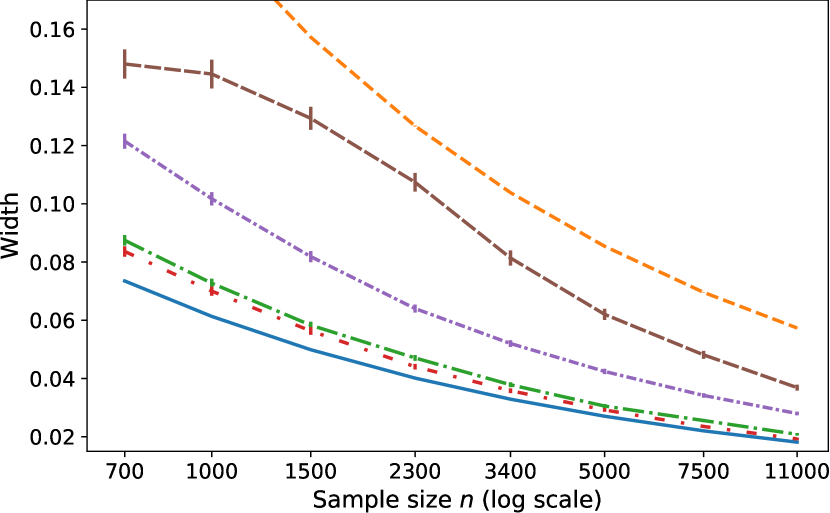
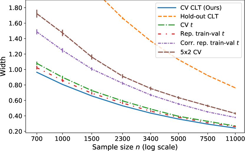
Figure 1: Test error coverage (top) and width (bottom) of $95\%$ confidence intervals (see Sec. 5.1). Left: $\ell^{2}$-regularized logistic regression classifier. Right: Random forest regression.

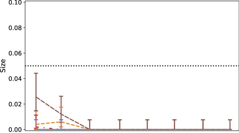
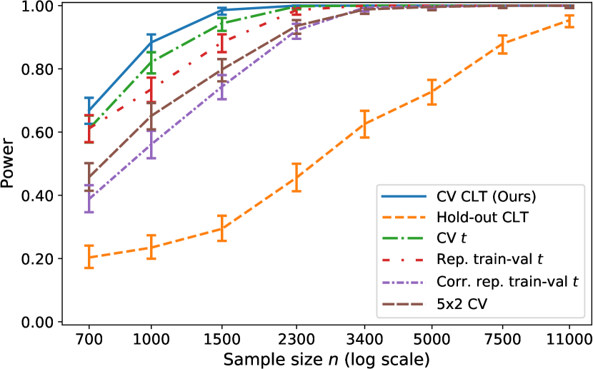
Figure 2: Size when testing $H_{1}:\text{Err}(\mathcal{A}_{1})<\text{Err}(\mathcal{A}_{2})$ (top) and power when testing $H_{1}:\text{Err}(\mathcal{A}_{2})<\text{Err}(\mathcal{A}_{1})$ (bottom) of level-$0.05$ tests for improved test error (see Sec. 5.2). Left: $\mathcal{A}_{1}=$ $\ell^{2}$-regularized logistic regression, $\mathcal{A}_{2}=$ neural network classification. Right: $\mathcal{A}_{1}=$ random forest, $\mathcal{A}_{2}=$ ridge regression.

5.2 Testing for improved algorithm performance

Let us write $\text{Err}(\mathcal{A}_{1})<\text{Err}(\mathcal{A}_{2})$ to signify that the test error of $\mathcal{A}_{1}$ is smaller than that of $\mathcal{A}_{2}$. In Sec. L.2, for each testing procedure, dataset, and pair of algorithms $(\mathcal{A}_{1},\mathcal{A}_{2})$, we display the size and power of level $\alpha=0.05$ one-sided tests 4.3 of $H_{1}:\text{Err}(\mathcal{A}_{1})<\text{Err}(\mathcal{A}_{2})$. In each case, we report size estimates for experiments with at least 25 replications under the null and power estimates for experiments with at least 25 replications under the alternative. Here, for representative algorithm pairs, we identify the algorithm $\mathcal{A}_{1}$ that more often has smaller test error across our simulations and display both the power of the level $\alpha=0.05$ test of $H_{1}:\text{Err}(\mathcal{A}_{1})<\text{Err}(\mathcal{A}_{2})$ and the size of the level $\alpha=0.05$ test of $H_{1}:\text{Err}(\mathcal{A}_{2})<\text{Err}(\mathcal{A}_{1})$. Fig. 2 displays these results for $(\mathcal{A}_{1},\mathcal{A}_{2})$ = ($\ell^{2}$-regularized logistic regression, neural network) classification on the left and $(\mathcal{A}_{1},\mathcal{A}_{2})$ = (random forest, ridge) regression on the right. The sizes of all testing procedures are below the nominal level of $0.05$, and our test is consistently the most powerful for both classification and regression. The hold-out test, while also valid, is significantly less powerful due to its reliance on a single train-validation split. In Sec. L.3, we observe analogous results when labels are synthetically generated.

5.3 The importance of stability

To illustrate the impact of algorithmic instability on testing procedures, we additionally compare a less stable neural network (with substantially reduced $\ell^{2}$ regularization strength) and a less stable random forest regressor (with larger-depth trees). In Fig. 13 in Sec. L.4, we observe that the size of every test save the hold-out test rises above the nominal level. In the case of our test, the cause of this size violation is clear. Fig. 15(a) in Sec. L.4 demonstrates that the variance of $\frac{\sqrt{n}}{\sigma_{n}}(\hat{R}_{n}-R_{n})$ in Thm. 1 is much larger than $1$ for this experiment, and Thm. 2 implies this can only occur when the loss stability $\gamma_{loss}(h_{n})$ is large. Meanwhile, the variance of the same quantity is close to $1$ for the original stable settings of the neural network and random forest regressors. We suspect that instability is also the cause of the other tests’ size violations; however, it is difficult to be certain, as these alternative tests have no correctness guarantees. Interestingly, the same destabilized algorithms produce high-quality confidence intervals and relatively stable $h_{n}$ in the context of single algorithm assessment (see Figs. 14 and 15(b) in Sec. L.4), as the variance parameter $\sigma_{n}^{2}=\mathrm{Var}(\bar{h}_{n}(Z_{0}))$ is significantly larger for single algorithms. This finding highlights an important feature of our results: it suffices for the loss stability to be negligible relative to the noise level $\sigma_{n}^{2}/n$.

5.4 Leave-one-out cross-validation

Leave-one-out cross-validation (LOOCV) is often viewed as prohibitive for large datasets, due to the expense of refitting a prediction rule $n$ times. However, for ridge regression, a well-known shortcut based on the Sherman–Morrison–Woodbury formula allows one to carry out LOOCV exactly in the time required to fit a small number of base ridge regressions (see Sec. K.4 for a derivation of this result). Moreover, recent work shows that, for many learning procedures, LOOCV estimates can be efficiently approximated with only $O(1/n^{2})$ error [8, 28, 33, 50] (see also [46, 48, 27] for related guarantees). The $O(1/n^{2})$ precision of these inexpensive approximations coupled with the LOOCV consistency of $\hat{\sigma}_{n,out}^{2}$ (see Thm. 5) allows us to efficiently construct asymptotically-valid CIs and tests for LOOCV, even when $n$ is large. As a simple demonstration, we construct $95\%$ CIs for ridge regression test error based on our LOOCV CLT and compare their coverage and width with those of the procedures described in Sec. 5.1. In Fig. 3 in Sec. K.4, we see that, like the 10-fold CV CLT intervals, the LOOCV intervals provide coverage near the nominal level and widths smaller than the popular alternatives from the literature; in fact, the 10-fold CV CLT curves are obscured by the nearly identical LOOCV CLT curves. Complete experimental details can be found in Sec. K.4.

6 Conclusion and Future Work

Our central limit theorems and consistent variance estimators provide new, valid tools for testing algorithm improvement and generating test error intervals under algorithmic stability. An important open question is whether practical valid tests and intervals are also available when our stability conditions are violated. Another promising direction for future work is developing analogous tools for the expected test error $\mathbb{E}[R_{n}]$ instead of the $k$-fold test error $R_{n}$; Austern and Zhou, [5] provide significant progress in this direction, but more work, particularly on variance estimation, is needed.

Broader Impact

This work will benefit both users and developers of machine learning methods who want to rigorously assess or compare learning algorithms. Failure of the methods we discuss (which can only happen when the assumptions we state are not satisfied) may lead to the over- or under-estimation of the performance of a learning algorithm on a particular dataset.

Appendix A Proof of Prop. 1: Asymptotic linearity of $k$-fold CV

We first prove a general asymptotic linearity result for repeated sample-splitting estimators. Given a collection $A_{n}=\{(B_{j},B^{\prime}_{j})\}_{j\in[J]}$ of index vector pairs such that for any pair $(B_{j},B^{\prime}_{j})$ in $A_{n}$, $B_{j}$ and $B^{\prime}_{j}$ are disjoint, and a scalar loss function $\rho_{n,j}(Z_{B_{j}^{\prime}},Z_{B_{j}})$, define the cross-validation error as

$$\textstyle\hat{R}_{n}=\frac{1}{J}\sum_{j=1}^{J}\rho_{n,j}(Z_{B_{j}^{\prime}},Z_{B_{j}})$$ (A.1)

and the multi-fold test error

$$\textstyle R_{n}=\frac{1}{J}\sum_{j=1}^{J}\mathbb{E}[\rho_{n,j}(Z_{B_{j}^{\prime}},Z_{B_{j}})\mid Z_{B_{j}}].$$ (A.2)

Note that similarly to the number of folds $k$ in cross-validation, $J$ can depend on the sample size $n$, but we write $J$ in place of $J_{n}$ to simplify our notation.

Proposition 3 (Asymptotic linearity of CV).

For any sequence of datapoints $(Z_{i})_{i\geq 1}$,

$$\textstyle\frac{\sqrt{n}}{\sigma_{n}}\mathopen{}\mathclose{{}\left(\hat{R}_{n}-R_{n}}\right)-\frac{\sqrt{n}}{\sigma_{n}J}\sum_{j=1}^{J}(\bar{\rho}_{n,j}(Z_{B_{j}^{\prime}})-\mathbb{E}[\bar{\rho}_{n,j}(Z_{B_{j}^{\prime}})])\stackrel{{\scriptstyle p}}{{\to}}\Big{(}\text{resp.\,}\stackrel{{\scriptstyle L^{q}}}{{\to}}\Big{)}\;0$$ (A.3)

for functions $\bar{\rho}_{n,1},\dots,\bar{\rho}_{n,J}$ with $\sigma_{n}^{2}\triangleq\frac{1}{J}\mathrm{Var}(\sum_{j=1}^{J}\bar{\rho}_{n,j}(Z_{B_{j}^{\prime}}))$ if and only if

$$\textstyle\frac{\sqrt{n}}{\sigma_{n}J}\sum_{j=1}^{J} \textstyle\Big{(}\rho_{n,j}(Z_{B_{j}^{\prime}},Z_{B_{j}})-\mathbb{E}\mathopen{}\mathclose{{}\left[\rho_{n,j}(Z_{B_{j}^{\prime}},Z_{B_{j}})\mid Z_{B_{j}}}\right]$$ (A.4)

$$\textstyle-\mathopen{}\mathclose{{}\left(\bar{\rho}_{n,j}(Z_{B_{j}^{\prime}})-\mathbb{E}\mathopen{}\mathclose{{}\left[\bar{\rho}_{n,j}(Z_{B_{j}^{\prime}})}\right]}\right)\Big{)}\stackrel{{\scriptstyle p}}{{\to}}\Big{(}\text{resp.\,}\stackrel{{\scriptstyle L^{q}}}{{\to}}\Big{)}\;0$$ (A.5)

where the parenthetical convergence indicates that the same statement holds when both convergences in probability are replaced with convergences in $L^{q}$ for the same $q>0$.

Proof    For each $(B_{j},B^{\prime}_{j})\in A_{n}$, let

$$\textstyle L_{j}=\rho_{n,j}(Z_{B_{j}^{\prime}},Z_{B_{j}})-\mathbb{E}[\rho_{n,j}(Z_{B_{j}^{\prime}},Z_{B_{j}})\mid Z_{B_{j}}]-\mathopen{}\mathclose{{}\left(\bar{\rho}_{n,j}(Z_{B_{j}^{\prime}})-\mathbb{E}[\bar{\rho}_{n,j}(Z_{B_{j}^{\prime}})]}\right).$$ (A.6)

Then

$$\textstyle\frac{\sqrt{n}}{\sigma_{n}}\mathopen{}\mathclose{{}\left(\hat{R}_{n}-R_{n}}\right) \textstyle=\frac{\sqrt{n}}{\sigma_{n}J}\sum_{j=1}^{J}(\rho_{n,j}(Z_{B_{j}^{\prime}},Z_{B_{j}})-\mathbb{E}[\rho_{n,j}(Z_{B_{j}^{\prime}},Z_{B_{j}})\mid Z_{B_{j}}])$$ (A.7)

$$\textstyle=\frac{\sqrt{n}}{\sigma_{n}J}\sum_{j=1}^{J}L_{j}+\frac{\sqrt{n}}{\sigma_{n}J}\sum_{j=1}^{J}(\bar{\rho}_{n,j}(Z_{B_{j}^{\prime}})-\mathbb{E}[\bar{\rho}_{n,j}(Z_{B_{j}^{\prime}})]).$$ (A.8)

The result now follows from the assumption that $\frac{\sqrt{n}}{\sigma_{n}J}\sum_{j=1}^{J}L_{j}\stackrel{{\scriptstyle p}}{{\to}}\Big{(}\text{resp.\,}\stackrel{{\scriptstyle L^{q}}}{{\to}}\Big{)}\;0$. ∎

Prop. 1 now follows directly from Prop. 3 with the choices:

• $A_{n}=\{(B_{\ell},i):\ell\in[k],i\in B_{\ell}^{\prime}\}$,

• for all $j\in[J]$, $\rho_{n,j}(Z_{i},Z_{B_{\ell}})=h_{n}(Z_{i},Z_{B_{\ell}})$ and $\bar{\rho}_{n,j}(Z_{i})=\bar{h}_{n}(Z_{i})$ for the associated $\ell\in[k]$ and $i\in B_{\ell}^{\prime}$.

Note that for these choices, we have $J=|A_{n}|=\sum_{\ell=1}^{k}|B_{\ell}^{\prime}|=n$.

Appendix B Proof of Thm. 1: Asymptotic normality of $k$-fold CV with i.i.d. data

Thm. 1 follows from the next more general result, which establishes the asymptotic normality of $k$-fold CV with independent (not necessarily identically distributed) data.

Theorem 6 (Asymptotic normality of $k$-fold CV with independent data).

Under the notation of Prop. 1, suppose that the datapoints $(Z_{i})_{i\geq 1}$ are independent. If the triangular array $\mathopen{}\mathclose{{}\left(\bar{h}_{n}(Z_{i})-\mathbb{E}\mathopen{}\mathclose{{}\left[\bar{h}_{n}(Z_{i})}\right]}\right)_{n,i}$ satisfies Lindeberg’s condition,

$$\textstyle\forall\varepsilon>0,\frac{1}{n\sigma_{n}^{2}}\sum_{i=1}^{n}\mathbb{E}\mathopen{}\mathclose{{}\left[\mathopen{}\mathclose{{}\left(\bar{h}_{n}(Z_{i})-\mathbb{E}\mathopen{}\mathclose{{}\left[\bar{h}_{n}(Z_{i})}\right]}\right)^{2}\mathbbm{1}\mathopen{}\mathclose{{}\left[{|\bar{h}_{n}(Z_{i})-\mathbb{E}\mathopen{}\mathclose{{}\left[\bar{h}_{n}(Z_{i})}\right]|>\varepsilon\,\sigma_{n}\sqrt{n}}}\right]}\right]\to 0,$$ (B.1)

then

$$\textstyle\frac{1}{\sigma_{n}\sqrt{n}}\sum_{i=1}^{n}\mathopen{}\mathclose{{}\left(\bar{h}_{n}(Z_{i})-\mathbb{E}\mathopen{}\mathclose{{}\left[\bar{h}_{n}(Z_{i})}\right]}\right)\stackrel{{\scriptstyle d}}{{\to}}\mathcal{N}(0,1).$$ (B.2)

Additionally, if 2.4 holds in probability, then

$$\textstyle\frac{\sqrt{n}}{\sigma_{n}}\mathopen{}\mathclose{{}\left(\hat{R}_{n}-R_{n}}\right)\stackrel{{\scriptstyle d}}{{\to}}\mathcal{N}(0,1).$$ (B.3)

Proof    By independence of the datapoints $(Z_{i})_{i\geq 1}$, $(\bar{h}_{n}(Z_{i}))_{n,i}$ are independent, and $n\sigma_{n}^{2}=\mathrm{Var}(\sum_{i=1}^{n}\bar{h}_{n}(Z_{i}))$. Under Lindeberg’s condition, we get the first convergence result thanks to Lindeberg’s Central Limit Theorem (see [10, Thm. 27.2]). Additionally, if assumption 2.4 holds, we apply Prop. 1 and Slutsky’s theorem to get the second convergence result. ∎

If the $(Z_{i})_{i\geq 1}$ are i.i.d., then $\sigma_{n}^{2}=\frac{1}{n}\mathrm{Var}(\sum_{i=1}^{n}\bar{h}_{n}(Z_{i}))=\mathrm{Var}(\bar{h}_{n}(Z_{0}))$, and Lindeberg’s condition B.1 reduces to

$$\textstyle\forall\varepsilon>0,\frac{1}{\sigma_{n}^{2}}\mathbb{E}\mathopen{}\mathclose{{}\left[\mathopen{}\mathclose{{}\left(\bar{h}_{n}(Z_{0})-\mathbb{E}\mathopen{}\mathclose{{}\left[\bar{h}_{n}(Z_{0})}\right]}\right)^{2}\mathbbm{1}\mathopen{}\mathclose{{}\left[{|\bar{h}_{n}(Z_{0})-\mathbb{E}\mathopen{}\mathclose{{}\left[\bar{h}_{n}(Z_{0})}\right]|>\varepsilon\,\sigma_{n}\sqrt{n}}}\right]}\right]\to 0.$$ (B.4)

We will show that this follows from the assumed uniform integrability of the sequence $X_{n}=(\bar{h}_{n}(Z_{0})-\mathbb{E}[\bar{h}_{n}(Z_{0})])^{2}/\sigma_{n}^{2}$. Indeed, for any $\varepsilon>0$ and all $n$,

$$\textstyle\mathbb{E}[X_{n}\mathbbm{1}\mathopen{}\mathclose{{}\left[{X_{n}>n\varepsilon^{2}}}\right]] \textstyle\leq\sup_{m}\mathbb{E}[X_{m}\mathbbm{1}\mathopen{}\mathclose{{}\left[{X_{m}>n\varepsilon^{2}}}\right]]\to 0,$$ (B.5)

as $n\to\infty$ by the uniform integrability of the sequence of $X_{n}$. Thm. 1 therefore follows from Thm. 6.

Appendix C Proof of Thm. 2: Approximate linearity from loss stability

Thm. 2 will follow from the following more general result.

Theorem 7 (Approximate linearity from loss stability).

Under the notation of App. A, with $\{(B_{j},B^{\prime}_{j})\}_{j\in[J]}$ a collection of disjoint index vector pairs where $(B_{j}^{\prime})_{j\in[J]}$ is a pairwise disjoint family, and $\rho_{n,j}(Z_{B_{j}^{\prime}},Z_{B_{j}})\triangleq\frac{1}{|B_{j}^{\prime}|}\sum_{i\in B_{j}^{\prime}}h_{n,j}(Z_{i},Z_{B_{j}})$, suppose that the datapoints $(Z_{i})_{i\geq 1}$ are i.i.d. copies of a random element $Z_{0}$. Define $\rho_{n,j}^{\prime}(Z_{B_{j}^{\prime}},Z_{B_{j}})\triangleq\rho_{n,j}(Z_{i},Z_{B_{j}})-\mathbb{E}[\rho_{n,j}(Z_{i},Z_{B_{j}})\mid Z_{B_{j}}]$ and $\rho_{n,j}^{\prime\prime}(Z_{B_{j}^{\prime}},Z_{B_{j}})\triangleq\rho_{n,j}^{\prime}(Z_{i},Z_{B_{j}})-\mathbb{E}[\rho_{n,j}^{\prime}(Z_{i},Z_{B_{j}})\mid Z_{i}]$. Then

$$\textstyle\mathbb{E}[(\frac{1}{J}\sum_{j=1}^{J}\rho_{n,j}^{\prime\prime}(Z_{B_{j}^{\prime}},Z_{B_{j}}))^{2}]\leq\frac{1}{J^{2}} \textstyle\Big{(}\sum_{j\neq j^{\prime}}\sqrt{\gamma_{loss}(h_{n,j})\gamma_{loss}(h_{n,j^{\prime}})}$$ (C.1)

$$\textstyle+\sum_{j=1}^{J}\frac{1}{|B_{j}^{\prime}|}\frac{1}{2}|B_{j}|\gamma_{loss}(h_{n,j})\Big{)}.$$ (C.2)

Proof

Define $h_{n,j}^{\prime}$ and $h_{n,j}^{\prime\prime}$ as:

$h_{n,j}^{\prime}(Z_{i},Z_{B_{j}})\triangleq h_{n,j}(Z_{i},Z_{B_{j}})-\mathbb{E}[h_{n,j}(Z_{i},Z_{B_{j}})\mid Z_{B_{j}}]$,

$h_{n,j}^{\prime\prime}(Z_{i},Z_{B_{j}})\triangleq h_{n,j}^{\prime}(Z_{i},Z_{B_{j}})-\mathbb{E}[h_{n,j}^{\prime}(Z_{i},Z_{B_{j}})\mid Z_{i}]$.

Therefore, we have $\rho_{n,j}^{\prime}(Z_{B_{j}^{\prime}},Z_{B_{j}})=\frac{1}{|B_{j}^{\prime}|}\sum_{i\in B_{j}^{\prime}}h_{n,j}^{\prime}(Z_{i},Z_{B_{j}})$ and $\rho_{n,j}^{\prime\prime}(Z_{B_{j}^{\prime}},Z_{B_{j}})=\frac{1}{|B_{j}^{\prime}|}\sum_{i\in B_{j}^{\prime}}h_{n,j}^{\prime\prime}(Z_{i},Z_{B_{j}})$.

Thus

$$\textstyle(\frac{1}{J}\sum_{j=1}^{J}\rho_{n,j}^{\prime\prime}(Z_{B_{j}^{\prime}},Z_{B_{j}}))^{2} \textstyle=\frac{1}{J^{2}}\sum_{j,j^{\prime}=1}^{J}\rho_{n,j}^{\prime\prime}(Z_{B_{j}^{\prime}},Z_{B_{j}})\rho_{n,j^{\prime}}^{\prime\prime}(Z_{B_{j^{\prime}}^{\prime}},Z_{B_{j^{\prime}}})$$ (C.3)

$$\textstyle=\frac{1}{J^{2}}\sum_{j,j^{\prime}=1}^{J}\frac{1}{|B_{j}^{\prime}|}\frac{1}{|B_{j^{\prime}}^{\prime}|}\sum_{i\in B_{j}^{\prime}}\sum_{{i^{\prime}}\in B_{j^{\prime}}^{\prime}}h_{n,j}^{\prime\prime}(Z_{i},Z_{B_{j}})h_{n,j^{\prime}}^{\prime\prime}(Z_{i^{\prime}},Z_{B_{j^{\prime}}}).$$ (C.4)

In what follows, $Z_{B_{j^{\prime}}}^{\backslash{i}}$ is $Z_{B_{j^{\prime}}}$ with $Z_{i}$ replaced by $Z_{0}^{\prime}$, an i.i.d. copy of $Z_{0}$, independent of $(Z_{i})_{i\geq 1}$. Note that if $i\notin B_{j^{\prime}}$, $Z_{B_{j^{\prime}}}^{\backslash{i}}$ is just $Z_{B_{j^{\prime}}}$. We similarly define $Z_{B_{j}}^{\backslash{i^{\prime}}}$.

If $j\neq j^{\prime}$, we have $\mathbb{E}_{Z_{i}}[\sum_{i\in B_{j}^{\prime}}\sum_{i^{\prime}\in B_{j^{\prime}}^{\prime}}h_{n,j}^{\prime\prime}(Z_{i},Z_{B_{j}})h_{n,j^{\prime}}^{\prime\prime}(Z_{i^{\prime}},Z_{B_{j^{\prime}}}^{\backslash{i}})]=0$, because (i) $h_{n,j}^{\prime\prime}(Z_{i},Z_{B_{j}})$ and $h_{n,j^{\prime}}^{\prime\prime}(Z_{i^{\prime}},Z_{B_{j^{\prime}}}^{\backslash{i}})$ are conditionally independent given everything but $Z_{i}$, and (ii) $\mathbb{E}_{Z_{i}}[h_{n,j}^{\prime\prime}(Z_{i},Z_{B_{j}})]=0$.

Similarly, if $j\neq j^{\prime}$,

$$\textstyle\mathbb{E}_{Z_{i^{\prime}}}[\sum_{i\in B_{j}^{\prime}}\sum_{i^{\prime}\in B_{j^{\prime}}^{\prime}}h_{n,j}^{\prime\prime}(Z_{i},Z_{B_{j}}^{\backslash{i^{\prime}}})h_{n,j^{\prime}}^{\prime\prime}(Z_{i^{\prime}},Z_{B_{j^{\prime}}})]=0,$$ (C.5)

$$\textstyle\mathbb{E}_{Z_{i^{\prime}}}[\sum_{i\in B_{j}^{\prime}}\sum_{i^{\prime}\in B_{j^{\prime}}^{\prime}}h_{n,j}^{\prime\prime}(Z_{i},Z_{B_{j}}^{\backslash{i^{\prime}}})h_{n,j^{\prime}}^{\prime\prime}(Z_{i^{\prime}},Z_{B_{j^{\prime}}}^{\backslash{i}})]=0.$$ (C.6)

Therefore, if $j\neq j^{\prime}$,

$$\textstyle\mathbb{E}[\frac{1}{|B_{j}^{\prime}|}\frac{1}{|B_{j^{\prime}}^{\prime}|}\sum_{i\in B_{j}^{\prime}}\sum_{i^{\prime}\in B_{j^{\prime}}^{\prime}}h_{n,j}^{\prime\prime}(Z_{i},Z_{B_{j}})h_{n,j^{\prime}}^{\prime\prime}(Z_{i^{\prime}},Z_{B_{j^{\prime}}})]$$ (C.7)

$$\textstyle=\mathbb{E}[\frac{1}{|B_{j}^{\prime}|}\frac{1}{|B_{j^{\prime}}^{\prime}|}\sum_{i\in B_{j}^{\prime}}\sum_{i^{\prime}\in B_{j^{\prime}}^{\prime}}\big{(}(h_{n,j}^{\prime\prime}(Z_{i},Z_{B_{j}})-h_{n,j}^{\prime\prime}(Z_{i},Z_{B_{j}}^{\backslash{i^{\prime}}}))$$ (C.8)

$$\textstyle\hskip 123.76965pt\times(h_{n,j^{\prime}}^{\prime\prime}(Z_{i^{\prime}},Z_{B_{j^{\prime}}})-h_{n,j^{\prime}}^{\prime\prime}(Z_{i^{\prime}},Z_{B_{j^{\prime}}}^{\backslash{i}}))\big{)}]$$ (C.9)

$$\textstyle=\frac{1}{|B_{j}^{\prime}|}\frac{1}{|B_{j^{\prime}}^{\prime}|}\sum_{i\in B_{j}^{\prime}}\sum_{i^{\prime}\in B_{j^{\prime}}^{\prime}}\mathbb{E}\big{[}\big{(}(h_{n,j}^{\prime\prime}(Z_{i},Z_{B_{j}})-h_{n,j}^{\prime\prime}(Z_{i},Z_{B_{j}}^{\backslash{i^{\prime}}}))$$ (C.10)

$$\textstyle\hskip 123.76965pt\times(h_{n,j^{\prime}}^{\prime\prime}(Z_{i^{\prime}},Z_{B_{j^{\prime}}})-h_{n,j^{\prime}}^{\prime\prime}(Z_{i^{\prime}},Z_{B_{j^{\prime}}}^{\backslash{i}}))\big{)}\big{]}$$ (C.11)

$$\textstyle\leq\frac{1}{|B_{j}^{\prime}|}\frac{1}{|B_{j^{\prime}}^{\prime}|}\sum_{i\in B_{j}^{\prime}}\sum_{i^{\prime}\in B_{j^{\prime}}^{\prime}}\sqrt{\mathbb{E}\mathopen{}\mathclose{{}\left[(h_{n,j}^{\prime\prime}(Z_{i},Z_{B_{j}})-h_{n,j}^{\prime\prime}(Z_{i},Z_{B_{j}}^{\backslash{i^{\prime}}}))^{2}}\right]}$$ (C.12)

$$\textstyle\hskip 123.76965pt\times\sqrt{\mathbb{E}\mathopen{}\mathclose{{}\left[(h_{n,j^{\prime}}^{\prime\prime}(Z_{i^{\prime}},Z_{B_{j^{\prime}}})-h_{n,j^{\prime}}^{\prime\prime}(Z_{i^{\prime}},Z_{B_{j^{\prime}}}^{\backslash{i}}))^{2}}\right]}$$ (C.13)

$$\textstyle\leq\Big{(}\frac{1}{|B_{j}^{\prime}|}\frac{1}{|B_{j^{\prime}}^{\prime}|}\sum_{i\in B_{j}^{\prime}}\sum_{i^{\prime}\in B_{j^{\prime}}^{\prime}}\mathbb{E}\mathopen{}\mathclose{{}\left[(h_{n,j}^{\prime\prime}(Z_{i},Z_{B_{j}})-h_{n,j}^{\prime\prime}(Z_{i},Z_{B_{j}}^{\backslash{i^{\prime}}}))^{2}}\right]$$ (C.14)

$$\textstyle\hskip 123.76965pt\times\mathbb{E}\mathopen{}\mathclose{{}\left[(h_{n,j^{\prime}}^{\prime\prime}(Z_{i^{\prime}},Z_{B_{j^{\prime}}})-h_{n,j^{\prime}}^{\prime\prime}(Z_{i^{\prime}},Z_{B_{j^{\prime}}}^{\backslash{i}}))^{2}}\right]\Big{)}^{1/2}$$ (C.15)

$$\textstyle=\Big{(}\frac{1}{|B_{j}^{\prime}|}\frac{1}{|B_{j^{\prime}}^{\prime}|}\sum_{i\in B_{j}^{\prime}}\sum_{i^{\prime}\in B_{j^{\prime}}^{\prime}}\mathbb{E}\mathopen{}\mathclose{{}\left[(h_{n,j}^{\prime\prime}(Z_{0},Z_{B_{j}})-h_{n,j}^{\prime\prime}(Z_{0},Z_{B_{j}}^{\backslash{i^{\prime}}}))^{2}}\right]$$ (C.16)

$$\textstyle\hskip 123.76965pt\times\mathbb{E}\mathopen{}\mathclose{{}\left[(h_{n,j^{\prime}}^{\prime\prime}(Z_{0},Z_{B_{j^{\prime}}})-h_{n,j^{\prime}}^{\prime\prime}(Z_{0},Z_{B_{j^{\prime}}}^{\backslash{i}}))^{2}}\right]\Big{)}^{1/2}$$ (C.17)

$$\textstyle=\Big{(}\frac{1}{|B_{j^{\prime}}^{\prime}|}\sum_{i^{\prime}\in B_{j^{\prime}}^{\prime}}\mathbb{E}\mathopen{}\mathclose{{}\left[(h_{n,j}^{\prime\prime}(Z_{0},Z_{B_{j}})-h_{n,j}^{\prime\prime}(Z_{0},Z_{B_{j}}^{\backslash{i^{\prime}}}))^{2}}\right]\Big{)}^{1/2}$$ (C.18)

$$\textstyle\hskip 123.76965pt\times\Big{(}\frac{1}{|B_{j}^{\prime}|}\sum_{i\in B_{j}^{\prime}}\mathbb{E}\mathopen{}\mathclose{{}\left[(h_{n,j^{\prime}}^{\prime\prime}(Z_{0},Z_{B_{j^{\prime}}})-h_{n,j^{\prime}}^{\prime\prime}(Z_{0},Z_{B_{j^{\prime}}}^{\backslash{i}}))^{2}}\right]\Big{)}^{1/2}$$ (C.19)

$$\textstyle=\sqrt{\gamma_{ms}(h_{n,j}^{\prime\prime})\gamma_{ms}(h_{n,j^{\prime}}^{\prime\prime})}=\sqrt{\gamma_{ms}(h_{n,j}^{\prime})\gamma_{ms}(h_{n,j^{\prime}}^{\prime})}=\sqrt{\gamma_{loss}(h_{n,j})\gamma_{loss}(h_{n,j^{\prime}})},$$ (C.20)

where we have applied Cauchy–Schwarz inequality and Jensen’s inequality, used that the datapoints are i.i.d. copies of $Z_{0}$ and applied the definitions of mean-square stability and loss stability.

If $j=j^{\prime}$ and $i\neq i^{\prime}$, then $\mathbb{E}_{Z_{i}}[h_{n,j}^{\prime\prime}(Z_{i},Z_{B_{j}})h_{n,j}^{\prime\prime}(Z_{i^{\prime}},Z_{B_{j}})]=0$.

If $j=j^{\prime}$ and $i=i^{\prime}$, then $\mathbb{E}[h_{n,j}^{\prime\prime}(Z_{i},Z_{B_{j}})^{2}]=\mathbb{E}[\mathrm{Var}(h_{n,j}^{\prime}(Z_{i},Z_{B_{j}})\mid Z_{i})].$

We now state a conditional application of a version of the Efron–Stein inequality due to Steele, [47].

Lemma 1 (Conditional Efron–Stein inequality).

Suppose that, given $W$, the random vectors $X_{1:m}$ and $X^{\prime}_{1:m}$ are conditionally independent and identically distributed and that the components of $X_{1:m}$ are conditionally independent given $W$. Then, for any suitably measurable function $f$

$$\textstyle\frac{1}{2}\mathbb{E}[(f(X_{1:m},W)-f(X^{\prime}_{1:m},W))^{2}\mid W] \textstyle=\mathrm{Var}(f(X_{1:m},W)\mid W)$$ (C.21)

$$\textstyle\leq\frac{1}{2}\sum_{i=1}^{m}\mathbb{E}[(f(X_{1:m},W)-f(X^{\backslash i}_{1:m},W))^{2}\mid W]$$ (C.22)

where, for each $i\in[m]$, $X^{\backslash i}_{1:m}$ represents $X_{1:m}$ with $X_{i}$ replaced with $X_{i}^{\prime}$.

Using Lemma 1, we get $\mathbb{E}[\mathrm{Var}(h_{n,j}^{\prime}(Z_{i},Z_{B_{j}})\mid Z_{i})]\leq\frac{1}{2}|B_{j}|\gamma_{ms}(h_{n,j}^{\prime})=\frac{1}{2}|B_{j}|\gamma_{loss}(h_{n,j})$.

Combining everything, we get

$$\textstyle\mathbb{E}[(\frac{1}{J}\sum_{j=1}^{J}\rho_{n,j}^{\prime\prime}(Z_{B_{j}^{\prime}},Z_{B_{j}}))^{2}]\leq\frac{1}{J^{2}} \textstyle\Big{(}\sum_{j\neq j^{\prime}}\sqrt{\gamma_{loss}(h_{n,j})\gamma_{loss}(h_{n,j^{\prime}})}$$ (C.23)

$$\textstyle+\sum_{j=1}^{J}\frac{1}{|B_{j}^{\prime}|}\frac{1}{2}|B_{j}|\gamma_{loss}(h_{n,j})\Big{)}.$$ (C.24)

∎

In the case of $k$-fold cross-validation with equal-sized folds and i.i.d. data, the left-hand side of C.2 becomes

$$\textstyle\mathrm{Var}\mathopen{}\mathclose{{}\left(\frac{1}{n}\sum_{j=1}^{k}\sum_{i\in B_{j}^{\prime}}(h^{\prime}_{n}(Z_{i},Z_{B_{j}})-\mathbb{E}\mathopen{}\mathclose{{}\left[h^{\prime}_{n}(Z_{i},Z_{B_{j}})\mid Z_{i}}\right])}\right),$$ (C.25)

and its right-hand side simplifies to

$$\textstyle\frac{1}{k^{2}}\Big{(}k(k-1)\sqrt{\gamma_{loss}(h_{n})^{2}}+k\frac{k}{n}\frac{1}{2}n(1-\frac{1}{k})\gamma_{loss}(h_{n})\Big{)}=\frac{3}{2}(1-\frac{1}{k})\gamma_{loss}(h_{n}).$$ (C.26)

Hence,

$$\textstyle\frac{1}{n}\mathrm{Var}\mathopen{}\mathclose{{}\left(\frac{1}{\sqrt{n}}\sum_{j=1}^{k}\sum_{i\in B_{j}^{\prime}}(h^{\prime}_{n}(Z_{i},Z_{B_{j}})-\mathbb{E}\mathopen{}\mathclose{{}\left[h^{\prime}_{n}(Z_{i},Z_{B_{j}})\mid Z_{i}}\right])}\right)\leq\frac{3}{2}\mathopen{}\mathclose{{}\left(1-\frac{1}{k}}\right)\gamma_{loss}(h_{n}).$$ (C.27)

We then note that the asymptotic linearity condition 2.4 in $L^{2}$-norm with the choice $\bar{h}_{n}(z)=\mathbb{E}\mathopen{}\mathclose{{}\left[h_{n}(z,Z_{1:n(1-1/k)})}\right]$ can be written as

$$\textstyle\frac{1}{\sigma_{n}\sqrt{n}}\sum_{j=1}^{k}\sum_{i\in B_{j}^{\prime}}(h^{\prime}_{n}(Z_{i},Z_{B_{j}})-\mathbb{E}\mathopen{}\mathclose{{}\left[h^{\prime}_{n}(Z_{i},Z_{B_{j}})\mid Z_{i}}\right])\stackrel{{\scriptstyle L^{2}}}{{\to}}0,$$ (C.28)

which is implied by 3.3 when $\gamma_{loss}(h_{n})=o(\sigma_{n}^{2}/n)$. Therefore, Thm. 2 follows from Thm. 7.

Appendix D Proof of Thm. 3: Asymptotic linearity from conditional variance convergence

Thm. 3 will follow from the following more general statement.

Theorem 8 (Asymptotic linearity from conditional variance convergence).

Under the notation of Prop. 1, suppose that the datapoints $(Z_{i})_{i\geq 1}$ are i.i.d. copies of a random element $Z_{0}$. If a function $\bar{h}_{n}$ satisfies

$$\textstyle\max(k^{q-1},1)\sum_{j=1}^{k}\mathbb{E}\mathopen{}\mathclose{{}\left[{\Big{(}\frac{|B_{j}^{\prime}|}{n\sigma_{n}^{2}}\mathrm{Var}_{Z_{0}}\mathopen{}\mathclose{{}\left(h_{n}(Z_{0},Z_{B_{j}})-\bar{h}_{n}(Z_{0})}\right)\Big{)}^{q/2}}}\right]\to 0$$ (D.1)

for some $q\in(0,2]$, then $\bar{h}_{n}$ satisfies the $L^{q}$ asymptotic linearity condition 2.4. If a function $\bar{h}_{n}$ satisfies

$$\textstyle\sum_{j=1}^{k}\mathbb{E}\mathopen{}\mathclose{{}\left[{\min\Bigg{(}1,\frac{\sqrt{|B_{j}^{\prime}|}}{\sigma_{n}\sqrt{n}}\sqrt{\mathrm{Var}_{Z_{0}}\mathopen{}\mathclose{{}\left(h_{n}(Z_{0},Z_{B_{j}})-\bar{h}_{n}(Z_{0})}\right)}\Bigg{)}}}\right]\to 0,$$ (D.2)

then $\bar{h}_{n}$ satisfies the in-probability asymptotic linearity condition 2.4.

Proof    In the notation of Prop. 1, for each $j\in[k]$, let

$$\textstyle L_{j}=\frac{1}{|B_{j}^{\prime}|}\sum_{i\in B_{j}^{\prime}}(h_{n}\mathopen{}\mathclose{{}\left(Z_{i},Z_{B_{j}}}\right)-\bar{h}_{n}(Z_{i}))-\mathbb{E}_{Z_{0}}[h_{n}\mathopen{}\mathclose{{}\left(Z_{0},Z_{B_{j}}}\right)-\bar{h}_{n}(Z_{0})].$$ (D.3)

We first note that for any non-decreasing concave $\psi$ satisfying the triangle inequality, we have

$$\textstyle\mathbb{E}\mathopen{}\mathclose{{}\left[{\psi\Bigg{(}\Bigg{|}\frac{1}{\sigma_{n}\sqrt{n}}\sum_{j=1}^{k}|B_{j}^{\prime}|L_{j}\Bigg{|}\Bigg{)}}}\right] \textstyle\leq\mathbb{E}\mathopen{}\mathclose{{}\left[{\psi\Bigg{(}\frac{1}{\sigma_{n}\sqrt{n}}\sum_{j=1}^{k}|B_{j}^{\prime}||L_{j}|\Bigg{)}}}\right]$$ (D.4)

$$\textstyle\leq\sum_{j=1}^{k}\mathbb{E}\mathopen{}\mathclose{{}\left[{\psi\Bigg{(}\frac{1}{\sigma_{n}\sqrt{n}}|B_{j}^{\prime}||L_{j}|\Bigg{)}}}\right]$$ (D.5)

$$\textstyle=\sum_{j=1}^{k}\mathbb{E}\mathopen{}\mathclose{{}\left[{\mathbb{E}_{Z_{B_{j}^{\prime}}}\mathopen{}\mathclose{{}\left[{\psi\Bigg{(}\frac{1}{\sigma_{n}\sqrt{n}}|B_{j}^{\prime}||L_{j}|\Bigg{)}}}\right]}}\right]$$ (D.6)

$$\textstyle\leq\sum_{j=1}^{k}\mathbb{E}\mathopen{}\mathclose{{}\left[{\psi\Bigg{(}\frac{1}{\sigma_{n}\sqrt{n}}|B_{j}^{\prime}|\mathbb{E}_{Z_{B_{j}^{\prime}}}\mathopen{}\mathclose{{}\left[{|L_{j}|}}\right]\Bigg{)}}}\right]$$ (D.7)

$$\textstyle\leq\sum_{j=1}^{k}\mathbb{E}\mathopen{}\mathclose{{}\left[{\psi\Bigg{(}\frac{1}{\sigma_{n}\sqrt{n}}|B_{j}^{\prime}|\sqrt{\mathrm{Var}_{Z_{B_{j}^{\prime}}}\mathopen{}\mathclose{{}\left({L_{j}}}\right)}\Bigg{)}}}\right]$$ (D.8)

$$\textstyle=\sum_{j=1}^{k}\mathbb{E}\mathopen{}\mathclose{{}\left[{\psi\Bigg{(}\frac{\sqrt{|B_{j}^{\prime}|}}{\sigma_{n}\sqrt{n}}\sqrt{\mathrm{Var}_{Z_{0}}\mathopen{}\mathclose{{}\left(h_{n}(Z_{0},Z_{B_{j}})-\bar{h}_{n}(Z_{0})}\right)}\Bigg{)}}}\right],$$ (D.9)

where we have applied the triangle inequality twice, the tower property once, and Jensen’s inequality twice. The advertised $L^{q}$ result for $q\in(0,1]$ now follows by taking $\psi(x)=x^{q}$, and the in-probability result follows by taking $\psi(x)=\min(1,x)$ and invoking the following lemma.

Lemma 2.

For any sequence of random variables $(X_{n})_{n\geq 1}$, $X_{n}\stackrel{{\scriptstyle p}}{{\to}}0$ if and only if $\mathbb{E}[\psi(|X_{n}|)]\to 0$, where $\psi(x)=\min(1,x)$.

Proof    If $X_{n}\stackrel{{\scriptstyle p}}{{\to}}0$, then as $X_{n}\stackrel{{\scriptstyle d}}{{\to}}0$ and $\psi$ is bounded and continuous for nonnegative $x$, $\mathbb{E}[\psi(|X_{n}|)]\to 0$. Now suppose $\mathbb{E}[\psi(|X_{n}|)]\to 0$. Since $\psi$ is nonnegative and non-decreasing for nonnegative $x$, we have $\mathbb{P}(|X_{n}|>\epsilon)\leq\mathbb{E}[\psi(|X_{n}|)]/\psi(\epsilon)\to 0$ for every $\epsilon>0$ by Markov’s inequality. Hence, $X_{n}\stackrel{{\scriptstyle p}}{{\to}}0$. ∎

Now fix any $q\in(1,2]$, and note that as $x\mapsto x^{q}$ is non-decreasing and convex on the nonnegative reals, we have

$$\textstyle\mathbb{E}\mathopen{}\mathclose{{}\left[{\Bigg{|}\frac{1}{\sigma_{n}\sqrt{n}}\sum_{j=1}^{k}|B_{j}^{\prime}|L_{j}\Bigg{|}^{q}}}\right] \textstyle\leq\mathbb{E}\mathopen{}\mathclose{{}\left[{\Bigg{(}\frac{k}{k}\sum_{j=1}^{k}\frac{1}{\sigma_{n}\sqrt{n}}|B_{j}^{\prime}||L_{j}|\Bigg{)}^{q}}}\right]$$ (D.10)

$$\textstyle\leq\frac{k^{q}}{k}\sum_{j=1}^{k}\mathbb{E}\mathopen{}\mathclose{{}\left[{\Bigg{(}\frac{1}{\sigma_{n}\sqrt{n}}|B_{j}^{\prime}||L_{j}|\Bigg{)}^{q}}}\right]$$ (D.11)

$$\textstyle=k^{q-1}\mathbb{E}\mathopen{}\mathclose{{}\left[{\sum_{j=1}^{k}\mathbb{E}_{Z_{B_{j}^{\prime}}}\mathopen{}\mathclose{{}\left[{\Bigg{(}\frac{1}{n\sigma_{n}^{2}}|B_{j}^{\prime}|^{2}|L_{j}|^{2}\Bigg{)}^{q/2}}}\right]}}\right]$$ (D.12)

$$\textstyle\leq k^{q-1}\mathbb{E}\mathopen{}\mathclose{{}\left[{\sum_{j=1}^{k}\Bigg{(}\frac{|B_{j}^{\prime}|^{2}}{n\sigma_{n}^{2}}\mathrm{Var}_{Z_{B_{j}^{\prime}}}\mathopen{}\mathclose{{}\left({L_{j}}}\right)\Bigg{)}^{q/2}}}\right]$$ (D.13)

$$\textstyle=k^{q-1}\mathbb{E}\mathopen{}\mathclose{{}\left[{\sum_{j=1}^{k}\Bigg{(}\frac{|B_{j}^{\prime}|}{n\sigma_{n}^{2}}\mathrm{Var}_{Z_{0}}\mathopen{}\mathclose{{}\left({h_{n}(Z_{0},Z_{B_{j}})-\bar{h}_{n}(Z_{0})}}\right)\Bigg{)}^{q/2}}}\right],$$ (D.14)

where we have applied the triangle inequality, Jensen’s inequality using the convexity of $x\mapsto x^{q}$, the tower property, and Jensen’s inequality using the concavity of $x\mapsto x^{q/2}$. Hence, the $L^{q}$ result for $q\in(1,2]$ follows from our convergence assumption. ∎

Thm. 3 then follows from Thm. 8 by replacing $|B_{j}^{\prime}|$ with $\frac{n}{k}$ and $Z_{B_{j}}$ with $Z_{1:n(1-1/k)}$ since folds are equal-sized and the $Z_{i}$’s are i.i.d.

Appendix E Conditional Variance Convergence from Loss Stability

We show that the quantity appearing in 3.4 is controlled by the loss stability, for any $q\in(0,2]$. Note however that 3.4 can be satisfied even in a case where the loss stability is infinite (see App. G).

Proposition 4 (Conditional variance convergence from loss stability).

Suppose that $k$ divides $n$ evenly. Under the notation of Thm. 3 with $\bar{h}_{n}(z)=\mathbb{E}[h_{n}(z,Z_{1:n(1-1/k)})]$,

$$\textstyle\mathbb{E}\mathopen{}\mathclose{{}\left[{\mathopen{}\mathclose{{}\left(\frac{1}{\sigma_{n}^{2}}\mathrm{Var}_{Z_{0}}\mathopen{}\mathclose{{}\left(h_{n}(Z_{0},Z_{1:n(1-1/k)})-\bar{h}_{n}(Z_{0})}\right)}\right)^{q/2}}}\right]\leq\mathopen{}\mathclose{{}\left(\frac{1}{\sigma_{n}^{2}}\frac{1}{2}n(1-1/k)\gamma_{loss}(h_{n})}\right)^{q/2},$$ (E.1)

for any $q\in(0,2]$. Consequently, the condition 3.4 is verified whenever $\gamma_{loss}(h_{n})=o\mathopen{}\mathclose{{}\left(\frac{\sigma_{n}^{2}}{n(1-1/k)\max(k,k^{(2/q)-1})}}\right)$.

Remark 2.

If $k=O(1)$, this loss stability assumption simplifies to $\gamma_{loss}(h_{n})=o(\sigma_{n}^{2}/n)$ for any $q\in(0,2]$.

Proof    Write $m=n(1-1/k)$. Then

$$\textstyle\mathrm{Var}_{Z_{0}}\mathopen{}\mathclose{{}\left(h_{n}(Z_{0},Z_{1:m})-\mathbb{E}\mathopen{}\mathclose{{}\left[h_{n}(Z_{0},Z_{1:m})\mid Z_{0}}\right]}\right) \textstyle=\mathrm{Var}_{Z_{0}}\mathopen{}\mathclose{{}\left(h^{\prime}_{n}(Z_{0},Z_{1:m})-\mathbb{E}\mathopen{}\mathclose{{}\left[h^{\prime}_{n}(Z_{0},Z_{1:m})\mid Z_{0}}\right]}\right),$$ (E.2)

since the difference $h_{n}(Z_{0},Z_{1:m})-h^{\prime}_{n}(Z_{0},Z_{1:m})=\mathbb{E}[h_{n}(Z_{0},Z_{1:m})\mid Z_{1:m}]$ is a $Z_{1:m}$-measurable function. For $0<q\leq 2$, using Jensen’s inequality,

$$\textstyle\mathbb{E}\mathopen{}\mathclose{{}\left[{\mathopen{}\mathclose{{}\left(\mathrm{Var}_{Z_{0}}\mathopen{}\mathclose{{}\left(h^{\prime}_{n}(Z_{0},Z_{1:m})-\mathbb{E}\mathopen{}\mathclose{{}\left[h^{\prime}_{n}(Z_{0},Z_{1:m})\mid Z_{0}}\right]}\right)}\right)^{q/2}}}\right]$$ (E.3)

$$\textstyle\leq\mathbb{E}\mathopen{}\mathclose{{}\left[{\mathrm{Var}_{Z_{0}}\mathopen{}\mathclose{{}\left(h^{\prime}_{n}(Z_{0},Z_{1:m})-\mathbb{E}\mathopen{}\mathclose{{}\left[h^{\prime}_{n}(Z_{0},Z_{1:m})\mid Z_{0}}\right]}\right)}}\right]^{q/2}.$$ (E.4)

We can bound it using loss stability.

$$\textstyle\mathrm{Var}_{Z_{0}}\mathopen{}\mathclose{{}\left(h^{\prime}_{n}(Z_{0},Z_{1:m})-\mathbb{E}\mathopen{}\mathclose{{}\left[h^{\prime}_{n}(Z_{0},Z_{1:m})\mid Z_{0}}\right]}\right)$$ (E.5)

$$\textstyle=\mathbb{E}_{Z_{0}}\big{[}\big{(}\mathopen{}\mathclose{{}\left(h^{\prime}_{n}(Z_{0},Z_{1:m})-\mathbb{E}\mathopen{}\mathclose{{}\left[h^{\prime}_{n}(Z_{0},Z_{1:m})\mid Z_{0}}\right]}\right)$$ (E.6)

$$\textstyle\hskip 28.45274pt-\mathopen{}\mathclose{{}\left(\mathbb{E}[h^{\prime}_{n}(Z_{0},Z_{1:m})\mid Z_{1:m}]-\mathbb{E}\mathopen{}\mathclose{{}\left[h^{\prime}_{n}(Z_{0},Z_{1:m})}\right]}\right)\big{)}^{2}\big{]}$$ (E.7)

$$\textstyle=\mathbb{E}[(h^{\prime}_{n}(Z_{0},Z_{1:m})-\mathbb{E}\mathopen{}\mathclose{{}\left[h^{\prime}_{n}(Z_{0},Z_{1:m})\mid Z_{0}}\right])^{2}\mid Z_{1:m}],$$ (E.8)

so that

$$\textstyle\mathbb{E}\mathopen{}\mathclose{{}\left[\mathrm{Var}_{Z_{0}}\mathopen{}\mathclose{{}\left(h^{\prime}_{n}(Z_{0},Z_{1:m})-\mathbb{E}\mathopen{}\mathclose{{}\left[h^{\prime}_{n}(Z_{0},Z_{1:m})\mid Z_{0}}\right]}\right)}\right] \textstyle=\mathbb{E}[(h^{\prime}_{n}(Z_{0},Z_{1:m})-\mathbb{E}\mathopen{}\mathclose{{}\left[h^{\prime}_{n}(Z_{0},Z_{1:m})\mid Z_{0}])^{2}}\right]$$ (E.9)

$$\textstyle=\mathbb{E}[\mathrm{Var}(h^{\prime}_{n}(Z_{0},Z_{1:m})\mid Z_{0})]$$ (E.10)

$$\textstyle\leq\frac{1}{2}m\gamma_{loss}(h_{n}),$$ (E.11)

where the last inequality comes from Lemma 1. Consequently,

$$\textstyle\mathbb{E}\mathopen{}\mathclose{{}\left[{\mathopen{}\mathclose{{}\left(\frac{1}{\sigma_{n}^{2}}\mathrm{Var}_{Z_{0}}\mathopen{}\mathclose{{}\left(h_{n}(Z_{0},Z_{1:m})-\mathbb{E}\mathopen{}\mathclose{{}\left[h_{n}(Z_{0},Z_{1:m})\mid Z_{0}}\right]}\right)}\right)^{q/2}}}\right]\leq\mathopen{}\mathclose{{}\left(\frac{1}{\sigma_{n}^{2}}\frac{1}{2}m\gamma_{loss}(h_{n})}\right)^{q/2}.$$ (E.12)

∎

Appendix F Excess Loss of Sample Mean: $o(\frac{\sigma_{n}^{2}}{n})$ loss stability, constant $\sigma_{n}^{2}\in(0,\infty)$, infinite mean-square stability

Here we present a very simple learning task in which (i) the CLT conditions of Thms. 1 and 2 hold and (ii) mean-square stability 3.1 is infinite.

Example 1 (Excess loss of sample mean: $o(\frac{\sigma_{n}^{2}}{n})$ loss stability, constant $\sigma_{n}^{2}\in(0,\infty)$, infinite mean-square stability).

Suppose $(Z_{i})_{i\geq 1}$ are independent and identically distributed copies of a random element $Z_{0}$ with $\mathbb{E}[Z_{0}]=0$ and $\mathbb{E}[Z_{0}^{2}]<\infty$. Consider $k$-fold cross-validation of the excess loss of the sample mean relative to a constant prediction rule:

$$\textstyle h_{n}(z,\mathcal{D})=(z-\hat{f}(\mathcal{D}))^{2}-(z-a)^{2}\quad\text{where}\quad\hat{f}(\mathcal{D})\triangleq\frac{1}{|\mathcal{D}|}\sum_{Z_{0}\in\mathcal{D}}Z_{0}\quad\text{and}\quad a\neq 0.$$ (F.1)

The variance parameter of Thm. 1 $\sigma_{n}^{2}=\mathrm{Var}(\bar{h}_{n}(Z_{0}))=4a^{2}\mathrm{Var}(Z_{0})$ when $\bar{h}_{n}(z)=\mathbb{E}[h_{n}(z,Z_{1:n(1-1/k)})]$, and the loss stability $\gamma_{loss}(h_{n})=\frac{8\mathrm{Var}(Z_{0})^{2}}{n^{2}(1-1/k)^{2}}=o(\sigma_{n}^{2}/n)$. Consequently Thm. 2 implies asymptotic linearity. The uniform integrability condition of Thm. 1 also holds. Together, these results imply that the CLT of Thm. 1 is applicable. However, whenever $Z_{0}$ does not have a fourth moment, the mean-square stability 3.1 is infinite.

Proof    Introduce the shorthand $m=n(1-1/k)$, fix any $\mathcal{D}$ with $|\mathcal{D}|=m$, and suppose $\mathcal{D}^{Z_{0}^{\prime}}$ is formed by swapping $Z_{0}^{\prime}$ for an independent point $Z_{0}^{\prime\prime}$ in $\mathcal{D}$. For any $z$ we have

$$\textstyle(z-\hat{f}(\mathcal{D}))^{2}-(z-\hat{f}(\mathcal{D}^{Z_{0}^{\prime}}))^{2} \textstyle=(\hat{f}(\mathcal{D})-\hat{f}(\mathcal{D}^{Z_{0}^{\prime}}))(2z-\hat{f}(\mathcal{D})-\hat{f}(\mathcal{D}^{Z_{0}^{\prime}}))$$ (F.2)

$$\textstyle=\frac{1}{m}(Z_{0}^{\prime\prime}-Z_{0}^{\prime})(2z-\hat{f}(\mathcal{D})-\hat{f}(\mathcal{D}^{Z_{0}^{\prime}}))$$ (F.3)

$$\textstyle=\frac{1}{m}(Z_{0}^{\prime\prime}-Z_{0}^{\prime})(2z-\frac{1}{m}(Z_{0}^{\prime\prime}+Z_{0}^{\prime})-2(\hat{f}(\mathcal{D})-\frac{1}{m}Z_{0}^{\prime\prime}))$$ (F.4)

$$\textstyle=\frac{2}{m}(Z_{0}^{\prime\prime}-Z_{0}^{\prime})(z-(\hat{f}(\mathcal{D})-\frac{1}{m}Z_{0}^{\prime\prime}))-\frac{1}{m^{2}}(Z_{0}^{\prime\prime 2}-Z_{0}^{\prime 2}).$$ (F.5)

Hence, the mean-square stability equals

$$\textstyle\mathbb{E}[((Z_{0}-\hat{f}(\mathcal{D}))^{2}-(Z_{0}-\hat{f}(\mathcal{D}^{Z_{0}^{\prime}}))^{2})^{2}]$$ (F.6)

$$\textstyle=\frac{1}{m^{4}}\mathbb{E}[(Z_{0}^{\prime\prime 2}-Z_{0}^{\prime 2})^{2}]+\frac{4}{m^{2}}\mathbb{E}[(Z_{0}^{\prime\prime}-Z_{0}^{\prime})^{2}]\mathbb{E}[(Z_{0}-(\hat{f}(\mathcal{D})-\frac{1}{m}Z_{0}^{\prime\prime}))^{2}]$$ (F.7)

$$\textstyle-\frac{4}{m^{3}}\mathbb{E}[(Z_{0}^{\prime\prime}-Z_{0}^{\prime})(Z_{0}^{\prime\prime 2}-Z_{0}^{\prime 2})]\mathbb{E}[Z_{0}-(\hat{f}(\mathcal{D})-\frac{1}{m}Z_{0}^{\prime\prime})]$$ (F.8)

$$\textstyle=\frac{1}{m^{4}}\mathbb{E}[(Z_{0}^{\prime\prime 2}-Z_{0}^{\prime 2})^{2}]+\frac{4}{m^{2}}\mathbb{E}[(Z_{0}^{\prime\prime}-Z_{0}^{\prime})^{2}]\mathbb{E}[(Z_{0}-(\hat{f}(\mathcal{D})-\frac{1}{m}Z_{0}^{\prime\prime}))^{2}]$$ (F.9)

$$\textstyle\geq\frac{2}{m^{4}}\mathrm{Var}(Z_{0}^{2})$$ (F.10)

since $\mathbb{E}[Z_{0}]=0$, and $Z_{0},Z_{0}^{\prime},Z_{0}^{\prime\prime},\hat{f}(\mathcal{D})-\frac{1}{m}Z_{0}^{\prime\prime}$ are mutually independent.

Moreover, the loss stability equals

$$\textstyle\mathbb{E}[((Z_{0}-\hat{f}(\mathcal{D}))^{2}-(Z_{0}-\hat{f}(\mathcal{D}^{Z_{0}^{\prime}}))^{2}-\mathbb{E}_{Z_{0}}[(Z_{0}-\hat{f}(\mathcal{D}))^{2}-(Z_{0}-\hat{f}(\mathcal{D}^{Z_{0}^{\prime}}))^{2}])^{2}]$$ (F.11)

$$\textstyle=\frac{4}{m^{2}}\mathbb{E}[(Z_{0}^{\prime\prime}-Z_{0}^{\prime})^{2}]\mathbb{E}[(Z_{0}-\mathbb{E}[Z_{0}])^{2}]=\frac{8}{m^{2}}\mathrm{Var}(Z_{0})^{2}.$$ (F.12)

Finally, for any $z$, $\mathbb{E}[(z-\hat{f}(\mathcal{D}))^{2}-(z-a)^{2}]=\frac{1}{m}\mathrm{Var}(Z_{0})+2za-a^{2}$. Consequently, for $\bar{h}_{n}(Z_{0})=\mathbb{E}[h_{n}(Z_{0},\mathcal{D})\mid Z_{0}]$, we get the following equalities:

$$\textstyle\sigma_{n}^{2}=\mathrm{Var}(\bar{h}_{n}(Z_{0}))=4a^{2}\mathrm{Var}(Z_{0}),\quad\text{and}\quad$$ (F.13)

$$\textstyle(\bar{h}_{n}(Z_{0})-\mathbb{E}[\bar{h}_{n}(Z_{0})])^{2}/\sigma_{n}^{2}=Z_{0}^{2}/\mathrm{Var}(Z_{0}).$$ (F.14)

The distribution of $Z_{0}^{2}/\mathrm{Var}(Z_{0})$ does not depend on $n$ and is integrable, so the sequence of $(\bar{h}_{n}(Z_{0})-\mathbb{E}[\bar{h}_{n}(Z_{0})])^{2}/\sigma_{n}^{2}$ is uniformly integrable. ∎

Appendix G Loss of Surrogate Mean: constant $\sigma_{n}^{2}\in(0,\infty)$, infinite $\tilde{\sigma}_{n}^{2}$, vanishing conditional variance

The following example details a simple task in which (i) the CLT conditions of Thm. 1 and Thm. 3 hold and (ii) mean-square stability, $\tilde{\sigma}_{n}^{2}$, and loss stability are infinite.

Example 2 (Loss of surrogate mean: constant $\sigma_{n}^{2}\in(0,\infty)$, infinite $\tilde{\sigma}_{n}^{2}$, vanishing conditional variance).

Suppose $(Z_{i})_{i\geq 1}$ are independent and identically distributed copies of a random element $Z_{0}=(X_{0},Y_{0})$ with $Z_{i}=(X_{i},Y_{i})$ and $\mathbb{E}[X_{0}]=\mathbb{E}[Y_{0}]$. Consider $k$-fold cross-validation of the following prediction rule under squared error loss:

$$\textstyle h_{n}((x,y),\mathcal{D})=(y-\hat{f}(\mathcal{D}))^{2}\quad\text{where}\quad\hat{f}(\mathcal{D})\triangleq\frac{1}{|\mathcal{D}|}\sum_{(X_{0},Y_{0})\in\mathcal{D}}X_{0}.$$ (G.1)

The loss stability $\gamma_{loss}(h_{n})=\frac{8\mathrm{Var}(X_{0})\mathrm{Var}(Y_{0})}{n^{2}(1-1/k)^{2}}$, and the variance parameter of Thm. 1

$$\textstyle\sigma_{n}^{2}=\mathrm{Var}(\bar{h}_{n}(Z_{0}))=\mathrm{Var}((Y_{0}-\mathbb{E}[Y_{0}])^{2}),$$ (G.2)

when $\bar{h}_{n}(z)=\mathbb{E}[h_{n}(z,Z_{1:n(1-1/k)})]$. Hence, if $\mathbb{E}[X_{0}^{2}],\mathbb{E}[Y_{0}^{4}]<\infty$, then $\gamma_{loss}(h_{n})=o(\sigma_{n}^{2}/n)$ and Thm. 2 implies asymptotic linearity. The uniform integrability condition of Thm. 1 also holds. Together, these results imply that the CLT of Thm. 1 is applicable.

If $X_{0}$ has no fourth moment, then the mean-square stability 3.1 is infinite.

If $X_{0}$ has no second moment, then the loss stability and the [5, Theorem 1] variance parameter

$$\textstyle\tilde{\sigma}_{n}^{2}=\mathbb{E}[\mathrm{Var}(h_{n}(Z_{0},Z_{1:n(1-1/k)})\mid Z_{1:n(1-1/k)})]=\mathrm{Var}((Y_{0}-\mathbb{E}[Y_{0}])^{2})+\frac{8\mathrm{Var}(X_{0})\mathrm{Var}(Y_{0})}{n(1-1/k)}.$$ (G.3)

are infinite. However,

$$\textstyle\sqrt{k}\mathbb{E}\mathopen{}\mathclose{{}\left[\sqrt{\frac{1}{\sigma_{n}^{2}}\mathrm{Var}_{Z_{0}}\mathopen{}\mathclose{{}\left(h_{n}(Z_{0},Z_{1:n(1-1/k)})-\bar{h}_{n}(Z_{0})}\right)}}\right]$$ (G.4)

$$\textstyle=2\sqrt{k}\sqrt{\frac{\mathrm{Var}(Y_{0})}{\mathrm{Var}((Y_{0}-\mathbb{E}[Y_{0}])^{2})}}\mathbb{E}[|\hat{f}(Z_{1:n(1-1/k)})-\mathbb{E}[X_{0}]|].$$ (G.5)

Hence, if $\mathbb{E}[Y_{0}^{4}]<\infty$ and $k=O(1)$, $L^{1}$ asymptotic linearity follows from Thm. 3, the uniform integrability condition of Thm. 1 still holds, and the CLT of Thm. 1 holds with the finite variance parameter G.2.

Proof    Without loss of generality, we will assume $\mathbb{E}[X_{0}]=\mathbb{E}[Y_{0}]=0$; the formulas in the general case are obtained by replacing $X_{0}$ with $X_{0}-\mathbb{E}[X_{0}]$ and similarly for $Y_{0}$. Introduce the shorthand $m=n(1-1/k)$, fix any $\mathcal{D}$ with $|\mathcal{D}|=m$, and suppose $\mathcal{D}^{Z_{0}^{\prime}}$ is formed by swapping $Z_{0}^{\prime}$ for an independent point $Z_{0}^{\prime\prime}$ in $\mathcal{D}$. For any $z=(x,y)$ we have

$$\textstyle(y-\hat{f}(\mathcal{D}))^{2}-(y-\hat{f}(\mathcal{D}^{Z_{0}^{\prime}}))^{2} \textstyle=(\hat{f}(\mathcal{D})-\hat{f}(\mathcal{D}^{Z_{0}^{\prime}}))(2y-\hat{f}(\mathcal{D})-\hat{f}(\mathcal{D}^{Z_{0}^{\prime}}))$$ (G.6)

$$\textstyle=\frac{1}{m}(X_{0}^{\prime\prime}-X_{0}^{\prime})(2y-\hat{f}(\mathcal{D})-\hat{f}(\mathcal{D}^{Z_{0}^{\prime}}))$$ (G.7)

$$\textstyle=\frac{1}{m}(X_{0}^{\prime\prime}-X_{0}^{\prime})(2y-\frac{1}{m}(X_{0}^{\prime\prime}+X_{0}^{\prime})-2(\hat{f}(\mathcal{D})-\frac{1}{m}X_{0}^{\prime\prime}))$$ (G.8)

$$\textstyle=\frac{2}{m}(X_{0}^{\prime\prime}-X_{0}^{\prime})(y-(\hat{f}(\mathcal{D})-\frac{1}{m}X_{0}^{\prime\prime}))-\frac{1}{m^{2}}(X_{0}^{\prime\prime 2}-X_{0}^{\prime 2}).$$ (G.9)

Hence, the mean-square stability equals

$$\textstyle\mathbb{E}[((Y_{0}-\hat{f}(\mathcal{D}))^{2}-(Y_{0}-\hat{f}(\mathcal{D}^{Z_{0}^{\prime}}))^{2})^{2}]$$ (G.10)

$$\textstyle=\frac{1}{m^{4}}\mathbb{E}[(X_{0}^{\prime\prime 2}-X_{0}^{\prime 2})^{2}]+\frac{4}{m^{2}}\mathbb{E}[(X_{0}^{\prime\prime}-X_{0}^{\prime})^{2}]\mathbb{E}[(Y_{0}-(\hat{f}(\mathcal{D})-\frac{1}{m}X_{0}^{\prime\prime}))^{2}]$$ (G.11)

$$\textstyle-\frac{4}{m^{3}}\mathbb{E}[(X_{0}^{\prime\prime}-X_{0}^{\prime})(X_{0}^{\prime\prime 2}-X_{0}^{\prime 2})]\mathbb{E}[Y_{0}-(\hat{f}(\mathcal{D})-\frac{1}{m}X_{0}^{\prime\prime})]$$ (G.12)

$$\textstyle=\frac{1}{m^{4}}\mathbb{E}[(X_{0}^{\prime\prime 2}-X_{0}^{\prime 2})^{2}]+\frac{4}{m^{2}}\mathbb{E}[(X_{0}^{\prime\prime}-X_{0}^{\prime})^{2}]\mathbb{E}[(Y_{0}-(\hat{f}(\mathcal{D})-\frac{1}{m}X_{0}^{\prime\prime}))^{2}]$$ (G.13)

$$\textstyle\geq\frac{2}{m^{4}}\mathrm{Var}((X_{0}-\mathbb{E}[X_{0}])^{2})$$ (G.14)

since $\mathbb{E}[Y_{0}]=0$, and $Z_{0},Z_{0}^{\prime},Z_{0}^{\prime\prime},\hat{f}(\mathcal{D})-\frac{1}{m}X_{0}^{\prime\prime}$ are mutually independent.

Moreover, the loss stability equals

$$\textstyle\mathbb{E}[((Y_{0}-\hat{f}(\mathcal{D}))^{2}-(Y_{0}-\hat{f}(\mathcal{D}^{Z_{0}^{\prime}}))^{2}-\mathbb{E}_{Y}[(Y_{0}-\hat{f}(\mathcal{D}))^{2}-(Y_{0}-\hat{f}(\mathcal{D}^{Z_{0}^{\prime}}))^{2}])^{2}]$$ (G.15)

$$\textstyle=\frac{4}{m^{2}}\mathbb{E}[(X_{0}^{\prime\prime}-X_{0}^{\prime})^{2}]\mathbb{E}[(Y_{0}-\mathbb{E}[Y_{0}])^{2}]=\frac{8}{m^{2}}\mathrm{Var}(X_{0})\mathrm{Var}(Y_{0}).$$ (G.16)

Next note that, for any $y,y^{\prime}$,

$$\textstyle\mathbb{E}[(y-\hat{f}(\mathcal{D}))^{2}-(y^{\prime}-\hat{f}(\mathcal{D}))^{2}] \textstyle=(y-y^{\prime})(y+y^{\prime}-2\mathbb{E}[\hat{f}(\mathcal{D})])$$ (G.17)

$$\textstyle=(y^{2}-y^{\prime 2})-2(y-y^{\prime})\mathbb{E}[\hat{f}(\mathcal{D})]=y^{2}-y^{\prime 2}$$ (G.18)

since $\mathbb{E}[X_{0}]=0$. Therefore, $\mathrm{Var}(\mathbb{E}[h_{n}(Z_{0},\mathcal{D})\mid Z_{0}])=\frac{1}{2}\mathbb{E}[(Y_{0}^{2}-Y_{0}^{\prime 2})^{2}]=\mathrm{Var}(Y_{0}^{2})$.

For any $y$, $\mathbb{E}[(y-\hat{f}(\mathcal{D}))^{2}]=y^{2}+\mathbb{E}[\hat{f}(\mathcal{D})^{2}]$ since $\mathbb{E}[X_{0}]=0$. Consequently, for $\bar{h}_{n}(Z_{0})=\mathbb{E}[h_{n}(Z_{0},\mathcal{D})\mid Z_{0}]$, we get the following equalities:

$$\textstyle\sigma_{n}^{2}=\mathrm{Var}(\bar{h}_{n}(Z_{0}))=\mathrm{Var}(Y_{0}^{2}),\quad\text{and}\quad$$ (G.19)

$$\textstyle(\bar{h}_{n}(Z_{0})-\mathbb{E}[\bar{h}_{n}(Z_{0})])^{2}/\sigma_{n}^{2}=(Y_{0}^{2}-\mathbb{E}[Y_{0}^{2}])^{2}/\mathrm{Var}(Y_{0}^{2}).$$ (G.20)

The distribution of $(Y_{0}^{2}-\mathbb{E}[Y_{0}^{2}])^{2}/\mathrm{Var}(Y_{0}^{2})$ does not depend on $n$ and is integrable, so the sequence of $(\bar{h}_{n}(Z_{0})-\mathbb{E}[\bar{h}_{n}(Z_{0})])^{2}/\sigma_{n}^{2}$ is uniformly integrable.

Since

$$\textstyle(y-\hat{f}(\mathcal{D}))^{2}-(y^{\prime}-\hat{f}(\mathcal{D}))^{2} \textstyle=(y^{2}-y^{\prime 2})-2(y-y^{\prime})\hat{f}(\mathcal{D})$$ (G.21)

we can compute the variance parameter of [5],

$$\textstyle\tilde{\sigma}_{n}^{2} \textstyle=\mathbb{E}[\mathrm{Var}(h_{n}(Z_{0},\mathcal{D})\mid\mathcal{D})]=\mathbb{E}[(h_{n}(Z_{0},\mathcal{D})-\mathbb{E}[h_{n}(Z_{0},\mathcal{D})|\mathcal{D}])^{2}]$$ (G.22)

$$\textstyle=\frac{1}{2}\mathbb{E}[(h_{n}(Z_{0},\mathcal{D})-h_{n}(Z_{0}^{\prime},\mathcal{D}))^{2}]$$ (G.23)

$$\textstyle=\frac{1}{2}\mathbb{E}((Y_{0}^{2}-Y_{0}^{\prime 2})^{2}]+4\mathbb{E}[(Y_{0}-Y_{0}^{\prime})^{2}]\mathbb{E}[\hat{f}(\mathcal{D})^{2}]-\mathbb{E}[(y^{2}-y^{\prime 2})(y-y^{\prime})]\mathbb{E}[\hat{f}(\mathcal{D})]$$ (G.24)

$$\textstyle=\mathrm{Var}(Y_{0}^{2})+8\mathrm{Var}(Y_{0})\frac{1}{m}\mathrm{Var}(X_{0}),$$ (G.25)

since $\mathbb{E}[\hat{f}(\mathcal{D})]=0$ and $\hat{f}(\mathcal{D}),Y_{0},Y_{0}^{\prime}$ are mutually independent.

Finally, let’s compute $\sqrt{k}\,\mathbb{E}\mathopen{}\mathclose{{}\left[\sqrt{\frac{1}{\sigma_{n}^{2}}\mathrm{Var}_{Z_{0}}\mathopen{}\mathclose{{}\left(h_{n}(Z_{0},\mathcal{D})-\bar{h}_{n}(Z_{0})}\right)}}\right]$.

For any $y,y^{\prime}$,

$$\textstyle((y-\hat{f}(\mathcal{D}))^{2}-\mathbb{E}[(y-\hat{f}(\mathcal{D}))^{2}])-((y^{\prime}-\hat{f}(\mathcal{D}))^{2}-\mathbb{E}[(y^{\prime}-\hat{f}(\mathcal{D}))^{2}])$$ (G.26)

$$\textstyle=(y^{2}-y^{\prime 2})-2(y-y^{\prime})\hat{f}(\mathcal{D})-(y^{2}-y^{\prime 2})$$ (G.27)

$$\textstyle=-2(y-y^{\prime})\hat{f}(\mathcal{D}),$$ (G.28)

so that $\mathrm{Var}_{Z_{0}}\mathopen{}\mathclose{{}\left(h_{n}(Z_{0},\mathcal{D})-\bar{h}_{n}(Z_{0})}\right)=\frac{1}{2}\mathbb{E}[(-2(Y_{0}-Y_{0}^{\prime})\hat{f}(\mathcal{D}))^{2}\mid\mathcal{D}]=4\mathrm{Var}(Y_{0})(\hat{f}(\mathcal{D}))^{2}.$

Then

$$\textstyle\sqrt{k}\mathbb{E}\mathopen{}\mathclose{{}\left[\sqrt{\frac{1}{\sigma_{n}^{2}}\mathrm{Var}_{Z_{0}}\mathopen{}\mathclose{{}\left(h_{n}(Z_{0},\mathcal{D})-\bar{h}_{n}(Z_{0})}\right)}}\right]=2\sqrt{k}\sqrt{\frac{\mathrm{Var}(Y_{0})}{\mathrm{Var}(Y_{0}^{2})}}\mathbb{E}[|\hat{f}(\mathcal{D})|].$$ (G.29)

If $\mathbb{E}[|X_{0}|]<\infty$, the family of empirical averages $\{\frac{1}{m}\sum_{i=1}^{m}X_{i}:m\geq 1\}$ is uniformly integrable and the weak law of large numbers implies that $\hat{f}(\mathcal{D})$ converges to 0 in probability. Hence, $\hat{f}(\mathcal{D})\stackrel{{\scriptstyle L^{1}}}{{\to}}0$. The quantity G.29 then goes to zero when $k=O(1)$. ∎

Appendix H Proof of Prop. 2: Variance comparison

Prop. 2 will follow from the following more general result.

Proposition 5.

Fix any $j\in[k]$, and define $\sigma_{n,j}^{2}\triangleq\mathrm{Var}(\mathbb{E}[h_{n}(Z_{0},Z_{B_{j}})\mid Z_{0}])$ and $\tilde{\sigma}_{n,j}^{2}\triangleq\mathbb{E}[\mathrm{Var}(h_{n}(Z_{0},Z_{B_{j}})\mid Z_{B_{j}})]$. Then

$$\textstyle\sigma_{n,j}^{2}\leq\tilde{\sigma}_{n,j}^{2}\leq\sigma_{n,j}^{2}+\frac{|B_{j}|}{2}\gamma_{loss}(h_{n}),$$ (H.1)

where the first inequality is strict whenever $h_{n}^{\prime}(Z_{0},Z_{B_{j}})=h_{n}(Z_{0},Z_{B_{j}})-\mathbb{E}[h_{n}(Z_{0},Z_{B_{j}})\mid Z_{B_{j}}]$ depends on $Z_{B_{j}}$.

Proof    For all $j\in[k]$, we can rewrite both variance parameters.

$$\textstyle\tilde{\sigma}_{n,j}^{2} \textstyle=\mathbb{E}[\mathrm{Var}(h_{n}(Z_{0},Z_{B_{j}})\mid Z_{B_{j}})]$$ (H.2)

$$\textstyle=\mathbb{E}[(h_{n}(Z_{0},Z_{B_{j}})-\mathbb{E}[h_{n}(Z_{0},Z_{B_{j}})\mid Z_{B_{j}}])^{2}]$$ (H.3)

$$\textstyle=\mathbb{E}[h^{\prime}_{n}(Z_{0},Z_{B_{j}})^{2}]=\mathrm{Var}(h^{\prime}_{n}(Z_{0},Z_{B_{j}})).$$ (H.4)

$$\textstyle\sigma_{n,j}^{2} \textstyle=\mathrm{Var}(\mathbb{E}[h_{n}(Z_{0},Z_{B_{j}})\mid Z_{0}])$$ (H.5)

$$\textstyle=\mathbb{E}[(\mathbb{E}[h_{n}(Z_{0},Z_{B_{j}})\mid Z_{0}]-\mathbb{E}[h_{n}(Z_{0},Z_{B_{j}})])^{2}]$$ (H.6)

$$\textstyle=\mathbb{E}[\mathbb{E}[h^{\prime}_{n}(Z_{0},Z_{B_{j}})\mid Z_{0}]^{2}]=\mathrm{Var}(\mathbb{E}[h^{\prime}_{n}(Z_{0},Z_{B_{j}})\mid Z_{0}])$$ (H.7)

$$\textstyle=\mathrm{Var}(h^{\prime}_{n}(Z_{0},Z_{B_{j}}))-\mathbb{E}[\mathrm{Var}(h^{\prime}_{n}(Z_{0},Z_{B_{j}})\mid Z_{0})]$$ (H.8)

$$\textstyle=\tilde{\sigma}_{n,j}^{2}-\mathbb{E}[\mathrm{Var}(h^{\prime}_{n}(Z_{0},Z_{B_{j}})\mid Z_{0})]\leq\tilde{\sigma}_{n,j}^{2},$$ (H.9)

where the final inequality is strict whenever $\mathbb{E}[\mathrm{Var}(h^{\prime}_{n}(Z_{0},Z_{B_{j}})\mid Z_{0})]$ is non-zero.

Since every non-constant variable has either infinite or strictly positive variance, $\mathbb{E}[\mathrm{Var}(h^{\prime}_{n}(Z_{0},Z_{B_{j}})\mid Z_{0})]=0\Leftrightarrow h^{\prime}_{n}(Z_{0},Z_{B_{j}})=\mathbb{E}[h^{\prime}_{n}(Z_{0},Z_{B_{j}})\mid Z_{0}]$, that is, if and only if $h^{\prime}_{n}(Z_{0},Z_{B_{j}})=h_{n}(Z_{0},Z_{B_{j}})-\mathbb{E}[h_{n}(Z_{0},Z_{B_{j}})\mid Z_{B_{j}}]$ is independent of $Z_{B_{j}}$.

Finally, we know from Lemma 1 that the difference $\tilde{\sigma}_{n,j}^{2}-\sigma_{n,j}^{2}=\mathbb{E}[\mathrm{Var}(h^{\prime}_{n}(Z_{0},Z_{B_{j}})\mid Z_{0})]\leq\frac{1}{2}|B_{j}|\gamma_{loss}(h_{n})$. ∎

Prop. 2 then follows from Prop. 5 since the $Z_{i}$’s are i.i.d. and, when $k$ divides $n$, the only possible size for $B_{j}$ is $n(1-1/k)$.

Appendix I Proof of Thm. 4: Consistent within-fold estimate of asymptotic variance

We will prove the following more detailed statement from which Thm. 4 will follow.

Theorem 9 (Consistent within-fold estimate of asymptotic variance).

Suppose that $k\leq n/2$ and that $k$ divides $n$ evenly. Under the notation of Thm. 1 with $m=n(1-1/k)$, $\bar{h}_{n}(z)=\mathbb{E}[h_{n}(z,Z_{1:m})]$, $h_{n}^{\prime}(Z_{0},Z_{1:m})=h_{n}(Z_{0},Z_{1:m})-\mathbb{E}[h_{n}(Z_{0},Z_{1:m})\mid Z_{1:m}]$ and $\bar{h}_{n}^{\prime}(z)=\mathbb{E}[h_{n}^{\prime}(z,Z_{1:m})]$, define the within-fold variance estimate

$$\textstyle\hat{\sigma}_{n,in}^{2}\triangleq\frac{1}{k}\sum_{j=1}^{k}\frac{1}{(n/k)-1}\sum_{i\in B_{j}^{\prime}}\mathopen{}\mathclose{{}\left(h_{n}(Z_{i},Z_{B_{j}})-\frac{k}{n}\sum_{i^{\prime}\in B_{j}^{\prime}}h_{n}(Z_{i^{\prime}},Z_{B_{j}})}\right)^{2}.$$ (I.1)

If $(Z_{i})_{i\geq 1}$ are i.i.d. copies of a random element $Z_{0}$, then

$$\textstyle\mathbb{E}[|\hat{\sigma}_{n,in}^{2}-\sigma_{n}^{2}|]\leq\frac{2n^{2}}{n-k}\gamma_{loss}(h_{n})+2\sqrt{\frac{2n^{2}}{n-k}\gamma_{loss}(h_{n})\sigma_{n}^{2}}+\sqrt{\frac{1}{n}\mathbb{E}[\bar{h}_{n}^{\prime}(Z_{0})^{4}]+\frac{3k-n}{n(n-k)}\sigma_{n}^{4}}$$ (I.2)

and there exists an absolute constant $C$ specified in the proof such that

$$\textstyle\mathbb{E}[(\hat{\sigma}_{n,in}^{2}-\sigma_{n}^{2})^{2}] \textstyle\leq 4\frac{Cn^{4}}{(n-k)^{2}}\gamma_{4}(h_{n}^{\prime})+8\sqrt{\frac{Cn^{4}}{(n-k)^{2}}\gamma_{4}(h_{n}^{\prime})(\frac{1}{n}\mathbb{E}[\bar{h}_{n}^{\prime}(Z_{0})^{4}]+\frac{3k-n}{n(n-k)}\sigma_{n}^{4}+\sigma_{n}^{4})}$$ (I.3)

$$\textstyle\quad+2(\frac{1}{n}\mathbb{E}[\bar{h}_{n}^{\prime}(Z_{0})^{4}]+\frac{3k-n}{n(n-k)}\sigma_{n}^{4})$$ (I.4)

where $\gamma_{4}(h_{n}^{\prime})\triangleq\frac{1}{m}\sum_{i=1}^{m}\mathbb{E}[(h_{n}^{\prime}(Z_{0},Z_{1:m})-h_{n}^{\prime}(Z_{0},Z_{1:m}^{\backslash i}))^{4}]$. Here, $Z^{\backslash i}_{1:m}$ denotes $Z_{1:m}$ with $Z_{i}$ replaced by an i.i.d. copy independent of $Z_{0:m}$.

Moreover,

$$\textstyle\mathbb{E}[|\hat{\sigma}_{n,in}^{2}-\sigma_{n}^{2}|]\leq\frac{2n^{2}}{n-k}\gamma_{loss}(h_{n})+2\sqrt{\frac{2n^{2}}{n-k}\gamma_{loss}(h_{n})\sigma_{n}^{2}}+\sqrt{\frac{2}{n(n/k-1)}\sigma_{n}^{4}}+o(\sigma_{n}^{2})$$ (I.5)

whenever the sequence of $(\bar{h}_{n}(Z_{0})-\mathbb{E}[\bar{h}_{n}(Z_{0})])^{2}/\sigma_{n}^{2}$ is uniformly integrable.

Proof

Eliminating training set randomness

We begin by approximating our variance estimate

$$\textstyle\hat{\sigma}_{n,in}^{2} \textstyle=\frac{1}{k}\sum_{j=1}^{k}\frac{1}{(n/k)-1}\sum_{i\in B_{j}^{\prime}}\mathopen{}\mathclose{{}\left(h_{n}(Z_{i},Z_{B_{j}})-\frac{k}{n}\sum_{i^{\prime}\in B_{j}^{\prime}}h_{n}(Z_{i^{\prime}},Z_{B_{j}})}\right)^{2}$$ (I.6)

$$\textstyle=\frac{1}{k}\sum_{j=1}^{k}\frac{1}{(n/k)-1}\sum_{i\in B_{j}^{\prime}}\mathopen{}\mathclose{{}\left(h_{n}^{\prime}(Z_{i},Z_{B_{j}})-\frac{k}{n}\sum_{i^{\prime}\in B_{j}^{\prime}}h_{n}^{\prime}(Z_{i^{\prime}},Z_{B_{j}})}\right)^{2}$$ (I.7)

by a quantity eliminating training set randomness in each summand,

$$\textstyle\hat{\sigma}_{n,in,approx}^{2}\triangleq\frac{1}{k}\sum_{j=1}^{k}\frac{1}{(n/k)-1}\sum_{i\in B_{j}^{\prime}}\mathopen{}\mathclose{{}\left(\bar{h}_{n}^{\prime}(Z_{i})-\frac{k}{n}\sum_{i^{\prime}\in B_{j}^{\prime}}\bar{h}_{n}^{\prime}(Z_{i^{\prime}})}\right)^{2},$$ (I.8)

where $\bar{h}_{n}^{\prime}(z)=\mathbb{E}[h_{n}^{\prime}(z,Z_{1:m})]$. Note that $\bar{h}_{n}^{\prime}(Z_{0})$ has expectation 0.

By Cauchy–Schwarz, we have

$$\textstyle|\hat{\sigma}_{n,in}^{2}-\hat{\sigma}_{n,in,approx}^{2}| \textstyle\leq\Delta+2\sqrt{\Delta}\hat{\sigma}_{n,in,approx}$$ (I.9)

for the error term

$$\textstyle\Delta \textstyle\triangleq\frac{1}{k}\sum_{j=1}^{k}\frac{1}{(n/k)-1}\sum_{i\in B_{j}^{\prime}}\mathopen{}\mathclose{{}\left(h_{n}^{\prime}(Z_{i},Z_{B_{j}})-\bar{h}_{n}^{\prime}(Z_{i})+\frac{k}{n}\sum_{i^{\prime}\in B_{j}^{\prime}}\bar{h}_{n}^{\prime}(Z_{i^{\prime}})-\frac{k}{n}\sum_{i^{\prime}\in B_{j}^{\prime}}h_{n}^{\prime}(Z_{i^{\prime}},Z_{B_{j}})}\right)^{2}$$ (I.10)

$$\textstyle\leq 2\frac{1}{k}\sum_{j=1}^{k}\frac{1}{(n/k)-1}\sum_{i\in B_{j}^{\prime}}(h_{n}^{\prime}(Z_{i},Z_{B_{j}})-\bar{h}_{n}^{\prime}(Z_{i}))^{2}$$ (I.11)

$$\textstyle\quad+2\frac{1}{k}\sum_{j=1}^{k}\frac{1}{(n/k)-1}\sum_{i\in B_{j}^{\prime}}\mathopen{}\mathclose{{}\left(\frac{k}{n}\sum_{i^{\prime}\in B_{j}^{\prime}}(\bar{h}_{n}^{\prime}(Z_{i^{\prime}})-h_{n}^{\prime}(Z_{i^{\prime}},Z_{B_{j}}))}\right)^{2}$$ (I.12)

$$\textstyle\leq\frac{2}{n-k}\sum_{j=1}^{k}\sum_{i\in B_{j}^{\prime}}(h_{n}^{\prime}(Z_{i},Z_{B_{j}})-\bar{h}_{n}^{\prime}(Z_{i}))^{2}$$ (I.13)

$$\textstyle\quad+2\frac{1}{k}\sum_{j=1}^{k}\frac{1}{(n/k)-1}\sum_{i\in B_{j}^{\prime}}\frac{k}{n}\sum_{i^{\prime}\in B_{j}^{\prime}}(\bar{h}_{n}^{\prime}(Z_{i^{\prime}})-h_{n}^{\prime}(Z_{i^{\prime}},Z_{B_{j}}))^{2}$$ (I.14)

$$\textstyle=\frac{4}{n-k}\sum_{j=1}^{k}\sum_{i\in B_{j}^{\prime}}(h_{n}^{\prime}(Z_{i},Z_{B_{j}})-\bar{h}_{n}^{\prime}(Z_{i}))^{2}$$ (I.15)

where we have used Jensen’s inequality twice.

Thus,

$$\textstyle\Delta^{2} \textstyle\leq\frac{16n^{2}}{(n-k)^{2}}\frac{1}{n}\sum_{j=1}^{k}\sum_{i\in B_{j}^{\prime}}(h_{n}^{\prime}(Z_{i},Z_{B_{j}})-\bar{h}_{n}^{\prime}(Z_{i}))^{4}$$ (I.16)

$$\textstyle=\frac{16n}{(n-k)^{2}}\sum_{j=1}^{k}\sum_{i\in B_{j}^{\prime}}(h_{n}^{\prime}(Z_{i},Z_{B_{j}})-\bar{h}_{n}^{\prime}(Z_{i}))^{4}$$ (I.17)

by Jensen’s inequality.

Controlling the error $\Delta$

We will first control the error term $\Delta$. By the bound I.15 and the conditional Efron–Stein inequality (Lemma 1), we have

$$\textstyle\mathbb{E}[\Delta] \textstyle\leq\frac{4}{n-k}\sum_{j=1}^{k}\sum_{i\in B_{j}^{\prime}}\mathbb{E}[(h_{n}^{\prime}(Z_{i},Z_{B_{j}})-\bar{h}_{n}^{\prime}(Z_{i}))^{2}]$$ (I.18)

$$\textstyle=\frac{4}{n-k}\sum_{j=1}^{k}\sum_{i\in B_{j}^{\prime}}\mathbb{E}[(h_{n}^{\prime}(Z_{i},Z_{B_{j}})-\mathbb{E}[h_{n}^{\prime}(Z_{i},Z_{B_{j}})\mid Z_{i}])^{2}]$$ (I.19)

$$\textstyle=\frac{4}{n-k}\sum_{j=1}^{k}\sum_{i\in B_{j}^{\prime}}\mathbb{E}[\mathbb{E}[(h_{n}^{\prime}(Z_{i},Z_{B_{j}})-\mathbb{E}[h_{n}^{\prime}(Z_{i},Z_{B_{j}})\mid Z_{i}])^{2}\mid Z_{i}]]$$ (I.20)

$$\textstyle=\frac{4}{n-k}\sum_{j=1}^{k}\sum_{i\in B_{j}^{\prime}}\mathbb{E}[\mathrm{Var}(h_{n}^{\prime}(Z_{i},Z_{B_{j}})\mid Z_{i})]$$ (I.21)

$$\textstyle\leq\frac{2}{n-k}\sum_{j=1}^{k}\sum_{i\in B_{j}^{\prime}}m\gamma_{ms}(h^{\prime}_{n})$$ (I.22)

$$\textstyle\leq\frac{2n^{2}}{n-k}\gamma_{ms}(h^{\prime}_{n})=\frac{2n^{2}}{n-k}\gamma_{loss}(h_{n}).$$ (I.23)

Controlling $\Delta^{2}$

In the following, for any $j\in[k]$ and $i^{\prime}\in B_{j}$, $Z_{B_{j}}^{\backslash i^{\prime}}$ is $Z_{B_{j}}$ with $Z_{i^{\prime}}$ replaced by $Z_{0}$. By the bound I.17 and Boucheron et al., [12, Thm. 2], and by noting that $x^{4}=x_{+}^{4}+x_{-}^{4}$ where $x_{+}=\max(x,0)$ and $x_{-}=\max(-x,0)$, we have

$$\textstyle\mathbb{E}[\Delta^{2}] \textstyle\leq\frac{16n}{(n-k)^{2}}\sum_{j=1}^{k}\sum_{i\in B_{j}^{\prime}}\mathbb{E}[(h_{n}^{\prime}(Z_{i},Z_{B_{j}})-\bar{h}_{n}^{\prime}(Z_{i}))^{4}]$$ (I.24)

$$\textstyle=\frac{16n}{(n-k)^{2}}\sum_{j=1}^{k}\sum_{i\in B_{j}^{\prime}}\mathbb{E}[\mathbb{E}[(h_{n}^{\prime}(Z_{i},Z_{B_{j}})-\mathbb{E}[h_{n}^{\prime}(Z_{i},Z_{B_{j}})\mid Z_{i}])^{4}\mid Z_{i}]]$$ (I.25)

$$\textstyle=\frac{16n}{(n-k)^{2}}\sum_{j=1}^{k}\sum_{i\in B_{j}^{\prime}}\Big{(}\mathbb{E}[\mathbb{E}[(h_{n}^{\prime}(Z_{i},Z_{B_{j}})-\mathbb{E}[h_{n}^{\prime}(Z_{i},Z_{B_{j}})\mid Z_{i}])^{4}_{+}\mid Z_{i}]]$$ (I.26)

$$\textstyle\hskip 99.58464pt+\mathbb{E}[\mathbb{E}[(h_{n}^{\prime}(Z_{i},Z_{B_{j}})-\mathbb{E}[h_{n}^{\prime}(Z_{i},Z_{B_{j}})\mid Z_{i}])^{4}_{-}\mid Z_{i}]]\Big{)}$$ (I.27)

$$\textstyle\leq\frac{16n}{(n-k)^{2}}(1-\frac{1}{4})^{2}4(\frac{8}{7})^{2}16\sum_{j=1}^{k}\sum_{i\in B_{j}^{\prime}}\Big{(}\mathbb{E}[(\mathbb{E}[\sum_{i^{\prime}\in B_{j}}(h_{n}^{\prime}(Z_{i},Z_{B_{j}})-h_{n}^{\prime}(Z_{i},Z_{B_{j}}^{\backslash i^{\prime}}))^{2}_{+}\mid Z_{B_{j}}])^{2}]$$ (I.28)

$$\textstyle\hskip 99.58464pt+\mathbb{E}[(\mathbb{E}[\sum_{i^{\prime}\in B_{j}}(h_{n}^{\prime}(Z_{i},Z_{B_{j}})-h_{n}^{\prime}(Z_{i},Z_{B_{j}}^{\backslash i^{\prime}}))^{2}_{-}\mid Z_{B_{j}}])^{2}]\Big{)}$$ (I.29)

$$\textstyle\leq\frac{16n}{(n-k)^{2}}\frac{2304}{49}\sum_{j=1}^{k}\sum_{i\in B_{j}^{\prime}}\Big{(}\mathbb{E}[(\sum_{i^{\prime}\in B_{j}}(h_{n}^{\prime}(Z_{i},Z_{B_{j}})-h_{n}^{\prime}(Z_{i},Z_{B_{j}}^{\backslash i^{\prime}}))^{2}_{+})^{2}]$$ (I.30)

$$\textstyle\hskip 116.65646pt+\mathbb{E}[(\sum_{i^{\prime}\in B_{j}}(h_{n}^{\prime}(Z_{i},Z_{B_{j}})-h_{n}^{\prime}(Z_{i},Z_{B_{j}}^{\backslash i^{\prime}}))^{2}_{-})^{2}]\Big{)}$$ (I.31)

$$\textstyle\leq\frac{36864n}{49(n-k)^{2}}m\sum_{j=1}^{k}\sum_{i\in B_{j}^{\prime}}\Big{(}\sum_{i^{\prime}\in B_{j}}\mathbb{E}[(h_{n}^{\prime}(Z_{i},Z_{B_{j}})-h_{n}^{\prime}(Z_{i},Z_{B_{j}}^{\backslash i^{\prime}}))^{4}_{+}]$$ (I.32)

$$\textstyle\hskip 116.65646pt+\sum_{i^{\prime}\in B_{j}}\mathbb{E}[(h_{n}^{\prime}(Z_{i},Z_{B_{j}})-h_{n}^{\prime}(Z_{i},Z_{B_{j}}^{\backslash i^{\prime}}))^{4}_{-}]\Big{)}$$ (I.33)

$$\textstyle=\frac{36864n}{49(n-k)^{2}}m\sum_{j=1}^{k}\sum_{i\in B_{j}^{\prime}}\sum_{i^{\prime}\in B_{j}}\mathbb{E}[(h_{n}^{\prime}(Z_{i},Z_{B_{j}})-h_{n}^{\prime}(Z_{i},Z_{B_{j}}^{\backslash i^{\prime}}))^{4}]$$ (I.34)

$$\textstyle\leq\frac{36864n^{4}}{49(n-k)^{2}}\gamma_{4}(h_{n}^{\prime})=\frac{Cn^{4}}{(n-k)^{2}}\gamma_{4}(h_{n}^{\prime})$$ (I.35)

where $\gamma_{4}(h_{n}^{\prime})=\frac{1}{m}\sum_{i=1}^{m}\mathbb{E}[(h_{n}^{\prime}(Z_{0},Z_{1:m})-h_{n}^{\prime}(Z_{0},Z_{1:m}^{\backslash i}))^{4}]$ and $C=36864/49$.

Controlling the error $\hat{\sigma}_{n,in,approx}^{2}-\sigma_{n}^{2}$

To control the error $\hat{\sigma}_{n,in,approx}^{2}-\sigma_{n}^{2}$, we first rewrite $\hat{\sigma}_{n,in,approx}^{2}$ as

$$\textstyle\hat{\sigma}_{n,in,approx}^{2} \textstyle=\frac{1}{k}\sum_{j=1}^{k}\frac{1}{(n/k)-1}\sum_{i\in B_{j}^{\prime}}\mathopen{}\mathclose{{}\left(\bar{h}_{n}^{\prime}(Z_{i})-\frac{k}{n}\sum_{i^{\prime}\in B_{j}^{\prime}}\bar{h}_{n}^{\prime}(Z_{i^{\prime}})}\right)^{2}$$ (I.36)

$$\textstyle=\frac{1}{k}\sum_{j=1}^{k}\frac{n}{n-k}\frac{k}{n}\sum_{i\in B_{j}^{\prime}}\mathopen{}\mathclose{{}\left(\bar{h}_{n}^{\prime}(Z_{i})-\frac{k}{n}\sum_{i^{\prime}\in B_{j}^{\prime}}\bar{h}_{n}^{\prime}(Z_{i^{\prime}})}\right)^{2}$$ (I.37)

$$\textstyle=\frac{n}{n-k}\frac{1}{k}\sum_{j=1}^{k}\mathopen{}\mathclose{{}\left(\frac{k}{n}\sum_{i\in B_{j}^{\prime}}\bar{h}_{n}^{\prime}(Z_{i})^{2}-\mathopen{}\mathclose{{}\left(\frac{k}{n}\sum_{i\in B_{j}^{\prime}}\bar{h}_{n}^{\prime}(Z_{i})}\right)^{2}}\right)$$ (I.38)

$$\textstyle=\frac{n}{n-k}\frac{1}{n}\sum_{j=1}^{k}\sum_{i\in B_{j}^{\prime}}\bar{h}_{n}^{\prime}(Z_{i})^{2}-\frac{n}{n-k}\frac{1}{k}\sum_{j=1}^{k}\mathopen{}\mathclose{{}\left(\frac{k}{n}\sum_{i\in B_{j}^{\prime}}\bar{h}_{n}^{\prime}(Z_{i})}\right)^{2}.$$ (I.39)

We rewrite it once again to find

$$\textstyle\hat{\sigma}_{n,in,approx}^{2} \textstyle=\frac{1}{n}\sum_{j=1}^{k}\sum_{i\in B_{j}^{\prime}}\bar{h}_{n}^{\prime}(Z_{i})^{2}-\frac{1}{k}\sum_{j=1}^{k}W_{j}$$ (I.40)

$$\textstyle=\frac{1}{n}\sum_{i=1}^{n}\bar{h}_{n}^{\prime}(Z_{i})^{2}-\frac{1}{k}\sum_{j=1}^{k}W_{j}$$ (I.41)

where

$$\textstyle W_{j}\triangleq\frac{1}{\binom{n/k}{2}}\sum_{\begin{subarray}{c}i,i^{\prime}\in B_{j}^{\prime}\\ i<i^{\prime}\end{subarray}}\bar{h}_{n}^{\prime}(Z_{i})\bar{h}_{n}^{\prime}(Z_{i^{\prime}}).$$ (I.42)

Since $(W_{j})_{j\in[k]}$ are i.i.d. with mean $0$ and for $i_{1}<i_{1}^{\prime}$ and $i_{2}<i_{2}^{\prime}$

$$\textstyle\mathbb{E}[\bar{h}_{n}^{\prime}(Z_{i_{1}})\bar{h}_{n}^{\prime}(Z_{i_{1}^{\prime}})\bar{h}_{n}^{\prime}(Z_{i_{2}})\bar{h}_{n}^{\prime}(Z_{i_{2}^{\prime}})]=0$$ (I.43)

whenever $i_{1}\neq i_{2}$ or $i_{1}^{\prime}\neq i_{2}^{\prime}$, we have

$$\textstyle\mathbb{E}[(\frac{1}{k}\sum_{j=1}^{k}W_{j})^{2}] \textstyle=\frac{1}{k}\mathrm{Var}(W_{1})=\frac{1}{k}\frac{1}{\binom{n/k}{2}^{2}}\sum_{\begin{subarray}{c}i,i^{\prime}\in B_{j}^{\prime}\\ i<i^{\prime}\end{subarray}}\mathbb{E}[\bar{h}_{n}^{\prime}(Z_{i})^{2}\bar{h}_{n}^{\prime}(Z_{i^{\prime}})^{2}]$$ (I.44)

$$\textstyle=\frac{1}{k}\frac{1}{\binom{n/k}{2}^{2}}\sum_{\begin{subarray}{c}i,i^{\prime}\in B_{j}^{\prime}\\ i<i^{\prime}\end{subarray}}\mathbb{E}[\bar{h}_{n}^{\prime}(Z_{i})^{2}]\mathbb{E}[\bar{h}_{n}^{\prime}(Z_{i^{\prime}})^{2}]$$ (I.45)

$$\textstyle=\frac{1}{k}\frac{1}{\binom{n/k}{2}^{2}}\sum_{\begin{subarray}{c}i,i^{\prime}\in B_{j}^{\prime}\\ i<i^{\prime}\end{subarray}}\sigma_{n}^{4}=\frac{1}{k}\frac{1}{\binom{n/k}{2}}\sigma_{n}^{4}=\frac{2}{n(n/k-1)}\sigma_{n}^{4}$$ (I.46)

by noticing that $\mathbb{E}[\bar{h}_{n}^{\prime}(Z_{0})^{2}]=\mathrm{Var}(\bar{h}_{n}^{\prime}(Z_{0}))=\mathrm{Var}(\bar{h}_{n}(Z_{0}))=\sigma_{n}^{2}$.

Moreover, by the independence of our datapoints, we have

$$\textstyle\mathbb{E}[\bar{h}_{n}^{\prime}(Z_{i_{1}})^{2}\bar{h}_{n}^{\prime}(Z_{i_{2}})\bar{h}_{n}^{\prime}(Z_{i_{2}^{\prime}})]=0$$ (I.47)

for all $i_{1},i_{2},i_{2}^{\prime}\in[n]$ such that $i_{2}<i_{2}^{\prime}$, and thus

$$\textstyle\mathbb{E}[(\hat{\sigma}_{n,in,approx}^{2}-\sigma_{n}^{2})^{2}] \textstyle=\mathrm{Var}(\hat{\sigma}_{n,in,approx}^{2})$$ (I.48)

$$\textstyle=\mathrm{Var}(\frac{1}{n}\sum_{i=1}^{n}\bar{h}_{n}^{\prime}(Z_{i})^{2})+\mathbb{E}[(\frac{1}{k}\sum_{j=1}^{k}W_{j})^{2}]$$ (I.49)

$$\textstyle=\frac{1}{n}\mathrm{Var}(\bar{h}_{n}^{\prime}(Z_{0})^{2})+\frac{2}{n(n/k-1)}\sigma_{n}^{4}$$ (I.50)

$$\textstyle=\frac{1}{n}\mathbb{E}[\bar{h}_{n}^{\prime}(Z_{0})^{4}]+\frac{3k-n}{n(n-k)}\sigma_{n}^{4}.$$ (I.51)

Putting the pieces together

We have

$$\textstyle\mathbb{E}[\sqrt{\Delta}\hat{\sigma}_{n,in,approx}]\leq\sqrt{\mathbb{E}[\Delta]\mathbb{E}[\hat{\sigma}_{n,in,approx}^{2}]}\leq\sqrt{\frac{2n^{2}}{n-k}\gamma_{loss}(h_{n})\sigma_{n}^{2}}$$ (I.52)

by Cauchy–Schwarz and the bound I.23.

We also have

$$\textstyle\mathbb{E}[\Delta\hat{\sigma}_{n,in,approx}^{2}] \textstyle\leq\sqrt{\mathbb{E}[\Delta^{2}]\mathbb{E}[\hat{\sigma}_{n,in,approx}^{4}]}$$ (I.53)

$$\textstyle=\sqrt{\mathbb{E}[\Delta^{2}](\mathrm{Var}(\hat{\sigma}_{n,in,approx}^{2})+\mathbb{E}[\hat{\sigma}_{n,in,approx}^{2}]^{2})}$$ (I.54)

$$\textstyle\leq\sqrt{\frac{Cn^{4}}{(n-k)^{2}}\gamma_{4}(h_{n}^{\prime})(\frac{1}{n}\mathbb{E}[\bar{h}_{n}^{\prime}(Z_{0})^{4}]+\frac{3k-n}{n(n-k)}\sigma_{n}^{4}+\sigma_{n}^{4})}$$ (I.55)

by Cauchy-Schwarz, I.35 and I.51.

Assembling our results with the triangle inequality and Cauchy–Schwarz for the $L^{1}$ bound and with Jensen’s inequality for the $L^{2}$ bound, we find that

$$\textstyle\mathbb{E}[|\hat{\sigma}_{n,in}^{2}-\sigma_{n}^{2}|] \textstyle\leq\mathbb{E}[|\hat{\sigma}_{n,in}^{2}-\hat{\sigma}_{n,in,approx}^{2}|]+\mathbb{E}[|\hat{\sigma}_{n,in,approx}^{2}-\sigma_{n}^{2}|]$$ (I.56)

$$\textstyle\leq\mathbb{E}[\Delta]+2\mathbb{E}[\sqrt{\Delta}\hat{\sigma}_{n,in,approx}]+\sqrt{\mathbb{E}[(\hat{\sigma}_{n,in,approx}^{2}-\sigma_{n}^{2})^{2}]}$$ (I.57)

$$\textstyle\leq\frac{2n^{2}}{n-k}\gamma_{loss}(h_{n})+2\sqrt{\frac{2n^{2}}{n-k}\gamma_{loss}(h_{n})\sigma_{n}^{2}}+\sqrt{\frac{1}{n}\mathbb{E}[\bar{h}_{n}^{\prime}(Z_{0})^{4}]+\frac{3k-n}{n(n-k)}\sigma_{n}^{4}}$$ (I.58)

and

$$\textstyle\mathbb{E}[(\hat{\sigma}_{n,in}^{2}-\sigma_{n}^{2})^{2}] \textstyle\leq 2\mathbb{E}[(\hat{\sigma}_{n,in}^{2}-\hat{\sigma}_{n,in,approx}^{2})^{2}]+2\mathbb{E}[(\hat{\sigma}_{n,in,approx}^{2}-\sigma_{n}^{2})^{2}]$$ (I.59)

$$\textstyle\leq 4\mathbb{E}[\Delta^{2}]+8\mathbb{E}[\Delta\hat{\sigma}_{n,in,approx}^{2}]+2\mathbb{E}[(\hat{\sigma}_{n,in,approx}^{2}-\sigma_{n}^{2})^{2}]$$ (I.60)

$$\textstyle\leq 4\frac{Cn^{4}}{(n-k)^{2}}\gamma_{4}(h_{n}^{\prime})+8\sqrt{\frac{Cn^{4}}{(n-k)^{2}}\gamma_{4}(h_{n}^{\prime})(\frac{1}{n}\mathbb{E}[\bar{h}_{n}^{\prime}(Z_{0})^{4}]+\frac{3k-n}{n(n-k)}\sigma_{n}^{4}+\sigma_{n}^{4})}$$ (I.61)

$$\textstyle\quad+2(\frac{1}{n}\mathbb{E}[\bar{h}_{n}^{\prime}(Z_{0})^{4}]+\frac{3k-n}{n(n-k)}\sigma_{n}^{4})$$ (I.62)

as advertised.

In order to get the bound

$$\textstyle\mathbb{E}[|\hat{\sigma}_{n,in}^{2}-\sigma_{n}^{2}|]\leq\frac{2n^{2}}{n-k}\gamma_{loss}(h_{n})+2\sqrt{\frac{2n^{2}}{n-k}\gamma_{loss}(h_{n})\sigma_{n}^{2}}+\sqrt{\frac{2}{n(n/k-1)}\sigma_{n}^{4}}+o(\sigma_{n}^{2})$$ (I.63)

whenever the sequence of $(\bar{h}_{n}(Z_{0})-\mathbb{E}[\bar{h}_{n}(Z_{0})])^{2}/\sigma_{n}^{2}$ is uniformly integrable, i.e., the sequence of $\bar{h}_{n}^{\prime}(Z_{0})^{2}/\sigma_{n}^{2}$ is uniformly integrable, we need to argue that $\frac{1}{n}\sum_{i=1}^{n}\bar{h}_{n}^{\prime}(Z_{i})^{2}/\sigma_{n}^{2}\stackrel{{\scriptstyle L^{1}}}{{\to}}1$. Indeed, thanks to I.41 and LABEL:eq:var-W_{j}, this will lead to $\mathbb{E}[|\hat{\sigma}_{n,in,approx}^{2}-\sigma_{n}^{2}|]\leq\sqrt{\frac{2}{n(n/k-1)}\sigma_{n}^{4}}+o(\sigma_{n}^{2})$.

To this end, we show that for any triangular i.i.d. array $(X_{n,i})_{n,i}$ such that $(X_{n,1})_{n\geq 1}$ is uniformly integrable, then the two conditions in the weak law of large numbers for triangular arrays of [24, Thm. 2.2.11] (stated below) are satisfied. We will also show that for such $(X_{n,i})_{n,i}$, $(S_{n}\triangleq\frac{1}{n}\sum_{i=1}^{n}X_{n,i})_{n\geq 1}$ is uniformly integrable. Together, these results will imply $L^{1}$ convergence. We will then choose $X_{n,i}=\bar{h}_{n}^{\prime}(Z_{i})^{2}/\sigma_{n}^{2}$ to get the desired result in our specific case.

Theorem 10 (Weak law for triangular arrays [24, Thm. 2.2.11]).

For each $n$, let $X_{n,i}$, $1\leq i\leq n$, be independent. Let $b_{n}>0$ with $b_{n}\to\infty$, and let $\bar{X}_{n,i}=X_{n,i}\mathbbm{1}\mathopen{}\mathclose{{}\left[{|X_{n,i}|\leq b_{n}}}\right]$. Suppose that as $n\to\infty$

$$\textstyle\sum_{i=1}^{n}\mathbb{P}(|X_{n,i}|>b_{n}) \textstyle\to 0,\quad\text{and}\quad$$ (I.64)

$$\textstyle b_{n}^{-2}\sum_{i=1}^{n}\mathbb{E}[\bar{X}_{n,i}^{2}] \textstyle\to 0.$$ (I.65)

If we let $S_{n}=\sum_{i=1}^{n}X_{n,i}$ and $a_{n}=\sum_{i=1}^{n}\mathbb{E}[\bar{X}_{n,i}]$, then $(S_{n}-a_{n})/b_{n}\stackrel{{\scriptstyle p}}{{\to}}0$.

To prove our result, we specify the case of interest $b_{n}=n$. First, $n\mathbb{P}(|X_{n,1}|>n)\leq\mathbb{E}[|X_{n,1}|\mathbbm{1}\mathopen{}\mathclose{{}\left[{|X_{n,1}|>n}}\right]]\leq\sup_{m\geq 1}\mathbb{E}[|X_{m,1}|\mathbbm{1}\mathopen{}\mathclose{{}\left[{|X_{m,1}|>n}}\right]]\to 0$ as $n\to\infty$, because $(X_{n,1})_{n\geq 1}$ is uniformly integrable. Thus the first condition I.64 holds.

Note that we then get $\mathbb{E}[X_{n,1}\mathbbm{1}\mathopen{}\mathclose{{}\left[{|X_{n,1}|\leq n}}\right]]\to 1$ as $n\to\infty$, for our choice $X_{n,i}=\bar{h}_{n}^{\prime}(Z_{i})^{2}/\sigma_{n}^{2}$ which satisfies $\mathbb{E}[X_{n,i}]=1$.

To verify the second condition I.65, we will show that $n^{-1}\mathbb{E}[X_{n,1}^{2}\mathbbm{1}\mathopen{}\mathclose{{}\left[{X_{n,1}\leq n}}\right]]\to 0$. To this end, we need the following lemma, which gives a useful formulation of uniform integrability.

Lemma 3 (De la Vallée Poussin Theorem [41, Thm. 22]).

If $(X_{n})_{n\geq 1}$ is uniformly integrable, then there exists a nonnegative increasing function $G$ such that $G(t)/t\to\infty$ as $t\to\infty$ and $\sup_{n}\mathbb{E}[G(X_{n})]<\infty$.

With such a function $G$, fix any $T$ such that $G(t)/t\geq 1$ for all $t\geq T$, so that $t/G(t)\leq 1$ for all $t\geq T$. Using [24, Lem. 2.2.13] for the first equality, we can write

$$\textstyle\frac{1}{n}\mathbb{E}[X_{n,1}^{2}\mathbbm{1}\mathopen{}\mathclose{{}\left[{X_{n,1}\leq n}}\right]] \textstyle=\frac{2}{n}\int_{0}^{\infty}y\mathbb{P}(X_{n,1}\mathbbm{1}\mathopen{}\mathclose{{}\left[{X_{n,1}\leq n}}\right]>y)dy$$ (I.66)

$$\textstyle\leq\frac{2}{n}\int_{0}^{n}y\mathbb{P}(X_{n,1}>y)dy$$ (I.67)

$$\textstyle=\frac{2}{n}(\int_{0}^{T}y\mathbb{P}(X_{n,1}>y)dy+\int_{T}^{n}y\mathbb{P}(X_{n,1}>y)dy)$$ (I.68)

$$\textstyle\leq\frac{T^{2}}{n}+\frac{2}{n}\int_{T}^{n}y\mathbb{P}(X_{n,1}>y)dy)$$ (I.69)

$$\textstyle\leq\frac{T^{2}}{n}+\mathbb{E}[G(X_{n,1})]\frac{2}{n}\int_{T}^{n}y/G(y)dy$$ (I.70)

$$\textstyle=\frac{T^{2}}{n}+o(1),$$ (I.71)

where the penultimate line follows from Markov’s inequality and the last line comes from the following lemma since $\sup_{y\geq T}y/G(y)\leq 1$ and $y/G(y)\to 0$.

Lemma 4.

If $f(y)\to 0$ as $y\to\infty$ and $\sup_{y\geq T}|f(y)|\leq M$, then $\frac{1}{n}\int_{T}^{n}f(y)dy\to 0$.

Proof    Let $f_{n}(z)=f(nz)\mathbbm{1}\mathopen{}\mathclose{{}\left[{z>T/n}}\right]$, and note that, for any $z\geq 0$, $f_{n}(z)\to 0$ as $n\to\infty$. Then

$$\textstyle\frac{1}{n}\int_{T}^{n}f(y)dy \textstyle=\int_{0}^{1}\mathbbm{1}\mathopen{}\mathclose{{}\left[{z>T/n}}\right]f(nz)dz$$ (I.72)

$$\textstyle=\int_{0}^{1}f_{n}(z)dz$$ (I.73)

$$\textstyle\to 0$$ (I.74)

by the bounded convergence theorem. ∎
Consequently, the second condition I.65 holds.

Moreover, $(S_{n}\triangleq\frac{1}{n}\sum_{i=1}^{n}X_{n,i})_{n\geq 1}$ is uniformly integrable whenever $(X_{n,i})_{n,i}$ is a triangular i.i.d. array such that $(X_{n,1})_{n\geq 1}$ is uniformly integrable for the following reasons:

1. $\sup_{n}\mathbb{E}[|S_{n}|]\leq\sup_{n}\mathbb{E}[|X_{n,1}|]<\infty$ by triangle inequality and because $(X_{n,1})_{n\geq 1}$ is uniformly integrable.

2. For any $\varepsilon>0$, let $\delta>0$ such that for any event $A$ satisfying $\mathbb{P}(A)\leq\delta$, $\sup_{n}\mathbb{E}[|X_{n,1}|\mathbbm{1}\mathopen{}\mathclose{{}\left[{A}}\right]]\leq\varepsilon$. Such $\delta$ exists because $(X_{n,1})_{n\geq 1}$ is uniformly integrable. Then $\sup_{n}\mathbb{E}[|S_{n}|\mathbbm{1}\mathopen{}\mathclose{{}\left[{A}}\right]]\leq\varepsilon$ by triangle inequality.

The combination of convergence in probability and uniform integrability implies convergence in $L^{1}$. As a result, $\frac{1}{n}\sum_{i=1}^{n}\bar{h}_{n}^{\prime}(Z_{i})^{2}/\sigma_{n}^{2}\stackrel{{\scriptstyle L^{1}}}{{\to}}1$ as long as the sequence of $(\bar{h}_{n}(Z_{0})-\mathbb{E}[\bar{h}_{n}(Z_{0})])^{2}/\sigma_{n}^{2}=\bar{h}_{n}^{\prime}(Z_{0})^{2}/\sigma_{n}^{2}$ is uniformly integrable.

Therefore, $\mathbb{E}[|\hat{\sigma}_{n,in,approx}^{2}/\sigma_{n}^{2}-1|]\leq\sqrt{\frac{2}{n(n/k-1)}}+o(1)$, and we get the result advertised. ∎

If $k\leq n/2$, which is the case here since $k<n$ and $k$ divides $n$, then $\frac{2}{n(n/k-1)}\to 0$ and $\frac{3k-n}{n(n-k)}\to 0$. Therefore, by I.5, we have $(\hat{\sigma}_{n,in}^{2}-\sigma_{n}^{2})/\sigma_{n}^{2}\stackrel{{\scriptstyle L^{1}}}{{\to}}0$, i.e. $\hat{\sigma}_{n,in}^{2}/\sigma_{n}^{2}\stackrel{{\scriptstyle L^{1}}}{{\to}}1$, whenever the sequence of $(\bar{h}_{n}(Z_{0})-\mathbb{E}[\bar{h}_{n}(Z_{0})])^{2}/\sigma_{n}^{2}$ is uniformly integrable and $\gamma_{loss}(h_{n})=o(\frac{n-k}{n^{2}}\sigma_{n}^{2})$, or equivalently $\gamma_{loss}(h_{n})=o(\sigma_{n}^{2}/n)$ since $k\leq n/2$, and, by I.4, we have $(\hat{\sigma}_{n,in}^{2}-\sigma_{n}^{2})/\sigma_{n}^{2}\stackrel{{\scriptstyle L^{2}}}{{\to}}0$, i.e. $\hat{\sigma}_{n,in}^{2}/\sigma_{n}^{2}\stackrel{{\scriptstyle L^{2}}}{{\to}}1$, whenever $\mathbb{E}[\bar{h}_{n}^{\prime}(Z_{0})^{4}]=\mathbb{E}[(\bar{h}_{n}(Z_{0})-\mathbb{E}[\bar{h}_{n}(Z_{0})])^{4}]=o(n\sigma_{n}^{4})$ and $\gamma_{4}(h_{n}^{\prime})=o(\frac{(n-k)^{2}}{n^{4}}\sigma_{n}^{4})$, or equivalently $\gamma_{4}(h_{n}^{\prime})=o(\sigma_{n}^{4}/n^{2})$ since $k\leq n/2$.

Thm. 4 thus follows from Thm. 9.

Strengthening of the consistency result of [5, Prop. 1]

We provide more details about the comparison of our $L^{2}$-consistency result with [5, Prop. 1]. We have $\gamma_{4}(h_{n}^{\prime})\leq 16\gamma_{4}(h_{n})$ and $\mathbb{E}[(\bar{h}_{n}(Z_{0})-\mathbb{E}[\bar{h}_{n}(Z_{0})])^{4}]\leq 16\mathbb{E}[h_{n}(Z_{0},Z_{1:m})^{4}]$ by Jensen’s inequality. Moreover, if $\tilde{\sigma}_{n}^{2}$ converges to a non-zero constant, since $\gamma_{loss}(h_{n})\leq\gamma_{ms}(h_{n})\leq\sqrt{\gamma_{4}(h_{n})}$, then $\gamma_{loss}(h_{n})=o(\sigma_{n}^{2}/n)$ whenever $\gamma_{4}(h_{n})=o(\sigma_{n}^{4}/n^{2})$ and thus $\sigma_{n}^{2}$ converges to the same non-zero constant as $\tilde{\sigma}_{n}^{2}$ does by Prop. 2.

Appendix J Proof of Thm. 5: Consistent all-pairs estimate of asymptotic variance

We will prove the following more detailed statement from which Thm. 5 will follow.

Theorem 11 (Consistent all-pairs estimate of asymptotic variance).

Suppose that $k$ divides $n$ evenly. Under the notation of Thm. 1 with $m=n(1-1/k)$, $\bar{h}_{n}(z)=\mathbb{E}[h_{n}(z,Z_{1:m})]$, $h_{n}^{\prime}(Z_{0},Z_{1:m})=h_{n}(Z_{0},Z_{1:m})-\mathbb{E}[h_{n}(Z_{0},Z_{1:m})\mid Z_{1:m}]$ and $\bar{h}_{n}^{\prime}(z)=\mathbb{E}[h_{n}^{\prime}(z,Z_{1:m})]$, define the all-pairs variance estimate

$$\textstyle\hat{\sigma}_{n,out}^{2}\triangleq\frac{1}{k}\sum_{j=1}^{k}\frac{k}{n}\sum_{i\in B_{j}^{\prime}}\mathopen{}\mathclose{{}\left(h_{n}(Z_{i},Z_{B_{j}})-\hat{R}_{n}}\right)^{2}.$$ (J.1)

If $(Z_{i})_{i\geq 1}$ are i.i.d. copies of a random element $Z_{0}$ and $\tilde{\sigma}_{n}^{2}=\mathbb{E}[h_{n}^{\prime}(Z_{0},Z_{1:m})^{2}]$, then

$$\textstyle\mathbb{E}[|\hat{\sigma}_{n,out}^{2}-\sigma_{n}^{2}|] \textstyle\leq(1+\frac{n}{k})\gamma_{ms}(h_{n})+2\sqrt{2(1+\frac{n}{k})\gamma_{ms}(h_{n})\tilde{\sigma}_{n}^{2}}+m\gamma_{loss}(h_{n})$$ (J.2)

$$\textstyle\quad+2\sqrt{m\gamma_{loss}(h_{n})(1-\frac{1}{n})\sigma_{n}^{2}}+\sqrt{\frac{1}{n}(\mathbb{E}[\bar{h}_{n}^{\prime}(Z_{0})^{4}]-\sigma_{n}^{4})}+\frac{1}{n}\sigma_{n}^{2}.$$ (J.3)

Moreover,

$$\textstyle\mathbb{E}[|\hat{\sigma}_{n,out}^{2}-\sigma_{n}^{2}|] \textstyle\leq(1+\frac{n}{k})\gamma_{ms}(h_{n})+2\sqrt{2(1+\frac{n}{k})\gamma_{ms}(h_{n})\tilde{\sigma}_{n}^{2}}+m\gamma_{loss}(h_{n})$$ (J.4)

$$\textstyle\quad+2\sqrt{m\gamma_{loss}(h_{n})(1-\frac{1}{n})\sigma_{n}^{2}}+\frac{1}{n}\sigma_{n}^{2}+o(\sigma_{n}^{2}).$$ (J.5)

whenever the sequence of $(\bar{h}_{n}(Z_{0})-\mathbb{E}[\bar{h}_{n}(Z_{0})])^{2}/\sigma_{n}^{2}$ is uniformly integrable.

Proof

A common training set for each validation point pair

We begin by approximating our variance estimate

$$\textstyle\hat{\sigma}_{n,out}^{2} \textstyle=\frac{1}{n}\sum_{j=1}^{k}\sum_{i\in B_{j}^{\prime}}\mathopen{}\mathclose{{}\left(h_{n}(Z_{i},Z_{B_{j}})-\hat{R}_{n}}\right)^{2}$$ (J.6)

$$\textstyle=\frac{1}{n^{2}}\sum_{j,j^{\prime}=1}^{k}\sum_{i\in B_{j}^{\prime},i^{\prime}\in B_{j^{\prime}}^{\prime}}\frac{1}{2}(h_{n}(Z_{i},Z_{B_{j}})-h_{n}(Z_{i^{\prime}},Z_{B_{j^{\prime}}}))^{2}$$ (J.7)

by a quantity that employs the same training set for each pair of validation points $Z_{(i,i^{\prime})}$,

$$\textstyle\hat{\sigma}_{n,out,approx,1}^{2} \textstyle\triangleq\frac{1}{n^{2}}\sum_{j,j^{\prime}=1}^{k}\sum_{i\in B_{j}^{\prime},i^{\prime}\in B_{j^{\prime}}^{\prime}}\frac{1}{2}(h_{n}(Z_{i},Z_{B_{j}}^{\backslash i^{\prime}})-h_{n}(Z_{i^{\prime}},Z_{B_{j}}^{\backslash i^{\prime}}))^{2}$$ (J.8)

$$\textstyle=\frac{1}{n^{2}}\sum_{j,j^{\prime}=1}^{k}\sum_{i\in B_{j}^{\prime},i^{\prime}\in B_{j^{\prime}}^{\prime}}\frac{1}{2}(h_{n}^{\prime}(Z_{i},Z_{B_{j}}^{\backslash i^{\prime}})-h_{n}^{\prime}(Z_{i^{\prime}},Z_{B_{j}}^{\backslash i^{\prime}}))^{2}.$$ (J.9)

Here, for any $j\in[k]$ and $i^{\prime}\in[n]$, $Z_{B_{j}}^{\backslash i^{\prime}}$ is $Z_{B_{j}}$ with $Z_{i^{\prime}}$ replaced by $Z_{0}$. By Cauchy–Schwarz, we have

$$\textstyle|\hat{\sigma}_{n,out}^{2}-\hat{\sigma}_{n,out,approx,1}^{2}| \textstyle\leq\Delta_{1}+2\sqrt{\Delta_{1}}\hat{\sigma}_{n,out,approx,1}$$ (J.10)

for the error term

$$\textstyle\Delta_{1} \textstyle\triangleq\frac{1}{n^{2}}\sum_{j,j^{\prime}=1}^{k}\sum_{i\in B_{j}^{\prime},i^{\prime}\in B_{j^{\prime}}^{\prime}}\frac{1}{2}(h_{n}(Z_{i},Z_{B_{j}})-h_{n}(Z_{i},Z_{B_{j}}^{\backslash i^{\prime}})+h_{n}(Z_{i^{\prime}},Z_{B_{j}}^{\backslash i^{\prime}})-h_{n}(Z_{i^{\prime}},Z_{B_{j^{\prime}}}))^{2}$$ (J.11)

$$\textstyle\leq\frac{1}{n^{2}}\sum_{j,j^{\prime}=1}^{k}\sum_{i\in B_{j}^{\prime},i^{\prime}\in B_{j^{\prime}}^{\prime}}(h_{n}(Z_{i},Z_{B_{j}})-h_{n}(Z_{i},Z_{B_{j}}^{\backslash i^{\prime}}))^{2}$$ (J.12)

$$\textstyle\quad+\frac{1}{n^{2}}\sum_{j,j^{\prime}=1}^{k}\sum_{i\in B_{j}^{\prime},i^{\prime}\in B_{j^{\prime}}^{\prime}}(h_{n}(Z_{i^{\prime}},Z_{B_{j}}^{\backslash i^{\prime}})-h_{n}(Z_{i^{\prime}},Z_{B_{j^{\prime}}}))^{2},$$ (J.13)

where we have used Jensen’s inequality in the final display.

Controlling the error $\Delta_{1}$

We will first control the error term $\Delta_{1}$. Note that, for $B_{j^{\prime}}\neq B_{j}$, $|B_{j^{\prime}}\backslash(B_{j^{\prime}}\cap B_{j})|=\frac{n}{k}$. Hence, by the bound J.13 and the conditional Efron-Stein inequality (Lemma 1), we have

$$\textstyle\mathbb{E}[\Delta_{1}] \textstyle\leq\gamma_{ms}(h_{n})+\frac{1}{n^{2}}\sum_{j,j^{\prime}=1}^{k}\sum_{i\in B_{j}^{\prime},i^{\prime}\in B_{j^{\prime}}^{\prime}}\mathbb{E}[(h_{n}(Z_{i^{\prime}},Z_{B_{j}}^{\backslash i^{\prime}})-h_{n}(Z_{i^{\prime}},Z_{B_{j^{\prime}}}))^{2}]$$ (J.14)

$$\textstyle\leq\gamma_{ms}(h_{n})+\frac{n}{k}\gamma_{ms}(h_{n})=(1+\frac{n}{k})\gamma_{ms}(h_{n}).$$ (J.15)

Eliminating training set randomness

We then approximate $\hat{\sigma}_{n,out,approx,1}^{2}$ by a quantity eliminating training set randomness in each summand,

$$\textstyle\hat{\sigma}_{n,out,approx,2}^{2}\triangleq\frac{1}{n^{2}}\sum_{j,j^{\prime}=1}^{k}\sum_{i\in B_{j}^{\prime},i^{\prime}\in B_{j^{\prime}}^{\prime}}\frac{1}{2}(\bar{h}_{n}^{\prime}(Z_{i})-\bar{h}_{n}^{\prime}(Z_{i^{\prime}}))^{2}$$ (J.16)

where $\bar{h}_{n}^{\prime}(z)=\mathbb{E}[h_{n}^{\prime}(z,Z_{1:m})]$. Note that $\bar{h}_{n}^{\prime}(Z_{0})$ has expectation 0.

By Cauchy–Schwarz, we have

$$\textstyle|\hat{\sigma}_{n,out,approx,1}^{2}-\hat{\sigma}_{n,out,approx,2}^{2}| \textstyle\leq\Delta_{2}+2\sqrt{\Delta_{2}}\hat{\sigma}_{n,out,approx,2}$$ (J.17)

for the error term

$$\textstyle\Delta_{2} \textstyle\triangleq\frac{1}{n^{2}}\sum_{j,j^{\prime}=1}^{k}\sum_{i\in B_{j}^{\prime},i^{\prime}\in B_{j^{\prime}}^{\prime}}\frac{1}{2}(h_{n}^{\prime}(Z_{i},Z_{B_{j}}^{\backslash i^{\prime}})-\bar{h}_{n}^{\prime}(Z_{i})+\bar{h}_{n}^{\prime}(Z_{i^{\prime}})-h_{n}^{\prime}(Z_{i^{\prime}},Z_{B_{j}}^{\backslash i^{\prime}}))^{2}$$ (J.18)

$$\textstyle\leq\frac{1}{n^{2}}\sum_{j,j^{\prime}=1}^{k}\sum_{i\in B_{j}^{\prime},i^{\prime}\in B_{j^{\prime}}^{\prime}}(h_{n}^{\prime}(Z_{i},Z_{B_{j}}^{\backslash i^{\prime}})-\bar{h}_{n}^{\prime}(Z_{i}))^{2}$$ (J.19)

$$\textstyle\quad+\frac{1}{n^{2}}\sum_{j,j^{\prime}=1}^{k}\sum_{i\in B_{j}^{\prime},i^{\prime}\in B_{j^{\prime}}^{\prime}}(\bar{h}_{n}^{\prime}(Z_{i^{\prime}})-h_{n}^{\prime}(Z_{i^{\prime}},Z_{B_{j}}^{\backslash i^{\prime}}))^{2},$$ (J.20)

where we have used Jensen’s inequality in the final display.

Controlling the error $\Delta_{2}$

We will control the error term $\Delta_{2}$. By the bound J.20 and the conditional Efron-Stein inequality (Lemma 1), we have

$$\textstyle\mathbb{E}[\Delta_{2}]\leq 2\frac{m}{2}\gamma_{ms}(h^{\prime}_{n})=m\gamma_{loss}(h_{n}).$$ (J.21)

Controlling the error $\hat{\sigma}_{n,out,approx,2}^{2}-\sigma_{n}^{2}$

To control the error $\hat{\sigma}_{n,out,approx,2}^{2}-\sigma_{n}^{2}$, we first rewrite $\hat{\sigma}_{n,out,approx,2}^{2}$ as

$$\textstyle\hat{\sigma}_{n,out,approx,2}^{2} \textstyle=\frac{1}{n^{2}}\sum_{j,j^{\prime}=1}^{k}\sum_{i\in B_{j}^{\prime},i^{\prime}\in B_{j^{\prime}}^{\prime}}\frac{1}{2}(\bar{h}_{n}^{\prime}(Z_{i})-\bar{h}_{n}^{\prime}(Z_{i^{\prime}}))^{2}$$ (J.22)

$$\textstyle=\frac{1}{n^{2}}\sum_{i,i^{\prime}=1}^{n}\frac{1}{2}(\bar{h}_{n}^{\prime}(Z_{i})-\bar{h}_{n}^{\prime}(Z_{i^{\prime}}))^{2}$$ (J.23)

$$\textstyle=\frac{1}{n}\sum_{i=1}^{n}\mathopen{}\mathclose{{}\left(\bar{h}_{n}^{\prime}(Z_{i})-\frac{1}{n}\sum_{i^{\prime}=1}^{n}\bar{h}_{n}^{\prime}(Z_{i^{\prime}})}\right)^{2}$$ (J.24)

$$\textstyle=\frac{1}{n}\sum_{i=1}^{n}\bar{h}_{n}^{\prime}(Z_{i})^{2}-\mathopen{}\mathclose{{}\left(\frac{1}{n}\sum_{i=1}^{n}\bar{h}_{n}^{\prime}(Z_{i})}\right)^{2}.$$ (J.25)

Since $\mathbb{E}[\bar{h}_{n}^{\prime}(Z_{i})\bar{h}_{n}^{\prime}(Z_{i^{\prime}})]=0$ for all $i,i^{\prime}\in[n]$ with $i\neq i^{\prime}$ due to independence, we have

$$\textstyle\mathbb{E}[\mathopen{}\mathclose{{}\left(\frac{1}{n}\sum_{i=1}^{n}\bar{h}_{n}^{\prime}(Z_{i})}\right)^{2}]=\frac{1}{n}\mathbb{E}[\bar{h}_{n}^{\prime}(Z_{0})^{2}]=\frac{1}{n}\sigma_{n}^{2}.$$ (J.26)

Furthermore,

$$\textstyle\mathbb{E}[(\frac{1}{n}\sum_{i=1}^{n}\bar{h}_{n}^{\prime}(Z_{i})^{2}-\sigma_{n}^{2})^{2}]=\mathrm{Var}(\frac{1}{n}\sum_{i=1}^{n}\bar{h}_{n}^{\prime}(Z_{i})^{2})=\frac{1}{n}\mathrm{Var}(\bar{h}_{n}^{\prime}(Z_{0})^{2})=\frac{1}{n}(\mathbb{E}[\bar{h}_{n}^{\prime}(Z_{0})^{4}]-\sigma_{n}^{4})$$ (J.27)

by independence. Hence,

$$\textstyle\mathbb{E}[|\hat{\sigma}_{n,out,approx,2}^{2}-\sigma_{n}^{2}|]\leq\sqrt{\frac{1}{n}(\mathbb{E}[\bar{h}_{n}^{\prime}(Z_{0})^{4}]-\sigma_{n}^{4})}+\frac{1}{n}\sigma_{n}^{2}.$$ (J.28)

Putting the pieces together

Since each

$$\textstyle\frac{1}{2}(h_{n}^{\prime}(Z_{i},Z_{B_{j}}^{\backslash i^{\prime}})-h_{n}^{\prime}(Z_{i^{\prime}},Z_{B_{j}}^{\backslash i^{\prime}}))^{2}\leq h_{n}^{\prime}(Z_{i},Z_{B_{j}}^{\backslash i^{\prime}})^{2}+h_{n}^{\prime}(Z_{i^{\prime}},Z_{B_{j}}^{\backslash i^{\prime}})^{2},$$ (J.29)

we have

$$\textstyle\mathbb{E}[\hat{\sigma}_{n,out,approx,1}^{2}]\leq 2\mathbb{E}[h_{n}^{\prime}(Z_{0},Z_{1:m})^{2}]=2\tilde{\sigma}_{n}^{2}$$ (J.30)

and hence

$$\textstyle\mathbb{E}[\sqrt{\Delta_{1}}\hat{\sigma}_{n,out,approx,1}]\leq\sqrt{\mathbb{E}[\Delta_{1}]\mathbb{E}[\hat{\sigma}_{n,out,approx,1}^{2}]}\leq\sqrt{2(1+\frac{n}{k})\gamma_{ms}(h_{n})\tilde{\sigma}_{n}^{2}}$$ (J.31)

by Cauchy–Schwarz and the bound J.15.

Moreover, $\mathbb{E}[\hat{\sigma}_{n,out,approx,2}^{2}]=(1-\frac{1}{n})\sigma_{n}^{2}$, hence

$$\textstyle\mathbb{E}[\sqrt{\Delta_{2}}\hat{\sigma}_{n,out,approx,2}]\leq\sqrt{\mathbb{E}[\Delta_{2}]\mathbb{E}[\hat{\sigma}_{n,out,approx,2}^{2}]}\leq\sqrt{m\gamma_{loss}(h_{n})(1-\frac{1}{n})\sigma_{n}^{2}}$$ (J.32)

by Cauchy–Schwarz and the bound J.21.

Assembling our results with the triangle inequality, we find that

$$\textstyle\mathbb{E}[|\hat{\sigma}_{n,out}^{2}-\sigma_{n}^{2}|] \textstyle\leq\mathbb{E}[|\hat{\sigma}_{n,out}^{2}-\hat{\sigma}_{n,out,approx,1}^{2}|]+\mathbb{E}[|\hat{\sigma}_{n,out,approx,1}^{2}-\hat{\sigma}_{n,out,approx,2}^{2}|]$$ (J.33)

$$\textstyle\quad+\mathbb{E}[|\hat{\sigma}_{n,out,approx,2}^{2}-\sigma_{n}^{2}|]$$ (J.34)

$$\textstyle\leq\mathbb{E}[\Delta_{1}]+2\mathbb{E}[\sqrt{\Delta_{1}}\hat{\sigma}_{n,out,approx,1}]$$ (J.35)

$$\textstyle\quad+\mathbb{E}[\Delta_{2}]+2\mathbb{E}[\sqrt{\Delta_{2}}\hat{\sigma}_{n,out,approx,2}]$$ (J.36)

$$\textstyle\quad+\sqrt{\frac{1}{n}(\mathbb{E}[\bar{h}_{n}^{\prime}(Z_{0})^{4}]-\sigma_{n}^{4})}+\frac{1}{n}\sigma_{n}^{2}$$ (J.37)

$$\textstyle\leq(1+\frac{n}{k})\gamma_{ms}(h_{n})+2\sqrt{2(1+\frac{n}{k})\gamma_{ms}(h_{n})\tilde{\sigma}_{n}^{2}}$$ (J.38)

$$\textstyle\quad+m\gamma_{loss}(h_{n})+2\sqrt{m\gamma_{loss}(h_{n})(1-\frac{1}{n})\sigma_{n}^{2}}$$ (J.39)

$$\textstyle\quad+\sqrt{\frac{1}{n}(\mathbb{E}[\bar{h}_{n}^{\prime}(Z_{0})^{4}]-\sigma_{n}^{4})}+\frac{1}{n}\sigma_{n}^{2}$$ (J.40)

as advertised.

We showed in the proof of Thm. 9 that $\frac{1}{n}\sum_{i=1}^{n}\bar{h}_{n}^{\prime}(Z_{i})^{2}/\sigma_{n}^{2}\stackrel{{\scriptstyle L^{1}}}{{\to}}1$ whenever the sequence of $(\bar{h}_{n}(Z_{0})-\mathbb{E}[\bar{h}_{n}(Z_{0})])^{2}/\sigma_{n}^{2}=\bar{h}_{n}^{\prime}(Z_{0})^{2}/\sigma_{n}^{2}$ is uniformly integrable. Thus, with J.25 and J.26, we get $\mathbb{E}[|\hat{\sigma}_{n,out,approx,2}^{2}/\sigma_{n}^{2}-1|]\leq 1/n+o(1)$, and the final bound advertised

$$\textstyle\mathbb{E}[|\hat{\sigma}_{n,out}^{2}-\sigma_{n}^{2}|] \textstyle\leq(1+\frac{n}{k})\gamma_{ms}(h_{n})+2\sqrt{2(1+\frac{n}{k})\gamma_{ms}(h_{n})\tilde{\sigma}_{n}^{2}}$$ (J.41)

$$\textstyle\quad+m\gamma_{loss}(h_{n})+2\sqrt{m\gamma_{loss}(h_{n})(1-\frac{1}{n})\sigma_{n}^{2}}$$ (J.42)

$$\textstyle\quad+\frac{1}{n}\sigma_{n}^{2}+o(\sigma_{n}^{2}).$$ (J.43)

∎

By the bound J.5, $(\hat{\sigma}_{n,out}^{2}-\sigma_{n}^{2})/\sigma_{n}^{2}\stackrel{{\scriptstyle L^{1}}}{{\to}}0$, i.e. $\hat{\sigma}_{n,out}^{2}/\sigma_{n}^{2}\stackrel{{\scriptstyle L^{1}}}{{\to}}1$, if the sequence of $(\bar{h}_{n}(Z_{0})-\mathbb{E}[\bar{h}_{n}(Z_{0})])^{2}/\sigma_{n}^{2}$ is uniformly integrable, $\gamma_{loss}(h_{n})=o(\sigma_{n}^{2}/n)$ and $\gamma_{ms}(h_{n})=o(\min(\frac{k\sigma_{n}^{2}}{n},\frac{k\,\sigma_{n}^{4}}{n\,\tilde{\sigma}_{n}^{2}}))$. By noticing that $\tilde{\sigma}_{n}^{2}/\sigma_{n}^{2}\to 1$ when $\gamma_{loss}(h_{n})=o(\sigma_{n}^{2}/n)$ thanks to Prop. 2, the last condition becomes $\gamma_{ms}(h_{n})=o(k\sigma_{n}^{2}/n)$. Therefore, Thm. 5 follows from Thm. 11.

Appendix K Experimental Setup Details

Here, we provide more details about the experimental setup of Sec. 5.

K.1 General experimental setup details

Learning algorithms and hyperparameters

To illustrate the performance of our confidence intervals and tests in practice, we carry out our experiments with a diverse collection of popular learning algorithms. For classification, we use the xgboost XGBRFClassifier with n_estimators=100, subsample=0.5 and max_depth=1, the scikit-learn MLPClassifier neural network with hidden_layer_sizes=(8,4,) defining the architecture and alpha=1e2, and the scikit-learn $\ell^{2}$-penalized LogisticRegression with solver='lbfgs' and C=1e-3. For regression, we use the xgboost XGBRFRegressor with n_estimators=100, subsample=0.5 and max_depth=1, the scikit-learn MLPRegressor neural network with hidden_layer_sizes=(8,4,) defining the architecture and alpha=1e2, and the scikit-learn Ridge regressor with alpha=1e6. The random forest max_depth hyperparameter and neural network, logistic, and ridge $\ell^{2}$ regularization strengths were selected to ensure the stability of each algorithm. All remaining hyperparameters are set to their defaults, and we set random seeds for all algorithms’ random states for reproducibility. We use scikit-learn [44] version 0.22.1 and xgboost [17] version 1.0.2.

Training set sample sizes $n$

For both datasets, we work with the following training set sample sizes $n$: 700, 1,000, 1,500, 2,300, 3,400, 5,000, 7,500, 11,000. Up to some rounding, this corresponds to a geometric sequence with growth rate 50$\%$.

Details on the Higgs dataset

The target variable has value either 0 or 1 and there are 28 features. We initially shuffle the rows of the dataset uniformly at random and then, starting at the 5,000,001-th instance, we take 500 consecutive chunks of the largest sample size, that is 11,000. For each $n$, we take the first $n$ instances of these 500 chunks to play the role of our 500 independent replications of size $n$. The features are standardized during training in the following way: for each iteration of $k$-fold CV ($k=10$ here), we rescale the validation fold and the remaining folds, used as training, with the mean and standard deviation of the training data. The features for the training folds then have mean 0 and variance 1.

Details on the FlightsDelay dataset

To avoid the temporal dependence issues inherent to time series datasets, we treat the complete FlightsDelay dataset as the population and thus process it differently from the Higgs dataset. For this dataset, we predict the signed log transform ($y\mapsto\mathop{\mathrm{missing}}{sign}(y)\log(1+|y|)$; this addressed the very heavy tails of $y$ on its original scale) of the delay at arrival using 4 features: the scheduled time of the journey from the origin airport to the destination airport (taxi included), the distance between the two airports, the scheduled time of departure in minutes (converted from a time to a number between 0 and 1,439) and the airline operating the plane (that we one-hot encode). We drop the instances that have missing values for at least one of these variables. Then, we perform 500 times the sampling with replacement of 11,000 points, that is the largest sample size. For each $n$, we take the first $n$ instances of these 500 chunks to play the role of our 500 independent replications of size $n$. The features are standardized during training in the same way we do for the Higgs dataset.

Computing target test errors

For the FlightDelays experiments, since training datapoints are sampled with replacement, the population distribution is the entirety of the FlightDelays dataset, and we use this exact population distribution to compute all test errors. For the Higgs experiments, we form a surrogate ground-truth estimate of the target test errors using the first 5,000,000 datapoints of the shuffled Higgs dataset. As an illustration, for our method where the target test error is the $k$-fold test error $R_{n}=\frac{1}{n}\sum_{j=1}^{10}\sum_{i\in B_{j}^{\prime}}\mathbb{E}[h_{n}(Z_{i},Z_{B_{j}})\mid Z_{B_{j}}]=\frac{1}{k}\sum_{j=1}^{10}\mathbb{E}[h_{n}(Z_{0},Z_{B_{j}})\mid Z_{B_{j}}]$, we use these instances to compute the $k$ conditional expectations by a Monte Carlo approximation. Practically, for each training set $Z_{B}$, we compute the average loss on these instances of the fitted prediction rule learned on $Z_{B}$. Then, we evaluate the CIs and tests constructed from the 500 training sets of varying sizes $n$ sampled from the datasets.

Random seeds

Seeds are set in the code to ensure reproducibility. They are used for the initial random shuffling of the datasets, the sampling with replacement for the regression dataset, the random partitioning of samples in each replication, and the randomized algorithms.

K.2 List of procedures

In our numerical experiments, we compare our procedures with the most popular alternatives from the literature. For each procedure, we give its target test error $R_{n}$, the estimator $\hat{R}_{n}$ of this target, the variance estimator $\hat{\sigma}_{n}^{2}$, the two-sided CI used in Sec. 5.1, and the one-sided test used in Sec. 5.2.

In the following, $q_{\alpha}$ is the $\alpha$-quantile of a standard normal distribution and $t_{\nu,\alpha}$ is the $\alpha$-quantile of a $t$ distribution with $\nu$ degrees of freedom.

1. Our 10-fold CV CLT-based test, with $\hat{\sigma}_{n}$ being either $\hat{\sigma}_{n,in}$ (Thm. 4) or $\hat{\sigma}_{n,out}$ (Thm. 5). The curve with $\hat{\sigma}_{n,in}$ is not displayed in our plots since the results are almost identical to those for $\hat{\sigma}_{n,out}$ and the curves are overlapping.

   • Target test error: $R_{n}=\frac{1}{10}\sum_{j=1}^{10}\mathbb{E}[h_{n}(Z_{0},Z_{B_{j}})\mid Z_{B_{j}}]$.

   • Estimator: $\hat{R}_{n}=\frac{1}{n}\sum_{j=1}^{10}\sum_{i\in B_{j}^{\prime}}h_{n}(Z_{i},Z_{B_{j}})$.

   • Variance estimator: $\hat{\sigma}_{n}^{2}$, either $\hat{\sigma}_{n,in}^{2}$ or $\hat{\sigma}_{n,out}^{2}$.

   • Two-sided $(1-\alpha)$-CI: $\hat{R}_{n}\pm q_{1-\alpha/2}\hat{\sigma}_{n}/\sqrt{n}$.

   • One-sided test: $\textsc{reject }H_{0}\Leftrightarrow\hat{R}_{n}<q_{\alpha}\hat{\sigma}_{n}/\sqrt{n}$.

2. Hold-out test described, for instance, in Austern and Zhou, [5, Eq. (17)].

   • Target test error: $R_{n}=\mathbb{E}[h_{n}(Z_{0},Z_{S})\mid Z_{S}]$, where $S$ is a subset of size $\lfloor n(1-1/10)\rfloor$ of $[n]$. Since we already have a partition for our 10-fold CV, we can use the first fold $B_{1}$ for $S$.

   • Estimator: $\hat{R}_{n}=\frac{1}{|S^{c}|}\sum_{i\in S^{c}}h_{n}(Z_{i},Z_{S})$.

   • Variance estimator: $\hat{\sigma}_{n}^{2}=\frac{1}{|S^{c}|}\sum_{i\in S^{c}}(h_{n}(Z_{i},Z_{S})-\hat{R}_{n})^{2}$.

   • Two-sided $(1-\alpha)$-CI: $\hat{R}_{n}\pm q_{1-\alpha/2}\hat{\sigma}_{n}\sqrt{10}/\sqrt{n}$.

   • One-sided test: $\textsc{reject }H_{0}\Leftrightarrow\hat{R}_{n}<q_{\alpha}\hat{\sigma}_{n}\sqrt{10}/\sqrt{n}$.

3. Cross-validated $t$-test of Dietterich, [22], 10 folds.

   • Target test error: $R_{n}=\frac{1}{10}\sum_{j=1}^{10}\mathbb{E}[h_{n}(Z_{0},Z_{B_{j}})\mid Z_{B_{j}}]$.

   • Estimator: $\hat{R}_{n}=\frac{1}{n}\sum_{j=1}^{10}\sum_{i\in B_{j}^{\prime}}h_{n}(Z_{i},Z_{B_{j}})$.

   • Variance estimator: $\hat{\sigma}_{n}^{2}=\frac{1}{10-1}\sum_{j=1}^{10}(p_{j}-\hat{R}_{n})^{2}$, where $p_{j}\triangleq\frac{1}{|B_{j}^{\prime}|}\sum_{i\in B_{j}^{\prime}}h_{n}(Z_{i},Z_{B_{j}})$.

   • Two-sided $(1-\alpha)$-CI: $\hat{R}_{n}\pm t_{10-1,1-\alpha/2}\hat{\sigma}_{n}/\sqrt{10}$.

   • One-sided test: $\textsc{reject }H_{0}\Leftrightarrow\hat{R}_{n}<t_{10-1,\alpha}\hat{\sigma}_{n}/\sqrt{10}$.

4. Repeated train-validation $t$-test of Nadeau and Bengio, [43], 10 repetitions of 90-10 train-validation splits.

   • Target test error: $R_{n}=\frac{1}{10}\sum_{j=1}^{10}\mathbb{E}[h_{n}(Z_{0},Z_{S_{j}})\mid Z_{S_{j}}]$, where for any $j\in[10]$, $S_{j}$ is a subset of size $\lfloor n(1-1/10)\rfloor$ of $[n]$, and these 10 subsets are chosen independently.

   • Estimator: $\hat{R}_{n}=\frac{1}{10}\sum_{j=1}^{10}p_{j}$, where $p_{j}\triangleq\frac{1}{|S_{j}^{c}|}\sum_{i\in S_{j}^{c}}h_{n}(Z_{i},Z_{S_{j}})$.

   • Variance estimator: $\hat{\sigma}_{n}^{2}=\frac{1}{10-1}\sum_{j=1}^{10}(p_{j}-\hat{R}_{n})^{2}$.

   • Two-sided $(1-\alpha)$-CI: $\hat{R}_{n}\pm t_{10-1,1-\alpha/2}\hat{\sigma}_{n}/\sqrt{10}$.

   • One-sided test: $\textsc{reject }H_{0}\Leftrightarrow\hat{R}_{n}<t_{10-1,\alpha}\hat{\sigma}_{n}/\sqrt{10}$.

5. Corrected repeated train-validation $t$-test of Nadeau and Bengio, [43], 10 repetitions of 90-10 train-validation splits.

   • Target test error: $R_{n}=\frac{1}{10}\sum_{j=1}^{10}\mathbb{E}[h_{n}(Z_{0},Z_{S_{j}})\mid Z_{S_{j}}]$, where for any $j\in[10]$, $S_{j}$ is the same as in the previous procedure.

   • Estimator: $\hat{R}_{n}=\frac{1}{10}\sum_{j=1}^{10}p_{j}$, where $p_{j}$ is the same as in the previous procedure.

   • Variance estimator: $\hat{\sigma}_{n}^{2}=(\frac{1}{10}+\frac{0.1}{1-0.1})\frac{10}{10-1}\sum_{j=1}^{10}(p_{j}-\hat{R}_{n})^{2}$.

   • Two-sided $(1-\alpha)$-CI: $\hat{R}_{n}\pm t_{10-1,1-\alpha/2}\hat{\sigma}_{n}/\sqrt{10}$.

   • One-sided test: $\textsc{reject }H_{0}\Leftrightarrow\hat{R}_{n}<t_{10-1,\alpha}\hat{\sigma}_{n}/\sqrt{10}$.

6. $5\times 2$-fold CV test of Dietterich, [22].

   • Target test error: $R_{n}=\frac{1}{5}\sum_{j=1}^{5}\frac{1}{2}(\mathbb{E}[h_{n}(Z_{0},Z_{B_{1,j}})\mid Z_{B_{1,j}}]+\mathbb{E}[h_{n}(Z_{0},Z_{B_{2,j}})\mid Z_{B_{2,j}}])$, where for any $j\in[5]$, $\{B_{1,j}^{c}\,,\,B_{2,j}^{c}\}$ is a partition of $[n]$ into 2 folds of size $n/2$, and these 5 partitions are chosen independently.

   • Estimator: $\hat{R}_{n}=\frac{1}{|B_{1,1}^{c}|}\sum_{i\in B_{1,1}^{c}}h_{n}(Z_{i},Z_{B_{1,1}})$.

   • Variance estimator: $\hat{\sigma}_{n}^{2}=\frac{1}{5}\sum_{j=1}^{5}s_{j}^{2}$, where $s_{j}^{2}\triangleq(p_{1,j}-\bar{p}_{j})^{2}+(p_{2,j}-\bar{p}_{j})^{2}$ with $\bar{p}_{j}\triangleq(p_{1,j}+p_{2,j})/2$ and $p_{k,j}\triangleq\frac{1}{|B_{k,j}^{c}|}\sum_{i\in B_{k,j}^{c}}h_{n}(Z_{i},Z_{B_{k,j}})$ for $k\in[2],j\in[5]$.

   • Two-sided $(1-\alpha)$-CI: $\hat{R}_{n}\pm t_{5,1-\alpha/2}\hat{\sigma}_{n}$.

   • One-sided test: $\textsc{reject }H_{0}\Leftrightarrow\hat{R}_{n}<t_{5,\alpha}\hat{\sigma}_{n}$.

K.3 Concentration-based confidence intervals

For comparison in Sec. 1, we also implemented the ridge regression CI from [16, Thm. 3] for the FlightDelays experiment (an implementable CI is not provided for any other learning algorithm in [16]). This CI takes as input a uniform bound $B_{Y}$ on the absolute value of the target variable $Y$ and a uniform bound $B_{X}$ on the $\ell^{2}$ norm of the feature vector $X$. After mean-centering, we find the maximum absolute value of $Y$ across the FlightDelays dataset to be $B_{Y}=8.03$. After mean-centering, we find the maximum $\ell^{2}$ norm of a feature vector $X$ across the FlightDelays to be $B_{X}=13.17$ if each feature is normalized to have standard deviation $1$ or $B_{X}=4200$ if the features are left unnormalized. When normalizing features as in Fig. 5, the smallest width produced by [16, Thm. 3] for any value of $n$ is 90.2; that is 91 times larger than the largest width of our CLT intervals (equal to 0.99). When not normalizing as in Fig. 3, our maximum width is 0.98, but the minimum [16, Thm. 3] width is $5\times 10^{14}$.

K.4 Leave-one-out cross-validation

To evaluate the LOOCV CLT-based CIs discussed in Sec. 5.4 we follow the ridge regression experimental setup of Sec. K.1 except that we regress onto the raw feature values instead of the standardized features values described in Sec. K.1. For our LOOCV CLT-based CIs, the quantities of interest are the following.

• Target test error: $R_{n}=\frac{1}{n}\sum_{i=1}^{n}\mathbb{E}[h_{n}(Z_{0},Z_{\{i\}^{c}})\mid Z_{\{i\}^{c}}]$.

• Estimator: $\hat{R}_{n}=\frac{1}{n}\sum_{i=1}^{n}h_{n}(Z_{i},Z_{\{i\}^{c}})$ computed efficiently using the Sherman–Morrison–Woodbury derivation below.

• Variance estimator: $\hat{\sigma}_{n,out}^{2}$ with $k=n$ folds.

• Two-sided $(1-\alpha)$-CI: $\hat{R}_{n}\pm q_{1-\alpha/2}\hat{\sigma}_{n,out}/\sqrt{n}$.

Results

We construct $95\%$ CIs for ridge regression test error based on our LOOCV CLT and compare their coverage and width with those of the procedures described in Sec. 5.1. We see that, like the 10-fold CV CLT intervals, the LOOCV intervals provide coverage near the nominal level and widths smaller than the popular alternatives from the literature; in fact, the 10-fold CV CLT curves are obscured by the nearly identical LOOCV CLT curves.

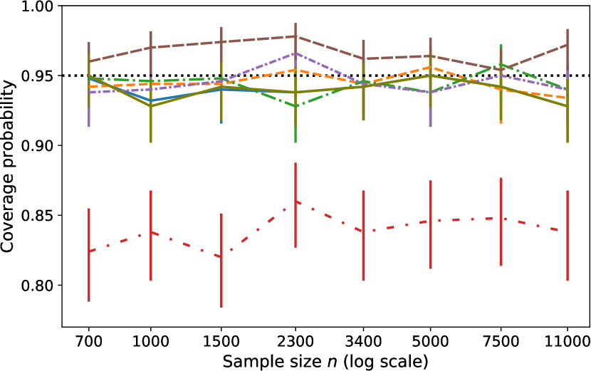
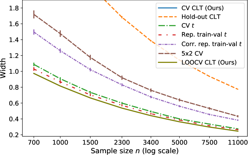
Figure 3: Test error coverage (left) and width (right) of $95\%$ confidence intervals for ridge regression, including leave-one-out CV intervals (see Sec. 5.4). The CV CLT curves are obscured by the nearly identical LOOCV CLT curves.

Efficient computation

We explain here how the Sherman–Morrison–Woodbury formula can be used to efficiently compute the individual losses $h_{n}(Z_{i},Z_{\{i\}^{c}})$, and therefore $\hat{R}_{n}$ as well as $\hat{\sigma}_{n,out}$, and the loss on the instances used to form a surrogate ground-truth estimate of the target error $R_{n}$. Let $X\in\mathbb{R}^{n\times p}$ be the matrix of predictors, whose $i$-th row is $x_{i}^{\top}$, and $Y\in\mathbb{R}^{n}$ be the target variable. The weight vector estimate $\hat{w}$ minimizes $\min_{w\in\mathbb{R}^{p}}\|Y-Xw\|_{2}^{2}+\lambda\|w\|_{2}^{2}$, and is given by the closed-form formula

$$\textstyle\hat{w}=(X^{\top}X+\lambda I_{p})^{-1}X^{\top}Y.$$ (K.1)

We precompute $M\triangleq(X^{\top}X+\lambda I_{p})^{-1}$ and $v\triangleq X^{\top}Y$, that satisfy $\hat{w}=Mv$. Suppose that we have an additional set with covariate matrix $\tilde{X}$ and target variable $\tilde{Y}$, representing the instances used to form a surrogate ground-truth estimate of $R_{n}$. We also precompute $q\triangleq\tilde{X}\hat{w}$ and $A\triangleq\tilde{X}M$.

For the datapoint $i$, let $X^{(-i)}$ denote $X$ without its $i$-th row and $Y^{(-i)}$ denote $Y$ without its $i$-th element. Let $M_{i}\triangleq({X^{(-i)}}^{\top}X^{(-i)}+\lambda I_{p})^{-1}$, $v_{i}\triangleq{X^{(-i)}}^{\top}Y^{(-i)}$ and $w_{i}\triangleq M_{i}v_{i}$. We can efficiently compute $M_{i}$ from $M$ based on the Sherman–Morrison–Woodbury formula.

$$\textstyle M_{i} \textstyle=({X^{(-i)}}^{\top}X^{(-i)}+\lambda I_{p})^{-1}$$ (K.2)

$$\textstyle=(X^{\top}X-x_{i}x_{i}^{\top}+\lambda I_{p})^{-1}$$ (K.3)

$$\textstyle=M-Mx_{i}x_{i}^{\top}M/(-1+h_{i}),$$ (K.4)

where $h_{i}\triangleq x_{i}^{\top}Mx_{i}$.

We can compute $v_{i}$ from $v$, with $v_{i}={X^{(-i)}}^{\top}Y^{(-i)}=v-x_{i}y_{i}$.

Therefore, $w_{i}=M_{i}v_{i}=(M-Mx_{i}x_{i}^{\top}M(-1+h_{i})^{-1})(v-x_{i}y_{i})=\hat{w}+Mx_{i}(\langle\hat{w},x_{i}\rangle-y_{i})/(1-h_{i})$ can be computed without fitting any additional prediction rule. Then $h_{n}(Z_{i},Z_{\{i\}^{c}})=(y_{i}-\langle w_{i},x_{i}\rangle)^{2}$, and we use them to compute $\hat{R}_{n}$ and $\hat{\sigma}_{n,out}$. To make predictions for the covariate matrix $\tilde{X}$, we efficiently compute $\tilde{X}w_{i}$ as

$$\textstyle\tilde{X}w_{i} \textstyle=\tilde{X}\hat{w}+\tilde{X}Mx_{i}(\langle\hat{w},x_{i}\rangle-y_{i})/(1-h_{i})$$ (K.5)

$$\textstyle=q+Ax_{i}(\langle\hat{w},x_{i}\rangle-y_{i})/(1-h_{i}),$$ (K.6)

and $\frac{1}{N}\|\tilde{Y}-\tilde{X}w_{i}\|_{2}^{2}$ is an estimate of $\mathbb{E}[h_{n}(Z_{0},Z_{\{i\}^{c}})\mid Z_{\{i\}^{c}}]$, where $N$ is the size of the whole dataset. An estimate of $R_{n}$ is then $\frac{1}{n}\sum_{i=1}^{n}\frac{1}{N}\|\tilde{Y}-\tilde{X}w_{i}\|_{2}^{2}$.

Appendix L Additional Experimental Results

This section reports the additional results of the experiments described in Sec. 5.

L.1 Additional results from Sec. 5.1: Confidence intervals for test error

The remaining results of the experiments described in Sec. 5.1 are provided in Figs. 4 and 5. We remind that each mean width estimate is displayed with a $\pm$ 2 standard error confidence band, while the confidence band surrounding each coverage estimate is a 95% Wilson interval. For all $6$ learning tasks, all procedures except the repeated train-validation $t$ interval provide near-nominal coverage, and our CV CLT intervals provide the smallest widths.

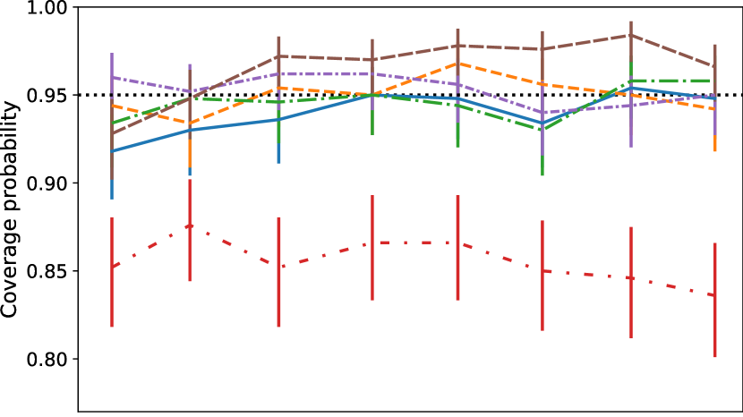
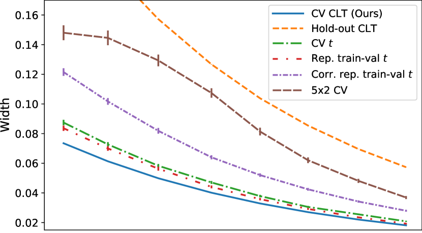
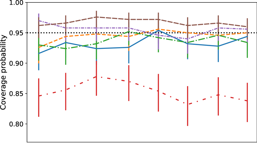
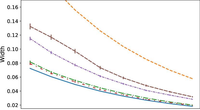
Figure 4: Test error coverage (left) and width (right) of $95\%$ confidence intervals (see Sec. 5.1). Top: $\ell^{2}$-regularized logistic regression classifier. Middle: Random forest classifier. Bottom: Neural network classifier.

L.2 Additional results from Sec. 5.2: Testing for improved algorithm performance

In this section, we provide additional experimental details and results for the testing for improved algorithm performance experiments of Sec. 5.2. We highlight that the aim of this assessment is not to establish power convergence or to assess power in an absolute sense but rather to verify whether, for a diversity of settings encountered in real learning problems, our proposed tests provide power comparable to or better than the most popular heuristics from the literature. For all testing experiments, we estimate size as $\frac{\text{\# of rejections in }H_{0}\text{ replications}}{\text{\# }H_{0}\text{ replications}}$ and power as $\frac{\text{\# of rejections in }H_{1}\text{ replications}}{\text{\# }H_{1}\text{ replications}}$, where each simulation is classified as $H_{0}$ or $H_{1}$ depending on which algorithm has smaller test error. Moreover, a size point is only displayed if at least 25 replications were classified as $H_{0}$, and a power point is only displayed if at least 25 replications were classified as $H_{1}$.

The remaining results of the testing experiments described in Sec. 5.2 are provided in Figs. 11, 7, 6, 8, 10 and 9. In contrast to Fig. 2, in Figs. 11, 7, 6, 8, 10 and 9 we plot the size and power of the level $\alpha=0.05$ test of $H_{1}:\text{Err}(\mathcal{A}_{1})<\text{Err}(\mathcal{A}_{2})$ in the left column of each figure and the size and power of the level $\alpha$ test of $H_{1}:\text{Err}(\mathcal{A}_{2})<\text{Err}(\mathcal{A}_{1})$ in the right column. Notably, we only observe size estimates exceeding the level when the number of $H_{0}$ replications is very small (that is, when one algorithm improves upon the other so infrequently that the Monte Carlo error in the size estimate is large).

L.3 Testing with synthetically generated labels

We complement the real-data hypothesis testing experiments of Sec. 5.2 with a controlled experiment in which class labels are synthetically generated from a known logistic regression distribution. Specifically, we replicate the exact classification experimental setup of Sec. 5.2 to compare logistic regression and random forest classification and use the same Higgs dataset covariates, but we replace each datapoint label $Y_{i}$ with an independent draw from the logistic regression distribution $Y_{i}\sim\textnormal{Ber}(\frac{1}{1+\exp({-\langle{X_{i}},{\beta}\rangle})})$ for $\beta$ a 28-dimensional vector with odd entries equal to $1$ and even entries equal to $-1$. This experiment enables us to evaluate our hypothesis tests in a realizable setting in which the true label generating distribution belongs to the logistic regression model family. In Fig. 12, we plot in the left column the size and power of the level $\alpha=0.05$ test of $H_{1}$: random forest improves upon $\ell^{2}$-regularized logistic regression classifier, and in the right column the size and power of the level $\alpha$ test of $H_{1}$: $\ell^{2}$-regularized logistic regression classifier improves upon random forest. As expected, almost all replications satisfy that $\ell^{2}$-regularized logistic regression improves upon random forest and we observe that in this setting as well, our method consistently outperforms other alternatives.

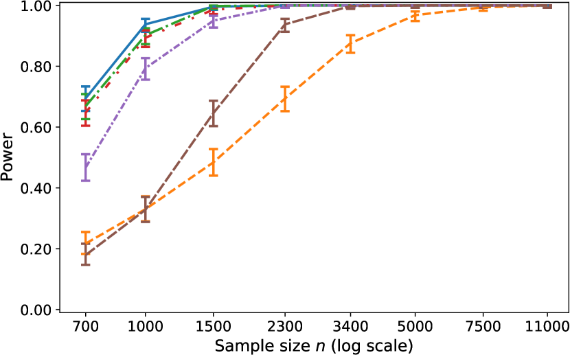
Figure 6: Size (top) and power (bottom) of level-$0.05$ tests for improved test error (see Sec. 5.2). Left: Testing $H_{1}$: neural network improves upon $\ell^{2}$-regularized logistic regression classifier. Right: Testing $H_{1}$: $\ell^{2}$-regularized logistic regression classifier improves upon neural network.

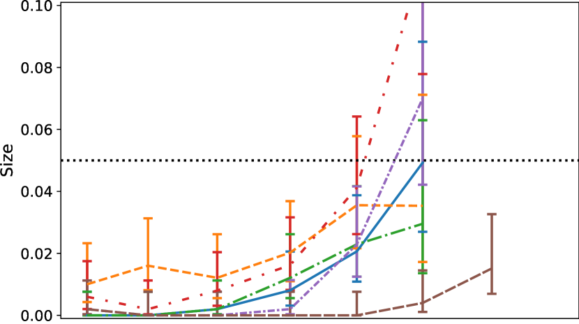
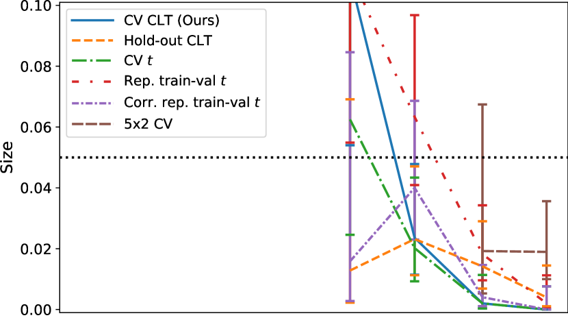
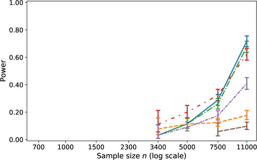
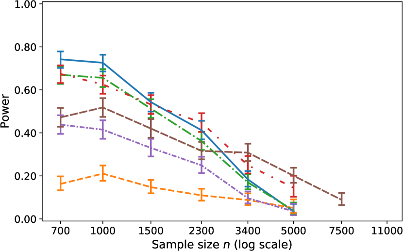
Figure 7: Size (top) and power (bottom) of level-$0.05$ tests for improved test error (see Sec. 5.2). Left: Testing $H_{1}$: $\ell^{2}$-regularized logistic regression classifier improves upon random forest. Right: Testing $H_{1}$: random forest improves upon $\ell^{2}$-regularized logistic regression classifier.

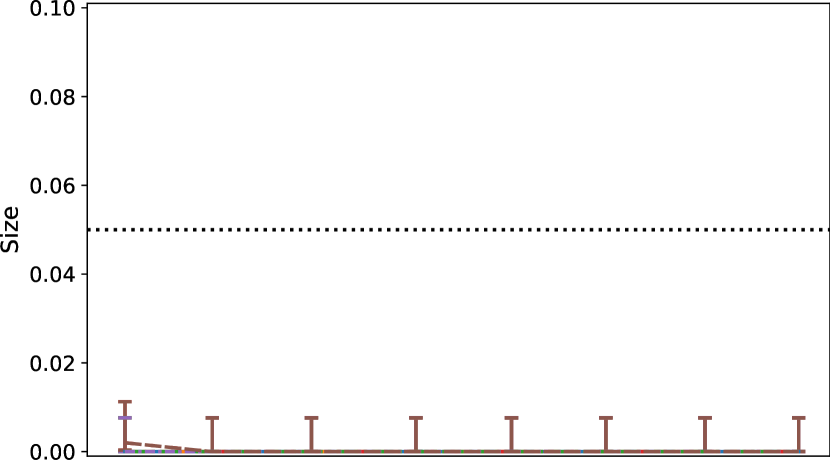
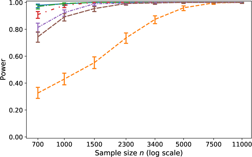
Figure 8: Size (top) and power (bottom) of level-$0.05$ tests for improved test error (see Sec. 5.2). Left: Testing $H_{1}$: neural network classifier improves upon random forest. Right: Testing $H_{1}$: random forest classifier improves upon neural network.

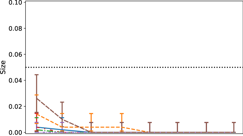
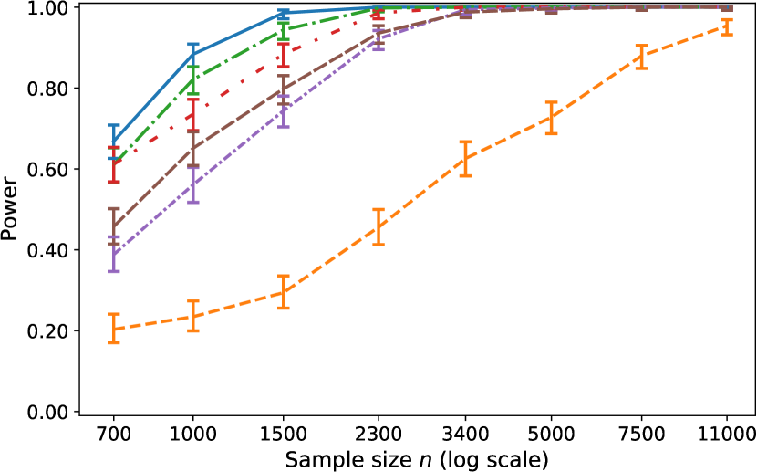
Figure 9: Size (top) and power (bottom) of level-$0.05$ tests for improved test error (see Sec. 5.2). Left: Testing $H_{1}$: ridge regression improves upon random forest. Right: Testing $H_{1}$: random forest improves upon ridge regression.

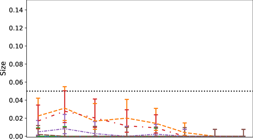
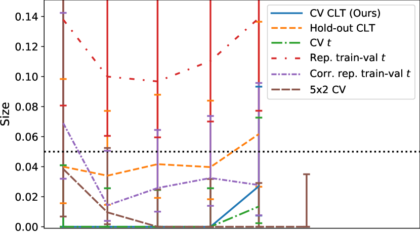
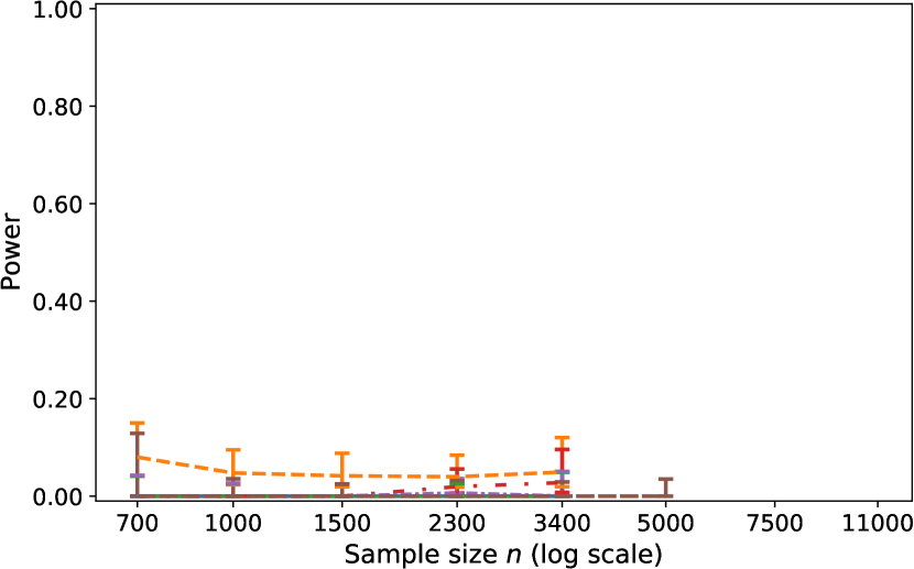
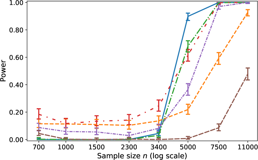
Figure 10: Size (top) and power (bottom) of level-$0.05$ tests for improved test error (see Sec. 5.2). Left: Testing $H_{1}$: neural network improves upon ridge regression. Right: Testing $H_{1}$: ridge regression improves upon neural network.

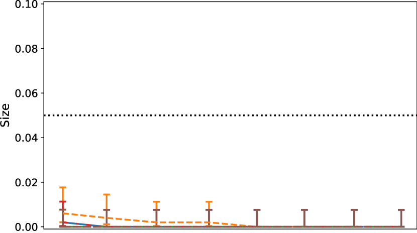
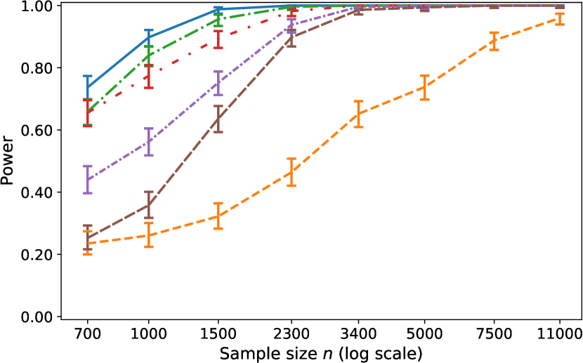
Figure 11: Size (top) and power (bottom) of level-$0.05$ tests for improved test error (see Sec. 5.2). Left: Testing $H_{1}$: neural network regression improves upon random forest. Right: Testing $H_{1}$: random forest regression improves upon neural network.

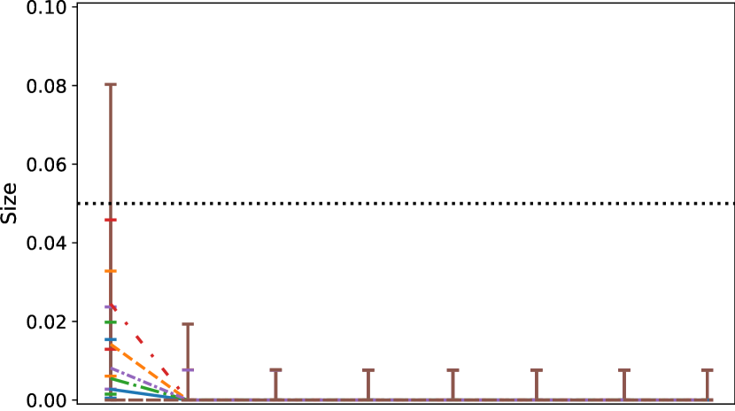
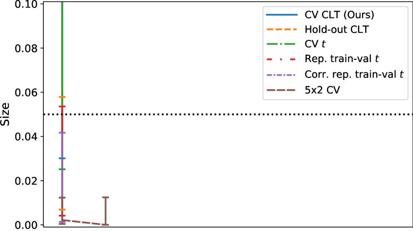
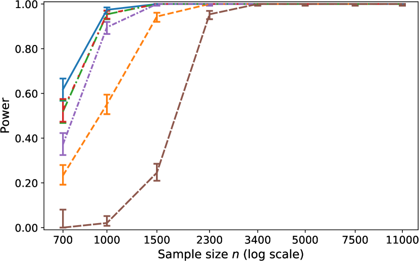
Figure 12: Size (top) and power (bottom) of level-$0.05$ tests for improved test error with synthetic logistic regression labels (see Sec. L.3). Left: Testing $H_{1}$: random forest improves upon $\ell^{2}$-regularized logistic regression classifier. Right: Testing $H_{1}$: $\ell^{2}$-regularized logistic regression classifier improves upon random forest.

L.4 Results for Sec. 5.3: Importance of stability

In this section, we provide the figures (Figs. 13, 14 and 15) and experimental details supporting the importance of stability experiment of Sec. 5.3. Compared to the chosen hyperparameters described in App. K, for this example, we used the default value of max_depth for XGBRFRegressor, that is 6, and the default value of alpha for MLPRegressor, that is 1e-4. For Figs. 15(a) and 15(b), we obtain an estimate of $\sigma_{n}^{2}=\mathrm{Var}(\bar{h}_{n}(Z_{0}))$ by computing a Monte Carlo approximation of $\bar{h}_{n}(Z_{0})=\mathbb{E}[h_{n}(Z_{0},Z_{1:m})\mid Z_{0}]$ for each of 10,000 $Z_{0}$ values and then reporting the empirical variance of these 10,000 approximated values. For each value of $Z_{0}$ we employ the Monte Carlo approximation of

$$\bar{h}_{n}(Z_{0})\approx\frac{1}{500}\sum_{\ell=1}^{500}\frac{1}{k}\sum_{j=1}^{k}h_{n}(Z_{0},Z^{(\ell)}_{B_{j}})$$ (L.1)

where $(Z_{1:n}^{(\ell)})_{\ell=1}^{500}$ are the $500$ datasets of size $n$ described in App. K.

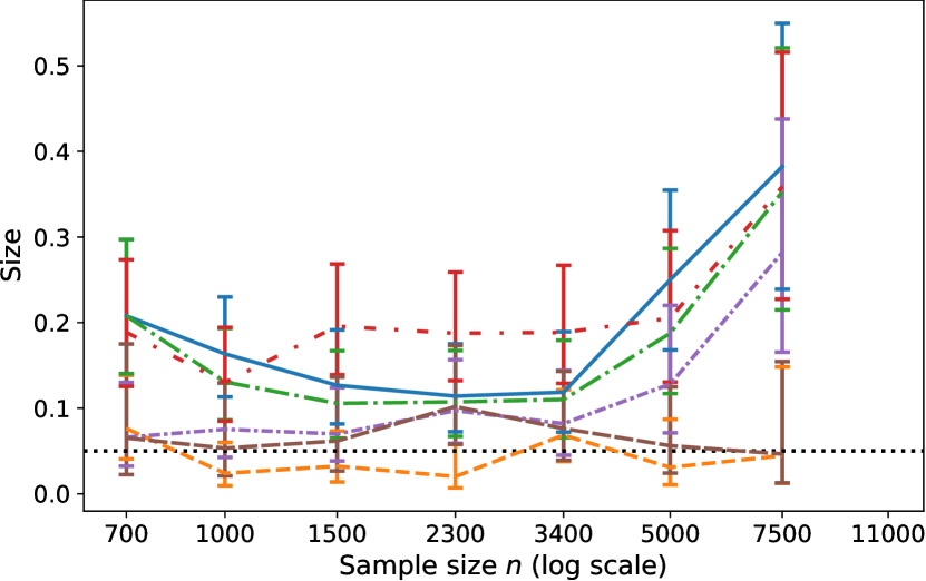
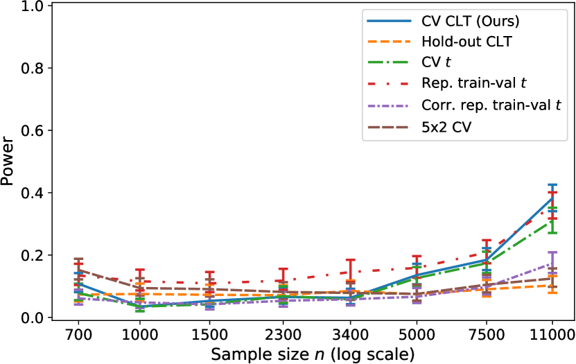
Figure 13: Impact of instability on size (left) and power (right) of level-$0.05$ tests for improved test error (see Sec. 5.3). Testing $H_{1}$: less stable neural network regression improves upon less stable random forest.

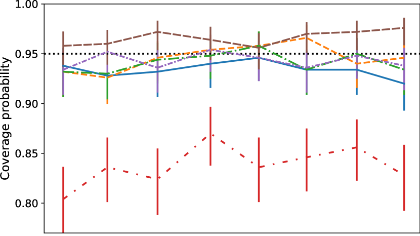
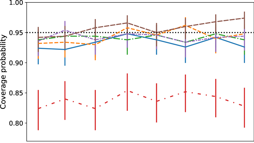
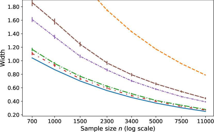
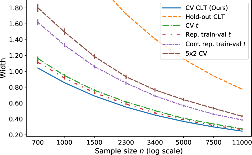
Figure 14: Impact of instability on test error coverage (top) and width (bottom) of $95\%$ confidence intervals (see Sec. 5.3). Left: Less stable neural network regression. Right: Less stable random forest regression.

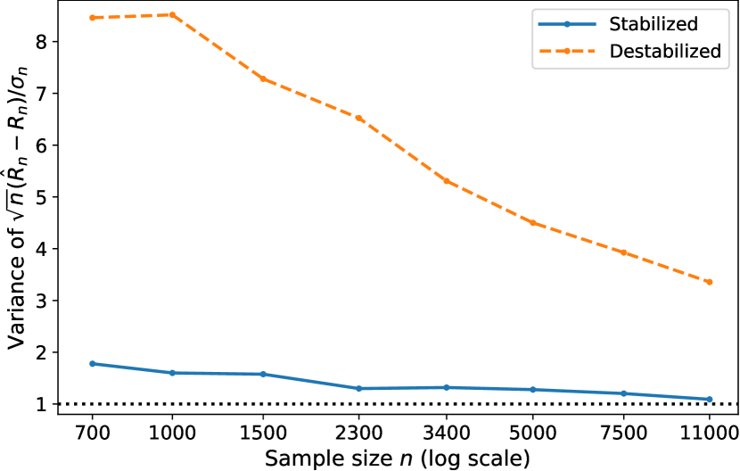
(a) Algorithm comparison

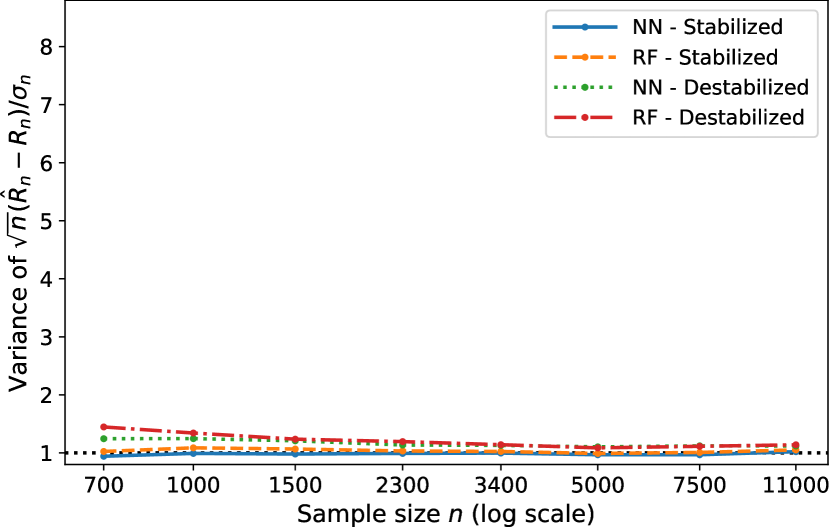
(b) Single algorithm assessment

Figure 15: Impact of instability on variance of $\frac{\sqrt{n}}{\sigma_{n}}(\hat{R}_{n}-R_{n})$ (see Sec. 5.3). Left: $h_{n}(Z_{0},Z_{B})=(Y_{0}-\hat{f}_{1}(X_{0};Z_{B}))^{2}-(Y_{0}-\hat{f}_{2}(X_{0};Z_{B}))^{2}$ for neural network and random forest prediction rules, $\hat{f_{1}}$ and $\hat{f_{2}}$. As predicted in Thms. 1 and 2, the variance is close to $1$ when $h_{n}$ is stable, but the variance can be much larger when $h_{n}$ is unstable. Right: $h_{n}(Z_{0},Z_{B})=(Y_{0}-\hat{f}(X_{0};Z_{B}))^{2}$ for neural network or random forest prediction rule, $\hat{f}$. The same destabilized algorithms produce relatively stable $h_{n}$ in the context of single algorithm assessment, as the variance parameter $\sigma_{n}^{2}=\mathrm{Var}(\bar{h}_{n}(Z_{0}))$ is larger.

References

- dat, [2015] (2015). FlightDelays dataset. https://www.kaggle.com/usdot/flight-delays.
- [2] Abou-Moustafa, K. and Szepesvári, C. (2019a). An exponential tail bound for Lq stable learning rules. In Garivier, A. and Kale, S., editors, Proceedings of the 30th International Conference on Algorithmic Learning Theory, volume 98 of Proceedings of Machine Learning Research, pages 31–63, Chicago, Illinois. PMLR.
- [3] Abou-Moustafa, K. and Szepesvári, C. (2019b). An exponential tail bound for the deleted estimate. In Proceedings of the Thirty-Third AAAI Conference on Artificial Intelligence, pages 42–50.
- Arsov et al., [2019] Arsov, N., Pavlovski, M., and Kocarev, L. (2019). Stability of decision trees and logistic regression. arXiv preprint arXiv:1903.00816v1.
- Austern and Zhou, [2020] Austern, M. and Zhou, W. (2020). Asymptotics of Cross-Validation. arXiv preprint arXiv:2001.11111v2.
- [6] Baldi, P., Sadowski, P., and Whiteson, D. (2014a). Searching for exotic particles in high-energy physics with deep learning. Nature Communications, 5.
- [7] Baldi, P., Sadowski, P., and Whiteson, D. (2014b). Higgs dataset. https://archive.ics.uci.edu/ml/datasets/HIGGS.
- Beirami et al., [2017] Beirami, A., Razaviyayn, M., Shahrampour, S., and Tarokh, V. (2017). On optimal generalizability in parametric learning. In Proceedings of the 31st International Conference on Neural Information Processing Systems, NIPS’17, pages 3455–3465, Red Hook, NY, USA. Curran Associates Inc.
- Bengio and Grandvalet, [2004] Bengio, Y. and Grandvalet, Y. (2004). No unbiased estimator of the variance of -fold cross validation. Journal of Machine Learning Research, 5:1089–1105.
- Billingsley, [1995] Billingsley, P. (1995). Probability and Measure, Third Edition.
- Blum et al., [1999] Blum, A., Kalai, A., and Langford, J. (1999). Beating the hold-out: Bounds for -fold and progressive cross-validation. In Proc. COLT, pages 203–208.
- Boucheron et al., [2005] Boucheron, S., Bousquet, O., Lugosi, G., and Massart, P. (2005). Moment inequalities for functions of independent random variables. Annals of Probability, 33(2):514–560.
- Bouckaert and Frank, [2004] Bouckaert, R. R. and Frank, E. (2004). Evaluating the replicability of significance tests for comparing learning algorithms. In PAKDD, pages 3–12. Springer.
- Bousquet and Elisseeff, [2002] Bousquet, O. and Elisseeff, A. (2002). Stability and generalization. Journal of Machine Learning Research, 2:499–526.
- Brown et al., [2001] Brown, L. D., Cai, T. T., and DasGupta, A. (2001). Interval estimation for a binomial proportion. Statistical Science, 16(2):101–133.
- Celisse and Guedj, [2016] Celisse, A. and Guedj, B. (2016). Stability revisited: new generalisation bounds for the Leave-one-Out. arXiv preprint arXiv:1608.06412v1.
- Chen and Guestrin, [2016] Chen, T. and Guestrin, C. (2016). Xgboost: A scalable tree boosting system. In Proceedings of the 22nd ACM SIGKDD International Conference on Knowledge Discovery and Data Mining, KDD ’16, pages 785–794, New York, NY, USA. Association for Computing Machinery.
- Cornec, [2010] Cornec, M. (2010). Concentration inequalities of the cross-validation estimate for stable predictors. arXiv preprint arXiv:1011.5133v1.
- Demšar, [2006] Demšar, J. (2006). Statistical comparisons of classifiers over multiple data sets. Journal of Machine Learning Research, 7:1–30.
- [20] Devroye, L. and Wagner, T. (1979a). Distribution-free inequalities for the deleted and holdout error estimates. IEEE Transactions on Information Theory, 25(2):202–207.
- [21] Devroye, L. and Wagner, T. (1979b). Distribution-free performance bounds for potential function rules. IEEE Transactions on Information Theory, 25(5):601–604.
- Dietterich, [1998] Dietterich, T. G. (1998). Approximate statistical tests for comparing supervised classification learning algorithms. Neural Computation, 10(7):1895–1923.
- Dudoit and van der Laan, [2005] Dudoit, S. and van der Laan, M. J. (2005). Asymptotics of cross-validated risk estimation in estimator selection and performance assessment. Statistical Methodology, 2(2):131–154.
- Durrett, [2019] Durrett, R. (2019). Probability: Theory and Examples, Version 5.
- Elisseeff et al., [2005] Elisseeff, A., Evgeniou, T., and Pontil, M. (2005). Stability of randomized learning algorithms. Journal of Machine Learning Research, 6:55–79.
- Geisser, [1975] Geisser, S. (1975). The predictive sample reuse method with applications. Journal of the American Statistical Association, 70(350):320–328.
- Ghosh et al., [2020] Ghosh, S., Stephenson, W. T., Nguyen, T. D., Deshpande, S. K., and Broderick, T. (2020). Approximate Cross-Validation for Structured Models. arXiv preprint arXiv:2006.12669v1.
- Giordano et al., [2019] Giordano, R., Stephenson, W., Liu, R., Jordan, M., and Broderick, T. (2019). A swiss army infinitesimal jackknife. In Chaudhuri, K. and Sugiyama, M., editors, Proceedings of Machine Learning Research, volume 89 of Proceedings of Machine Learning Research, pages 1139–1147. PMLR.
- Hardt et al., [2016] Hardt, M., Recht, B., and Singer, Y. (2016). Train faster, generalize better: Stability of stochastic gradient descent. In Proceedings of the 33rd International Conference on Machine Learning - Volume 48, ICML’16, pages 1225–1234. JMLR.org.
- Jiang et al., [2008] Jiang, W., Varma, S., and Simon, R. (2008). Calculating Confidence Intervals for Prediction Error in Microarray Classification Using Resampling. Statistical Applications in Genetics and Molecular Biology, 7(1).
- Kale et al., [2011] Kale, S., Kumar, R., and Vassilvitskii, S. (2011). Cross-validation and mean-square stability. In Proceedings of the Second Symposium on Innovations in Computer Science (ICS2011). Citeseer.
- Kearns and Ron, [1999] Kearns, M. and Ron, D. (1999). Algorithmic stability and sanity-check bounds for leave-one-out cross-validation. Neural Computation, 11(6):1427–1453.
- Koh et al., [2019] Koh, P. W., Ang, K.-S., Teo, H. H. K., and Liang, P. (2019). On the Accuracy of Influence Functions for Measuring Group Effects. In Proceedings of the 32nd International Conference on Neural Information Processing Systems, NIPS’19, pages 5254–5264.
- Kumar et al., [2013] Kumar, R., Lokshtanov, D., Vassilvitskii, S., and Vattani, A. (2013). Near-optimal bounds for cross-validation via loss stability. In International Conference on Machine Learning, pages 27–35.
- Kutin and Niyogi, [2002] Kutin, S. and Niyogi, P. (2002). Almost-everywhere algorithmic stability and generalization error. In Proceedings of the Eighteenth Conference on Uncertainty in Artificial Intelligence, UAI’02, pages 275–282, San Francisco, CA, USA. Morgan Kaufmann Publishers Inc.
- LeDell et al., [2015] LeDell, E., Petersen, M., and van der Laan, M. (2015). Computationally efficient confidence intervals for cross-validated area under the roc curve estimates. Electronic Journal of Statistics, 9(1):1583–1607.
- Lei, [2019] Lei, J. (2019). Cross-validation with confidence. Journal of the American Statistical Association, pages 1–20.
- Lim et al., [2000] Lim, T.-S., Loh, W.-Y., and Shih, Y.-S. (2000). A comparison of prediction accuracy, complexity, and training time of thirty-three old and new classification algorithms. Mach. Learn., 40(3):203–228.
- Markatou et al., [2005] Markatou, M., Tian, H., Biswas, S., and Hripcsak, G. (2005). Analysis of variance of cross-validation estimators of the generalization error. Journal of Machine Learning Research, 6:1127–1168.
- McNemar, [1947] McNemar, Q. (1947). Note on the sampling error of the difference between correlated proportions or percentages. Psychometrika, 12:153–157.
- Meyer, [1966] Meyer, P.-A. (1966). Probability and Potentials. Blaisdell Publishing Co, N.Y.
- Michiels et al., [2005] Michiels, S., Koscielny, S., and Hill, C. (2005). Prediction of cancer outcome with microarrays: a multiple random validation strategy. The Lancet, 365(9458):488–492.
- Nadeau and Bengio, [2003] Nadeau, C. and Bengio, Y. (2003). Inference for the generalization error. Machine Learning, 52(3):239–281.
- Pedregosa et al., [2011] Pedregosa, F., Varoquaux, G., Gramfort, A., Michel, V., Thirion, B., Grisel, O., Blondel, M., Prettenhofer, P., Weiss, R., Dubourg, V., Vanderplas, J., Passos, A., Cournapeau, D., Brucher, M., Perrot, M., and Duchesnay, E. (2011). Scikit-learn: Machine learning in Python. Journal of Machine Learning Research, 12:2825–2830.
- Pirracchio et al., [2015] Pirracchio, R., Petersen, M. L., Carone, M., Rigon, M. R., Chevret, S., and van der Laan, M. J. (2015). Mortality prediction in intensive care units with the Super ICU Learner Algorithm (SICULA): a population-based study. The Lancet Respiratory Medicine, 3(1):42–52.
- Rad and Maleki, [2020] Rad, K. R. and Maleki, A. (2020). A scalable estimate of the out-of-sample prediction error via approximate leave-one-out cross-validation. Journal of the Royal Statistical Society: Series B (Statistical Methodology).
- Steele, [1986] Steele, J. M. (1986). An Efron-Stein inequality for nonsymmetric statistics. Annals of Statistics, 14(2):753–758.
- Stephenson and Broderick, [2020] Stephenson, W. and Broderick, T. (2020). Approximate cross-validation in high dimensions with guarantees. In Chiappa, S. and Calandra, R., editors, Proceedings of the Twenty Third International Conference on Artificial Intelligence and Statistics, volume 108 of Proceedings of Machine Learning Research, pages 2424–2434, Online. PMLR.
- Stone, [1974] Stone, M. (1974). Cross-validatory choice and assessment of statistical predictions. Journal of the Royal Statistical Society. Series B (Methodological), 36(2):111–147.
- Wilson et al., [2020] Wilson, A., Kasy, M., and Mackey, L. (2020). Approximate cross-validation: Guarantees for model assessment and selection. In Chiappa, S. and Calandra, R., editors, Proceedings of the Twenty Third International Conference on Artificial Intelligence and Statistics, volume 108 of Proceedings of Machine Learning Research, pages 4530–4540, Online. PMLR.
- Wilson, [1927] Wilson, E. B. (1927). Probable inference, the law of succession, and statistical inference. Journal of the American Statistical Association, 22(158):209–212.