Deep Co-Training with Task Decomposition
for Semi-Supervised Domain Adaptation

Abstract

Semi-supervised domain adaptation (SSDA) aims to adapt models trained from a labeled source domain to a different but related target domain, from which unlabeled data and a small set of labeled data are provided. Current methods that treat source and target supervision without distinction overlook their inherent discrepancy, resulting in a source-dominated model that has not effectively use the target supervision. In this paper, we argue that the labeled target data needs to be distinguished for effective SSDA, and propose to explicitly decompose the SSDA task into two sub-tasks: a semi-supervised learning (SSL) task in the target domain and an unsupervised domain adaptation (UDA) task across domains. By doing so, the two sub-tasks can better leverage the corresponding supervision and thus yield very different classifiers. To integrate the strengths of the two classifiers, we apply the well established co-training framework, in which the two classifiers exchange their high confident predictions to iteratively “teach each other” so that both classifiers can excel in the target domain. We call our approach Deep Co-training with Task decomposition (DeCoTa). DeCoTa requires no adversarial training and is easy to implement. Moreover, DeCoTa is well founded on the theoretical condition of when co-training would succeed. As a result, DeCoTa achieves state-of-the-art results on several SSDA datasets, outperforming the prior art by a notable $4\%$ margin on DomainNet. Code is available at https://github.com/LoyoYang/DeCoTa.

1 Introduction

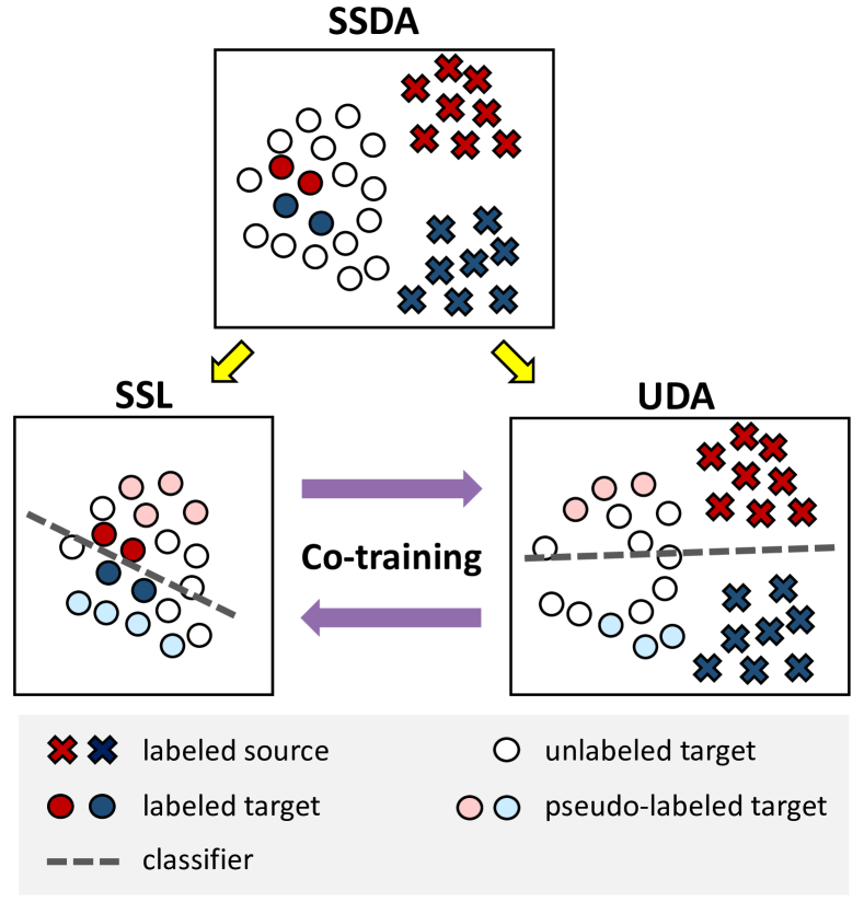
Figure 1: Deep Co-training with Task decomposition (DeCoTa). We decompose semi-supervised domain adaptation (SSDA) into two sub-tasks: semi-supervised learning (SSL) in the target domain, and unsupervised DA (UDA) across domains. The two sub-tasks offer different pseudo-label confidences to the unlabeled data (light blue & light red circles), which we leverage via co-training: exchanging their high confident predictions to teach each other.

Domain adaptation (DA) aims to adapt machine learned models from a source domain to a related but different target domain [4, 14, 53, 13]. DA is particularly important in settings where labeled target data is hard to obtain, but labeled source data is plentiful [63, 41, 21], e.g., adaptation from synthetic to real images [21, 55, 48, 47, 56] and adaptation to a new or rare environment [10, 69, 54, 9]. Most of the existing works focus on the unsupervised domain adaptation (UDA) setting, in which the target domain is completely unlabeled. Several recent works, however, show that adding merely a tiny amount of target labeled data (e.g., just one labeled image per class) can notably boost the performance [51, 26, 45, 1, 31, 30, 12, 74], suggesting that this setting may be more promising for domain adaptation to succeed. In this paper, we thus focus on the latter setting, which is referred to as semi-supervised domain adaptation (SSDA).

Despite the seemingly nuanced difference between the two settings, methods that are effective for SSDA and UDA can vary substantially. For instance, [51] showed that directly combining the labeled source and labeled target data and then applying popular UDA algorithms like domain adversarial learning [13] or entropy minimization [16] can hardly improve the performance. In other words, the labeled target data have not been effectively used. Existing methods [51, 45, 26] therefore propose additional objectives to strengthen the influence of labeled target data in SSDA.

Intrigued by these findings, we investigate the characteristics of SSDA further and emphasize two fundamental challenges. First, the amount of labeled source data is much larger than that of labeled target data. Second, the two data are inherently different in their distributions. A single classifier learned together with both sources of supervision is thus easily dominated by the labeled source data and is unable to take advantage of the additional labeled target data.

To resolve this issue, we propose to explicitly decompose the two sources of supervision and learn two distinct classifiers whose goals are however shared: to classify well on the unlabeled target data. To this end, we pair the labeled source data and the unlabeled target data to learn one classifier, which is essentially a UDA task. For the other classifier, we pair the labeled and unlabeled target data, which is essentially a semi-supervised learning (SSL) task. That is, we explicitly decompose SSDA into two well-studied tasks.

For each sub-task, one may apply any existing algorithms independently. In this paper, we however investigate the idea of learning the two classifiers jointly for two compelling reasons. First, the two tasks share the same goal and same unlabeled data, meaning that they are correlated. Second, learning with distinct labeled data implies that the two classifiers will converge differently in what types of mistakes they make and on which samples they are confident and correct, meaning that they are complementary to each other.

We therefore propose to learn the two classifiers jointly via co-training [6, 2, 8], which is arguably one of the most established algorithm for learning with multi views: in our case, two correlating and complementary tasks. The approach is straightforward: train a separate classifier on each task using its labeled data, and use them to create pseudo-labels for the unlabeled data. As the two classifiers are trained with distinct supervision, they will yield different predictions. In particular, there will be samples that only one classifier is confident about (and more likely to be correct). By labeling these samples with the confident classifier’s predictions and adding them to the training set of the other classifier to re-train on, the two classifiers are essentially “teaching each other” to improve. To this end, we employ a simple pseudo-labeling-based algorithm with deep learning, similar to [5], to train each classifier. Pseudo-labeling-based algorithms have been shown powerful for both the UDA and SSL tasks [70, 27]. In other words, we can apply the same algorithm for both sub-tasks, greatly simplifying our overall framework which we name DeCoTa: Deep Co-training with Task Decomposition (Fig. 1 gives an illustration).

We evaluate DeCoTa on two benchmark datasets for SSDA: DomainNet [41] and Office-home [66]. While very simple to implement and without any adversarial training [51, 45], DeCoTa significantly outperforms the state-of-the-art results [45, 26] on DomainNet by over $4\%$ and is on a par with them on Office-home. We attribute this to the empirical evidence that our task decomposition fits the theoretical condition of relaxed $\epsilon$-expandability [8, 2], which is sufficient for co-training to succeed. Another strength of DeCoTa is that it requires no extra learning process like feature decomposition to create views from data [8, 44, 7]. To the best of our knowledge, our paper is the first to enable deep learning with co-training on SSDA.

The contributions of this work are as follow. (1) We explicitly decompose the two very different sources of supervision, labeled source and labeled target data, in SSDA. (2) We present DeCoTa, a simple deep learning based co-training approach for SSDA to jointly learn two classifiers, one for each supervision. (3) we provide intermediate results and insights that illustrate why DeCoTa works. Specifically, we show that DeCoTa satisfies the $\epsilon$-expandability requirement [2] of co-training. (4) Lastly, we support this work with strong empirical results that outperform state-of-the-art.

2 Related Work

Unsupervised domain adaptation (UDA). UDA has been studied extensively. Many methods [33, 57, 65] matched the feature distributions between domains by minimizing their divergence. One mainstream approach is by domain adversarial learning [13, 21, 68, 40, 67, 71, 69, 73]. More recent works [52, 53, 29, 57] learn features based on the cluster assumption [16]: classifier boundaries should not cross high density target data regions. For example, [52, 53] attempted to push target features away from the boundary, using minmax training. Some other approaches employ self-training with pseudo-labeling [28, 37, 38, 3] to progressively label unlabeled data and use them to fine-tune the model [7, 25, 78, 24, 62, 32, 23, 27]. A few recent methods use MixUp [76], but mainly to augment adversarial learning based UDA approaches (e.g., [13]) by stabilizing the domain discriminator [61, 71] or smoothing the predictions [36, 72]. In contrast, we apply MixUp to create better pseudo-labeled data for co-training, without adversarial learning.

Semi-supervised domain learning (SSDA). SSDA attracts less attention in DA, despite its promising scenario in balancing accuracy and labeling effort. With few labeled target data, SSDA can quickly reshape the class boundaries to boost the accuracy [51, 45]. Many SSDA works are proposed prior to deep learning [74, 31, 20, 42], matching features while maintaining accuracy on labeled target data. [1, 64] employed knowledge distillation [19] to regularize the training on labeled target data. More recent works use deep learning, and find that the popular UDA principle of aligning feature distributions could fail to learn discriminative class boundaries in SSDA [51]. [51] thus proposed to gradually move the class prototypes (used to derive class boundaries) to the target domain in a minimax fashion; [45] introduced opposite structure learning to cluster target data and scatter source data to smooth the process of learning class boundaries. Both works [45, 51] and [26] concatenate the target labeled data with the source data to expand the labeled data. [30] incorporates meta-learning to search for better initial condition in domain adaptation. SSDA is also related to [60, 43], in which active learning is incorporated to label data for improving domain adaptation.

Co-training. Co-training, a powerful semi-supervised learning (SSL) method proposed in [6], looks at the available data with two views from which two models are trained interactively. By adding the confident predictions of one model to the training set of the other, co-training enables the models to “teach each other”. There were several assumptions to ensure co-training’s effectiveness [6], which were later relaxed by [2] with the notion of $\epsilon$-expandability. [8] broadened the scope of co-training to a single-view setting by learning to decompose a fixed feature representation into two artificially created views; [7] subsequently extended this framework to use co-training for (semi-supervised) domain adaptation. A recent work [44] extended co-training to deep learning models, by encouraging two models to learn different features and behave differently on single-view data. One novelty of DeCoTa is that it works with single-view data (both the UDA and SSL tasks are looking at images) but requires no extra learning process like feature decomposition to artificially create views from such data [8, 44, 7].

Co-training vs. co-teaching. Co-teaching [17] was proposed for learning with noisy data, which shares a similar procedure to co-training by learning two models to filter out noisy data for each other. There are several key differences between them and DeCoTa is based on co-training. As in [17], co-teaching is designed for supervised learning with noisy labels, while co-training is for learning with unlabeled data by leveraging two views. DeCoTa decomposes SSDA into two tasks (two views) to leverage their difference to improve the performance — the core concept of co-training [7]. In contrast, co-teaching does not need two views. Further, co-teaching relies on the memorization of neural nets to select small loss samples to teach the other classifiers, while DeCoTa selects high confident ones from unlabeled data.

3 Deep Co-training with Task Decomposition

3.1 Approach Overview

Co-training strategies have traditionally been applied to data with two views, e.g., audio and video, or webpages with HTML source and link-graph, after which a classifier is trained in each view and they teach each other on the unlabeled data. This is the original formulation from Blum and Mitchell [6], which is later extended to single-view data by [8] for linear models and by [44] for deep neural networks. Both methods require additional objective functions or tasks (e.g., via generating adversarial examples [15]) to learn to create artificial views such that co-training can be applied.

In this paper, we have however discovered that in semi-supervised domain adaptation (SSDA), one can actually conduct co-training using single-view data (all are images) without such an additional learning subroutine. The key is to leverage the inherent discrepancy of the labeled data (i.e., supervision) provided in SSDA: the labeled data from the source domain, $D_{\mathcal{S}}{}=\{(s_{i},y_{i})\}_{i=1}^{N_{S}}$, and the labeled data from the target domain, $D_{\mathcal{T}}{}=\{(t_{i},y_{i})\}_{i=1}^{N_{T}}$, which is usually much smaller than $D_{\mathcal{S}}{}$. By combining each of them with the unlabeled samples from the target domain, $D_{\mathcal{U}}{}=\{u_{i}\}_{i=1}^{N_{U}}$, we can construct two sub-tasks in SSDA:

• an unsupervised domain adaptation (UDA) task that trains a model $\bm{w}_{\color[rgb]{0,0,1}g}$ using $D_{\mathcal{S}}{}$ and $D_{\mathcal{U}}{}$,

• a semi-supervised learning (SSL) task that trains another model $\bm{w}_{\color[rgb]{1,0,0}f}$ using $D_{\mathcal{T}}{}$ and $D_{\mathcal{U}}{}$.

We learn both models by mini-batch stochastic gradient descent (SGD). At every iteration, we sample three data sets, $S=\{(s_{b},y_{b})\}_{b=1}^{B}$ from $D_{\mathcal{S}}{}$, $T=\{(t_{b},y_{b})\}_{b=1}^{B}$ from $D_{\mathcal{T}}{}$, and $U=\{u_{b}\}_{b=1}^{B}$ from $D_{\mathcal{U}}{}$, where $B$ is the mini-batch size. We can then predict on $U$ using the the two models $\bm{w}_{\color[rgb]{0,0,1}g}$ and $\bm{w}_{\color[rgb]{1,0,0}f}$, creating the pseudo-label sets $U^{({\color[rgb]{1,0,0}f})}$ and $U^{({\color[rgb]{0,0,1}g})}$ that will be used to update $\bm{w}_{\color[rgb]{1,0,0}f}$ and $\bm{w}_{\color[rgb]{0,0,1}g}$,

$$U^{({\color[rgb]{1,0,0}f})}= \{(u_{b},\hat{y_{b}}=\operatorname*{arg\,max}_{c}p(c|u_{b};\bm{w}_{\color[rgb]{0,0,1}g}));$$

$$\text{ if }\max_{c}p(c|u_{b};\bm{w}_{\color[rgb]{0,0,1}g})>\tau\},$$

$$U^{(\color[rgb]{0,0,1}g)}= \{(u_{b},\hat{y_{b}}=\operatorname*{arg\,max}_{c}p(c|u_{b};\bm{w}_{{\color[rgb]{1,0,0}f}}));$$

$$\text{ if }\max_{c}p(c|u_{b};\bm{w}_{{\color[rgb]{1,0,0}f}})>\tau\},$$ (1)

where $u_{b}$ is an unlabeled sample drawn from $U$, $p(c|u_{b};\cdot)$ is the predicted probability for a class $c$, and $\tau$ is the threshold for pseudo-label selection. In other words, we use one model’s (say $\bm{w}_{\color[rgb]{0,0,1}g}$) high confident prediction to create pseudo-labels for $u_{b}$, which is then included in $U^{({\color[rgb]{1,0,0}f})}$ that will be used to train the other model $\bm{w}_{{\color[rgb]{1,0,0}f}}$. By looking at $U^{({\color[rgb]{1,0,0}f})}$ and $U^{({\color[rgb]{0,0,1}g})}$ jointly, we are indeed asking one model to simultaneously be a teacher and a student: it provides confident pseudo-labels for the other model to learn from, and learns from the other model’s confident pseudo-labels.

We call this approach DeCoTa, which stands for Deep Co-training with Task Decomposition. In the following, we will discuss how to improve the pseudo-label quality (i.e., its coverage and accuracy) for DeCoTa, and provide in-depth analysis why DeCoTa works.

Input : $\bm{w}_{\color[rgb]{1,0,0}f}$ and $\bm{w}_{\color[rgb]{0,0,1}g}$, learning rate $\eta$, batch size $B$, iteration $N_{\max}$, beta distribution coefficient $\alpha$, confidence threshold $\tau$, data $D_{\mathcal{S}}{}$, $D_{\mathcal{T}}{}$, $D_{\mathcal{U}}{}$;

for $n\leftarrow 1$ to $N_{\max}$ do

       Sample $S=\{(s_{b},y_{b})\}_{b=1}^{B}$ from $D_{\mathcal{S}}{}$,

       Sample $T=\{(t_{b},y_{b})\}_{b=1}^{B}$ from $D_{\mathcal{T}}{}$,

       Sample $U=\{u_{b}\}_{b=1}^{B}$ from $D_{\mathcal{U}}{}$;

       Set $U^{({\color[rgb]{1,0,0}f})}=\emptyset$, $U^{({\color[rgb]{0,0,1}g})}=\emptyset$;

       for $b\leftarrow 1$ to $B$ do

             if $\max_{c}p(c|u_{b};\bm{w}_{\color[rgb]{0,0,1}g})>\tau$ then

                   Update $U^{({\color[rgb]{1,0,0}f})}\leftarrow U^{({\color[rgb]{1,0,0}f})}+\{(u_{b},\hat{y}_{b})\}$, $\hat{y}_{b}=\operatorname*{arg\,max}_{c}p(c|u_{b};\bm{w}_{\color[rgb]{0,0,1}g})$;

             end if

            if $\max_{c}p(c|u_{b};\bm{w}_{\color[rgb]{1,0,0}f})>\tau$ then

                   Update $U^{({\color[rgb]{0,0,1}g})}\leftarrow U^{({\color[rgb]{0,0,1}g})}+\{(u_{b},\hat{y}_{b})\},$ $\hat{y}_{b}=\operatorname*{arg\,max}_{c}p(c|u_{b};\bm{w}_{\color[rgb]{1,0,0}f})$;

             end if

            

       end for

      Obtain $\tilde{U}^{({\color[rgb]{1,0,0}f})}=\{\text{{MixUp}}({U}^{({\color[rgb]{1,0,0}f})}_{i},T_{i};\alpha)\}_{i=1}^{|{U}^{({\color[rgb]{1,0,0}f})}|}$;

       Obtain $\tilde{U}^{({\color[rgb]{0,0,1}g})}=\{\text{{MixUp}}({U}^{({\color[rgb]{0,0,1}g})}_{i},S_{i};\alpha)\}_{i=1}^{|{U}^{({\color[rgb]{0,0,1}g})}|}$;

       Update $\bm{w}_{\color[rgb]{1,0,0}f}\leftarrow\bm{w}_{\color[rgb]{1,0,0}f}-\eta\left(\nabla\mathcal{L}(\bm{w}_{\color[rgb]{1,0,0}f},T)+\nabla\mathcal{L}(\bm{w}_{\color[rgb]{1,0,0}f},\tilde{U}^{({\color[rgb]{1,0,0}f})})\right)$;

       Update $\bm{w}_{\color[rgb]{0,0,1}g}\leftarrow\bm{w}_{\color[rgb]{0,0,1}g}-\eta\left(\nabla\mathcal{L}(\bm{w}_{\color[rgb]{0,0,1}g},S)+\nabla\mathcal{L}(\bm{w}_{\color[rgb]{0,0,1}g},\tilde{U}^{({\color[rgb]{0,0,1}g})})\right)$;

      

end for

Output : $\bm{w}_{f}$ and $\bm{w}_{g}$ (for model ensemble).

Algorithm 1 The DeCoTa algorithm

3.1.1 DeCoTa with High-quality Pseudo-labels

The pseudo-labels acquired from each model are understandably noisy. At the beginning of the training, this problem is especially acute, and affects the efficacy of the model as the training progresses. Our experience shows that mitigation is necessary to handle noise in the pseudo-labels to further enhance DeCoTa, for which we follow recent works of SSL [5] to apply MixUp [76, 35]. MixUp is an operation to construct virtual examples by convex combinations. Given two labeled examples $(x_{1},y_{1})$ and $(x_{2},y_{2})$, we define $\textsc{MixUp}\left((x_{1},y_{1}),(x_{2},y_{2});\alpha\right)$

$$\lambda\sim\text{Beta}(\alpha,\alpha),\hskip 20.0pt$$

$$\tilde{x}=(1-\lambda)x_{1}+\lambda x_{2},\hskip 20.0pt\tilde{y}=(1-\lambda)\bm{e}_{y_{1}}+\lambda\bm{e}_{y_{2}}$$ (2)

to obtain a virtual example $(\tilde{x},\tilde{y})$, where $\bm{e}_{y}$ is a one-hot vector with the $y^{th}$ element being 1. $\lambda$ controls the degree of MixUp while Beta refers to the standard beta distribution.

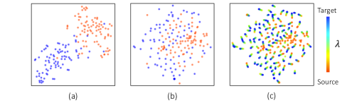
Figure 2: t-SNE visualization of $S$ (red dots, sampled from $D_{\mathcal{S}}{}$) and $U$ (blue dots, sampled from $D_{\mathcal{U}}{}$): (a) before and (b) after including MixUp in calculating the projection; (c) t-SNE of $S$, $U$, and $\textsc{MixUp}(S,U)$. We see a clear data transition along $\lambda$.

We perform MixUp between labeled and pseudo-labeled data: i.e., between samples in $U^{({\color[rgb]{1,0,0}f})}$ and $T$, and between samples in $U^{({\color[rgb]{0,0,1}g})}$ and $S$ to obtain two sets of virtual examples $\tilde{U}^{(f)}$ and $\tilde{U}^{(g)}$. We then update $\bm{w}_{\color[rgb]{1,0,0}f}$ and $\bm{w}_{\color[rgb]{0,0,1}g}$ by SGD,

$$\bm{w}_{\color[rgb]{0,0,1}g}\leftarrow\bm{w}_{\color[rgb]{0,0,1}g}-\eta \left(\nabla\mathcal{L}(\bm{w}_{\color[rgb]{0,0,1}g},S)+\nabla\mathcal{L}(\bm{w}_{\color[rgb]{0,0,1}g},\tilde{U}^{({\color[rgb]{0,0,1}g})})\right),$$ (3)

$$\bm{w}_{\color[rgb]{1,0,0}f}\leftarrow\bm{w}_{\color[rgb]{1,0,0}f}-\eta \left(\nabla\mathcal{L}(\bm{w}_{\color[rgb]{1,0,0}f},T)+\nabla\mathcal{L}(\bm{w}_{\color[rgb]{1,0,0}f},\tilde{U}^{({\color[rgb]{1,0,0}f})})\right),$$

where $\eta$ is the learning rate and $\mathcal{L}$ is the averaged loss over examples. We use the cross-entropy loss.

In our experiments, we have found that MixUp can

• effectively denoise an incorrect pseudo-label by mixing it with a correct one (from $S$ or $T$). The resulting $\tilde{y}$ at least contains a $\lambda$ portion of correct labels;

• smoothly bridge the domain gap between $U$ and $S$. This is done by interpolating between $U^{({\color[rgb]{0,0,1}g})}$ and $S$. The resulting $\tilde{x}$ can be seen as an intermediate example between domains.

In other words, MixUp encourages the models to behave linearly between accurately labeled and pseudo-labeled data, which reduces the undesirable oscillations caused by noisy pseudo-labels and stabilizes the predictions across domains. We note that, our usage of MixUp is fundamentally different from [61, 71, 36, 72] that employed MixUp as auxiliary losses to augment existing DA algorithms like [13].

We illustrate this in  Fig. 2. A model pre-trained on $D_{S}$ is used to generate feature embeddings. We then employ t-SNE [34] to perform two tasks simultaneously, namely clustering the embedded samples as well as projecting them into a 2D space for visualization. In (a), only $S$ sampled from $D_{\mathcal{S}}{}$ and $U$ sampled from $D_{\mathcal{U}}{}$ are embedded, while in (b) and (c), additional samples from MixUp of $S$ and $U$ were added to the fold to influence t-SNE’s clustering step. (b) shows only the finally projected $S$ and $U$ samples afterwards while (c) shows the additional projected MixUp samples as a function of $\lambda$. One can easily see that MixUp effectively closes the gap between the source and target domain. We summarize our proposed algorithm in Algorithm 1.

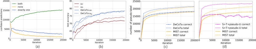
Figure 3: Analysis on the two-task decomposition. We use DomainNet [41] (Real to Clipart; three-shot). (a) We show the number of test examples that both, exactly one, and none of the models have high confidence on (in total, $18,325$). The two tasks hold unique expertise (i.e., there is a $14\%$ portion of the data that exactly one view is confident on), satisfying the condition of co-training in Eq. 6. (b) We show the power of co-training: the same tasks without co-training perform worse, indicating that the models benefit from each other. See Section 3.2 for details. The analysis is on DomainNet (R to C; three-shot) and we will clarify it. We further analyze pseudo-labels in (c) and (d). For every 1K iterations (i.e., 24K unlabeled data with possible repetition), we accumulate the number of data that have confident ($>0.5$) and correct predictions by at least one classifier. See Section 4 for details. (c) Comparison of pseudo-label quantity and quality using DeCoTa vs. MiST. (d) MiST vs. self-training (S+T+pseudo-U). It can be observed that DeCoTa has the largest number of correct pseudo-labels.

3.2 Constraints for Effective Co-training

In DeCoTa, we perform co-training via a decomposition of tasks on single-view data. To explain further why DeCoTa works, we provide analysis in this subsection on the difference made by splitting the SSDA problem into two tasks for co-training. That is, we would like to verify that the decomposition leads to two tasks that fit into the assumption of co-training [2]. To begin with, we train two models: one model, $\bm{w}_{S}$, is trained with $S$ and $\tilde{U}^{(S)}$ while the other model, $\bm{w}_{T}$, is trained with $T$ and $\tilde{U}^{(T)}$. $\tilde{U}^{(S)}$ is obtained from applying $\bm{w}_{S}$ to $U$ for pseudo-labels, follow by MixUp with $S$. The same definition goes for $\tilde{U}^{(T)}$. Essentially, both the UDA and SSL task prepare their own pseudo-labels independently using their respective model in a procedure that is similar to self-training [28, 37, 38, 3].

Table 1: Comparing with deep co-training methods [44] for SSDA on DomainNet, 3-shot. (See Table 3 for details.)

Method	R to C	R to P	P to C	C to S	S to P	R to S	P to R	Mean
Deep Co-Training [44] w/o MixUp	73.7	67.6	73.2	63.9	66.7	64.1	79.3	69.7
Deep Co-Training [44] with MixUp	74.2	69.1	72.3	64.1	67.9	65.1	79.4	70.3
DeCoTa	80.4	75.2	78.7	68.6	72.7	71.9	81.5	75.6

After training, we apply $\bm{w}_{T}$ to the entire $D_{\mathcal{U}}{}$ and compute for each $u\in D_{\mathcal{U}}{}$ the binary confidence indicator

$$h_{T}(u)=\begin{cases}1&\text{if }\max_{c}p(c|u;\bm{w}_{T})>\tau,\\ 0&\text{otherwise}.\end{cases}$$ (4)

Here, high confident examples will get a value $1$, otherwise $0$. We also apply $\bm{w}_{S}$ to $D_{\mathcal{U}}{}$ to obtain $h_{S}(u)$. Denote by $\bar{h}_{T}(u)=1-{h}_{T}(u)$ the not function of ${h}_{T}(u)$, we compute the following three indicators to summarize the entire $D_{\mathcal{U}}{}$

$$h_{\text{both}}: \sum_{u\in D_{\mathcal{U}}{}}h_{T}(u)h_{S}(u),$$

$$h_{\text{one}}: \sum_{u\in D_{\mathcal{U}}{}}h_{T}(u)\bar{h}_{S}(u)+\bar{h}_{T}(u)h_{S}(u),$$ (5)

$$h_{\text{none}}: \sum_{u\in D_{\mathcal{U}}{}}\bar{h}_{T}(u)\bar{h}_{S}(u),$$

corresponding to the number of examples that both, exactly one, and none of the models have high confidence on, respectively. Intuitively, if the two models are exactly the same, $h_{\text{one}}$ will be 0, meaning that they are either both confident or not on an example. On the contrary, if the two models are well optimized but hold their specialties, both $h_{\text{one}}$ and $h_{\text{both}}$ will be of high values and $h_{\text{none}}$ will be low.

We ran the study on DomainNet [41], in which we use Real as source and Clipart as target. (See Section 4 for details.) We consider a $126$-class classification problem, in which $|D_{\mathcal{S}}{}|=70,358$, $|D_{\mathcal{U}}{}|=18,325$, and $|D_{\mathcal{T}}{}|=378$ (i.e., a three-shot setting where each class in the target domain is given three labeled samples). We initialize $\bm{w}_{S}$ and $\bm{w}_{T}$ with a ResNet [18] pre-trained on $D_{\mathcal{S}}{}$, and evaluate Eq. 4 and Eq. 5 every $500$ iterations (with a $\tau=0.5$ confidence threshold in selecting pseudo-labels.).

Fig. 3 (a) shows the results. The two models do hold their specialties (i.e., yield different high-confident predictions). Even at the end of training, there is a 14% portion of data that one model is confident on but not the other (the blue curve). Thus, if we can properly fuse their specialties during training — one model provides the pseudo-labels to the data on which the other model is uncertain — we are likely to jointly learn stronger models at the end.

This is indeed the core idea of our co-training proposal. Theoretically, the two “views” (or, tasks in our case) must satisfy certain conditions, e.g., $\epsilon$-expandability [2]. [8, 7] relaxed it and only needed the expanding condition to hold on average in the unlabeled set, which can be formulated as follows, using $h_{\text{both}}$, $h_{\text{one}}$, and $h_{\text{none}}$

$$h_{\text{one}}\geq\epsilon\min(h_{\text{both}},h_{\text{none}}).$$ (6)

To satisfy Eq. 6, there must be sufficient examples that exactly one model is confident on so that the two models can benefit from teaching each other. Referring to Fig. 3 (a) again, our two tasks consistently hold a $\epsilon$ around $2$ after the first $500$ iterations (i.e., after the models start to learn the task-specific idiosyncrasies), suggesting the feasibility of applying co-training to our decomposition. The power of co-training is clearly illustrated in Fig. 3 (b). The two models without co-training, $\bm{w}_{T}$ and $\bm{w}_{S}$, perform worse than their co-training counterparts, $\bm{w}_{\color[rgb]{1,0,0}f}$ and $\bm{w}_{\color[rgb]{0,0,1}g}$ (see Section 3.1, Eq. 1, Eq. 3), even using the same architecture and data.

3.3 Comparing to Other Co-training Approaches

With our approach outlined, it is worthwhile to contrast DeCoTa with prior co-training work in domain adaptation. In particular, DeCoTa is notably different from the approach known as Co-training for DA (CODA) [7]. While CODA also utilizes co-training for SSDA using single-view data, it differs from DeCoTa fundamentally as follow:

1. CODA takes a feature-centric view in that the two artificial views in its co-training procedure are constructed by decomposing the feature dimensions into two mutually exclusive subsets. DeCoTa on the other hand achieves effective co-training with a two-task decomposition.

2. The two views in CODA do not exchange high confident pseudo-labels in a mini-batch fashion like DeCoTa. Nor does CODA utilize MixUp, which we have shown to be valuable for SSDA. Instead, CODA explicitly conducts feature alignment by minimizing the difference between the distributions of the source and target domains.

3. CODA trains a logistic regression classifier. In the era of deep learning, while co-training has been used in multiple vision tasks, DeCoTa is the first work in SSDA utilizing deep learning, co-training, and mixup in a cohesive and principled fashion, achieving state of the art performance.

Since CODA is not deep learning based, to further justify the efficacy of DeCoTa, we took the deep co-training work described in [44] that was designed for semi-supervised image recognition, and customize it for SSDA. [44] constructs multi-views for co-training via two different adversarial perturbations on the same image samples, after which the two networks are trained to make different mistakes on the same adversarial examples. For fair comparison, we compare [44] both with and without MixUp, using the DomainNet [41] dataset. The results are given in Table 1. DeCoTa outperforms [44] by a margin. See Table 3 for detailed setups.

4 Experiments

Table 2: Accuracy on DomainNet (%) for three-shot setting with $4$ domains, using ResNet-34.

Method	R to C	R to P	P to C	C to S	S to P	R to S	P to R	Mean
S+T	60.8	63.6	60.8	55.6	59.5	53.3	74.5	61.2
DANN [13]	62.3	63.0	59.1	55.1	59.7	57.4	67.0	60.5
ENT [51]	67.8	67.4	62.9	50.5	61.2	58.3	79.3	63.9
MME [51]	72.1	69.2	69.7	59.0	64.7	62.2	79.0	68.0
UODA [45]	75.4	71.5	73.2	64.1	69.4	64.2	80.8	71.2
APE [26]	76.6	72.1	76.7	63.1	66.1	67.8	79.4	71.7
ELP [22]	74.9	72.1	74.4	64.3	69.7	64.9	81.0	71.6
DeCoTa	80.4	75.2	78.7	68.6	72.7	71.9	81.5	75.6

Table 3: Accuracy on Office-Home (%) for three-shot setting with $4$ domains, using VGG-16.

Method	R to C	R to P	R to A	P to R	P to C	P to A	A to P	A to C	A to R	C to R	C to A	C to P	Mean
S+T	49.6	78.6	63.6	72.7	47.2	55.9	69.4	47.5	73.4	69.7	56.2	70.4	62.9
DANN [13]	56.1	77.9	63.7	73.6	52.4	56.3	69.5	50.0	72.3	68.7	56.4	69.8	63.9
ENT [51]	48.3	81.6	65.5	76.6	46.8	56.9	73.0	44.8	75.3	72.9	59.1	77.0	64.8
MME [51]	56.9	82.9	65.7	76.7	53.6	59.2	75.7	54.9	75.3	72.9	61.1	76.3	67.6
UODA [45]	57.6	83.6	67.5	77.7	54.9	61.0	77.7	55.4	76.7	73.8	61.9	78.4	68.9
APE [26]	56.0	81.0	65.2	73.7	51.4	59.3	75.0	54.4	73.7	71.4	61.7	75.1	66.5
ELP [22]	57.1	83.2	67.0	76.3	53.9	59.3	75.9	55.1	76.3	73.3	61.9	76.1	68.0
DeCoTa	59.9	83.9	67.7	77.3	57.7	60.7	78.0	54.9	76.0	74.3	63.2	78.4	69.3

We consider the one-/three-shot settings, following [51], where each class is given one or three labeled target examples. We train with $D_{\mathcal{S}}{}$, $D_{\mathcal{T}}{}$, and unlabeled $D_{\mathcal{U}}{}$. We then reveal the true label of $D_{\mathcal{U}}{}$ for evaluation.

Datasets. We use DomainNet [41], a large-scale benchmark dataset for domain adaptation that has $345$ classes and $6$ domains. We follow [51], using a $126$-class subset with $4$ domains (i.e., R: Real, C: Clipart, P: Painting, S: Sketch.) and report $7$ different adaptation scenarios. We also use Office-Home [66], another benchmark that contains $65$ classes, with $12$ adaptation scenarios constructed from $4$ domains (i.e., R: Real world, C: Clipar t, A: Art, P: Product).

Implementation details. We implement using Pytorch [39]. We follow [51] to use ResNet-34 [18] on DomainNet and VGG-16 [58] on Office-Home. We also provide ResNet-34 results on Office-Home in order to fairly compare with  [26] in supplementary. The networks are pre-trained on ImageNet [11, 49]. We follow [51, 46] to replace the last linear layer with a $K$-way cosine classifier (e.g., $K=126$ for DomainNet) and train it at a fixed temperature ($0.05$ in all our experiments). We initialize $\bm{w}_{f}$ with a model first fine-tuned on $D_{\mathcal{S}}{}$, and initialize $\bm{w}_{g}$ with a model first fine-tuned on $D_{\mathcal{S}}{}$ and then fine-tuned on $D_{\mathcal{T}}{}$. We do so to encourage the two models to be different at the beginning. At each iteration, we sample three mini-batches $S\subset D_{\mathcal{S}}{}$, $T\subset D_{\mathcal{T}}{}$, and $U\subset D_{\mathcal{U}}{}$ of equal sizes $B=24$ (cf. Section 3.1.1). We set the confidence threshold $\tau=0.5$, and beta distribution coefficient $\alpha=1.0$. We use SGD with momentum of $0.9$ and an initial learning rate of $0.001$, following [51]. We train for 50K/10K iterations on DomainNet/Office-Home. We note that, DeCoTa does not increase the training time since at each iteration, it only updates and learns from the pseudo-labels of the current mini-batch of unlabeled data, not the entire unlabeled data.

Table 4: Ablation Study (three shots). (a)-(b): comparison of MiST and DeCoTa and the vanilla ensemble of two independently trained MiST; (c): comparison of Two-view MiST (without co-training) and DeCoTa; (d) comparison of MiST and S+T+pseudo-U without MixUp; (e) each model of DeCoTa on the source domain test data, comparing to supervised training on source (S), average of DomainNet. All accuracy in ($\%$).

(a) Comparing MiST, Vanilla-Ensemble of two MiST (with different initialization), and DeCoTa on DomainNet

Method	R to C	R to P	P to C	C to S	S to P	R to S	P to R	Mean
MiST	78.1	75.2	76.7	68.3	72.6	71.5	79.8	74.6
Vanilla-Ensemble	79.7	75.0	77.2	68.4	72.1	70.8	79.7	74.7
DeCoTa	80.4	75.2	78.7	68.6	72.7	71.9	81.5	75.6

(b) Comparing MiST, Vanilla-Ensemble of two MiST (with different initialization), and DeCoTa on Office-Home

Method	R to C	R to P	R to A	P to R	P to C	P to A	A to P	A to C	A to R	C to R	C to A	C to P	Mean
MiST	54.7	81.2	64.0	69.4	51.7	58.8	69.1	47.6	70.6	65.3	60.8	73.8	63.9
Vanilla-Ensemble	56.1	81.8	63.4	72.9	54.1	55.1	74.2	49.5	72.1	67.4	55.2	75.6	64.7
DeCoTa	59.9	83.9	67.7	77.3	57.7	60.7	78.0	54.9	76.0	74.3	63.2	78.4	69.3

(c) Comparing the decomposed tasks trained independently to using DeCoTa

Method	Task	R to C	R to P	P to C	C to S	S to P	R to S	P to R	Mean
Decomposed tasks (without co-training)	$\bm{w}_{f}$	72.1	65.7	71.8	61.0	63.0	59.9	75.9	67.0
	$\bm{w}_{g}$	76.3	72.2	70.3	63.7	69.4	66.9	76.1	70.7
	Ensemble	77.3	72.0	75.1	65.7	69.3	66.1	78.7	72.0
DeCoTa	$\bm{w}_{f}$	80.1	74.6	78.6	68.4	72.5	71.2	81.1	75.2
	$\bm{w}_{g}$	80.0	74.5	78.4	68.3	72.2	71.3	80.6	75.0
	Ensemble	80.4	75.2	78.7	68.6	72.7	71.9	81.5	75.6

(d) Comparing MiST and the S+T+pseudo-U with no MixUp on DomainNet

Method	R to C	R to P	P to C	C to S	S to P	R to S	P to R	Mean
S+T+pseudo-U	70.0	67.2	68.3	57.2	61.1	58.7	71.2	65.6
MiST	78.1	75.2	76.7	68.3	72.6	71.5	79.8	74.6

(e) Accuracy on source domain

$\bm{w}_{f}$	$\bm{w}_{g}$	DeCoTa	S
65.3	98.2	93.5	98.8

Baselines. We compare to four state-of-the-art SSDA approaches, MME [51], UODA [45], APE [26], and ELP [22]. We also compare to S+T, a model trained with $D_{\mathcal{S}}{}$ and $D_{\mathcal{T}}{}$, without using $D_{\mathcal{U}}{}$. Additionally, we compare to DANN [13] (domain adversarial learning) and ENT [16] (entropy minimization), both of which are important prior work on UDA. We modify them such that $D_{\mathcal{S}}{}$ and $D_{\mathcal{T}}{}$ are used jointly to train the classifier, following [51]. We denote by S the model trained only with the source data $D_{\mathcal{S}}{}$.

Variants of our approach. We consider variants of our approach for extensive ablation studies. We first introduce a model we called MixUp Self-Training (MiST). MiST is trained as follows

$$\bm{w}\leftarrow\bm{w}-\eta \nabla\mathcal{L}(\bm{w},S)+\nabla\mathcal{L}(\bm{w},T)$$ (7)

$$+\nabla\mathcal{L}(\bm{w},\tilde{U}_{S}^{(\bm{w})})+\nabla\mathcal{L}(\bm{w},\tilde{U}_{T}^{(\bm{w})})),$$

where $\tilde{U}_{S}^{(\bm{w})}$ and $\tilde{U}_{T}^{(\bm{w})}$ are pseudo-labels obtained from $\bm{w}$, followed by MixUp with $S$ and $T$, respectively. MiST basically lumps all the pseudo and hard labeled samples together during training, and is intended for comparing with the effect of co-training. S+T+pseudo-U is the model trained with self-training, but without MixUp. Two-view MiST is the direct ensemble of independently trained models, one for each view, using MiST (cf. Section 3.2). Vanilla-Ensemble is the ensemble model by combining two MiST trained on $D_{\mathcal{S}}{}$, $D_{\mathcal{T}}{}$, and $D_{\mathcal{U}}{}$ but with different initialization. For all the variants that train only one model, we initialize it with a pre-trained model fine-tuned on $D_{\mathcal{S}}{}$ and then fine-tuned on $D_{\mathcal{T}}{}$. Otherwise, we initialize the two models in the same way as DeCoTa. We note that, for any methods that involve two models, we perform ensemble on their output probability.

Main results. We summarize the comparison with baselines in Table 2 and Table 3. We mainly report the three-shot results and leave the one-shot results in the supplementary material. DeCoTa outperforms other methods by a large margin on DomainNet, and outperforms all methods on Office-Home (mean). The smaller gain on Office-Home may be due to its smaller data size and limited scenes. DomainNet is larger and more diverse; the significant improvement on it is a stronger indicator of the effectiveness of our algorithm.

We further provide detailed analysis on DeCoTa. We mainly report the DomainNet three-shot results. Other detailed results can be found in the supplementary material.

Task decomposition. We first compare DeCoTa to MiST. As shown in  Table 4(e) (a)-(b), DeCoTa outperforms MiST by $1\%$ on DomainNet and $5\%$ on Office-Home on the three-shot setup. Fig. 3 (c) further shows the number of pseudo-labels involved in model training (those with confidence larger than $\tau=0.5$). We see that DeCoTa always generates more pseudo-label data with a higher accuracy than MiST (also in Fig. 3 (b)), justifying our claim that the decomposition helps keep $D_{\mathcal{S}}{}$’s and $D_{\mathcal{T}}{}$’s specialties, producing high confident predictions on more unlabeled data as a result.

Co-training. We compare DeCoTa to two-view MiST. Both methods decompose the data into a SSL and a UDA task. The difference is in how the pseudo-label set was generated (cf. Eq. 1): Two-view MiST constructs each set independently (cf. Section 3.2). DeCoTa outperforms two-view MiST by a margin, not only on ensemble, but also on each view alone, justifying the effectiveness of two models exchanging their specialties to benefit each other. As in Table 4(e) (c), each model of DeCoTa outperforms MiST.

MixUp. We examine the importance of MixUp. Specifically, we compare MiST and S+T+pseudo-U. The second model trains in the same way as MiST, except that it does not apply MixUp. On DomainNet (3-shot), MiST outperforms S+T+pseudo-U by 9% on average. We attribute this difference to the denoising effect by MixUp: MixUp is performed after the pseudo-label set is defined, so it does not directly affect the number of pseudo-labels, but the quality. We further calculate the number of correctly assigned pseudo-labels along training, as shown in Fig. 3 (d). With MixUp, the correct pseudo-label pool boosts consistently. In contrast, S+T+pseudo-U reinforces itself with wrongly assigned pseudo-labels; the percentage thus remains constantly low. Comparison results are shown in Table 4(e) (d).

Comparison to vanilla model ensemble. Since DeCoTa combines $\bm{w}_{f}$ and $\bm{w}_{g}$ in making predictions, for a fair comparison we train two MiST models (both use $D_{\mathcal{S}}{}+D_{\mathcal{T}}{}+D_{\mathcal{U}}{}$), each with different initialization, and perform model ensemble. As shown in Table 4(e) (a)-(b), DeCoTa outperforms this vanilla model ensemble, especially on Office-Home, suggesting that our improvement does not simply come from model ensemble, but from co-training.

On the “two-classifier-convergence” problem [75]. DeCoTa is based on co-training and thus does not suffer the problem. This is shown in 4(e) (a, b): MiST and Vanilla-Ensemble are based on self-training and DeCoTa outperformed them. Even at the end of training when two classifiers have similar accuracy (see 4(e) (c)), combining them still boosts the accuracy: i.e., they make different predictions.

Results on the source domain. While $\bm{w}_{f}$ and $\bm{w}_{g}$ have similar accuracy on $D_{\mathcal{U}}{}$, the fact that $\bm{w}_{f}$ does not learn from $D_{\mathcal{S}}{}$ suggest their difference in classifying source domain data. We verify this in Table 4(e) (e), where we apply each model individually on a hold-out set from the source domain (provided by DomainNet). We see that $\bm{w}_{g}$ clearly dominates $\bm{w}_{f}$. Its accuracy is even on a par with a model trained only on $D_{\mathcal{S}}{}$, showing one advantage of DeCoTa— the model can keep its discriminative ability on the source domain.

5 Conclusion

We introduce DeCoTa, a simple yet effective approach for semi-supervised domain adaptation (SSDA). Our key contribution is the novel insight that the two sources of supervisions (i.e., the labeled target and labeled source data) are inherent different and should not be combined directly. DeCoTa thus explicitly decomposes SSDA into two tasks (i.e., views), a semi-supervised learning task and an unsupervised domain adaptation task, in which each supervision can be better leveraged. To encourage knowledge sharing and integration between the two tasks, we employ co-training, a well-established technique that allows for distinct views to learn from each other. We provided empirical evidence that the two tasks satisfy the theoretical condition of co-training, which makes DeCoTa well founded, simple (without adversarial learning), and superior in performance.

Acknowledgement. This research was supported by independent awards from Facebook AI, NSF (III-1618134, III- 1526012, IIS-1149882, IIS-1724282, TRIPODS-1740822, OAC-1934714, DMR-1719875), ONR DOD (N00014-17-1-2175), DARPA SAIL-ON (W911NF2020009), and the Bill and Melinda Gates Foundation. We are thankful for generous support by Ohio Supercomputer Center and AWS Cloud Credits for Research.

Deep Co-Training with Task Decomposition
for Semi-Supervised Domain Adaptation
(Supplementary Material) $\textbf{Luyu Yang}^{1},\quad\textbf{Yan Wang}^{2},\quad\textbf{Mingfei Gao}^{3}$,
$\textbf{Abhinav Shrivastava}^{1},\textbf{Kilian Q. Weinberger}^{2}$, $\textbf{Wei-Lun Chao}^{4},\textbf{Ser-Nam Lim}^{5}$
${}^{1}\text{University of Maryland}$ ${}^{2}\text{Cornell University}$
${}^{3}\text{Salesforce Research}$ ${}^{4}\text{Ohio State University}$ ${}^{5}\text{Facebook AI}$

We provide details omitted in the previous sections.

• Appendix A: additional details on experimental setups (cf. section 4 of the main paper).

• Appendix B: additional details on experimental results (cf. section 4 of the main paper).

Appendix A Experimental Setups

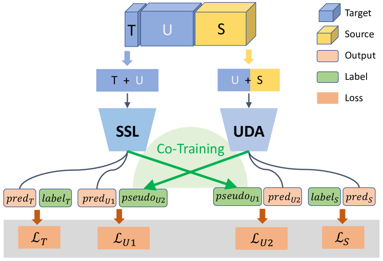
Figure 4: The overall framework of DeCoTa. It decomposes the SSDA task into SSL and UDA tasks that exchange pseudo-labels for unlabeled target U.

In section 5 of the main paper, we compare variants of our approach, including MiST, two-view MiST, and DeCoTa. Here we give some more discussions. These three methods are different by 1) how many classifiers they train; 2) what labeled data they use; 3) which classifier provides the pseudo-labels. Fig. 5 gives an illustrative comparison. Fig. 4 illustrates the framework pipeline of DeCoTa.

• MiST learns a single model $\bm{w}$, using both labeled source data $D_{\mathcal{S}}{}$ and labeled target data $D_{\mathcal{T}}{}$. MiST also updates $\bm{w}$ using pseudo-labels on the unlabeled target data $D_{\mathcal{U}}{}$, where the pseudo-labels are predicted by the current $\bm{w}$.

• Two-view MiST (i.e., two-task MiST) learns two models, $\bm{w}_{\color[rgb]{1,0,0}T}$ and $\bm{w}_{\color[rgb]{0,0,1}S}$ (cf. subsection 3.2 of the main paper). $\bm{w}_{\color[rgb]{1,0,0}T}$ is updated using $D_{\mathcal{T}}{}$ and pseudo-labeled data on $D_{\mathcal{U}}{}$, where the pseudo-labels are predicted by the current $\bm{w}_{\color[rgb]{1,0,0}T}$. $\bm{w}_{\color[rgb]{0,0,1}S}$ is updated using $D_{\mathcal{S}}{}$ and pseudo-labeled data on $D_{\mathcal{U}}{}$, where the pseudo-labels are predicted by the current $\bm{w}_{\color[rgb]{0,0,1}S}$.

• DeCoTa learns two models, $\bm{w}_{\color[rgb]{1,0,0}f}$ and $\bm{w}_{\color[rgb]{0,0,1}g}$. $\bm{w}_{\color[rgb]{1,0,0}f}$ is updated using $D_{\mathcal{T}}{}$ and pseudo-labeled data on $D_{\mathcal{U}}{}$, where the pseudo-labels are predicted by the current $\bm{w}_{\color[rgb]{0,0,1}g}$. $\bm{w}_{\color[rgb]{0,0,1}g}$ is updated using $D_{\mathcal{S}}{}$ and pseudo-labeled data on $D_{\mathcal{U}}{}$, where the pseudo-labels are predicted by the current $\bm{w}_{\color[rgb]{1,0,0}f}$.

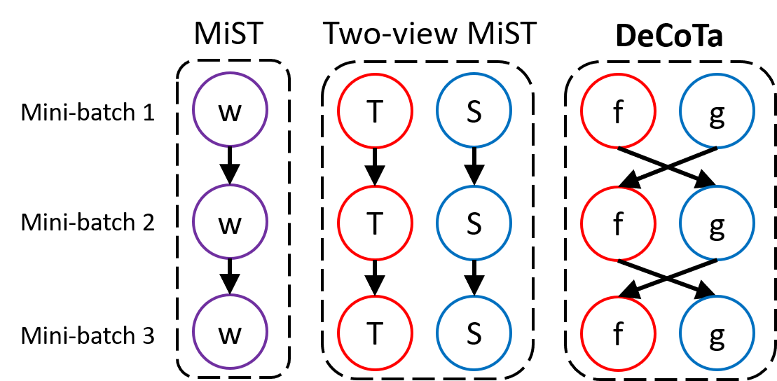
Figure 5: Comparison among MiST, two-view MiST (i.e., two-task MiST), and DeCoTa. The color on the circles means the labeled data: red for $D_{\mathcal{T}}{}$, blue for $D_{\mathcal{S}}{}$, and purple for both. The arrows indicate which model provides the pseudo-labels for which model to learn from.

DeCoTa has two hyper-parameters: the confidence threshold $\tau$ (cf. Equation 1 of the main paper) and $\alpha$ in MixUp (cf. Equation 2 of the main paper). We follow [51] to select these hyper-parameters using three other labeled examples per class in the target domain. Specifically, we only select hyper-parameters based on DomainNet three-shot setting, Real to Clipart. We then fix the selected hyper-parameters, $\tau=0.5$ and $\alpha=1.0$, for all other experiments.

Table 5: Accuracy on DomainNet (%) for the one-shot setting with four domains, using ResNet-34.

Method	R to C	R to P	P to C	C to S	S to P	R to S	P to R	Mean
S+T	58.1	61.8	57.7	51.5	55.4	49.1	73.1	58.1
DANN [13]	61.2	62.3	56.4	54.0	57.9	55.9	65.6	59.0
ENT [51]	60.0	60.2	54.9	48.3	55.8	49.4	74.4	57.6
MME [51]	69.5	68.1	64.4	56.7	62.0	59.2	76.9	65.3
UODA [45]	72.7	70.3	69.8	60.5	66.4	62.7	77.3	68.5
APE [26]	70.4	70.8	72.9	56.7	64.5	63.0	76.6	67.6
ELP [22]	72.8	70.8	72.0	59.6	66.7	63.3	77.8	69.0
DeCoTa	79.1	74.9	76.9	65.1	72.0	69.7	79.6	73.9

Table 6: Accuracy on Office-Home (%) for the one-shot setting with four domains, using VGG-16.

Method	R to C	R to P	R to A	P to R	P to C	P to A	A to P	A to C	A to R	C to R	C to A	C to P	Mean
S+T	39.5	75.3	61.2	71.6	37.0	52.0	63.6	37.5	69.5	64.5	51.4	65.9	57.4
DANN [13]	52.0	75.7	62.7	72.7	45.9	51.3	64.3	44.4	68.9	64.2	52.3	65.3	60.0
ENT [51]	23.7	77.5	64.0	74.6	21.3	44.6	66.0	22.4	70.6	62.1	25.1	67.7	51.6
MME [51]	49.1	78.7	65.1	74.4	46.2	56.0	68.6	45.8	72.2	68.0	57.5	71.3	62.7
UODA [45]	49.6	79.8	66.1	75.4	45.5	58.8	72.5	43.3	73.3	70.5	59.3	72.1	63.9
ELP [22]	49.2	79.7	65.5	75.3	46.7	56.3	69.0	46.1	72.4	68.2	67.4	71.6	63.1
DeCoTa	47.2	80.3	64.6	75.5	47.2	56.6	71.1	42.5	73.1	71.0	57.8	72.9	63.3

Table 7: Accuracy on Office-Home (%) for the three-shot setting with four domains, using ResNet-34.

Method	R to C	R to P	R to A	P to R	P to C	P to A	A to P	A to C	A to R	C to R	C to A	C to P	Mean
S+T	55.7	80.8	67.8	73.1	53.8	63.5	73.1	54.0	74.2	68.3	57.6	72.3	66.2
DANN [13]	57.3	75.5	65.2	69.2	51.8	56.6	68.3	54.7	73.8	67.1	55.1	67.5	63.5
ENT [51]	62.6	85.7	70.2	79.9	60.5	63.9	79.5	61.3	79.1	76.4	64.7	79.1	71.9
MME [51]	64.6	85.5	71.3	80.1	64.6	65.5	79.0	63.6	79.7	76.6	67.2	79.3	73.1
APE [26]	66.4	86.2	73.4	82.0	65.2	66.1	81.1	63.9	80.2	76.8	66.6	79.9	74.0
DeCoTa	70.4	87.7	74.0	82.1	68.0	69.9	81.8	64.0	80.5	79.0	68.0	83.2	75.7

Table 8: SSDA results on Office-31, on two scenarios (following [51]).

Method	Webcam (W) to Amazon (A)		DSLR (D) to Amazon (A)
	1-shot	3-shot	1-shot	3-shot
S+T	69.2	73.2	68.2	73.3
DANN [13]	69.3	75.4	70.4	74.6
ENT [51]	69.1	75.4	72.1	75.1
MME [51]	73.1	76.3	73.6	77.6
Ours	76.0	76.8	74.2	78.3

Appendix B Experimental Results

B.1 Main results on the one-shot setting

We report the comparison with baselines in the one-shot setting on DomainNet in Table 5 and Office-Home in Table 6. DeCoTa outperforms the state-of-the-art methods by $4.9\%$ on DomainNet (ResNet-34), while performs slightly worse than [45] by $0.6\%$ on Office-Home (VGG-16). Nevertheless, DeCoTa attains the highest accuracy on $5$ adaptation scenarios of Office-Home in the one-shot setting.

B.2 Office-Home results on other backbones

We report the comparison with baselines on Office-Home using a ResNet-34 backbone in Table 7, following [26]. DeCoTa attains the state-of-the-art result.

B.3 Results on Office-31

We report the comparison with available baseline results on Office-31 [50] in Table 8, using ResNet-34 backbone. Following [51], two adaptation scenarios are compared (Webcam to Amazon, DSLR to Amazon). Our approach DeCoTa consistently outperforms the compared methods.

B.4 Larger-shot results

We provide 10,20,50-shot SSDA results on DomainNet in Table 9. We randomly select and add additional samples per class from the target domain to the target labeled pool. As a semi-supervised setting, we compared with both domain adaptation (DA) and semi-supervised learning (SSL) baselines [59]. The implementation details are the same as those of 1,3-shot. DeCoTa improves along with more shots and can outperform baselines.

B.5 Numbers and accuracy of pseudo-labels

We showed the number of total and correct pseudo-labels by the two classifiers of DeCoTa along the training iterations in Figure 3 (c) of the main paper. The analysis is on DomainNet three-shot setting, from Real to Clipart. Concretely, for every $1K$ iterations (i.e., 24K unlabeled data), we accumulated the number of unlabeled data that have confident (with confidence $>\tau=0.5$) and correct predictions by at least one classifier. We further plot them independently for each classifier (i.e., $\bm{w}_{\color[rgb]{1,0,0}f}$ and $\bm{w}_{\color[rgb]{0,0,1}g}$) in Fig. 6. The accuracy of pseudo-labels remains stable (i.e., the number of confident and correct predictions divided by the number of confident predictions) but the number increases along training.

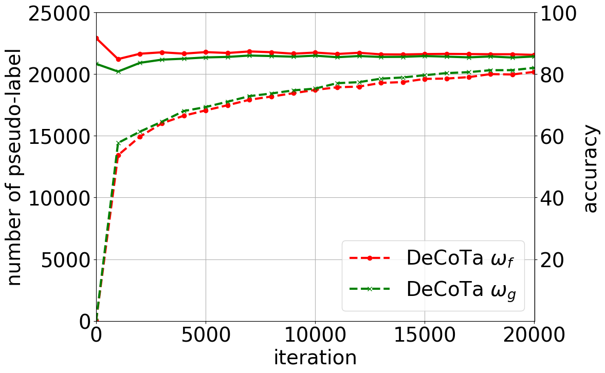
Figure 6: Number (dashed, left) and accuracy (solid, right) of pseudo-labels on DomainNet three-shot setting, Real to Clipart.

B.6 Task decomposition

We report the comparison of DeCoTa and MiST on DomainNet and Office-Home in all the adaptation scenarios. As shown in Table 10(b), DeCoTa outperform MiST on all the setting by $1\sim 2\%$ on DomainNet and $3\sim 5\%$ on Office-Home, which further confirms the effectiveness of task decomposition — explicitly considering the discrepancy between the two sources of supervision — in DeCoTa.

B.7 One-direction training

We further consider another variant of DeCoTa named one-direction teaching, in which only one task teaches the other. Instead of co-training, we use either $\bm{w}_{f}$ or $\bm{w}_{g}$ to generate pseudo-labels for both tasks, while keeping the other setups the same as DeCoTa. This study is designed to measure the complementary specialties of the two tasks. As shown in Table 11, the performance drops notably by using one-direction teaching. The results suggest that the two tasks provide unique expertise and complement each other, instead of one dominating the other.

B.8 Results on the source domain

We report the results on the source domain test set using $\bm{w}_{f}$ and $\bm{w}_{g}$ of DeCoTa on DomainNet (three-shot) in Table 12. While $\bm{w}_{f}$ and $\bm{w}_{g}$ have similar accuracy on the target domain test set, the fact that $\bm{w}_{f}$ does not learn from $D_{\mathcal{S}}{}$ suggests their difference in classifying source domain data. Table 12 confirms this: we see that $\bm{w}_{g}$ clearly dominates $\bm{w}_{f}$. Its accuracy is even on a par with a model trained only on $D_{\mathcal{S}}{}$, showing one advantage of DeCoTa— the model can keep its discriminative ability on the source domain.

B.9 Sensitivity to the confidence threshold $\tau$

We investigate DeCoTa’s sensitivity to the confidence threshold $\tau$ for assigning pseudo-labels (cf. Equation 1 and Equation 4 of the main paper). As shown in Fig. 7, the variance in accuracy is small when $\tau\leq 0.7$. The accuracy drops notably when $\tau\geq 0.9$. We surmise that it is due to too few pseudo-labeled data are picked under a high threshold.

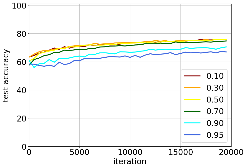
Figure 7: DeCoTa’s sensitivity to pseudo-label threshold $\tau$ on DomainNet three-shot setting, Real to Clipart.

B.10 Analysis on the Beta distribution coefficient $\alpha$

Fig. 8 shows DeCoTa’s sensitivity to the MixUp hyper-parameter $\alpha$ in Equation 2 of the main paper: $\alpha$ is the coefficient of the Beta distribution, which influences the sampled value of $\lambda$, an indicator of the “propotion” in the MixUp algorithm. We report DeCoTa’s result on DomainNet three-shot setting, adapting from Real to Clipart. The best performance is achieved by $\alpha=1.0$, equivalent to a uniform distribution of $\lambda\in[0,1]$. This result is consistent with our hypothesis that MixUp connects the source and target domains with interpolated feature spaces in-between.

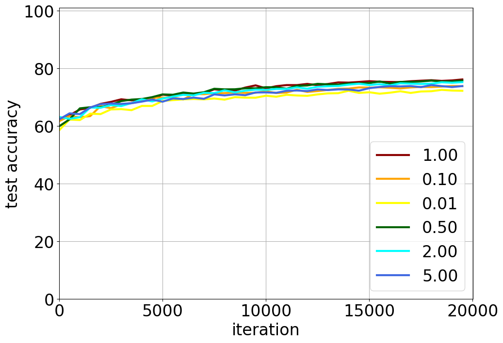
Figure 8: DeCoTa’s sensitivity to the Beta distribution coefficient $\alpha$ on DomainNet three-shot setting, Real to Clipart.

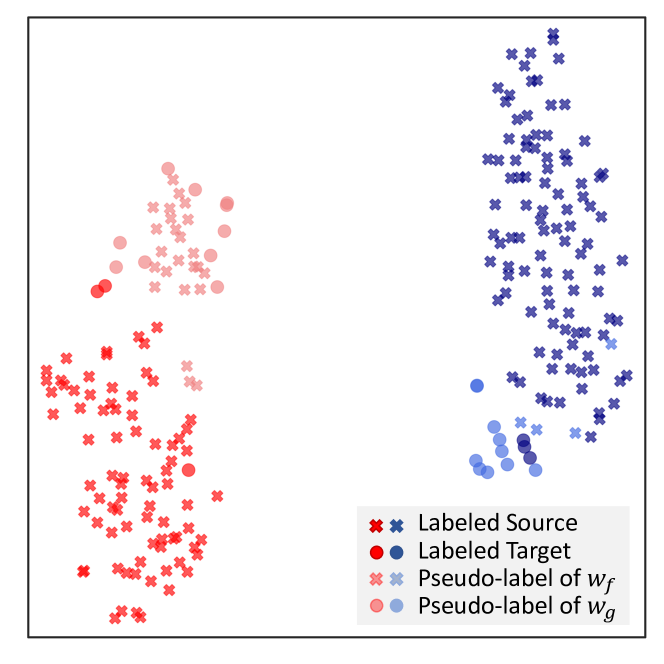
Figure 9: t-SNE visualization of pseudo-labels assigned by $\bm{w}_{f}$ and $\bm{w}_{g}$ in DeCoTa (see text for details).

B.11 Training time

DeCoTa does not increase the training time much for two reasons. First, at each iteration (i.e., mini-batch), it only updates and learns from the pseudo-labels of the current mini-batch of unlabeled data, not the entire unlabeled data. Second, assigning pseudo-labels only requires a forward pass of the mini-batch, just like most domain adaptation algorithms normally do to compute training losses. The only difference is that DeCoTa trains two classifiers and needs to perform the forward pass of unlabeled data twice.

B.12 t-SNE visualizations on DeCoTa tasks

We visualize $D_{\mathcal{S}}{}$, $D_{\mathcal{T}}{}$, and the $D_{\mathcal{U}}{}$ pseudo-labels by each task of DeCoTa in Fig. 9. For clarity, we select two classes for illustration. The colors blue and red represent the two classes; the shapes circle and cross represent data from $D_{\mathcal{T}}{}$ (labeled target data) and $D_{\mathcal{S}}{}$ (labeled source data), respectively. The colors light blue and light red represent the pseudo-labels of each class on $D_{\mathcal{U}}{}$, in which the shape circle indicates that the pseudo-labels are provided by $\bm{w}_{f}$ (learned with $D_{\mathcal{T}}{}$) and the shape cross indicates that the pseudo-labels are provided by $\bm{w}_{g}$ (learned with $D_{\mathcal{S}}{}$). The visualization is based on DomainNet three-shot setting, from Real to Clipart, trained for $10,000$ iterations. We see that $\bm{w}_{f}$ tends to assign pseudo-labels to unlabeled data whose features are closer to $D_{\mathcal{T}}{}$; $\bm{w}_{g}$ tends to assign pseudo-labels to unlabeled data whose features are closer to $D_{\mathcal{S}}{}$. Such a behavior is aligned with the seminal work of semi-supervised learning by [77].

Table 9: Results on DomainNet at 10, 20, 50-shot, using ResNet-34. We tune hyper-parameters for SSL methods similarly to DA methods.

	R to C			R to P			P to C			C to S			S to P			R to S			P to R			Mean
n-shot $\rightarrow$	10	20	50	10	20	50	10	20	50	10	20	50	10	20	50	10	20	50	10	20	50	10	20	50
S+T	69.1	72.4	77.5	67.3	70.2	73.4	68.2	72.5	77.7	62.9	67.3	71.8	64.8	67.9	72.6	61.3	65.5	70.2	78.0	79.3	82.2	67.4	70.7	75.1
DANN [13]	66.2	68.0	71.1	65.1	67.1	69.0	62.4	64.5	68.2	60.0	62.4	66.8	61.3	63.8	67.6	61.4	63.2	66.9	71.6	74.7	78.1	64.0	66.2	69.7
ENT [51]	77.9	80.0	83.0	72.3	74.9	77.7	77.5	79.1	82.3	66.3	70.1	75.0	66.3	71.0	75.7	63.9	68.3	74.6	81.2	82.9	84.5	72.2	75.2	79.0
MME [51]	77.0	78.5	80.9	71.9	74.0	76.4	75.6	76.9	80.4	65.9	68.6	72.5	68.6	70.9	74.4	66.7	69.7	72.7	80.8	82.2	83.3	72.4	74.4	77.2
Mixup [76]	73.4	79.5	83.1	68.3	72.2	75.4	75.0	79.5	83.1	63.7	69.4	75.0	68.5	72.4	76.2	62.9	69.9	75.0	78.8	82.3	84.7	70.1	75.0	78.9
FixMatch [59]	76.6	79.5	82.3	73.0	74.7	76.4	75.8	79.4	83.3	70.1	73.1	76.9	71.3	73.3	77.0	68.7	71.6	74.2	79.7	81.9	84.2	73.6	76.2	79.2
DeCoTa	81.8	82.6	85.0	75.1	76.6	78.7	81.3	81.7	84.5	73.7	75.3	78.0	73.4	75.7	77.7	73.7	75.5	77.8	80.7	80.1	83.9	77.1	78.2	80.8

Table 10: Comparison between DeCoTa and MiST: test accuracy on DomainNet and Office-Home dataset ($\%$).

(a) DomainNet

Setting	Method	R to C	R to P	P to C	C to S	S to P	R to S	P to R	Mean
1-shot	MiST	74.8	73.6	74.5	65.0	72.0	67.0	77.6	72.1
	DeCoTa	79.1	74.9	76.9	65.1	72.0	69.7	79.6	73.9
3-shot	MiST	78.1	75.2	76.7	68.3	72.6	71.5	79.8	74.6
	DeCoTa	80.4	75.2	78.7	68.6	72.7	71.9	81.5	75.6

(b) Office-Home

Setting	Method	R to C	R to P	R to A	P to R	P to C	P to A	A to P	A to C	A to R	C to R	C to A	C to P	Mean
1-shot	MiST	42.7	77.5	62.9	73.1	39.4	54.8	67.1	40.0	66.9	67.9	56.8	69.4	59.9
	DeCoTa	47.2	80.3	64.6	75.5	47.2	56.6	71.1	42.5	73.1	71.0	57.8	72.9	63.3
3-shot	MiST	54.7	81.2	64.0	69.4	51.7	58.8	69.1	47.6	70.6	65.3	60.8	73.8	63.9
	DeCoTa	59.9	83.9	67.7	77.3	57.7	60.7	78.0	54.9	76.0	74.3	63.2	78.4	69.3

Table 11: Comparison between DeCoTa and one-direction teaching: accuracy on DomainNet ($\%$) three-shot setting.

Method	R to C	R to P	P to C	C to S	S to P	R to S	P to R	Mean
$\bm{w}_{f}$ teaching	73.8	67.2	73.7	63.1	65.9	61.7	78.2	69.1
$\bm{w}_{g}$ teaching	77.5	74.5	74.2	64.8	71.6	69.0	79.0	72.9
DeCoTa	80.4	75.2	78.7	68.6	72.7	71.9	81.5	75.6

Table 12: Comparison on the source domain test data of DomainNet ($\%$). Here we compare the two-task models of DeCoTa in the three-shot setting to the source-only model (S).

Method	R to C	R to P	P to C	C to S	S to P	R to S	P to R	Mean
$\bm{w}_{f}$	55.2	68.2	43.8	59.5	50.8	56.9	61.0	56.3
$\bm{w}_{g}$	97.2	97.1	99.3	98.7	98.9	96.8	99.4	98.2
S	98.1	98.2	99.5	98.9	99.2	98.2	99.6	98.8

References

- [1] Shuang Ao, Xiang Li, and Charles X Ling. Fast generalized distillation for semi-supervised domain adaptation. In AAAI, 2017.
- [2] Maria-Florina Balcan, Avrim Blum, and Ke Yang. Co-training and expansion: Towards bridging theory and practice. In NIPS, 2005.
- [3] Michele Banko and Eric Brill. Scaling to very very large corpora for natural language disambiguation. In Proceedings of the 39th annual meeting on association for computational linguistics, pages 26–33. Association for Computational Linguistics, 2001.
- [4] Shai Ben-David, John Blitzer, Koby Crammer, Alex Kulesza, Fernando Pereira, and Jennifer Wortman Vaughan. A theory of learning from different domains. Machine learning, 79(1-2):151–175, 2010.
- [5] David Berthelot, Nicholas Carlini, Ian Goodfellow, Nicolas Papernot, Avital Oliver, and Colin A Raffel. Mixmatch: A holistic approach to semi-supervised learning. In NeurIPS, 2019.
- [6] Avrim Blum and Tom Mitchell. Combining labeled and unlabeled data with co-training. In COLT, 1998.
- [7] Minmin Chen, Kilian Q Weinberger, and John Blitzer. Co-training for domain adaptation. In NIPS, 2011.
- [8] Minmin Chen, Kilian Q Weinberger, and Yixin Chen. Automatic feature decomposition for single view co-training. In ICML, 2011.
- [9] Yuhua Chen, Wen Li, Christos Sakaridis, Dengxin Dai, and Luc Van Gool. Domain adaptive faster r-cnn for object detection in the wild. In CVPR, 2018.
- [10] Yi-Hsin Chen, Wei-Yu Chen, Yu-Ting Chen, Bo-Cheng Tsai, Yu-Chiang Frank Wang, and Min Sun. No more discrimination: Cross city adaptation of road scene segmenters. In Proceedings of the IEEE International Conference on Computer Vision, pages 1992–2001, 2017.
- [11] Jia Deng, Wei Dong, Richard Socher, Li-Jia Li, Kai Li, and Li Fei-Fei. Imagenet: A large-scale hierarchical image database. In CVPR, 2009.
- [12] Jeff Donahue, Judy Hoffman, Erik Rodner, Kate Saenko, and Trevor Darrell. Semi-supervised domain adaptation with instance constraints. In Proceedings of the IEEE conference on computer vision and pattern recognition, pages 668–675, 2013.
- [13] Yaroslav Ganin, Evgeniya Ustinova, Hana Ajakan, Pascal Germain, Hugo Larochelle, François Laviolette, Mario Marchand, and Victor Lempitsky. Domain-adversarial training of neural networks. JMLR, 17(1):2096–2030, 2016.
- [14] Boqing Gong, Kristen Grauman, and Fei Sha. Learning kernels for unsupervised domain adaptation with applications to visual object recognition. JMLR, 109(1-2):3–27, 2014.
- [15] Ian J Goodfellow, Jonathon Shlens, and Christian Szegedy. Explaining and harnessing adversarial examples. In ICLR, 2015.
- [16] Yves Grandvalet and Yoshua Bengio. Semi-supervised learning by entropy minimization. In NIPS, 2005.
- [17] Bo Han, Quanming Yao, Xingrui Yu, Gang Niu, Miao Xu, Weihua Hu, Ivor Tsang, and Masashi Sugiyama. Co-teaching: Robust training of deep neural networks with extremely noisy labels. In NeurIPS, 2018.
- [18] Kaiming He, Xiangyu Zhang, Shaoqing Ren, and Jian Sun. Deep residual learning for image recognition. In CVPR, 2016.
- [19] Geoffrey Hinton, Oriol Vinyals, and Jeff Dean. Distilling the knowledge in a neural network. arXiv preprint arXiv:1503.02531, 2015.
- [20] Judy Hoffman, Erik Rodner, Jeff Donahue, Trevor Darrell, and Kate Saenko. Efficient learning of domain-invariant image representations. In ICLR, 2013.
- [21] Judy Hoffman, Eric Tzeng, Taesung Park, Jun-Yan Zhu, Phillip Isola, Kate Saenko, Alexei A Efros, and Trevor Darrell. Cycada: Cycle-consistent adversarial domain adaptation. In ICML, 2018.
- [22] Zhiyong Huang, Kekai Sheng, Weiming Dong, Xing Mei, Chongyang Ma, Feiyue Huang, Dengwen Zhou, and Changsheng Xu. Effective label propagation for discriminative semi-supervised domain adaptation. arXiv preprint arXiv:2012.02621, 2020.
- [23] Naoto Inoue, Ryosuke Furuta, Toshihiko Yamasaki, and Kiyoharu Aizawa. Cross-domain weakly-supervised object detection through progressive domain adaptation. In CVPR, 2018.
- [24] Mehran Khodabandeh, Arash Vahdat, Mani Ranjbar, and William G Macready. A robust learning approach to domain adaptive object detection. In ICCV, 2019.
- [25] Seunghyeon Kim, Jaehoon Choi, Taekyung Kim, and Changick Kim. Self-training and adversarial background regularization for unsupervised domain adaptive one-stage object detection. In ICCV, 2019.
- [26] Taekyung Kim and Changick Kim. Attract, perturb, and explore: Learning a feature alignment network for semi-supervised domain adaptation. In ECCV, 2020.
- [27] Ananya Kumar, Tengyu Ma, and Percy Liang. Understanding self-training for gradual domain adaptation. In International Conference on Machine Learning, pages 5468–5479. PMLR, 2020.
- [28] Dong-Hyun Lee. Pseudo-label: The simple and efficient semi-supervised learning method for deep neural networks. In Workshop on challenges in representation learning, ICML, 2013.
- [29] Seungmin Lee, Dongwan Kim, Namil Kim, and Seong-Gyun Jeong. Drop to adapt: Learning discriminative features for unsupervised domain adaptation. In ICCV, 2019.
- [30] Da Li and Timothy Hospedales. Online meta-learning for multi-source and semi-supervised domain adaptation. arXiv preprint arXiv:2004.04398, 2020.
- [31] Limin Li and Zhenyue Zhang. Semi-supervised domain adaptation by covariance matching. TPAMI, 41(11):2724–2739, 2018.
- [32] Jian Liang, Ran He, Zhenan Sun, and Tieniu Tan. Distant supervised centroid shift: A simple and efficient approach to visual domain adaptation. In CVPR, 2019.
- [33] Mingsheng Long, Yue Cao, Jianmin Wang, and Michael I Jordan. Learning transferable features with deep adaptation networks. arXiv preprint arXiv:1502.02791, 2015.
- [34] Laurens van der Maaten and Geoffrey Hinton. Visualizing data using t-sne. Journal of machine learning research, 9(Nov):2579–2605, 2008.
- [35] Zhijun Mai, Guosheng Hu, Dexiong Chen, Fumin Shen, and Heng Tao Shen. Metamixup: Learning adaptive interpolation policy of mixup with meta-learning. arXiv preprint arXiv:1908.10059, 2019.
- [36] Xudong Mao, Yun Ma, Zhenguo Yang, Yangbin Chen, and Qing Li. Virtual mixup training for unsupervised domain adaptation. arXiv preprint arXiv:1905.04215, 2019.
- [37] David McClosky, Eugene Charniak, and Mark Johnson. Effective self-training for parsing. In ACL, 2006.
- [38] David McClosky, Eugene Charniak, and Mark Johnson. Reranking and self-training for parser adaptation. In ACL, 2006.
- [39] Adam Paszke, Sam Gross, Soumith Chintala, Gregory Chanan, Edward Yang, Zachary DeVito, Zeming Lin, Alban Desmaison, Luca Antiga, and Adam Lerer. Automatic differentiation in pytorch. 2017.
- [40] Zhongyi Pei, Zhangjie Cao, Mingsheng Long, and Jianmin Wang. Multi-adversarial domain adaptation. In Thirty-Second AAAI Conference on Artificial Intelligence, 2018.
- [41] Xingchao Peng, Qinxun Bai, Xide Xia, Zijun Huang, Kate Saenko, and Bo Wang. Moment matching for multi-source domain adaptation. In Proceedings of the IEEE International Conference on Computer Vision, pages 1406–1415, 2019.
- [42] Luis AM Pereira and Ricardo da Silva Torres. Semi-supervised transfer subspace for domain adaptation. Pattern Recognition, 75:235–249, 2018.
- [43] Viraj Prabhu, Arjun Chandrasekaran, Kate Saenko, and Judy Hoffman. Active domain adaptation via clustering uncertainty-weighted embeddings. arXiv preprint arXiv:2010.08666, 2020.
- [44] Siyuan Qiao, W. Shen, Zhishuai Zhang, Bo Wang, and A. Yuille. Deep co-training for semi-supervised image recognition. In ECCV, 2018.
- [45] Can Qin, Lichen Wang, Qianqian Ma, Yu Yin, Huan Wang, and Yun Fu. Opposite structure learning for semi-supervised domain adaptation. arXiv preprint arXiv:2002.02545, 2020.
- [46] Rajeev Ranjan, Carlos D Castillo, and Rama Chellappa. L2-constrained softmax loss for discriminative face verification. arXiv preprint arXiv:1703.09507, 2017.
- [47] Stephan R Richter, Vibhav Vineet, Stefan Roth, and Vladlen Koltun. Playing for data: Ground truth from computer games. In ECCV, 2016.
- [48] German Ros, Laura Sellart, Joanna Materzynska, David Vazquez, and Antonio M Lopez. The synthia dataset: A large collection of synthetic images for semantic segmentation of urban scenes. In CVPR, 2016.
- [49] Olga Russakovsky, Jia Deng, Hao Su, Jonathan Krause, Sanjeev Satheesh, Sean Ma, Zhiheng Huang, Andrej Karpathy, Aditya Khosla, Michael Bernstein, et al. Imagenet large scale visual recognition challenge. IJCV, 115(3):211–252, 2015.
- [50] Kate Saenko, Brian Kulis, Mario Fritz, and Trevor Darrell. Adapting visual category models to new domains. In ECCV, 2010.
- [51] Kuniaki Saito, Donghyun Kim, Stan Sclaroff, Trevor Darrell, and Kate Saenko. Semi-supervised domain adaptation via minimax entropy. In ICCV, 2019.
- [52] Kuniaki Saito, Yoshitaka Ushiku, Tatsuya Harada, and Kate Saenko. Adversarial dropout regularization. arXiv preprint arXiv:1711.01575, 2017.
- [53] Kuniaki Saito, Kohei Watanabe, Yoshitaka Ushiku, and Tatsuya Harada. Maximum classifier discrepancy for unsupervised domain adaptation. In CVPR, 2018.
- [54] Christos Sakaridis, Dengxin Dai, and Luc Van Gool. Semantic foggy scene understanding with synthetic data. International Journal of Computer Vision, 126(9):973–992, 2018.
- [55] Fatemeh Sadat Saleh, Mohammad Sadegh Aliakbarian, Mathieu Salzmann, Lars Petersson, and Jose M Alvarez. Effective use of synthetic data for urban scene semantic segmentation. In ECCV. Springer, 2018.
- [56] Swami Sankaranarayanan, Yogesh Balaji, Arpit Jain, Ser Nam Lim, and Rama Chellappa. Learning from synthetic data: Addressing domain shift for semantic segmentation. In CVPR, 2018.
- [57] Rui Shu, Hung H Bui, Hirokazu Narui, and Stefano Ermon. A dirt-t approach to unsupervised domain adaptation. In ICLR, 2018.
- [58] Karen Simonyan and Andrew Zisserman. Very deep convolutional networks for large-scale image recognition. arXiv preprint arXiv:1409.1556, 2014.
- [59] Kihyuk Sohn, David Berthelot, Chun-Liang Li, Zizhao Zhang, Nicholas Carlini, Ekin D Cubuk, Alex Kurakin, Han Zhang, and Colin Raffel. Fixmatch: Simplifying semi-supervised learning with consistency and confidence. In NeurIPS, 2020.
- [60] Jong-Chyi Su, Yi-Hsuan Tsai, Kihyuk Sohn, Buyu Liu, Subhransu Maji, and Manmohan Chandraker. Active adversarial domain adaptation. In WACV, 2020.
- [61] Yuhua Tang, Zhipeng Lin, Haotian Wang, and Liyang Xu. Adversarial mixup synthesis training for unsupervised domain adaptation. In ICASSP, 2020.
- [62] Qingyi Tao, Hao Yang, and Jianfei Cai. Zero-annotation object detection with web knowledge transfer. In ECCV, 2018.
- [63] Yi-Hsuan Tsai, Wei-Chih Hung, Samuel Schulter, Kihyuk Sohn, Ming-Hsuan Yang, and Manmohan Chandraker. Learning to adapt structured output space for semantic segmentation. In CVPR, 2018.
- [64] Eric Tzeng, Judy Hoffman, Trevor Darrell, and Kate Saenko. Simultaneous deep transfer across domains and tasks. In ICCV, 2015.
- [65] Eric Tzeng, Judy Hoffman, Ning Zhang, Kate Saenko, and Trevor Darrell. Deep domain confusion: Maximizing for domain invariance. arXiv preprint arXiv:1412.3474, 2014.
- [66] Hemanth Venkateswara, Jose Eusebio, Shayok Chakraborty, and Sethuraman Panchanathan. Deep hashing network for unsupervised domain adaptation. In CVPR, 2017.
- [67] Riccardo Volpi, Pietro Morerio, Silvio Savarese, and Vittorio Murino. Adversarial feature augmentation for unsupervised domain adaptation. In Proceedings of the IEEE Conference on Computer Vision and Pattern Recognition, pages 5495–5504, 2018.
- [68] Ximei Wang, Liang Li, Weirui Ye, Mingsheng Long, and Jianmin Wang. Transferable attention for domain adaptation. In Proceedings of the AAAI Conference on Artificial Intelligence, volume 33, pages 5345–5352, 2019.
- [69] Yan Wang, Chen Xiangyu, You Yurong, Erran Li Li, Bharath Hariharan, Mark Campbell, Kilian Q. Weinberger, and Chao Wei-Lun. Train in germany, test in the usa: Making 3d object detectors generalize. In CVPR, 2020.
- [70] Colin Wei, Kendrick Shen, Yining Chen, and Tengyu Ma. Theoretical analysis of self-training with deep networks on unlabeled data. arXiv preprint arXiv:2010.03622, 2020.
- [71] Minghao Xu, Jian Zhang, Bingbing Ni, Teng Li, Chengjie Wang, Qi Tian, and Wenjun Zhang. Adversarial domain adaptation with domain mixup. In AAAI, 2020.
- [72] Shen Yan, Huan Song, Nanxiang Li, Lincan Zou, and Liu Ren. Improve unsupervised domain adaptation with mixup training. arXiv preprint arXiv:2001.00677, 2020.
- [73] Luyu Yang, Yogesh Balaji, Ser-Nam Lim, and Abhinav Shrivastava. Curriculum manager for source selection in multi-source domain adaptation. arXiv preprint arXiv:2007.01261, 2020.
- [74] Ting Yao, Yingwei Pan, Chong-Wah Ngo, Houqiang Li, and Tao Mei. Semi-supervised domain adaptation with subspace learning for visual recognition. In CVPR, 2015.
- [75] Xingrui Yu, Bo Han, Jiangchao Yao, Gang Niu, Ivor Tsang, and Masashi Sugiyama. How does disagreement help generalization against label corruption? In International Conference on Machine Learning, pages 7164–7173. PMLR, 2019.
- [76] Hongyi Zhang, Moustapha Cisse, Yann N Dauphin, and David Lopez-Paz. mixup: Beyond empirical risk minimization. In ICLR, 2018.
- [77] Xiaojin Jerry Zhu. Semi-supervised learning literature survey. Technical report, University of Wisconsin-Madison Department of Computer Sciences, 2005.
- [78] Yang Zou, Zhiding Yu, BVK Vijaya Kumar, and Jinsong Wang. Unsupervised domain adaptation for semantic segmentation via class-balanced self-training. In ECCV, 2018.