CKM Substructure

Abstract

The CKM matrix is not generic. The Wolfenstein parametrization encodes structure by having one small parameter, $\lambda\approx 0.22$. We pose the question: is there substructure in the CKM matrix that goes beyond the single small parameter of the Wolfenstein parameterization? We find two relations that are approximately satisfied: $|V_{td}|^{2}=|V_{cb}|^{3}$ and $|V_{ub}|^{2}|V_{us}|=|V_{cb}|^{4}$. We discuss the statistical significance of these relations and find that they may indicate deeper structure in the CKM matrix. The current precision, however, cannot exclude an $\mathcal{O}(10\%)$ accident.

I Introduction

The CKM matrix is not generic. This fact is captured by the Wolfenstein parameterization Wolfenstein:1983yz

$$V=\pmatrix{1-\frac{1}{2}\lambda^{2}&\lambda&A\lambda^{3}(\rho-i\eta)\cr-\lambda&1-\frac{1}{2}\lambda^{2}&A\lambda^{2}\cr A\lambda^{3}(1-\rho-i\eta)&-A\lambda^{2}&1\cr}+\mathcal{O}(\lambda^{4})\;.$$ (1)

The assumption in writing the above approximation is that $\lambda\approx 0.22$ is the only small parameter, while $A$, $\eta$, and $\rho$ are all $\mathcal{O}(1)$.

In this paper we ask the following question: is there hidden structure in the CKM matrix? In other words, are there relations among CKM elements beyond the hierarchies captured by the Wolfenstein parametrization?

A similar question has been asked regarding mixing in the lepton sector where a clear hierarchy is not present and the PMNS matrix is not close to the unit matrix. Is there structure in the PMNS matrix? While we do not know the answer, two avenues have been explored. On the one hand there are indications for structure, for example tri-bimaximal mixing Harrison:2002er , and many models have been proposed to explain it, notably based on $A_{4}$ (for a review see, for example, Ref. King:2015aea ). An alternative framework is known as anarchy Hall:1999sn ; Haba:2000be ; deGouvea:2003xe ; deGouvea:2012ac ; Lu:2014cla . The PMNS matrix is defined to be anarchic by the authors of Ref. Hall:1999sn when “all entries are comparable, no pattern or structure is easily discernable, and there are no special precise ratios between any entries.”

The question we would like to pose can be framed in a similar way to the question that was asked about the lepton sector. To do this we define the term Wolfenstein anarchy. A CKM matrix is Wolfenstein anarchic if, besides the one small parameter $\lambda$, the matrix is otherwise generic. There should be no special precise relations among parameters except those predicted by the Wolfenstein parameterization. Is the CKM matrix found in Nature Wolfenstein anarchic?

The hierarchical nature of the CKM matrix motivates UV completions that dynamically generate the small parameter $\lambda$. For example, Froggatt–Nielson (FN) models Froggatt:1978nt ; Leurer:1992wg ; Leurer:1993gy ; Ibanez:1994ig dynamically generate the parameter $\lambda$ as a ratio of mass scales, and the special form of the CKM matrix is a consequence of symmetries where fermions from different generations have different charges. These models predict hierarchies but only up to $\mathcal{O}(1)$ numbers, which depend on $\mathcal{O}(1)$ parameters within the UV completion. Therefore, FN models predict that the CKM matrix respects Wolfenstein anarchy.

In exploring whether the CKM matrix is consistent with Wolfenstein anarchy we found two relations that hold to a good approximation beyond the ones that are direct results of the Wolfenstein hierarchy. They are

$$|V_{td}|^{2}=|V_{cb}|^{3},\qquad|V_{ub}|^{2}={|V_{cb}|^{4}\over|V_{us}|}\,,$$ (2)

When combined, these relations lead to

$$\left|{V_{td}\over V_{ub}}\right|^{2}=\left|{V_{us}\over V_{cb}}\right|\,.$$ (3)

In term of the Wolfenstein parameters these relations are given by

$$A=\eta^{2}+(1-\rho)^{2},\qquad A^{2}\lambda=\eta^{2}+\rho^{2}\,.$$ (4)

When combined we can write them as

$${\eta^{2}+\rho^{2}\over\eta^{2}+(1-\rho)^{2}}=A\lambda\,,$$ (5)

or as an $A$-independent relation

$$\left[\eta^{2}+(1-\rho)^{2}\right]^{2}\lambda=\eta^{2}+\rho^{2}.$$ (6)

There are two questions that we would like to ask about these relations:

1. What UV flavor models can generate them?

2. Are they an indication of CKM substructure or are they consistent with Wolfenstein anarchy?

Regarding the first question, we tried to find a UV model that generates these relations, but were so far unable to do so. The second question, on the other hand, is what we discuss below.

II Fits of the CKM matrix elements

We search for relations of the form

$$\prod_{n}|V_{{i_{n}}{j_{n}}}|^{a_{n}}\prod_{m}|V_{{k_{m}}{l_{m}}}|^{-b_{m}}=1\,,$$ (7)

where $i_{n}$ and $k_{m}$ are selected from $(u,c,t)$, $j_{n}$ and $l_{m}$ are selected from $(d,s,b)$, $V$ with any two subindices represents an element of the CKM matrix, and $a_{n}$ and $b_{n}$ are positive integers. We use the following criteria when looking for relations

1. We check for relations that involve a small number of CKM elements, which we choose to be six, that is

   $$\sum_{n}a_{n}+\sum_{m}b_{m}\leq 6\,.$$ (8)

2. We look for relations such that their central values are very close to one, concretely, those that fall within $2\%$ of one.

3. We do not consider relations that are a result of the Wolfenstein parameterization, for example, $|V_{us}|=|V_{cd}|$ is not a new relation.

Based on these criteria, and the central values of the CKM elements from CKMfitter Charles:2004jd , we found exactly two independent relations, which are given by Eq. (2).

We next assess the statistical significance of these relations. The CKMfitter code, modified to check for relations, is used to find Sebastien

$$R_{1}\equiv\left|{V_{td}^{2}\over V_{cb}^{3}}\right|=1.004^{+0.026}_{-0.023}\,,\qquad R_{2}\equiv\left|{V_{ub}^{2}V_{us}\over V_{cb}^{4}}\right|=0.994^{+0.066}_{-0.044}\,.$$ (9)

The input values and statistical procedure of this fit can be found in Ref. Charles:2004jd . Fig. 1. shows the same result as a correlated plot.

A few remarks are in order:

1. The central values of both relations are within $1\%$ of 1.

2. The errors in $R_{2}$ are larger basically since the error on $\left|V_{ub}\right|$ is the largest among the CKM elements (see for example the “CKM Quark-Mixing Matrix” review in Ref. PDG2020 ).

3. The errors are asymmetric, which indicates that there are significant correlations in deriving the errors and the errors are not just simply statistical.

4. There is no strong correlation in the statistical errors between the two relations.

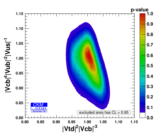
Figure 1: The correlation between the two relations, $R_{1}$ and $R_{2}$, defined in Eq. (9) Sebastien .

III A test for Wolfenstein Anarchy

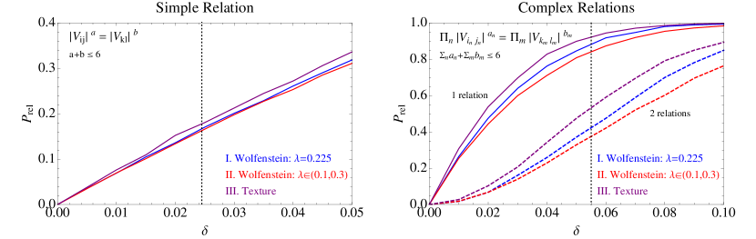
Figure 2: Left: The probability of finding at least one simple relation, as defined in Eq. (12), as a function of the precision, $\delta$. Random CKM matrices are generated using Wolfenstein Anarchy with fixed $\lambda$ (blue), Wolfenstein anarchy with random $\lambda$ (red), and random Yukawa matrices using textures with random coefficients (purple). Parameters are randomly generated as described in Eqs. (10), (11), and (15). Right: The probability of finding at least one (solid) or at least two (dashed) complex relations, as defined in Eq. (13). The colors correspond to different scans, as on the left. The vertical black lines at $\delta=0.0245$ and $\delta=0.055$, on the left and right, respectively, correspond to the (symmetrized) precision of the $R_{1,2}$ fits, see Eq. (9).

Figure 3: The black dots show the $(\eta,\rho)$ (left) and $(A,\rho)$ (right) of $10^{4}$ CKM matrices generated with Wolfenstein Anarchy that satisfy at least 1 simple relation, Eq. (12) with precision $\delta=0.02$. For this scan we fix $\lambda=0.225$. We find that 13% of random CKM matrices satisfy at least one relation. The blue dots correspond to random CKM matrices that satisfy relation $R_{1}$, $A=\eta^{2}+(1-\rho)^{2}$. The red dot is the observed CKM matrix. Several structures that are clearly visible in the plot correspond to relations that appear in Table 1, such as $A=1$ and $\rho=1/2$.

		probability (%)
		scan I	scan II	scan III
Wolfenstein	CKM	$\lambda=0.225$	$\lambda\in(0.1,0.3)$	texture
$A=1$	$V_{cb}=V_{us}^{2}$	3.7	3.7	0.8
$A\sqrt{(1-\rho)^{2}+\eta^{2}}=1$	$V_{td}=V_{us}^{3}$	2.6	2.6	0.7
$A\sqrt{\rho^{2}+\eta^{2}}=1$	$V_{ub}=V_{us}^{3}$	1.9	1.9	0.6
$A=(1-\rho)^{2}+\eta^{2}$	$V_{td}^{2}=V_{cb}^{3}$	1.4	1.4	0.7
$A=\rho^{2}+\eta^{2}$	$V_{ub}^{2}=V_{cb}^{3}$	1.0	1.0	0.6
$\rho=1/2$	$V_{ub}=V_{td}$	0.9	0.9	2.3
$A\sqrt{\rho^{2}+\eta^{2}}=\lambda$	$V_{ub}=V_{us}^{4}$	0.8	0.7	0.6
$A\lambda=\sqrt{\rho^{2}+\eta^{2}}$	$V_{ub}=V_{cb}^{2}$	0.7	0.5	0.5
$A\sqrt{(1-\rho)^{2}+\eta^{2}}=\lambda$	$V_{td}=V_{us}^{4}$	0.2	0.1	0.5
$A\lambda=\sqrt{(1-\rho)^{2}+\eta^{2}}$	$V_{td}=V_{cb}^{2}$	0.1	0.1	0.4
other		0.02	0.03	6.0

Table 1: We generated $10^{6}$ random CKM matrices using the prescriptions of scans I, II, and III, described by Eqs. (10), (11), and (15). We find that 13%, 13%, and 14%, respectively, satisfy at least one simple relation, as in Eq. (12), with precision $\delta=0.02$. We show the 10 most common relations for scan I. The first column shows each relation as a function of Wolfenstein parameters, and the second column is an example of how the relation manifests as a function of CKM matrix elements. The final three columns show the probability that a random CKM matrix, from each scan, satisfies the relation with precision $\delta=0.02$. The last row shows the probability of satisfying additional relations not listed in this table.

Are the relations of Eq. (9) evidence of CKM substructure, or are they consistent with Wolfenstein anarchy? This question can be addressed using a statistical model for Wolfenstein anarchy. Given an ensemble of randomly generated CKM matrices that are consistent with the Wolfenstein parameterization, is it exceedingly unlikely to satisfy the relations of Eq. (9)? There is a “trials factor” because there are many possible relations that could, in principle, be satisfied. In order to assess the likelihood that the observed relations are random occurrences, we have used a computer to randomly generate many CKM matrices and checked the probability that they satisfy the above, or similar, relations.

We generate ensembles of random CKM matrices using two methods, described below. First, we generate random Wolfenstein parameters directly. Second, we generate random Yukawa matrices using textures, motivated by FN models, with random coefficients. For alternate approaches to generating random CKM matrices see Refs. Froggatt:1979sz ; Rosenfeld:2001sc .

III.1 Random CKM Matrices from Wolfenstein Anarchy

We generate ensembles of CKM matrices by choosing random Wolfenstein parameters according to two prescriptions, which we label as scan I and scan II. For these scans we generate random Wolfenstein parameters with uniform (linear) probability distributions in the following ranges,

$$({\rm\mathbf{I}}) \quad\lambda=0.225\,, \quad A\in(0.5-1.5)\,,\quad\sqrt{\rho^{2}+\eta^{2}}\in(0.2-1)\,,\quad\theta\in(0,2\pi)$$ (10)

$$({\rm\mathbf{II}}) \quad\lambda\in(0.1-0.3)\,, \quad A\in(0.5-1.5)\,,\quad\sqrt{\rho^{2}+\eta^{2}}\in(0.2-1)\,,\quad\theta\in(0,2\pi)\,\,,$$ (11)

where we write $\rho+i\eta=\sqrt{\rho^{2}+\eta^{2}}\,e^{i\theta}$ and separately generate the magnitude and phase. Scan I fixes $\lambda$ to the observed value, while scan II allows $\lambda$ to vary between 0.1 and 0.3.

We first look for CKM matrices satisfying a simple relation of the form:

$$\left||V_{ij}|^{a}|V_{jk}|^{-b}-1\right|<\delta\qquad\qquad a+b\leq 6\,,$$ (12)

where $\delta$ is the precision by which the relation is satisfied. This is a generalization of $R_{1}$ of Eq. (9). The left of Fig. 2 shows the probability that at least one simple relation is satisfied as a function of the precision, $\delta$. For this test and the tests described below, we generate $10^{6}$ random matrices, and we use all of them or a subset, making sure that that the statistical uncertainty is far smaller than the uncertainties in Eq. (9). The vertical dashed line corresponds to $\delta=0.0245$, which is the current precision fitting to $R_{1}$ after symmetrizing the uncertainties, see Eq. (9). We find a probability of 16% (15%) that a random CKM matrix satisfies at least one relation to this precision for scan I (II).

To further study the probability to have relations, we check the probability that a random matrix satisfies one or more relations with precision $\delta=0.02$. We find a probability of $13\%$ for this to be the case for both scans. Fig. 3 shows the locations of these points in the $(\rho,\eta)$ and $(A,\rho)$ planes as black dots. (To generate the plot we use a subset of $10^{4}$ of the matrices that satisfy one or more relations.) We find that 1.4% of random CKM matrices satisfy $R_{1}$, corresponding to the relation $A=\eta^{2}+(1+\rho)^{2}$. These points are denoted by blue dots. The red dot corresponds to the observed values of the Wolfenstein parameters.

While there is a percent-level chance that a random CKM matrix satisfies $R_{1}$ to the observed precision, there is evidently an order-of-magnitude larger probability that a similar relation is satisfied. What other relations are being satisfied, for example, by the black dots in Fig. 3? Using the generated random CKM matrices, the 10 most common relations are collected in Table 1. The table lists the probability that each relation is satisfied with a precision of $\delta=0.02$ for scans I and II. We observe similar probabilities for both scans. Several of the relations are clearly visible as clusters of points in Fig. 3, such as $A=1$ and $\rho=1/2$. Relations not shown in the table together account for less than 0.02% (0.03%) of random matrices for scan I (II).

We next look for more complicated relations of the form,

$$\left|\prod_{n}|V_{{i_{n}}{j_{n}}}|^{a_{n}}\prod_{m}|V_{{k_{m}}{l_{m}}}|^{-b_{m}}-1\right|<\delta\qquad\qquad\sum_{n}a_{n}+\sum_{m}b_{m}\leq 6\,,$$ (13)

generalizing $R_{2}$ from above. These relations include the simple relations of Eq. (12). The right side of Fig. 2 shows the probability of satisfying 1 or 2 of these relations. There is a large probability of satisfying one relation of this form because of the large number of possible relations. For example the probability of satisfying one complex relation to a precision of $\delta=0.02$ is 48% (44%) for $\lambda$ fixed (varied). The probability that a randomly generated matrix satisfies two relations with $\delta=0.02$ simultaneously is only 7%. The vertical dashed line shows $\delta=.055$, which is the current precision for fitting $R_{2}$. We find that the probability of satisfying 2 relations with this precision is about 40%.

III.2 Random CKM Matrices from Textures

The purpose of Wolfenstein anarchy is to capture the types of CKM matrices that we expect to be generated by UV completions that generate the hierarchical structure of the CKM matrix, such as Froggatt-Nielson Froggatt:1978nt ; Leurer:1992wg ; Leurer:1993gy ; Ibanez:1994ig . We would like to verify: does generating random Wolfenstein parameters produce similar results to generating random Yukawa matrices?

In order to answer this question we have also used a computer to generate random Yukawa matrices. We assume the following textures Leurer:1993gy ,

$$Y_{d}=\left(\begin{array}[]{ccc}c_{11}\lambda^{6}&c_{12}\lambda^{5}&c_{13}\lambda^{5}\\ c_{21}\lambda^{5}&c_{22}\lambda^{4}&c_{23}\lambda^{4}\\ c_{31}\lambda^{3}&c_{32}\lambda^{2}&c_{33}\lambda^{2}\end{array}\right)\qquad Y_{u}=\left(\begin{array}[]{ccc}d_{11}\lambda^{6}&d_{12}\lambda^{4}&d_{13}\lambda^{3}\\ d_{21}\lambda^{5}&d_{22}\lambda^{3}&d_{23}\lambda^{2}\\ d_{31}\lambda^{3}&d_{32}\lambda&d_{33}\end{array}\right)$$ (14)

where $\lambda=0.225$ and $c_{ij}$ and $d_{ij}$ are random $\mathcal{O}(1)$ constants. For alternate textures that could also be considered, see for example Ref. Ibanez:1994ig .

Scan III is defined by selecting the following parameters with uniform (linear) probability distributions,

$$({\rm\mathbf{III}}) \qquad\lambda=0.225 \qquad|c_{ij}|,|d_{ij}|\in(0.2-5)\qquad\arg(c_{ij}),\arg(d_{ij})\in(0,2\pi)\,\,.$$ (15)

Note that a specific UV completion may predict correlations among the various coefficients, but for simplicity we do not include any correlations here.

Fig. 2 shows the probability of satisfying simple and complex relations from random textures, compared to the Wolfenstein anarchy approach described above. We find similar probabilities in both cases, confirming that the simpler Wolfenstein anarchy approach captures the behavior of random Yukawa matrices built from hierarchical textures.

We also generate $10^{6}$ random Yukawa matrices using the prescription of scan III, and look for simple relations of the form of Eq. (12) with a precision $\delta=0.02$. We find that 14% of random matrices in scan III satisfy one or more relation with this precision. This is similar to the 13% rate, found above, for scans I and II. Table 1 shows the probability of satisfying various relations for all three scans. Interestingly, although the overall rate of satisfying one or more relations is similar across all three scans, scan III exhibits a different pattern of relative probabilities for satisfying the various relations.

IV Discussion and conclusions

The main result of our paper is Eq. (9) where we point out two relations between CKM parameters. We are interested in them because they may point towards a deeper structure that generates the flavor parameters of the SM. Using the current values of the CKM parameters, the relations hold to a precision on the order of a few percent. This observation led us to define the notion of “Wolfenstein anarchy” where the assumption is that there is one small parameter, $\lambda$, and there is no additional structure in the quark flavor sector. We then perform a simple statistical analysis to find out what is the probability that such relations are a result of Wolfenstein anarchy. We find that with current uncertainties on the values of the parameters, and accounting for the trials factor of satisfying other similar relations, the probability is not $\mathcal{O}(1)$, but is also not small, that is, the probability is above $10\%$.

In order to make progress testing our relations, we require advances in both the theoretical and experimental inputs for the extraction of CKM parameters. In a few years, we expect that CKM fits will achieve the precision to either show that our relations are violated, or to confirm that they hold with a precision to disfavor the ansatz of Wolfenstein anarchy. At present, we think that it is too early to make this call, and therefore our purpose in this paper is simply to point out these relations and to suggest a simple framework for assessing their significance.

Note that the CKM elements run Balzereit:1998id ; JuarezWysozka:2002kx . To a good approximation only $A$ runs. The above two papers do not agree on the exact magnitude of the effect. In the SM, they found that the value of $A$ is reduced by $13\%$ Balzereit:1998id ($25\%$ JuarezWysozka:2002kx ) from the weak scale to the GUT scale. The running can be different in cases that there are new fields, beyond the SM, with masses below the scale where the flavor physics is generated. If the relations we studied here do come from some fundamental UV physics, what is important are the values of the CKM elements at the scale where this UV physics is generated. Assuming the SM and given the current $2\sigma$ errors on the values of the parameters, this implies that the relations $R_{1}$ and $R_{2}$ can be satisfied at a scale that is roughly below $10^{6}$ ($10^{5}$) GeV using Ref. Balzereit:1998id (Ref. JuarezWysozka:2002kx ). The relation we found in Eq. (6) is independent of $A$ and thus is to a very good approximation independent of the scale where the flavor structure is generated.

Assuming that the relations we found do come from a UV theory, this imposes a model-building challenge. In fact, we were unable to construct a model to explain either of the relations. The main challenge is that most UV models of flavor have more parameters in the UV than in the IR. In our case, however, we encounter the opposite situation: our IR relations suggest that the UV theory should have fewer parameters.

Finally, we remark that there could in principle be more relations beyond the types that we search for. In particular, we only look for relations of the form $a-b=0$, where $a$ and $b$ are the products of a few magnitudes of CKM elements. One can envision relations with more than two terms, with other proportionality factors between terms, or with dependence on the phase.

While the current precision does not allow us to claim that the relations of Eq. (9) hint at a deep fact about UV physics, they motivate searching for UV models that can explain them.

References

- (1) L. Wolfenstein, Phys. Rev. Lett. 51, 1945 (1983).
- (2) P. F. Harrison, D. H. Perkins and W. G. Scott, Phys. Lett. B 530, 167 (2002) [hep-ph/0202074].
- (3) S. F. King, J. Phys. G 42, 123001 (2015) [arXiv:1510.02091 [hep-ph]].
- (4) L. J. Hall, H. Murayama and N. Weiner, Phys. Rev. Lett. 84, 2572 (2000) [hep-ph/9911341].
- (5) N. Haba and H. Murayama, Phys. Rev. D 63, 053010 (2001) [hep-ph/0009174].
- (6) A. de Gouvea and H. Murayama, Phys. Lett. B 573, 94 (2003) [hep-ph/0301050].
- (7) A. de Gouvea and H. Murayama, Phys. Lett. B 747, 479 (2015) [arXiv:1204.1249 [hep-ph]].
- (8) X. Lu and H. Murayama, JHEP 1408, 101 (2014) [arXiv:1405.0547 [hep-ph]].
- (9) C. D. Froggatt and H. B. Nielsen, Nucl. Phys. B 147, 277 (1979).
- (10) M. Leurer, Y. Nir and N. Seiberg, Nucl. Phys. B 398, 319 (1993) [hep-ph/9212278].
- (11) M. Leurer, Y. Nir and N. Seiberg, Nucl. Phys. B 420, 468 (1994) [hep-ph/9310320].
- (12) L. E. Ibanez and G. G. Ross, Phys. Lett. B 332, 100 (1994) [hep-ph/9403338].
- (13) J. Charles et al. [CKMfitter Group], Eur. Phys. J. C 41, no.1, 1-131 (2005) [arXiv:hep-ph/0406184 [hep-ph]]. Updated results and plots available at: http://ckmfitter.in2p3.fr
- (14) Sébastien Descotes-Geno, private communication.
- (15) P.A. Zyla et al. (Particle Data Group), to be published in Prog. Theor. Exp. Phys. 2020, 083C01 (2020).
- (16) C. D. Froggatt and H. B. Nielsen, Nucl. Phys. B 164, 114 (1980).
- (17) R. Rosenfeld and J. L. Rosner, Phys. Lett. B 516, 408 (2001) [hep-ph/0106335].
- (18) C. Balzereit, T. Mannel and B. Plumper, Eur. Phys. J. C 9, 197 (1999) [hep-ph/9810350].
- (19) S. R. Juarez Wysozka, S. F. Herrera H., P. Kielanowski and G. Mora, Phys. Rev. D 66, 116007 (2002) [hep-ph/0206243].