and : efficient conformal regions in high dimensions

Abstract

Conformal methods create prediction bands that control average coverage assuming solely i.i.d. data. Although the literature has mostly focused on prediction intervals, more general regions can often better represent uncertainty. For instance, a bimodal target is better represented by the union of two intervals. Such prediction regions are obtained by CD-split, which combines the split method and a data-driven partition of the feature space which scales to high dimensions. CD-split however contains many tuning parameters, and their role is not clear. In this paper, we provide new insights on CD-split by exploring its theoretical properties. In particular, we show that CD-split converges asymptotically to the oracle highest predictive density set and satisfies local and asymptotic conditional validity. We also present simulations that show how to tune CD-split. Finally, we introduce HPD-split, a variation of CD-split that requires less tuning, and show that it shares the same theoretical guarantees as CD-split. In a wide variety of our simulations, CD-split and HPD-split have better conditional coverage and yield smaller prediction regions than other methods.

1 Goals in Conformal Prediction

Most supervised machine learning methods yield a point estimate for a target, $Y\in{\mathcal{Y}}$, based on features, ${\mathbf{X}}\in{\mathcal{X}}$. However, it is often more informative to present prediction bands, that is, a subset of ${\mathcal{Y}}$ with plausible values for $Y$ (Neter et al.,, 1996). A particular way of constructing prediction bands is through conformal predictions (Vovk et al.,, 2005, 2009). Conformal predictions generate a predictive region for a future target, $Y_{n+1}$, based on features, ${\mathbf{X}}_{n+1}$, and past observations $({\mathbf{X}}_{1},Y_{1}),\ldots,({\mathbf{X}}_{n},Y_{n})$. An appealing property of the conformal methodology is that it controls the marginal coverage of prediction bands assuming solely exchangeable data (Kallenberg,, 2006):

Definition 1.

A conformal prediction, ${C_{\alpha}}({\mathbf{X}}_{n+1})$, satisfies marginal validity if

$${\mathbb{P}}\left(Y_{n+1}\in C({\mathbf{X}}_{n+1})\right) \geq 1-\alpha, \text{where }1-\alpha\text{is a coverage level.}$$

Besides marginal validity one might also wish for stronger guarantees. For instance, one might desire adequate coverage for each new instance and not solely on average across instances. This property is named conditional validity:

Definition 2.

A conformal prediction satisfies conditional validity if,

$${\mathbb{P}}(Y_{n+1}\in{C_{\alpha}}(\textbf{X}_{n+1})|\textbf{X}_{n+1}=\textbf{x}_{n+1}) \geq 1-\alpha, \text{for every }\ {\mathbf{x}}_{n+1}\in{\mathcal{X}}.$$

Unfortunately, conditional validity can be obtained only under strong assumptions about the distribution of $({\mathbf{X}},Y)$ (Vovk,, 2012; Lei and Wasserman,, 2014; Barber et al.,, 2019). Given this result, effort has been focused on obtaining intermediate conditions, such as local validity:

Definition 3.

A conformal prediction satisfies local validity if,

$${\mathbb{P}}(Y_{n+1}\in{C_{\alpha}}(\textbf{X}_{n+1})|\textbf{X}_{n+1}\in A) \geq 1-\alpha, \text{ for every }A\text{ in a partition of }\ {\mathcal{X}}.$$

Current methods that obtain local validity compute conformal regions using only training instances that fall in $A$ (Lei and Wasserman,, 2014; Barber et al.,, 2019; Guan,, 2019). However, these methods do not scale to high-dimensional settings because it is challenging to create $A$ that is large enough so that many training instances fall in $A$, and yet small enough so that local validity is close to conditional validity.

Another alternative is to obtain conditional validity at the specified level as the sample size increases (Lei et al.,, 2018):

Definition 4.

A conformal prediction satisfies asymptotic conditional validity if, there exist random sets, $\Lambda_{n}$, such that ${\mathbb{P}}({\mathbf{X}}_{n+1}\in\Lambda_{n}|\Lambda_{n})=1-o_{{\mathbb{P}}}(1)$ and

$$\sup_{{\mathbf{x}}_{n+1}\in\Lambda_{n}}\big{|}{\mathbb{P}}(Y_{n+1}\in C(\textbf{X}_{n+1})|\textbf{X}_{n+1}={\mathbf{x}}_{n+1})-(1-\alpha)\big{|}=o(1).$$

In a regression context in which ${\mathcal{Y}}=\mathbb{R}$, Lei et al., (2018) obtains asymptotic conditional coverage under assumptions such as $Y=\mu({\mathbf{X}})+\epsilon$, where $\epsilon$ is independent of ${\mathbf{X}}$ and has density symmetric around 0. Also, asymptotic conditional coverage was obtained under weaker conditions with methods based on quantile regression (Sesia and Candès,, 2019; Romano et al.,, 2019) and cumulative distribution function (cdf) estimators (Chernozhukov et al.,, 2019; Izbicki et al.,, 2020).

Besides validity, it is also desirable to obtain small prediction regions. For instance, some of the methods in the last paragraph converge to the interval with the smallest length among the ones with adequate conditional coverage. However, even the oracle interval can be large. For instance, Figure 1 presents a case in which, for large values of ${\mathbf{X}}$, $Y$ is bimodal. In this case, the interval-based conformal method in the left provides large prediction bands, since it must include the low density region between the modes of the distribution.

Multimodal data such as in Figure 1 often occurs in applications (Hyndman et al.,, 1996; De Gooijer and Zerom,, 2003; Dutordoir et al.,, 2018). For instance, theory predicts that the density of the redshift of a galaxy based on its photometric features is highly asymmetrical and often multimodal (Schmidt et al.,, 2020). Taking these multimodalities into account is necessary to obtain reliable cosmological inferences (Wittman,, 2009), as further discussed in Section 6.

Whenever relevant multimodalities exist, a conformal method should be able to yield regions which are not intervals. Moreover, ideally it should converge to the highest predictive density set (hpd), which can be considerably smaller than the smallest interval:

Definition 5 (Convergence to the highest predictive density set).

The highest predictive density set, ${C_{\alpha}^{*}}({\mathbf{x}})$, is the region with the smallest Lebesgue measure with the specified $1-\alpha$ coverage:

$${C_{\alpha}^{*}}({\mathbf{x}}) :=\left\{y:f(y|{\mathbf{x}})>{q_{\alpha}}({\mathbf{x}})\right\}, {q_{\alpha}}({\mathbf{x}}) \alpha f(Y|{\mathbf{X}}) {\mathbf{X}}={\mathbf{x}}$$ where is the quantile of given that .

A conformal prediction method converges to the highest predictive density set if:

$${\mathbb{P}}(Y_{n+1}\in{C_{\alpha}^{*}}({\mathbf{X}}_{n+1})\triangle{C_{\alpha}}({\mathbf{X}}_{n+1})) =o(1), A\triangle B:=(A\cap B^{c})\cup(B\cap A^{c})$$ where

Conformal methods that converge to the highest predictive density set satisfy asymptotic conditional coverage, as proved in section A.1:

Theorem 6.

If a conformal method converges to the highest predictive density set, then it satisfies asymptotic conditional coverage.

To the best of our knowledge, CD-split (Izbicki et al.,, 2020), is the only conformal method that has the goal of approximating the highest predictive density sets in high-dimensional feature spaces. As a result, CD-split attains prediction regions that are considerably smaller than the ones obtained from interval-based methods, as illustrated in Figure 1. However, Izbicki et al., (2020) shows only empirically that CD-split converges to the highest predictive density sets.

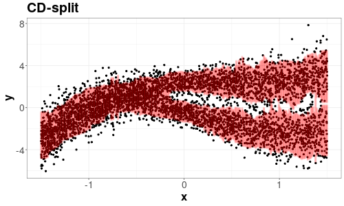
Figure 1: Comparison between a conformal method based on intervals (left) and CD-split when $Y|{\mathbf{X}}$ is bimodal.

In this paper, we further investigate conformal methods that converge to the oracle highest predictive density set. With respect to CD-split, we prove that it satisfies local and asymptotic conditional validities, and also converges to the oracle highest density set. We also perform many simulation studies which guide the choice in CD-split’s tuning parameters. Next, we introduce a new method, HPD-split, which requires less tuning parameters than CD-split, while having similar theoretical guarantees and similar performance in simulations. In order to obtain such properties, HPD-split uses an informative conformity score which, under weak assumptions, is approximately independent of the features.

Section 2 reviews some conformal prediction strategies that appear in the literature. Section 3 describes the proposed conformal conditional density estimation methods. Section 4 presents the main theoretical properties of the proposed methods. In particular, it is shown that all proposed methods satisfy marginal and asymptotic conditional validity and converge to the highest predictive density set. Section 5 uses several new experiments based on simulations to show how to tune CD-split and to compare CD-split and HPD-split to other existing methods. Section 6 demonstrates the performance of CD-split and HPD-split in an application of photometric redshift prediction. All proofs are in the Appendix.

2 Review of some conformal prediction strategies

The main goal in conformal predictions is to use the data to obtain a valid prediction region, $C({\mathbf{X}}_{n+1})$. A general strategy for obtaining such a region is the split method (Papadopoulos et al.,, 2002; Vovk,, 2012; Lei et al.,, 2018). Under this method, the data is divided into two sets: the training set, ${\mathbb{D}}^{\prime}=\{({\mathbf{X}}^{\prime}_{1},Y^{\prime}_{1}),\ldots,({\mathbf{X}}^{\prime}_{n},Y^{\prime}_{n})\}$, and the prediction set, ${\mathbb{D}}=\{({\mathbf{X}}_{1},Y_{1}),\ldots,({\mathbf{X}}_{m},Y_{m})\}$. We define $m=n$ solely to simplify notation. Next, a conformity score, ${\widehat{g}}:{\mathcal{X}}\times{\mathcal{Y}}\rightarrow{\mathbb{R}}$, is trained using ${\mathbb{D}}^{\prime}$. Finally, ${\mathbb{D}}$ is used for calculating $U_{i}:={\widehat{g}}({\mathbf{X}}_{i},Y_{i})$, the split residuals. Since the split residuals are assumed to be exchangeable, the rank of $U_{n+1}$ is uniform among $\{1,\ldots,n+1\}$ and, by letting $U_{\lfloor\alpha\rfloor}$ to be the $\lfloor n\alpha\rfloor$ order statistic among $U_{1},\ldots,U_{n}$, obtain that

$${\mathbb{P}}\left(U_{n+1}\geq U_{\lfloor\alpha\rfloor}\right) \geq 1-\alpha$$

$${\mathbb{P}}\left({\widehat{g}}({\mathbf{X}}_{n+1},Y_{n+1})\geq U_{\lfloor\alpha\rfloor}\right) \geq 1-\alpha$$

$${\mathbb{P}}\left(Y_{n+1}\in\left\{y:{\widehat{g}}({\mathbf{X}}_{n+1},y)\geq U_{\lfloor\alpha\rfloor}\right\}\right) \geq 1-\alpha.$$

That is, $C({\mathbf{X}}_{n+1})=\left\{y:{\widehat{g}}({\mathbf{X}}_{n+1},y)\geq U_{\lfloor\alpha\rfloor}\right\}$ is a marginally valid prediction region. However, in order to obtain stronger types of validity, it might be necessary to change the definition of the cutoff, $U_{\lfloor\alpha\rfloor}$, so that it adapts to the value of ${\mathbf{X}}_{n+1}$.

One way to obtain this adaptivity is to calculate the cutoff using solely the instances in ${\mathbb{D}}$ with covariates close to ${\mathbf{X}}_{n+1}$. For instance, Lei and Wasserman, (2014) divides ${\mathcal{X}}$ in a partition, ${\mathcal{A}}$, and compute $U_{\lfloor\alpha\rfloor}$ using solely the instances that fall in the same partition element as ${\mathbf{X}}_{n+1}$, as in Definition 7.

Definition 7.

Let ${\mathcal{A}}$ be a partition of ${\mathcal{X}}$. For each $A\in{\mathcal{A}}$, let

$$A({\mathbf{X}}_{n+1})=\{({\mathbf{X}},Y)\in{\mathbb{D}}:\exists A\in{\mathcal{A}}\text{ s.t. }{\mathbf{X}}\in A\text{ and }{\mathbf{X}}_{n+1}\in A\}$$

Let $U_{i}={\widehat{g}}({\mathbf{X}}_{i},Y_{i})$ be computed for each $({\mathbf{X}}_{i},Y_{i})$ in $A({\mathbf{X}}_{n+1})$. $U_{\lfloor\alpha\rfloor}({\mathbf{X}}_{n+1})$ is the $\lfloor|A({\mathbf{X}}_{n+1})|\cdot\alpha\rfloor$ order statistic of these $U_{i}$.

Since the split residuals in Definition 7 are exchangeable, one still obtains marginal validity by substituting $U_{\lfloor\alpha\rfloor}$ for $U_{\lfloor\alpha\rfloor}({\mathbf{X}}_{n+1})$ in the split method.

Theorem 8.

If ${\mathbb{D}}=\{({\mathbf{X}}_{1},Y_{1}),\ldots,({\mathbf{X}}_{n},Y_{n}),({\mathbf{X}}_{n+1},Y_{n+1})\}$ are exchangeable, then

$$C({\mathbf{X}}_{n+1})=\left\{y:{\widehat{g}}({\mathbf{X}}_{n+1},y)\geq U_{\lfloor\alpha\rfloor}({\mathbf{X}}_{n+1})\right\}$$

satisfies marginal validity and local validity with respect to $\mathcal{A}$.

The methods introduced in this paper are based on the above strategies, as described in the following section.

3 Conformal predictions based on conditional density estimators

Our proposed methods are based on conditional density estimators. In all of them, the conformity score, $\hat{g}$, is a function of an estimator of the conditional density of $Y$ given ${\mathbf{X}}$, $f(y|{\mathbf{x}})$. This conditional density estimator is denoted by ${\widehat{f}}(y|{\mathbf{x}})$. Since ${\widehat{f}}(y|{\mathbf{x}})$ is defined no matter whether $Y$ is discrete or continuous, the proposed methods are applicable both to conformal regression and to conformal classification. When ${\mathcal{Y}}$ is discrete, ${\widehat{f}}$ is a conditional probability estimate, $\hat{P}(y|{\mathbf{x}})$.

All of the proposed methods use the random variable $Z:=f(Y|{\mathbf{X}})$. The conditional cumulative density function (cdf) of $f(Y|{\mathbf{X}})$, $H(z|{\mathbf{x}})$, and its estimate, ${\hat{H}}(z|{\mathbf{x}})$, are presented in Definition 9:

Definition 9.

$H(z|{\mathbf{x}})$ and ${\hat{H}}(z|{\mathbf{x}})$ are, respectively, the conditional cdf of $f(Y|{\mathbf{X}})$ and its estimate:

$$H(z|{\mathbf{x}}) :=\int_{\{y:f(y|{\mathbf{x}})\leq z\}}{f(y|{\mathbf{x}})dy}$$

$${\hat{H}}(z|{\mathbf{x}}) :=\int_{\{y:{\widehat{f}}(y|{\mathbf{x}})\leq z\}}{{\widehat{f}}(y|{\mathbf{x}})dy}$$

Note that $H(z|{\mathbf{x}})$ is the conditional cdf of $f(Y|{\mathbf{X}})$, which is different from $F(y|{\mathbf{x}})$, the conditional cdf of $Y$. Besides these quantities, the conditional quantiles of $f(Y|{\mathbf{X}})$, ${q_{\alpha}}({\mathbf{x}})$, and their estimates, ${\hat{q}_{\alpha}}({\mathbf{x}})$, are also useful:

Definition 10.

${q_{\alpha}}({\mathbf{x}}):=H^{-1}(\alpha|{\mathbf{x}})$ is the $\alpha$-quantile of $f(Y|{\mathbf{X}})$. Also, ${\hat{q}_{\alpha}}({\mathbf{x}}):={\hat{H}}^{-1}(\alpha|{\mathbf{x}})$ is an estimate of the conditional $\alpha$-quantile of $f(Y|{\mathbf{X}})$.

Given the above definitions, it is possible to describe the proposed methods.

3.1 CD-split

CD-split uses the split method and adaptive cutoffs. In CD-split, the conformity score, ${\widehat{g}}$, is a conditional density estimator, ${\widehat{f}}(y|{\mathbf{x}})$:

Definition 11.

The CD-split residual is $U_{i}:={\widehat{f}}(Y_{i}|{\mathbf{X}}_{i})$.

CD-split also uses the partition method, as outlined in Definition 7. The performance of this method is highly dependent on the chosen partition. For instance, if the partition were defined according to the Euclidean distance on the feature space, then CD-split would not scale to high-dimensional feature spaces (Lei and Wasserman,, 2014; Barber et al.,, 2019; Tibshirani et al.,, 2019). In these settings small Euclidean neighborhoods have few data points and, therefore, the partition would be composed of large neighborhoods. As a result, each partition element would contain features with drastically varying densities, that is, the method would deviate strongly from conditional coverage. CD-split avoids this problem by choosing a partition such that, if ${\mathbf{x}}_{i}$ and ${\mathbf{x}}_{j}$ fall in the same partition element, then $U_{i}={\widehat{f}}(Y_{i}|{\mathbf{x}}_{i})$ and $U_{j}={\widehat{f}}(Y_{j}|{\mathbf{x}}_{j})$ have similar $\alpha$ quantiles. Definition 12 formalizes this idea:

Definition 12 (CD-split partition).

Let $\mathcal{I}$ be a partition of $\mathbb{R}^{+}$. ${\mathcal{A}}$ is a partition of ${\mathcal{X}}$ such that ${\mathbf{x}}_{i}$ and ${\mathbf{x}}_{j}$ are in the same partition element of ${\mathcal{A}}$ if and only if $\hat{q}_{\alpha}({\mathbf{x}}_{i})$ and $\hat{q}_{\alpha}({\mathbf{x}}_{j})$ are in the same partition element of $\mathcal{I}$.

Definition 12 partitions the feature space in a way that is directly related to conditional coverage. As a result, coarse partitions can still deviate weakly from conditional coverage.

By combining the ideas above, it is possible to formally define CD-split.

Definition 13 (CD-split).

Let $U_{\lfloor\alpha\rfloor}({\mathbf{X}}_{n+1})$ (Definition 7) be computed using the partition in Definition 12. The CD-split conformal prediction, $C({\mathbf{X}}_{n+1})$ is:

$$C({\mathbf{x}}_{n+1})=\left\{y:{\widehat{f}}(y|{\mathbf{x}}_{n+1})\geq U_{\lfloor\alpha\rfloor}({\mathbf{X}}_{n+1})\right\},$$ (1)

Algorithm 1 summarizes the implementation of CD-split.

Algorithm 1 CD-split

Input: Data $({\mathbf{x}}_{i},y_{i})$, $i=1,...,n$, coverage level $1-\alpha\in(0,1)$, algorithm $\mathcal{B}$ for fitting conditional density function, a partition of $\mathbb{R}^{+}$, $\mathcal{I}$.
Output: Prediction band for ${\mathbf{x}}_{n+1}\in\mathbb{R}^{d}$

1:  Randomly split $\{1,2,...,n\}$ into two subsets ${\mathbb{D}}$ and ${\mathbb{D}}^{\prime}$

2:  Compute $\hat{f}=\mathcal{B}(\{({\mathbf{x}}_{i},y_{i}):i\in{\mathbb{D}}^{\prime}\})$  // Estimate conditional density

3:  Use $\hat{f}$ to compute ${\hat{q}_{\alpha}}({\mathbf{x}}_{i})$, a quantile estimate, for each $({\mathbf{x}}_{i},y_{i})\in{\mathbb{D}}$  // (Definition 10)

4:  Determine $A({\mathbf{x}}_{n+1})$, the set of $({\mathbf{x}}_{i},y_{i})\in{\mathbb{D}}^{\prime}$ such that ${\hat{q}_{\alpha}}({\mathbf{x}}_{i})$ and ${\hat{q}_{\alpha}}({\mathbf{x}}_{n+1})$ belong to the same partition element of $\mathcal{I}$  // (Definitions 7 and 12)

5:  Compute $U_{\lfloor\alpha\rfloor}({\mathbf{x}}_{n+1})$, the $\alpha$-quantile of $\left\{{\widehat{f}}(y_{i}|{\mathbf{x}}_{i}):({\mathbf{x}}_{i},y_{i})\in A({\mathbf{x}}_{n+1})\right\}$

6:  Build a finite grid over $\mathcal{Y}$ and, by interpolation, return $\left\{y:{\widehat{f}}(y|{\mathbf{x}}_{n+1})\geq U_{\lfloor\alpha\rfloor}({\mathbf{x}}_{n+1})\right\}$

By observing eq. 1, it is possible to obtain some intuition on the theoretical properties of CD-split. If ${\widehat{f}}\approx f$ and ${\mathcal{A}}$ is a sufficiently fine partition, then for every ${\mathbf{x}}\in A({\mathbf{x}}_{n+1})$, ${q_{\alpha}}({\mathbf{x}})\approx{q_{\alpha}}({\mathbf{x}}_{n+1})$. As a result, if there are many instances in $A({\mathbf{x}}_{n+1})$ $U_{\lfloor\alpha\rfloor}({\mathbf{x}}_{n+1})\approx{q_{\alpha}}({\mathbf{x}}_{n+1})$ and $C({\mathbf{x}}_{n+1})\approx\{y:f(y|{\mathbf{x}}_{n+1})\geq{q_{\alpha}}({\mathbf{x}}_{n+1})\}$, the oracle conformal prediction. If the conditional density is well estimated, then the conformal band is close to the oracle band, as discussed in section 4.2.

Despite the above desirable properties, the partition in CD-split requires many tuning parameters. The following subsection introduces HPD-split, which avoids the partition method while yielding conformal regions similar to the ones in CD-split.

3.2 HPD-split

Several of the tuning parameters in CD-split follow from the fact that its conformity score is not approximately independent of the features, ${\mathbf{X}}$. Indeed, observe that CD-split uses $\hat{f}(Y|{\mathbf{X}})$ as a conformity score. Since the conditional distribution of $f(Y|{\mathbf{X}})$ is generally not independent of ${\mathbf{X}}$, the conformity score in CD-split is not approximately independent of ${\mathbf{X}}$. As a result, in order to obtain properties such as asymptotic conditional coverage, CD-split relies on the partition-method in section 2, which increases the number of tuning parameters. Given the above considerations, one might imagine that it is possible to reduce the number of tuning parameters in CD-split by choosing a conformity score that is approximately independent of ${\mathbf{X}}$.

The idea above is the main intuition for HPD-split. In HPD-split, the conformity score is ${\hat{H}}({\widehat{f}}(y|{\mathbf{x}})|{\mathbf{x}})$ instead of ${\widehat{f}}(y|{\mathbf{x}})$ (recall Definition 9). Observe that $H(z|{\mathbf{x}})$ is the conditional cdf of $f(Y|{\mathbf{X}})$ and, therefore, $H(f(Y|{\mathbf{X}})|{\mathbf{X}})\sim U(0,1)$ given ${\mathbf{X}}$. That is, $H(f(Y|{\mathbf{X}})|{\mathbf{X}})$ is independent of ${\mathbf{X}}$. Therefore, if ${\widehat{f}}(y|{\mathbf{x}})$ converges to $f(y|{\mathbf{x}})$, then one might expect that the conformity score ${\hat{H}}({\widehat{f}}(Y|{\mathbf{X}}))$ is approximately independent of ${\mathbf{X}}$. As a result, the partition method need not be used. The HPD-split residuals are formalized in Definition 14:

Definition 14 (HPD-split residual).

The HPD-split residuals are given by

$$U_{i} :={\hat{H}}\left({\widehat{f}}(Y_{i}|{\mathbf{X}}_{i})|{\mathbf{X}}_{i}\right)=\int_{\left\{y:{\widehat{f}}(y|{\mathbf{X}}_{i})\leq\hat{f}(Y_{i}|{\mathbf{X}}_{i})\right\}}{{\widehat{f}}(y|{\mathbf{X}}_{i})dy}.$$

The HPD-split residual is the area of the curve ${\widehat{f}}$ below ${\widehat{f}}(Y_{i}|{\mathbf{X}}_{i})$ (the shaded area in fig. 2). HPD-split uses this residual in the standard split method:

Definition 15 (HPD-split).

The HPD-split conformal prediction is

$$C({\mathbf{x}}_{n+1}):= \left\{y:{\hat{H}}\left({\widehat{f}}(y|{\mathbf{x}}_{n+1})|{\mathbf{x}}_{n+1}\right)\geq U_{\lfloor\alpha\rfloor}\right\}$$

$$= \left\{y:{\widehat{f}}(y|{\mathbf{x}}_{n+1})\geq{\hat{H}}^{-1}\left(U^{\text{hpd}}_{\lfloor\alpha\rfloor}\ |{\mathbf{x}}_{n+1}\right)\right\}.$$ (2)

Algorithm 2 summarizes the implementation of HPD-split.

Figure 2: The HPD-split score of sample $({\mathbf{x}}_{i},y_{i})$ is given by the shaded area on the plot.

By observing Definition 15, it is possible to obtain some intuition on the theoretical properties of HPD-split. If ${\widehat{f}}\approx f$, then $U_{i}\approx U(0,1)$ and $U^{\text{hpd}}_{\lfloor\alpha\rfloor}\approx\alpha$. Similarly, since ${\widehat{f}}\approx f$, ${\hat{H}}^{-1}\approx H^{-1}$ and ${\hat{H}}^{-1}(\alpha|{\mathbf{x}})\approx{q_{\alpha}}({\mathbf{x}})$. By combining these approximations in Definition 15, one obtains that $C({\mathbf{x}}_{n+1})\approx\left\{y:f(y|{\mathbf{x}}_{n+1})\geq{q_{\alpha}}({\mathbf{x}}_{n+1})\right\}$, the oracle highest predictive set. Indeed, HPD-split converges to the highest predictive set and satisfies asymptotic conditional validity, as discussed in section 4.2.

If $Y$ is discrete, then HPD-split is equivalent to the adaptive method proposed by Romano et al., (2020). The CQC method (Cauchois et al.,, 2021) is an alternative when $Y$ is discrete that also satisfies asymptotic conditional validity.

Algorithm 2 HPD-split

Input: Data $({\mathbf{x}}_{i},Y_{i})$, $i=1,...,n$, coverage level $1-\alpha\in(0,1)$, algorithm $\mathcal{B}$ for fitting conditional density function.
Output: Prediction band for ${\mathbf{x}}_{n+1}\in\mathbb{R}^{d}$

1:  Randomly split $\{1,2,...,n\}$ into two subsets ${\mathbb{D}}$ and ${\mathbb{D}}^{\prime}$

2:  Fit $\hat{f}=\mathcal{B}(\{({\mathbf{x}}_{i},Y_{i}):i\in{\mathbb{D}}^{\prime}\})$  // Estimate conditional density function

3:  Let $\hat{H}$ be an estimate of the cdf of the split residuals, $\hat{f}(Y|{\mathbf{X}})$, obtained by numerical integration (Definition 9).  // Estimate of split residual cdf

4:  Let $U_{\lfloor\alpha\rfloor}$ be the $\alpha$-quantile of $\left\{{\hat{H}}\left({\widehat{f}}(y_{i}|{\mathbf{x}}_{i})|{\mathbf{x}}_{i}\right):i\in\mathbb{D}\right\}$.

5:  Build a finite grid over $\mathcal{Y}$ and, by interpolation, return $\left\{y:{\hat{H}}\left({\widehat{f}}(y|{\mathbf{x}}_{n+1})|{\mathbf{x}}_{n+1}\right)\geq U_{\lfloor\alpha\rfloor}\right\}$.

Despite the simplicity of HPD-split, the partition method can obtain better conditional coverage in a few scenarios. The following section presents an improved partition, which is used to define CD-split⁺.

3.3 CD-split⁺: improved partitions

CD-split partitions the feature space based on solely the estimated conditional $\alpha$ quantiles of the CD-split residuals. Given this partition’s reliance on a single point, CD-split might be unstable in some scenarios. An alternative in Izbicki et al., (2020) is to build a partition based on the full estimate of the cdf of the CD-split residuals, ${\hat{H}}(z|{\mathbf{x}})$:

Definition 16 (Profile distance).

The profile distance between ${\mathbf{x}}_{a},{\mathbf{x}}_{b}\in\mathcal{X}$ is

$$d^{2}({\mathbf{x}}_{a},{\mathbf{x}}_{b}) :=\int_{-\infty}^{\infty}\left({\hat{H}}(z|{\mathbf{x}}_{a})-{\hat{H}}(z|{\mathbf{x}}_{b})\right)^{2}dz,$$

The profile distance is chosen so that two goals are satisfied. First, if two instances are close, then their split residuals have approximately the same conditional distribution. As a result, if one chooses a partition in such a way that all instances are close in the profile distance, then the instances are approximately exchangeable conditionally on ${\mathbf{X}}_{n+1}$. Second, two points can be close in the profile distance even though they are far apart in the Euclidean distance. As a result, the profile distance avoids the curse of dimensionality and has a large number of instances even in partitions composed of small neighborhoods. This idea is illustrated in Examples 17 and 18:

Example 17.

[Location family] Let ${\widehat{f}}(y|{\mathbf{x}})=h(y-\mu({\mathbf{x}}))$, where $h(y)$ is a density and $\mu({\mathbf{x}})$ an arbitrary function. In this case, $d({\mathbf{x}}_{a},{\mathbf{x}}_{b})=0$, for every ${\mathbf{x}}_{a},{\mathbf{x}}_{b}\in\mathbb{R}^{d}$. For instance, if $Y|{\mathbf{X}}\sim N(\beta^{t}{\mathbf{X}},\sigma^{2})$, then all split residuals have the same conditional distribution. A partition based on the profile distance would have a single element.

Example 18.

[Irrelevant features] If  ${\mathbf{x}}_{S}$ is a subset of the features such that ${\widehat{f}}(y|{\mathbf{x}})={\widehat{f}}(y|{\mathbf{x}}_{S})$, then $d({\mathbf{x}}_{a},{\mathbf{x}}_{b})$ does not depend on the irrelevant features, $S^{c}$. While irrelevant features do not affect the profile distance, have a large impact in the Euclidean distance in high-dimensional settings.

The profile distance is also related to CD-split. Note that $d({\mathbf{x}}_{a},{\mathbf{x}}_{b})=0$ if and only if the split residuals ${\widehat{f}}(Y|{\mathbf{x}}_{a})$ and ${\widehat{f}}(Y|{\mathbf{x}}_{b})$ have the same estimated conditional cdfs. That is, ${\hat{q}_{\alpha}}({\mathbf{x}}_{a})={\hat{q}_{\alpha}}({\mathbf{x}}_{b})$, for every $\alpha$. In this sense, while CD-split generates a partition that compares ${\hat{q}_{\alpha}}({\mathbf{x}}_{a})$ and ${\hat{q}_{\alpha}}({\mathbf{x}}_{b})$ for a single $\alpha$, the profile distance can be used to create a partition that compares these values for every $\alpha\in[0,1]$, as formalized in Theorem 19:

Theorem 19 (Theorem 3.9 in Izbicki et al., (2020)).

Let ${\widehat{f}}(\cdot|{\mathbf{x}})$ be a density w.r.t. the Lebesgue measure, for every ${\mathbf{x}}\in{\mathcal{X}}$. The equivalence relation ${\mathbf{x}}_{a}\sim{\mathbf{x}}_{b}\iff d({\mathbf{x}}_{a},{\mathbf{x}}_{b})=0$ is the minimal equivalence relation s.t., if ${\hat{q}_{\alpha}}({\mathbf{x}}_{a})={\hat{q}_{\alpha}}({\mathbf{x}}_{b})$ for every $\alpha\in[0,1]$, then ${\mathbf{x}}_{a}\sim{\mathbf{x}}_{b}$.

The profile distance induces a new partition over ${\mathcal{X}}$, which is used to define CD-split⁺:

Definition 20 (CD-split⁺).

Let ${\mathbf{C}}_{1}^{{}^{\prime}},\ldots,{\mathbf{C}}_{J}^{{}^{\prime}}$ be centroids for ${\mathbf{X}}_{1}^{{}^{\prime}},\ldots,{\mathbf{X}}_{n}^{{}^{\prime}}$ from ${\mathbb{D}}^{{}^{\prime}}$ according to $d$, the profile distance (Definition 16). Let ${\mathcal{A}}$ be a partition of ${\mathcal{X}}$ such that ${\mathbf{x}}\in A_{j}$ if and only if $d^{2}({\mathbf{x}},{\mathbf{C}}_{j}^{{}^{\prime}})<d^{2}({\mathbf{x}},{\mathbf{C}}_{k}^{{}^{\prime}})$, for every $k\neq j$. That is, ${\mathcal{A}}$ is the Voronoi partition generated from ${\mathbf{C}}_{1}^{{}^{\prime}},\ldots,{\mathbf{C}}_{J}^{{}^{\prime}}$ and $d^{2}$. CD-split⁺is defined in the same way as CD-split (Definition 13), but using this Voronoi partition instead of the one in Definition 12.

In practice, several algorithms might be used for determining the centroids in Definition 20. Here, for each $i\in{\mathbb{D}}$, we let ${\mathbf{w}}_{i}$ be a discretization obtained by evaluating ${\hat{H}}(\cdot|{\mathbf{x}}_{i})$ on a finite grid of values. The clustering algorithm k-means++ (Arthur and Vassilvitskii,, 2007) determines centroids over these ${\mathbf{w}}_{i}$. Finally, the values of ${\mathbf{x}}_{i}$ that generated the ${\mathbf{w}}_{i}^{c}$ are chosen as the centroids in Definition 20. Algorithm 3 shows pseudo-code for this implementation. Figure 3 illustrates a partition used in CD-split⁺. Instances that are far apart in the Euclidean distance but have similar split residuals are put in the same partition.

Algorithm 3 CD-split⁺

Input: Data $({\mathbf{x}}_{i},Y_{i})$, $i=1,...,n$, coverage level $1-\alpha\in(0,1)$, algorithm $\mathcal{B}$ for fitting conditional density function, number of elements of the partition $J$.
Output: Prediction band for ${\mathbf{x}}_{n+1}\in\mathbb{R}^{d}$

1:  Randomly split $\{1,2,...,n\}$ into two subsets ${\mathbb{D}}$ and ${\mathbb{D}}^{\prime}$

2:  Fit $\hat{f}=\mathcal{B}(\{({\mathbf{x}}_{i},Y_{i}):i\in{\mathbb{D}}^{\prime}\})$  // Estimate conditional density function

3:  Compute $\mathcal{A}$, the partition of $\mathcal{X}$, by applying k-means++ to the cdf of the split residuals in ${\mathbb{D}}$’

4:  Compute ${\hat{H}}(z|{\mathbf{x}}_{n+1})$, for all $z\in\mathbb{R}$  // cdf of the split residual (Definition 9)

5:  Determine $A({\mathbf{x}}_{n+1})\in\mathcal{A}$, the element of $\mathcal{A}$ that ${\mathbf{x}}_{n+1}$ belongs to

6:  Let $U_{\lfloor\alpha\rfloor}({\mathbf{x}}_{n+1})$ be the $\alpha$-quantile of $\left\{{\widehat{f}}(y_{i}|{\mathbf{x}}_{i}):({\mathbf{x}}_{i},y_{i})\in A({\mathbf{x}}_{n+1})\right\}$

7:  Build a finite grid over $\mathcal{Y}$ and, by interpolation, return $\left\{y:{\widehat{f}}(y|{\mathbf{x}}_{n+1})\geq U_{\lfloor\alpha\rfloor}({\mathbf{x}}_{n+1})\right\}$

Figure 3: Scatter plot of data generated according to $Y|x\sim N(5x,1+|x|)$. Colors indicate partitions that were obtained from CD-split⁺. Note that points that are far from each other on the $x$-axis can have similar densities and belong to the same element of the partition. This allows larger partition elements while preserving the optimal cutoff.

In the following, we present theoretical properties of CD-split, CD-split⁺, and HPD-split.

4 Theoretical properties of CD-split, CD-split⁺, and HPD-split

4.1 Marginal and local validity

Since CD-split and CD-split⁺ are based directly on the split method and on adaptive cutoffs, it follows from Theorem 8 that, as long as the instances in ${\mathbb{D}}$ are exchangeable, both methods satisfy local and marginal validity. This result is rephrased in Theorem 21.

Theorem 21.

If the instances in ${\mathbb{D}}$ are exchangeable, then CD-split and CD-split⁺ satisfy local validity (Definition 3) with respect to the partition in Definition 12. In particular, CD-split and CD-split⁺ also satisfy marginal validity (Definition 1).

HPD-split uses the split method without adaptive cutoffs. Therefore, Theorem 8 guarantees solely that, if the instances in ${\mathbb{D}}$ are exchangeable, then HPD-split satisfies marginal validity. This result is rephrased in Theorem 22.

Theorem 22.

If the instances in $\mathcal{D}$ are exchangeable, then HPD-split satisfies marginal validity.

This result follows directly from the fact that HPD-split uses the standard split method.

4.2 Convergence to the highest predictive density set and asymptotic conditional validity

Although Theorem 8 shows that it is possible to obtain marginal and local validity requiring solely that the data is exchangeable, further assumptions are required to obtain convergence to the highest predictive density set and asymptotic conditional validity. First, all instances are assumed to be i.i.d.:

Assumption 23.

$\{({\mathbf{X}}_{1},Y_{1}),\ldots,({\mathbf{X}}_{n+1},Y_{n+1})\}$ are i.i.d.

Also, ${\widehat{f}}(y|{\mathbf{x}})$ is assumed to be consistent:

Assumption 24 (Consistency of ${\widehat{f}}$).

There exist $\eta_{n}=o(1)$ and $\rho_{n}=o(1)$ s.t.

$${\mathbb{P}}\left({\mathbb{E}}\left[\sup_{y\in{\mathcal{Y}}}\left({\widehat{f}}(y|{\mathbf{X}})-f(y|{\mathbf{X}})\right)^{2}\bigg{|}{\widehat{f}}\right]\geq\eta_{n}\right)\leq\rho_{n}$$

Similarly, the conditional cumulative density function of $f(Y|{\mathbf{X}})$, $H(z|{\mathbf{x}})$, may be assumed to be well behaved, that is, be smooth (bounded density) and have no plateau close the $\alpha$ quantile:

Assumption 25.

For every ${\mathbf{x}}$, $H(u|{\mathbf{x}})$ is continuous, differentiable and $\frac{dH(u|{\mathbf{x}})}{du}\leq M_{1}$. Also $\frac{dH(u|{\mathbf{x}})}{du}\geq M_{2}>0$ in a neighborhood of ${q_{\alpha}}({\mathbf{x}})$.

Finally, for some results, ${\mathcal{Y}}$ is assumed to be bounded. This is a weak assumption, since there exist continuous bijective functions that map ${\mathbb{R}}^{d}$ onto $(-1,1)$. Also, this assumption could probably be removed by using stronger bounds in the proof of Lemma 32 in the Appendix.

Assumption 26.

${\mathcal{Y}}$ is bounded.

Under the above assumptions HPD-split converges to the hpd set (Definition 5) and satisfies asymptotic conditional (Definition 4). The same results are also obtained for CD-split and CD-split⁺ as the partitions used in these methods become thinner. These results are presented in Theorems 27, 28 and 29:

Theorem 27.

Under Assumptions 23, 26, 24 and 25, HPD-split converges to the hpd set and satisfies asymptotic conditional validity.

Theorem 28.

If $|I|=o(1)$, for every $I\in\mathcal{I}$ (Definition 12), then, under Assumptions 23, 26, 24 and 25, CD-split converges to the hpd set and satisfies asymptotic conditional validity.

Theorem 29.

If $|A|=o(1)$ for every $A\in{\mathcal{A}}$ (Definition 20), then, under Assumptions 23, 26, 24 and 25, CD-split⁺ converges to the hpd set and satisfies asymptotic conditional validity.

The following section presents simulation studies that give further support to the effectiveness of the proposed methods.

5 Simulation Studies

In order to study the performance of proposed methods in a conformal regression setting, this section presents several simulations. Whenever nothing else is specified, the experiments are such that ${\mathbf{X}}=(X_{1},\ldots,X_{d})$, with $X_{i}\overset{\text{iid}}{\sim}\mbox{Unif}(-1.5,1.5)$ and $d=20$. The simulated are scenarios are the following:

• [Homoscedastic] $Y|{\mathbf{x}}\sim\mbox{N}(0.3x_{1},1)$.

• [Bimodal] $Y|{\mathbf{x}}\sim 0.5\mbox{N}(f({\mathbf{x}})-g({\mathbf{x}}),\sigma^{2}({\mathbf{x}}))+0.5\mbox{N}(f({\mathbf{x}})+g({\mathbf{x}}),\sigma^{2}({\mathbf{x}})),$ with $f({\mathbf{x}})=(x_{1}-1)^{2}(x_{1}+1),$ $g({\mathbf{x}})=2{\mathbb{I}}(x_{1}\geq-0.5)\sqrt{x_{1}+0.5}$, and $\sigma^{2}({\mathbf{x}})=0.25+|x_{1}|$. This is the example from Lei and Wasserman, (2014) with added irrelevant variables.

• [Heteroscedastic] $Y|{\mathbf{x}}\sim\mbox{N}(0.3x_{1},1+0.3|x_{1}|)$.

• [Asymmetric] $Y|{\mathbf{x}}=1.5x_{1}+\epsilon$, where $\epsilon\sim\mbox{Gamma}(1+0.6|x_{1}|,1+0.6|x_{1}|)$.

Each scenario runs 5,000 times and each predictive method uses a coverage level of $1-\alpha=90\%$. Since the implementations of all methods obtain marginal coverage very close to the nominal $90\%$ level, this information is not displayed. In all scenarios, the implementation of both CD-split and HPD-split use FlexCode (Izbicki and Lee,, 2017; Dalmasso et al.,, 2020) to estimate $f(y|{\mathbf{x}})$. FlexCode converts directly estimating $f$ into estimating regression functions that are the coefficients of the expansion of $f$ on a Fourier basis and often gives good results. The regression functions are estimated with random forests (Breiman,, 2001). Also, unless otherwise stated, the feature space is divided in a partition of size $\lceil\frac{n}{100}\rceil$, so that on average 100 instances fall into each element of the partition.

Section 5.1 discusses how to choose the tuning parameters in CD-split and CD-split⁺. Section 5.2 compares CD-split⁺ to HPD-split and other conformal prediction methods in the literature. In both sections, the control of the conditional coverage is measured through the conditional coverage absolute deviation, that is, ${\mathbb{E}}[|{\mathbb{P}}(Y^{*}\in C_{\alpha}({\mathbf{X}}^{*})|{\mathbf{X}}^{*})-(1-\alpha)|]$. Section 5.3 studies the effect of dimensionality over CD-split⁺ and HPD-split. Section 5.4 uses a conformal classification setting to compare CD-split⁺ to Probability-split (Sadinle et al.,, 2019, Sec. 4.3).

5.1 Tuning CD-split

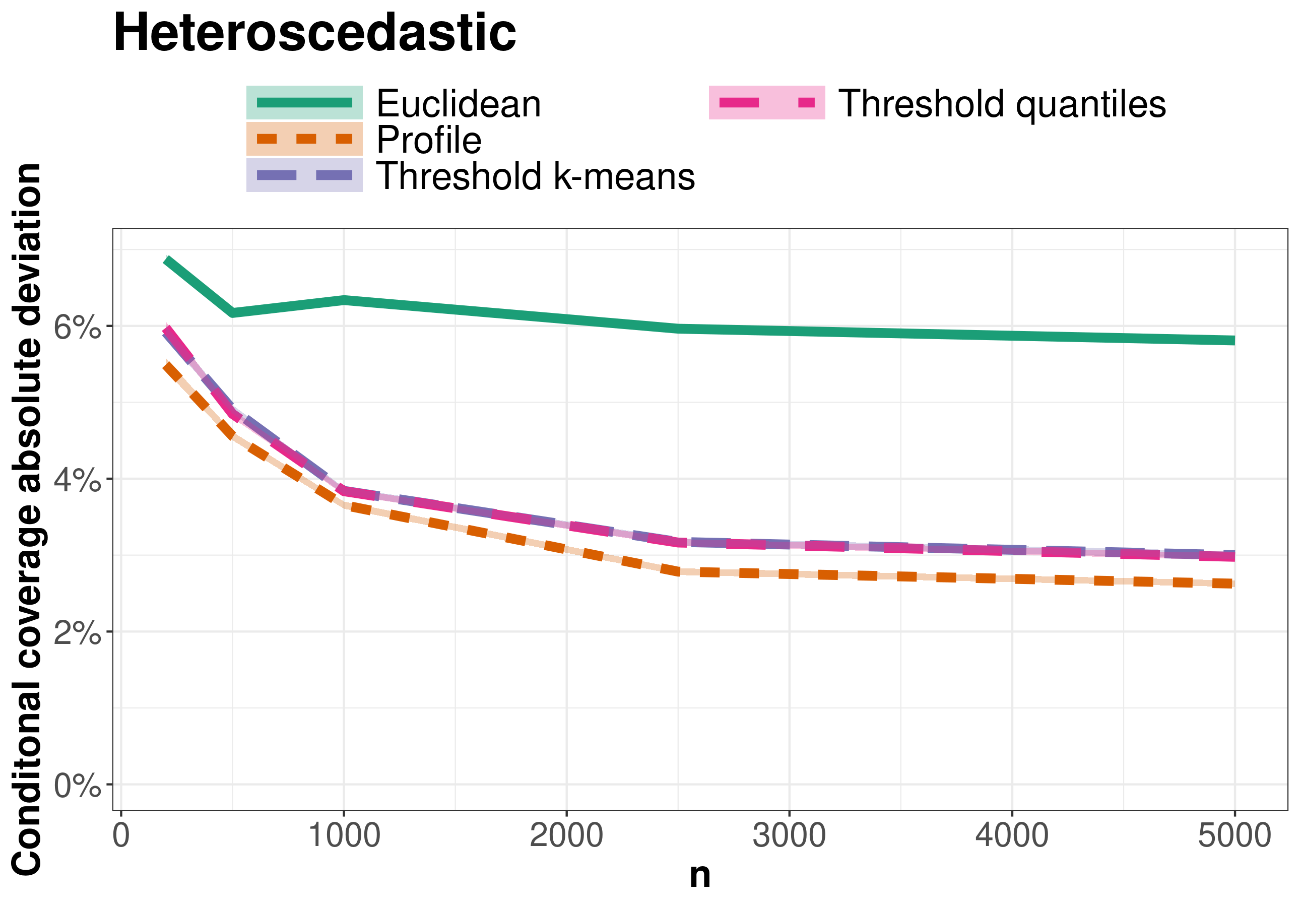
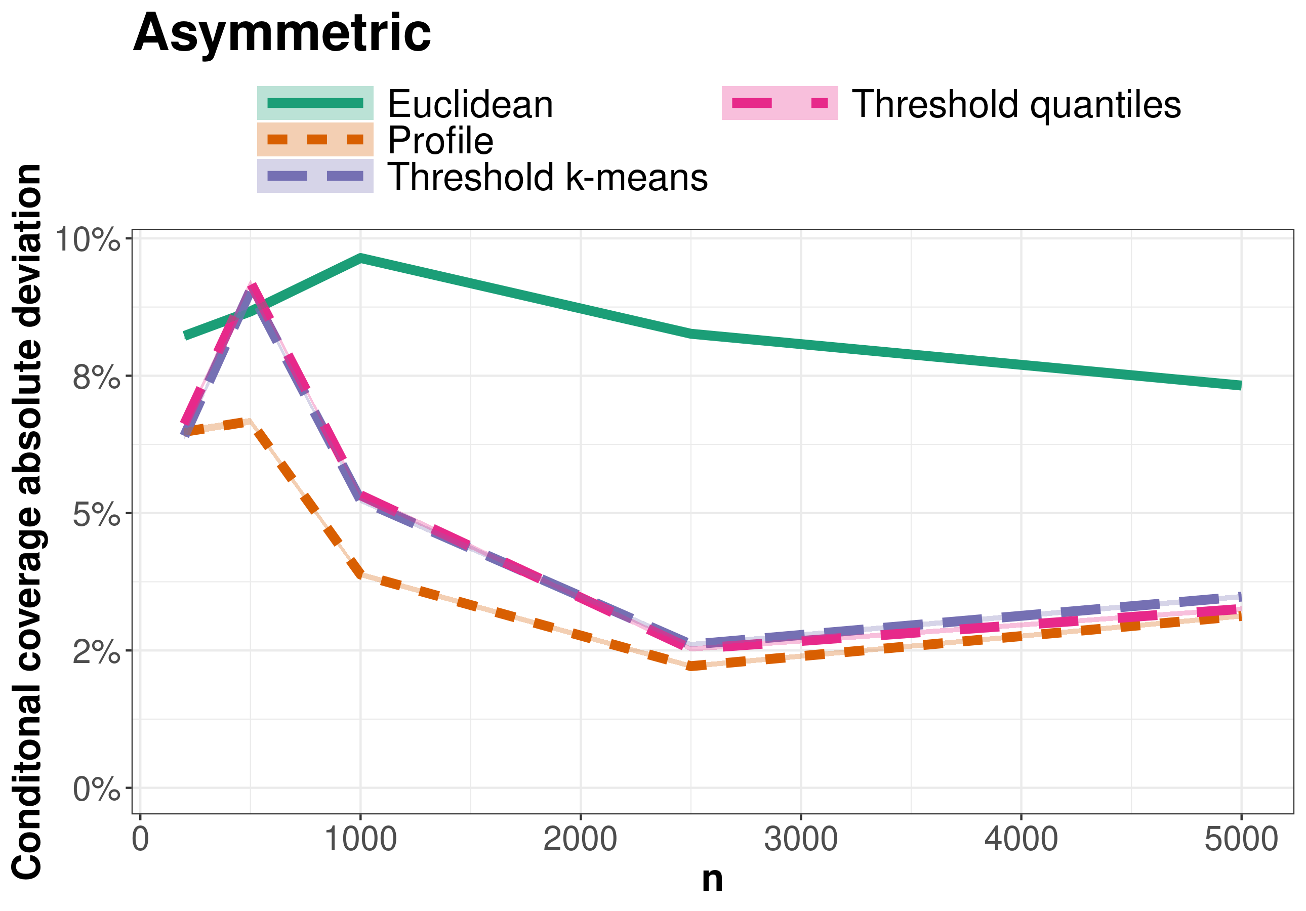
Figure 12: Conditional coverage (top panel) and region size (lower panel) for different partitions in CD-split.

Does the performance of CD-split depend on the choice of the partitions in Definitions 12 and 20? In order to approach this question, we consider some variants of CD-split: Euclidean distance partitions, such as in Lei and Wasserman, (2014) (Euclidean), CD-split with a partition that is induced by intervals of estimated threshold values with the same number of instances (Threshold quantiles), CD-split with a partition chosen according to k-means over the estimated quantiles (Threshold k-means), and the standard CD-split⁺ (Profile). The upper panel of Figure 4 compares these methods according to conditional coverage and region size in the homoscedastic and bimodal scenarios. In the bimodal scenario the Euclidean partition has worse conditional coverage than other partitions and CD-split⁺’s conditional coverage is slightly better than that of threshold methods. The heteroscedastic and asymmetric scenarions behave similarly to the bimodal scenario, as shown in Figure 12 in the Appendix.

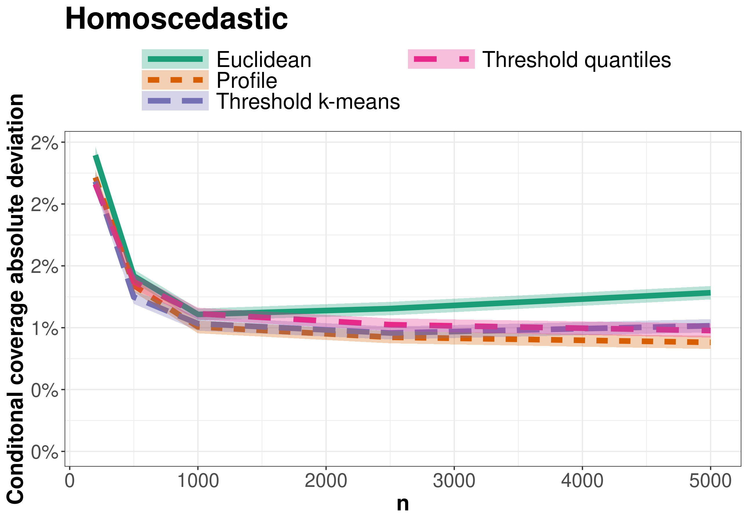
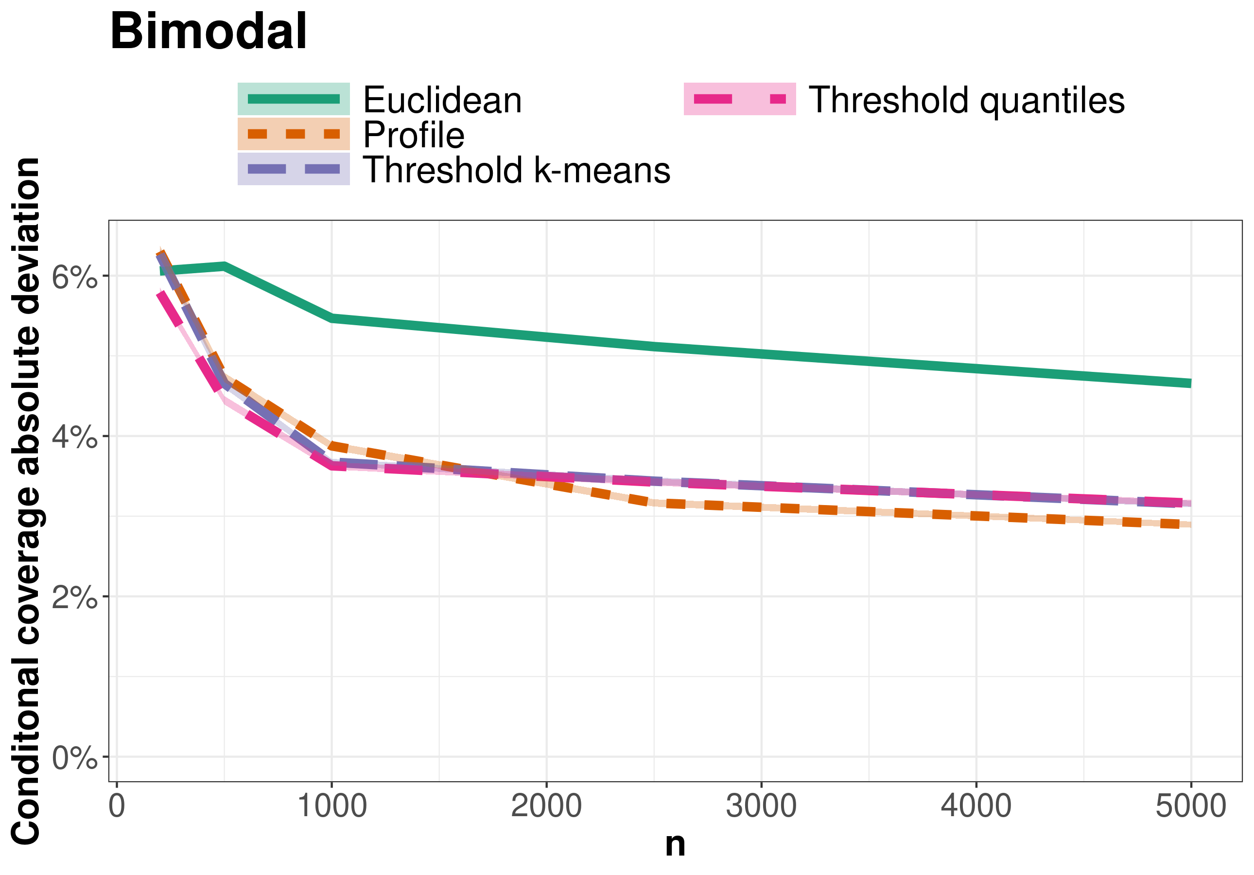
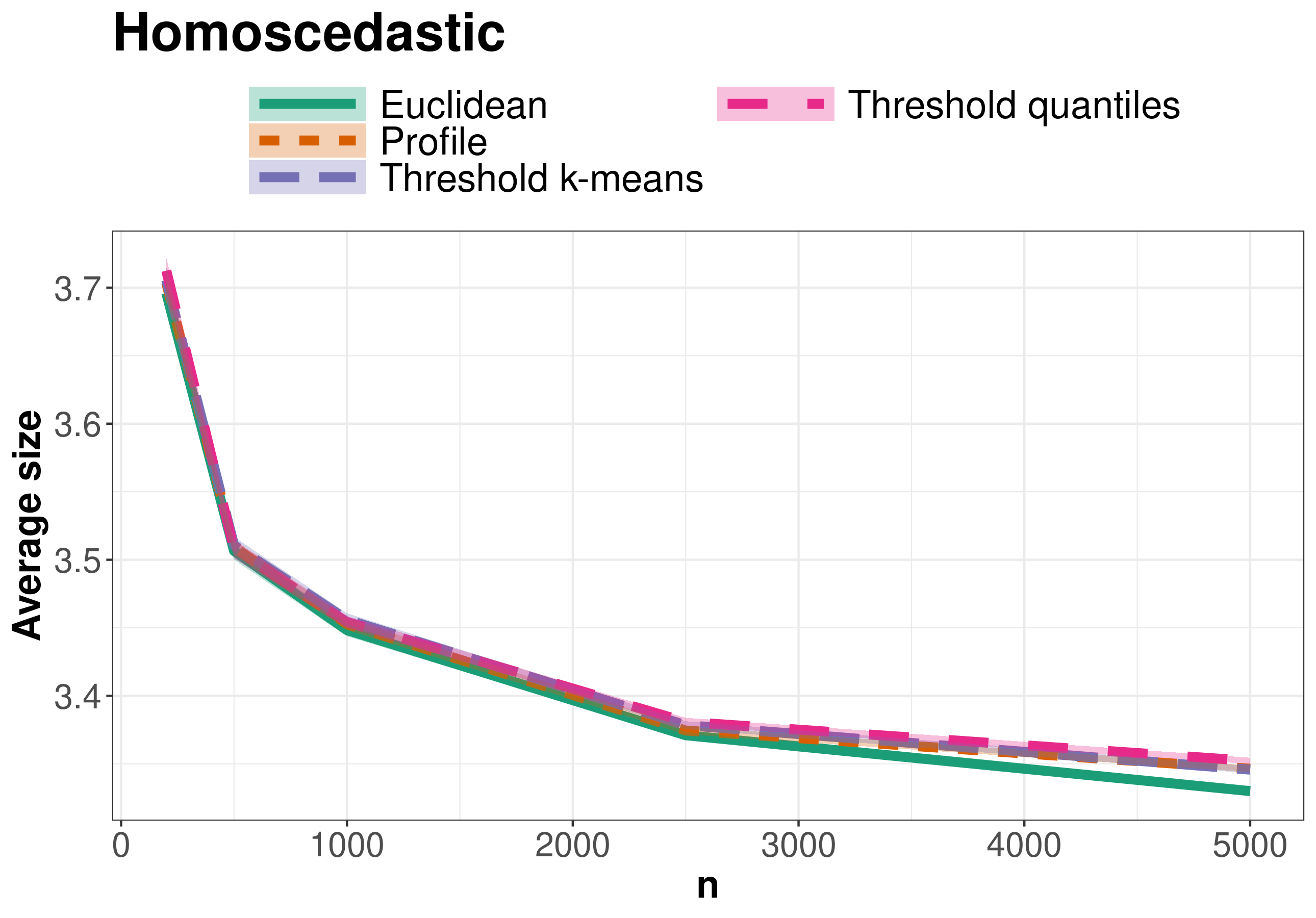
Figure 4: Conditional coverage (top panel) and predictive region size (bottom panel) for different partitions in CD-split.

Besides conditional coverage, one might also wish to compare the above methods according to the expected predictive region size. The lower panel of Figure 4 allows this comparison. Generally, all methods yield similar predictive region sizes. While in homoscedastic scenario all partitions yield similar region sizes, in the bimodal scenario the Euclidean partition yields considerably smaller regions. Figure 12 in the Appendix shows that the asymmetric and heteroscedastic scenarios have similar behaviors. Since the smaller regions in the Euclidean partition come at the cost of a larger conditional coverage deviation, it does not indicate a positive aspect of the Euclidean partition.

The above conclusion can be understood through a simple toy example. Consider that $X\sim\text{Bernoulli}(0.025)$, $Y|X=0\sim N(0,1)$, and $Y|X=1\sim N(0,10^{8})$. In this case, the small predictive region $C_{1}(X)\equiv[-2.25,2.25]$ attains marginal coverage at the expense of conditional coverage. Although $C_{2}(0)=[-2,2]$ and $C_{2}(1)=[-2\cdot 10^{4},2\cdot 10^{4}]$ yields intervals that are much larger on average, the fact that it satisfies conditional coverage makes it better represent the uncertainty about $Y$ given each value of $X$. $C_{2}$ is also the smallest region given $X$.

Given the above considerations, we treat conditional coverage as a primary goal and region size as a secondary goal. Since CD-split⁺ has better conditional coverage than CD-split, we compare only CD-split⁺ to other methods suggested in the literature.

Besides choosing the type of partition, it is also necessary to choose its size. Figure 5 shows how the size of the partition affects the conditional coverage and region size of CD-split⁺ in the homoscedastic and bimodal scenarios. The upper panel shows that in the homoscedastic scenario conditional coverage worsens as the partition size increases. This result is compatible with the fact that, if $f(y|{\mathbf{x}})$ were known, then in this scenario a single partition element would be required (Example 17). On the other hand, in the bimodal scenario conditional coverage decreases until a partition of size $50$ and then it increases. This behavior represents the tradeoff between the number of elements in the partition and how close each element is to ${\mathbf{x}}_{n+1}$. The bottom panels show that, in both scenarios, the region size generally decreases with the partition size. Figure 13 in the Appendix shows that the heteroscedastic and asymmetric scenarios are similar to the bimodal scenario.

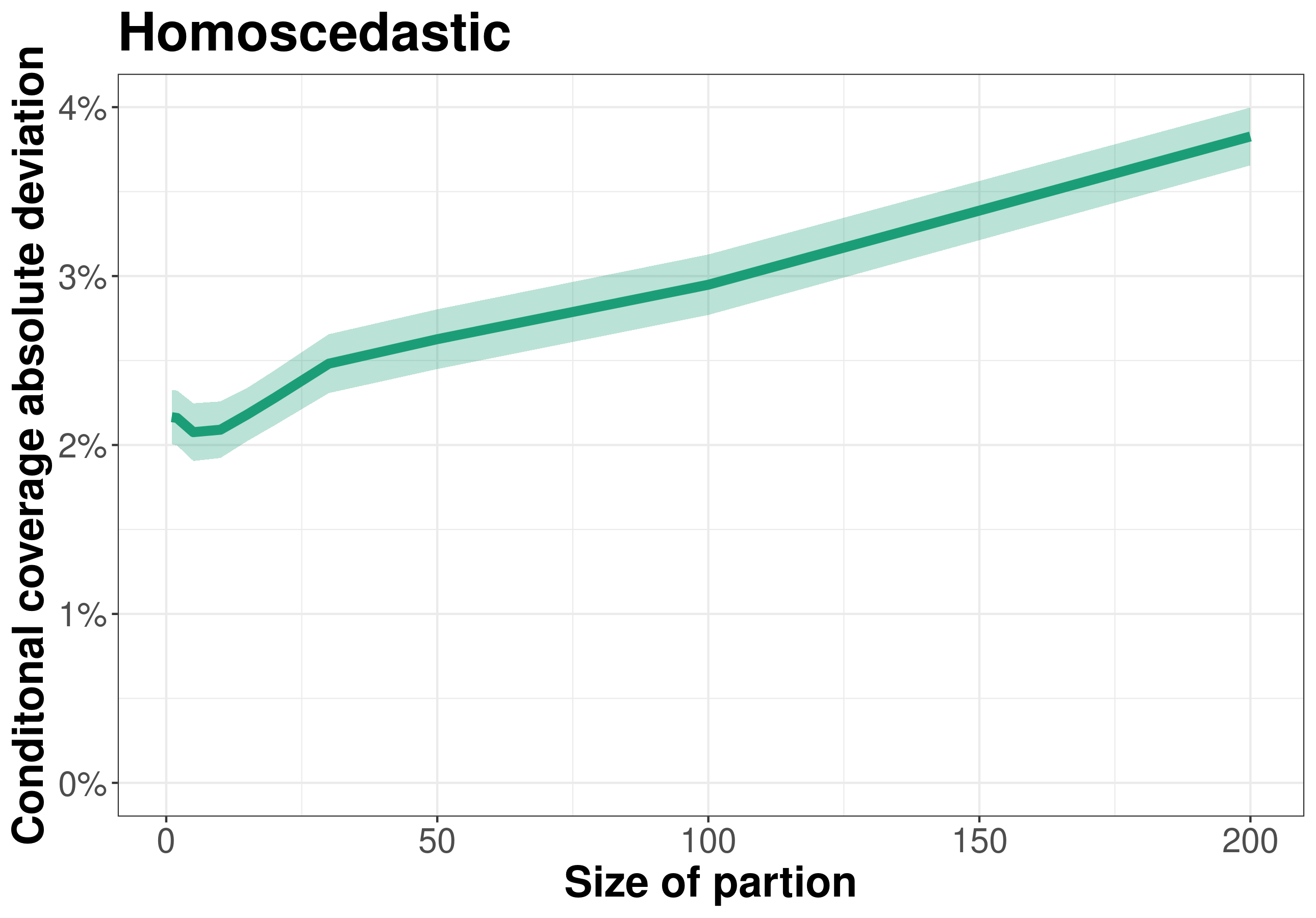
Figure 5: Conditional coverage (top panel) and predictive region size (bottom panel) for different partition sizes in CD-split⁺.

CD-split⁺ also requires tuning with respect to the conditional density estimator. We test this type of tuning by fitting FlexCode coupled with the following regression methods: random forests, knn, and lasso. We also investigate 5 different sample sizes. For each density estimator, we estimated the conditional density loss (CDE loss), $\int\left(\hat{f}(y|{\mathbf{x}})-f(y|{\mathbf{x}})\right)^{2}dP({\mathbf{x}})dy$ (Izbicki and Lee,, 2016). Figure 6 shows that, in homoscedastic and bimodal scenarios, the CDE loss is strongly associated with the conditional coverage and region size of CD-split⁺. That is, conditional density estimates with a smaller loss lead to smaller prediction bands with a better conditional coverage. The only exception occurs in the bimodal scenario, in which although for large sample sizes FlexCode-lasso has a high CDE loss, it also has a small conditional coverage deviation. Figure 14 in the Appendix shows that the heteroscedastic and asymmetric scenarios behave similarly as the bimodal scenario. These observations lead to the conclusion that a practical procedure for obtaining good prediction bands is to choose the conditional density estimator with the smallest estimated CDE loss.

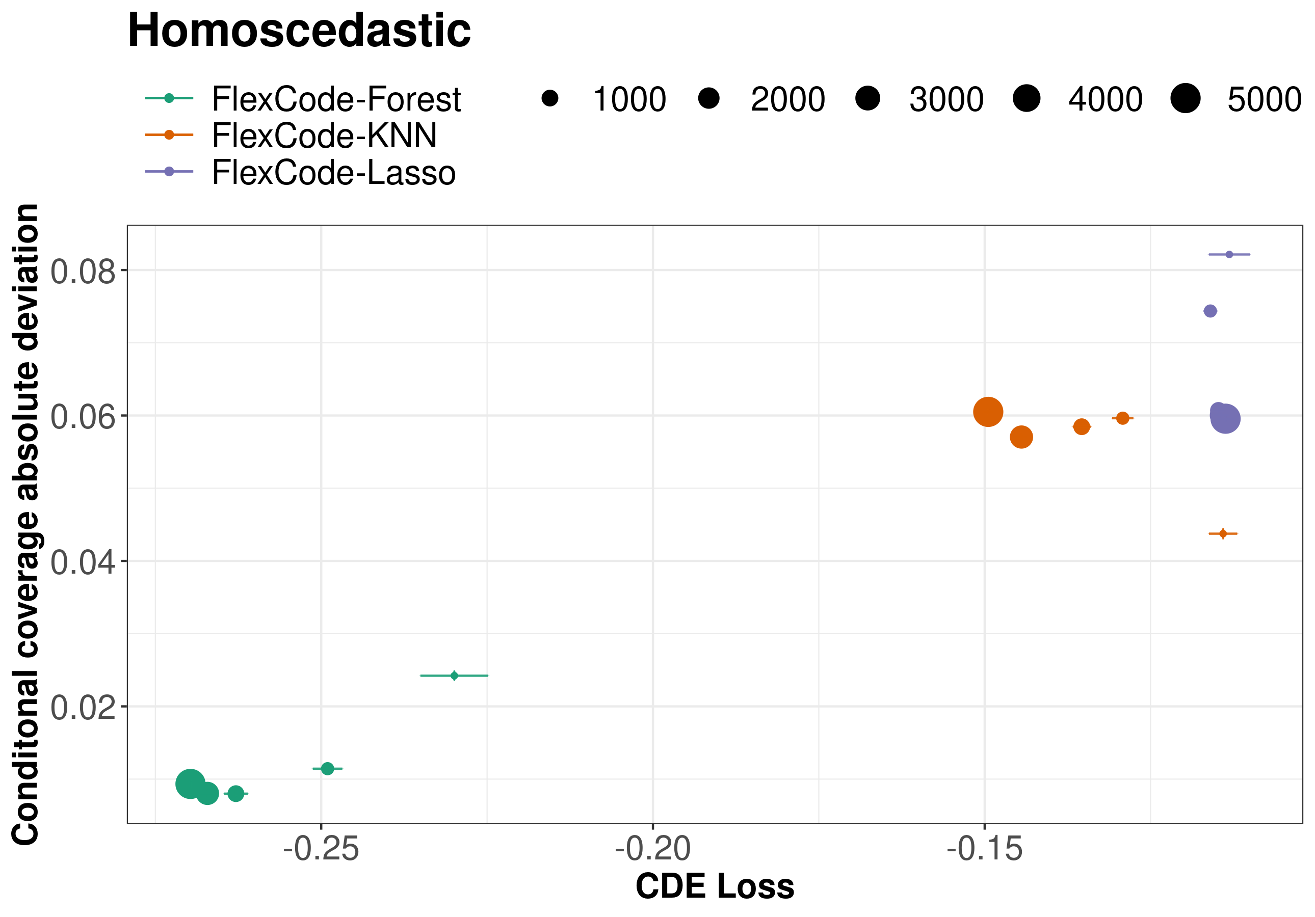
Figure 6: Performance of the CD-split⁺ with respect to conditional coverage (upper panel) and region size (lower panel) as a function of the estimated conditional density loss (CDE loss). Each point is a different combination of sample size and estimator.

5.2 Comparison to Other Conformal Methods

Next, we compare CD-split⁺ and HPD-split to some previously proposed methods:

• [Reg-split] The regression-split method (Lei et al.,, 2018), based on the conformal score $|Y_{i}-\widehat{r}({\mathbf{x}}_{i})|$, where $\widehat{r}$ is an estimate of the regression function.

• [Local Reg-split] The local regression-split method (Lei et al.,, 2018), based on the conformal score $\frac{|Y_{i}-\widehat{r}({\mathbf{x}}_{i})|}{\widehat{\rho}({\mathbf{x}}_{i})}$, where $\widehat{\rho}({\mathbf{x}}_{i})$ is an estimate of the conditional mean absolute deviation of $|Y_{i}-r({\mathbf{x}}_{i})|{\mathbf{x}}_{i}$.

• [Quantile-split] The conformal quantile regression method (Romano et al.,, 2019; Sesia and Candès,, 2019), based on conformalized quantile regression.

• [Dist-split] The conformal method from Izbicki et al., (2020) that uses the cumulative distribution function, $F(y|{\mathbf{x}})$, to create prediction intervals.

• [CD-split⁺] From section 3.3 with partitions of size $\lceil\frac{n}{100}\rceil$.

Each experiment is performed with comparable settings in each method. For instance, random forests (Breiman,, 2001) estimate all required quantities: the regression function in Reg-split, the conditional mean absolute deviation in Local Reg-split, the conditional quantiles via quantile forests (Meinshausen,, 2006) in Quantile-split, and the conditional density via FlexCode (Izbicki and Lee,, 2017) in Dist-split and CD-split⁺. A conditional cumulative distribution estimate, $\widehat{F}(y|{\mathbf{x}})$ is obtained by integrating the conditional density estimate, that is, $\widehat{F}(y|{\mathbf{x}})=\int_{-\infty}^{y}\widehat{f}(y|{\mathbf{x}})dy$. The tuning parameters of all methods were the default of the packages.

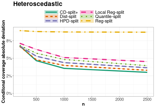
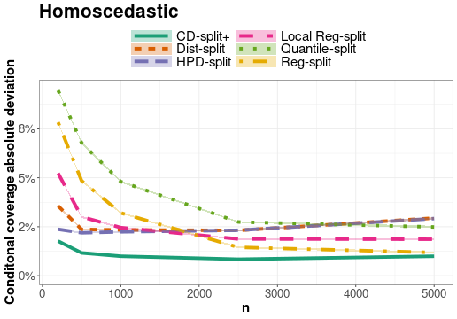
Figure 7: Conditional coverage (left panel) and average size of prediction bands (right panel) for each conformal method as a function of the sample size.

Figure 7 shows the performance of each method as a function of the sample size. While the left side figures display how well each method controls conditional coverage, the right side displays the average size of the obtained predictive regions. Figure 7 shows that, in all settings, CD-split⁺ is the method which best controls conditional coverage. Also, in most cases its prediction bands also have the smallest size. The only exception occurs in the heteroscedastic scenario, in which CD-split⁺ trades a larger prediction band for improved conditional coverage. In general, HPD-split is also very competitive, although it is slightly outperformed in all scenarios by CD-split⁺.

5.3 Effect of dimensionality on performance

How are the CD-split⁺ and HPD-split affected by an increase in the dimension of the feature space? We study this question by fixing the sample size at $n=1000$ and studying the performance of the proposed methods in the scenarios used in the previous sections as the number of irrelevant features increases from $d=0$ to $5000$. These simulations allow a better understanding of the performance of the proposed methods in high-dimensional settings than in the previous sections, in which the number of irrelevant features was fixed at $d=20$.

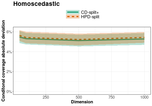
Figure 8: Conditional coverage (left panel) and average size of prediction bands (right panel) for CD-split⁺ and HPD-split as a function of the number of features. None of the methods are heavily affected by increasing dimensionality.

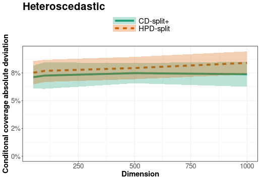
Figure 15: Conditional coverage (left panel) and average size of prediction bands (right panel) for CD-split⁺ and HPD-split as a function of the number of features. None of the methods are heavily affected by increasing dimensionality.

Figure 8 shows that neither CD-split⁺ or HPD-split are heavily affected by the dimensionality of the feature space in the bimodal and homoscedastic scenarios. The same conclusion also applies to the asymmetrical and heteroscedastic scenarios, as shown in fig. 15 in the Appendix. This observation can be explained by the fact that the performance of these methods relies mainly on the quality of the conditional density estimator. In this experiment, this estimation is performed by FlexCode-Random Forest, which automatically performs variable selection. As a result, the density estimates and conformal predictions are reasonable even when there is a large number of irrelevant features, as expected by the empirical and theoretical findings in Izbicki and Lee, (2017).

5.4 Classification

This section studies the performance of CD-split⁺ and HPD-split when applied to conformal classification.

First, a simulation study compares CD-split⁺ and HPD-split to Probability-split (Sadinle et al.,, 2019, Sec. 4.3), a particular case of CD-split⁺ with a unitary partition. We consider that ${\mathbf{X}}=(X_{1},\ldots,X_{d})$, with $X_{i}\overset{\text{iid}}{\sim}N(0,1)$ and $Y|{\mathbf{X}}$ follows the logistic model, ${\mathbb{P}}(Y=i|{\mathbf{x}})\propto\exp\left\{\beta_{i}\cdot x_{1}\right\}$, where $\boldsymbol{\beta}=(-6,-5,-1.5,0,1.5,5,6)$. Figure 9 shows that, while Probability-split can attain slightly smaller predictive bands than the other methods, However, CD-split⁺ yields better conditional coverage as measured by the conditional coverage absolute deviation (top left panel) and also by the size stratified coverage violation (Angelopoulos et al., (2020), bottom panel). In this scenario, HPD-split gives larger prediction bands and does not control conditional coverage as well as the other methods.

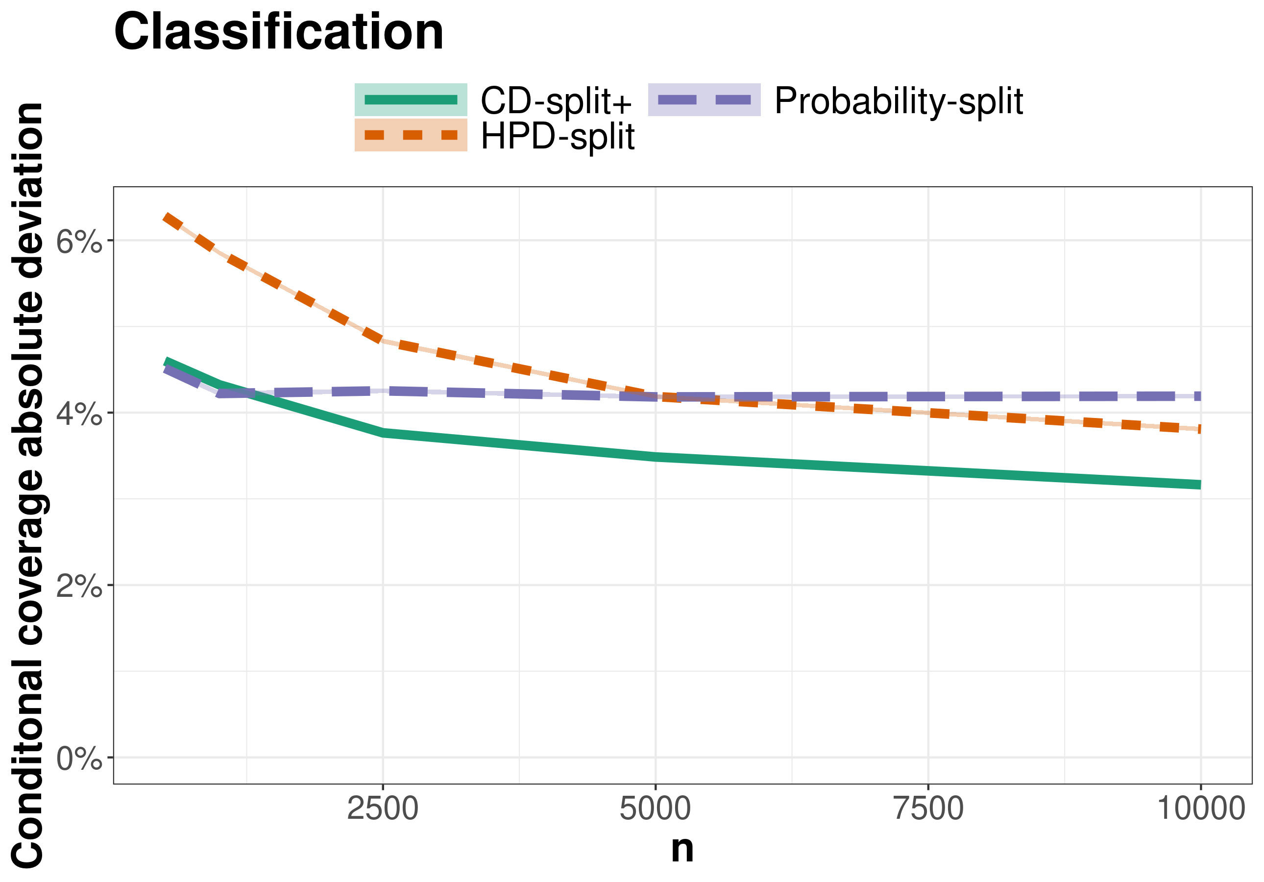
Figure 9: Conditional coverage (top left), average predictive region size (top right), and size stratified coverage violation (SSCV; bottom) of each conformal method as a function of the sample size.

CD-split⁺ and HPD-split are also applied to the MNIST data set (LeCun et al.,, 1995). The data is divided in three sets: 9% as potential future samples, 70% to estimate ${\mathbb{P}}(y|{\mathbf{x}})$, and 21% to calculate split residuals. The conditional density, ${\mathbb{P}}(Y=y|{\mathbf{x}})$, is estimated using a convolutional neural network. Figure 10 shows six examples of images and their respective predictive bands. The top row displays examples where two labels were assigned to each data point. These instances generally seem ambiguous for humans. Both approaches lead to similar results.

Figure 10: Prediction bands given by CD-split⁺ and HPD-split for some instances on MNIST.

6 Application to photometric redshift prediction

We apply CD-split⁺ and HPD-split to a key problem in cosmology: estimating the redshift of a galaxy ($y$) based on its photometric features and $r$-magnitude (${\mathbf{x}}$). This is an important problem since, for instance, redshift is a proxy for the distance between the galaxy and Earth. In this type of problem $f(y|{\mathbf{x}})$ is expected to be highly asymmetrical and often multimodal and, therefore, regression-based predictors are are uninformative (Sheldon et al.,, 2012; Carrasco Kind and Brunner,, 2013; Izbicki et al.,, 2017; Freeman et al.,, 2017). This challenge has motivated the development of several methods for photo-z density estimation (Schmidt et al.,, 2020).

Here we construct prediction bands for redshifts using the Happy A dataset (Beck et al.,, 2017), which is designed to compare photometric redshift prediction algorithms. Happy A contains 74,950 galaxies based on the Sloan Digital Sky Survey DR12. We use 64,950 galaxies as the training set, 5,000 as the prediction set, and 5,000 for comparing the performance of conformal methods. In the training set, the conformity of Reg-split and Quantile-split is fit using random forests. Also, for density-based methods (HPD-split, CD-split⁺ and Dist-split), the conformal score is fit using a Gaussian mixture density neural network (Bishop,, 1994) with three components, one hidden layer and 500 neurons. Using this mixture model, CD-split⁺ and HPD-split yield predictive regions that are the union of at most $3$ intervals. All methods use a marginal coverage level of $1-\alpha=80\%$.

Table 1 shows the local coverage and average size of the prediction bands in two regions of the feature space: bright galaxies and faint galaxies. This classification is based on the galaxy’s $r$-magnitude value: low for bright galaxies and high for faint ones. The table shows that, while on bright galaxies all methods obtain a local coverage close to the nominal 80% level, the same does not happen for faint galaxies. Nominal coverage on faint galaxies is only obtained for HPD-split and CD-split⁺, which therefore better control conditional coverage in this application. The table also shows that, except for Reg-split, all methods yield regions with similar size. Reg-split obtains smaller regions, at the cost of a worse local coverage among faint galaxies.

Figure 11 shows examples of the prediction regions of each method along with an horizontal line indicating the true redshift in each instance. All prediction regions increase in size on faint galaxies since they typically have multimodal densities (Wittman,, 2009; Kügler et al.,, 2016; Polsterer,, 2016; Dalmasso et al.,, 2020). Indeed, in the selected instances of faint galaxies, the true redshift falls either close to $0.25$ or to $0.75$, but never close to $0.5$. This multimodal behavior indicates that the central portion of the prediction intervals obtained in Dist-split and in Quantile-split commonly contains unlikely estimates for the true redshift.

Figure 11: Prediction bands obtained for 5 bright and 5 faint galaxies from the test set. Horizontal lines indicate the true redshift of each galaxy. HPD-split  and CD-split⁺ offer smaller bands than the other methods for faint galaxies (which is where typically $f(z|{\mathbf{x}})$ is multimodal).

Table 1: Coverage and average size of the prediction bands for the photometric redshift prediction problem, along with their standard errors. HPD-split and CD-split⁺ yield smaller prediction sets among the methods that have better control of conditional coverage.

	Galaxy	HPD-split	CD-split+	Dist-split	Quantile-split	Reg-split
Coverage	Bright	0.800 (0.006)	0.795 (0.006)	0.802 (0.006)	0.808 (0.006)	0.807 (0.006)
	Faint	0.788 (0.018)	0.792 (0.018)	0.746 (0.019)	0.754 (0.019)	0.658 (0.021)
Average Size	Bright	0.050 (0.001)	0.049 (0.001)	0.050 (0.001)	0.051 (0.001)	0.044 (0.000)
	Faint	0.065 (0.001)	0.066 (0.001)	0.064 (0.002)	0.074 (0.002)	0.045 (0.000)

7 Final Remarks

We propose two new conformal methods: CD-split and HPD-split. One of the features of these methods is that they can yield arbitrary prediction regions. Therefore, whenever the target variable is for instance multimodal, the proposed prediction regions can be smaller and have better conditional coverage than existing alternatives. Both methods are based on conditional density estimators. Since these estimators are available either when the target variable is discrete (conditional pmf) or continuous (conditional pdf), CD-split and HPD-split provide a unified framework to conformal regression and to conformal classification.

From a theoretical perspective, we provide two types of results. If the instances are exchangeable, then the proposed methods achieve marginal validity and CD-split obtains local validity. Under additional assumptions, such as the consistency of the conditional density estimator, we prove that, even in high-dimensional feature spaces, CD-split obtains asymptotic conditional coverage and converges to the highest predictive density set. Neither of these results require assumptions about the type of dependence between the target variable and the features.

Simulations and applications to real data also point out that the proposed methods perform well. In most of the simulations the proposed methods obtain smaller region sizes and better conditional coverage than other methods in the literature. This high performance occurs both in conformal regression and in conformal classification settings. It is also occurs when the feature is high-dimensional. Furthermore, the proposed methods also yield satisfactory results when predicting photometric redshift. In this application, the target variable is often bimodal. As a result, CD-split and HPD-split yield prediction regions which are often a union of two intervals. These predictions are more informative than the ones obtained by a single interval.

Although CD-split and HPD-split can generally outperform interval-based predictions with respect to region size and conditional coverage, this performance can come at the cost of a more difficult interpretation. It is usually much easier to interpret that the target falls between two values than that it falls in an arbitrary region. A middle ground can be obtained by using, for instance, density estimators based on mixture models, which restrict the prediction regions in CD-split and HPD-split to the union of a fixed number of intervals.

We also show that CD-split can be made more stable by considering different partitions, such as in CD-split⁺. This method is based on a novel data-driven metric on the feature space that defines neighborhoods for conformal methods which perform well even in high-dimensional settings. It might be possible to use this metric with other conformal methods to obtain better conditional coverage.

R code for implementing CD-split, CD-split⁺ and HPD-split is available at:

https://github.com/rizbicki/predictionBands

Appendix A Proofs

The proofs are organized in subsections. Section A.1 proves that convergence to the hpd implies asymptotic conditional validity (Theorem 6). Section A.2 proves all results related to marginal and local validity (Theorems 8, 21 and 22). Section A.3 proves several auxiliary lemmas that are used for proving the asymptotic validity of CD-split, CD-split⁺, and HPD-split. section A.4 proves that HPD-split converges to the hdp set and satisfies asymptotic conditional validity (Theorem 27). Similar results (Theorems 28 and 29) are proved for CD-split and CD-split⁺ respectively in sections A.5 and A.6.

A.1 Proofs of Theorem 6

Lemma 30.

If there exists $C_{\alpha}^{*}({\mathbf{X}}_{n+1})$ such that ${\mathbb{P}}(Y_{n+1}\in C_{\alpha}^{*}({\mathbf{X}}_{n+1})|{\mathbf{X}}_{n+1})\equiv 1-\alpha$ and also such that ${\mathbb{P}}(Y_{n+1}\in C_{\alpha}^{*}({\mathbf{X}}_{n+1})\triangle C_{\alpha}({\mathbf{X}}_{n+1}))=o(1)$, then $C_{\alpha}^{*}({\mathbf{X}}_{n+1})$ satisfies asymptotical conditional validity.

Proof.

Since ${\mathbb{P}}(Y_{n+1}\in C_{\alpha}^{*}({\mathbf{X}}_{n+1})\triangle C_{\alpha}({\mathbf{X}}_{n+1}))=o(1)$, it follows from Markov’s inequality and the dominated convergence theorem that ${\mathbb{P}}(Y_{n+1}\in C_{\alpha}^{*}({\mathbf{X}}_{n+1})\triangle C_{\alpha}({\mathbf{X}}_{n+1})|{\mathbf{X}}_{n_{1}})=o_{{\mathbb{P}}}(1)$. Therefore, there exists $\eta_{n}=o(1)$ such that, for $\Lambda_{n}^{c}=\{{\mathbb{P}}(Y_{n+1}\in C_{\alpha}^{*}({\mathbf{X}}_{n+1})\triangle C_{\alpha}({\mathbf{X}}_{n+1})|{\mathbf{X}}_{n+1})>\eta_{n}\}$, one obtains ${\mathbb{P}}(X_{n}\in\Lambda_{n}^{c})=o(1)$. Conclude that ${\mathbb{P}}(X_{n}\in\Lambda_{n})=1-o(1)$ and that

$$\sup_{{\mathbf{x}}_{n+1}\in{\mathbf{X}}_{n+1}[\Lambda_{n}]}\bigg{|}{\mathbb{P}}(Y_{n+1}\in C_{\alpha}({\mathbf{x}}_{n+1})|{\mathbf{X}}_{n+1}={\mathbf{x}}_{n+1})-1-\alpha\bigg{|}$$

$$\leq \sup_{{\mathbf{x}}_{n+1}\in{\mathbf{X}}_{n+1}[\Lambda_{n}]}\bigg{|}{\mathbb{P}}(Y_{n+1}\in C_{\alpha}^{*}({\mathbf{x}}_{n+1})\triangle C_{\alpha}({\mathbf{x}}_{n+1})|{\mathbf{X}}_{n+1}={\mathbf{x}}_{n+1})\bigg{|}\leq\eta_{n}=o(1)$$

∎

Proof of Theorem 6.

Follows directly from Lemma 30. ∎

A.2 Proofs related to local and marginal validity

Proof of Theorem 8.

Note that $\hat{g}$ is a function of ${\mathbb{D}}^{\prime}$. Therefore, $\hat{g}({\mathbf{X}}_{i},Y_{i})$ can be written as $u({\mathbf{X}}_{i},Y_{i},{\mathbb{D}}^{\prime})$. Since the instances in ${\mathbb{D}}$ are exchangeable, it follows that $U_{i}:=u({\mathbf{X}}_{i},Y_{i},{\mathbb{D}}^{\prime})$ are exchangeable. Therefore, for every $A\in\mathcal{A}$, $\{U_{i}:{\mathbf{X}}_{i}\in A\}$ are exchangeable. In particular, given that ${\mathbf{X}}_{n+1}\in A$, $\{U_{i}:{\mathbf{X}}_{i}\in A({\mathbf{X}}_{n+1})\}$ are exchangeable. That is, for every $A\in\mathcal{A}$,

$${\mathbb{P}}\left(U_{n+1}\geq U_{\lfloor\alpha\rfloor}({\mathbf{X}}_{n+1})|{\mathbf{X}}_{n+1}\in A\right) \geq 1-\alpha$$

$${\mathbb{P}}\left(\hat{g}({\mathbf{X}}_{n+1},Y_{n+1})\geq U_{\lfloor\alpha\rfloor}({\mathbf{X}}_{n+1})|{\mathbf{X}}_{n+1}\in A\right) \geq 1-\alpha$$

$${\mathbb{P}}\left(Y_{n+1}\in\{y:\hat{g}({\mathbf{X}}_{n+1},y)\geq U_{\lfloor\alpha\rfloor}({\mathbf{X}}_{n+1})\}|{\mathbf{X}}_{n+1}\in A\right) \geq 1-\alpha$$

$${\mathbb{P}}(Y_{n+1}\in C({\mathbf{X}}_{n+1})|{\mathbf{X}}_{n+1}\in A) \geq 1-\alpha$$

Conclude that $C({\mathbf{X}}_{n+1})$ satisfies local validity with respect to $\mathcal{A}$ and also satisfies, in particular, marginal validity. ∎

Proof Theorem 21.

Follows directly from Theorem 8. ∎

Proof of Theorem 22.

Follows directly from Theorem 8 by taking $\mathcal{A}=\{{\mathcal{X}}\}$. ∎

A.3 Auxiliary results

Lemma 31.

Under Assumption 24,

$${\mathbb{P}}\left(\sup_{y\in{\mathcal{Y}}}|{\widehat{f}}(y|{\mathbf{X}})-f(y|{\mathbf{X}})|\geq\eta_{n}^{1/3}\right)=o(1).$$

Proof.

Let $B_{n}=\left\{\sup_{y\in{\mathcal{Y}}}|{\widehat{f}}(y|{\mathbf{X}})-f(y|{\mathbf{X}})|\geq\eta_{n}^{1/3}\right\}$ and $A_{n}=\left\{{\mathbb{E}}\left[\sup_{y\in{\mathcal{Y}}}\left({\widehat{f}}(y|{\mathbf{X}})-f(y|{\mathbf{X}})\right)^{2}\big{|}{\widehat{f}}\right]\geq\eta_{n}\right\}$.

$${\mathbb{P}}(B_{n}) ={\mathbb{E}}[{\mathbb{P}}(B_{n}|{\widehat{f}}){\mathbb{I}}(A_{n})]+{\mathbb{E}}[{\mathbb{P}}(B_{n}|{\widehat{f}}){\mathbb{I}}(A_{n}^{c})]$$

$$\leq{\mathbb{P}}(A_{n})+{\mathbb{E}}\left[\frac{{\mathbb{E}}[\sup_{y\in{\mathcal{Y}}}({\widehat{f}}(y|{\mathbf{X}})-f(y|{\mathbf{X}}))^{2}|{\widehat{f}}]}{\eta_{n}^{2/3}}{\mathbb{I}}(A_{n}^{c})\right]$$

$$\leq\rho_{n}+\eta_{n}^{1/3}=o(1)$$

∎

Lemma 32.

Under Assumptions 26, 24 and 25, $\sup_{u}|H(u|{\mathbf{X}}_{i})-{\hat{H}}(u|{\mathbf{X}}_{i})|=o_{{\mathbb{P}}}(1)$. Also, there exists a neighborhood of $\alpha$, $N_{\alpha}$, such that

$$\sup_{u\in N_{\alpha}}\ |H^{-1}(u|{\mathbf{X}}_{i})-{\hat{H}}^{-1}(u|{\mathbf{X}}_{i})|=o_{{\mathbb{P}}}(1).$$

Proof.

Define that $D=\left\{\sup_{y\in{\mathcal{Y}}}|{\widehat{f}}(y|{\mathbf{X}}_{i})-f(y|{\mathbf{X}}_{i})|\geq\eta_{n}^{1/3}\right\}$ and $A_{u}=\left\{y:f(y|{\mathbf{X}}_{i})\leq u,{\widehat{f}}(y|{\mathbf{X}}_{i})\leq u\right\}$. If $D^{c}$ holds, then

$$\sup_{u}\int_{A_{u}}{|f(y|{\mathbf{X}}_{i})-{\widehat{f}}(y|{\mathbf{X}}_{i})|dy} \leq\bigg{|}\int_{{\mathcal{Y}}}\eta_{n}^{1/3}dy\bigg{|} D^{c}$$

$$=o_{\mathbb{P}}(1)$$ (3)

Also let $B_{u}=\{y:f(y|{\mathbf{X}}_{i})\leq u,{\widehat{f}}(y|{\mathbf{X}}_{i})>u\}$. Under $D^{c}$,

$$\sup_{u}\int_{B_{u}}f(y|{\mathbf{X}}_{i})dy \leq\sup_{u}\int_{\{y:u-\eta_{n}^{1/3}\leq f(y|{\mathbf{X}}_{i})\leq u\}}f(y|{\mathbf{X}}_{i})dy D^{c}$$

$$=\sup_{u}|H(u|{\mathbf{X}}_{i})-H(u-\eta_{n}^{1/3}|{\mathbf{X}}_{i})|$$

$$=o_{\mathbb{P}}(1)$$ (4)

Finally, let $C_{u}=\{y:f(y|{\mathbf{X}}_{i})>u,{\widehat{f}}(y|{\mathbf{X}}_{i})\leq u\}$. Under $D^{c}$,

$$\sup_{u}\int_{C_{u}}{\widehat{f}}(y|{\mathbf{X}}_{i})dy \leq\sup_{u}\int_{\{y:u\leq f(y|{\mathbf{X}}_{i})\leq u+\eta_{n}^{1/3}\}}(f(y|{\mathbf{X}}_{i})+\eta_{n}^{1/3})dy D^{c}$$

$$=\sup_{u}|H(u+\eta_{n}^{1/3}|{\mathbf{X}}_{i})-H(u|{\mathbf{X}}_{i})|+o(1)$$

$$o_{\mathbb{P}}(1)$$ (5)

Using the above derivations, observe that under $D^{c}$

$$\sup_{u}|H(u|{\mathbf{X}}_{i})-{\hat{H}}(u|{\mathbf{X}}_{i})| =\sup_{u}\bigg{|}\int_{\{y:f(y|{\mathbf{x}})\leq u\}}{f(y|{\mathbf{x}})dy}-\int_{\{y:{\widehat{f}}(y|{\mathbf{x}})\leq u\}}{{\widehat{f}}(y|{\mathbf{x}})dy}\bigg{|}$$

$$\leq\sup_{u}\int_{A_{u}}{|f(y|{\mathbf{X}}_{i})-{\widehat{f}}(y|{\mathbf{X}}_{i})|dy}+\sup_{u}\int_{B_{u}}f(y|{\mathbf{X}}_{i})dy+\sup_{u}\int_{C_{u}}{\widehat{f}}(y|{\mathbf{X}}_{i})dy$$

$$=o_{\mathbb{P}}(1),\hskip 14.22636pt\text{\lx@cref{creftypeplural~refnum}{eq:cd_dist_1}, \lx@cref{refnum}{eq:cd_dist_2} and \lx@cref{refnum}{eq:cd_dist_3}.}$$

Since Lemma 31 shows that ${\mathbb{P}}(D)=o(1)$, conclude that $\sup_{u}|H(u|{\mathbf{X}}_{i})-{\hat{H}}(u|{\mathbf{X}}_{i})|=o_{{\mathbb{P}}}(1)$. It follows from Assumption 25 that there exists a neighborhood of $\alpha$, $N_{\alpha}$, such that

$$\sup_{u\in N_{\alpha}}\ |H^{-1}(u|{\mathbf{X}}_{i})-{\hat{H}}^{-1}(u|{\mathbf{X}}_{i})|=o_{{\mathbb{P}}}(1).$$

∎

Lemma 33.

Let $C^{*}_{\alpha}=\{y:f(y|{\mathbf{X}}_{n+1})\geq q_{\alpha}({\mathbf{X}}_{n+1})\}$ and $C_{\alpha}=\{y:{\widehat{f}}(y|{\mathbf{X}}_{n+1})\geq\hat{q}_{\alpha}\}$. Under Assumptions 24 and 25, if $|q_{\alpha}({\mathbf{X}}_{n+1})-\hat{q}_{\alpha}|=o_{{\mathbb{P}}}(1)$, then

$${\mathbb{P}}\left(Y\in C^{*}_{\alpha}\triangle C_{\alpha}|{\mathbf{X}}_{n+1}\right)=o_{{\mathbb{P}}}(1)$$

Proof.

Let $B_{n}$ be such as in Lemma 31. It follows from Lemma 31 that ${\mathbb{P}}(B_{n})=o(1)$. Similarly, since $|{q_{\alpha}}-{\hat{q}_{\alpha}}|=o_{\mathbb{P}}(1)$, there exists $\lambda_{n}=o(1)$ such that $D_{n}:={\mathbb{P}}(|{q_{\alpha}}-{\hat{q}_{\alpha}}|>\lambda_{n})=o(1)$. Finally, note that if $E_{n}^{c}:=(B_{n}\cup D_{n})^{c}$ holds, then $C_{\alpha}^{*}\triangle C_{\alpha}\subseteq\{y:|f(y|{\mathbf{X}}_{n+1})-{q_{\alpha}}|\leq\lambda_{n}+\eta_{n}^{1/3}\}$ Therefore,

$${\mathbb{P}}\left(Y_{n+1}\in C_{\alpha}^{*}\triangle C_{\alpha}\right) \leq{\mathbb{P}}\left(Y_{n+1}\in C_{\alpha}^{*}\triangle C_{\alpha},E_{n}^{c}\right)+{\mathbb{P}}(E_{n})$$

$$\leq{\mathbb{P}}(|f(Y_{n+1}|{\mathbf{X}}_{n+1})-{q_{\alpha}}|\leq\lambda_{n}+\eta_{n}^{1/3}\})+o(1)$$

$$={\mathbb{E}}[H({q_{\alpha}}+o(1)|{\mathbf{X}}_{n+1})-H({q_{\alpha}}-o(1)|{\mathbf{X}}_{n+1})]+o(1)$$

$$=o(1) \text{\lx@cref{creftype~refnum}{ass:continuous_hpd}},$$

where the last equality uses the dominated convergence theorem. Since ${\mathbb{P}}\left(Y_{n+1}\in C_{\alpha}^{*}\triangle C_{\alpha}\right)=o(1)$, it follows from Markov’s inequality that ${\mathbb{P}}\left(Y_{n+1}\in C_{\alpha}^{*}\triangle C_{\alpha}|{\mathbf{X}}_{n+1}\right)=o_{\mathbb{P}}(1)$. ∎

A.4 Proof of Theorem 27

Lemma 34.

There exists $\lambda_{n}=o(1)$ such that, under Assumptions 23, 26, 24 and 25, $|I_{1}|=n+o_{\mathbb{P}}(n)$ and $|I_{2}|=o_{\mathbb{P}}(n)$, where $I_{1}:=\left\{i\leq n:|{\hat{H}}({\widehat{f}}(Y_{i}|{\mathbf{X}}_{i}))-H(f(Y_{i}|{\mathbf{X}}_{i}))|\leq\lambda_{n}\right\}$ and $I_{2}=\{1,2,\ldots,n\}-I_{1}$.

Proof.

We start by proving that $\sup_{y}|H(f(y|{\mathbf{X}}_{i}))-{\hat{H}}({\widehat{f}}(y|{\mathbf{X}}_{i}))|=o_{{\mathbb{P}}}(1)$. From the triangular inequality, it is sufficient to show that $\sup_{y}|H(f(y|{\mathbf{X}}_{i}))-H({\widehat{f}}(y|{\mathbf{X}}_{i}))|=o_{{\mathbb{P}}}(1)$ and $\sup_{y}|H({\widehat{f}}(y|{\mathbf{X}}_{i}))-{\hat{H}}({\widehat{f}}(y|{\mathbf{X}}_{i}))|=o_{{\mathbb{P}}}(1)$. From Lemma 31 it follows that $\sup_{y}|f(y|{\mathbf{X}}_{i})-{\widehat{f}}(y|{\mathbf{X}}_{i})|=o_{\mathbb{P}}(1)$ and, therefore, from Assumption 25, $\sup_{y}|H(f(y|{\mathbf{X}}_{i}))-H({\widehat{f}}(y|{\mathbf{X}}_{i}))|=o_{{\mathbb{P}}}(1)$. Also, it follows from Lemma 32 that $\sup_{u}|H(u|{\mathbf{X}}_{i})-{\hat{H}}(u|{\mathbf{X}}_{i})|=o_{{\mathbb{P}}}(1)$ and, therefore, $\sup_{y}|H({\widehat{f}}(y|{\mathbf{X}}_{i}))-{\hat{H}}({\widehat{f}}(y|{\mathbf{X}}_{i}))|=o_{{\mathbb{P}}}(1)$. Conclude that $\sup_{y}|H(f(y|{\mathbf{X}}_{i}))-{\hat{H}}({\widehat{f}}(y|{\mathbf{X}}_{i}))|=o_{{\mathbb{P}}}(1)$.

Next, we show that there exists $\lambda_{n}=o(1)$ such that $|I_{1}|=n+o_{\mathbb{P}}(n)$ and $|I_{2}|=o_{\mathbb{P}}(n)$. Since $\sup_{y}|H(f(y|{\mathbf{X}}_{i}))-{\hat{H}}({\widehat{f}}(y|{\mathbf{X}}_{i}))|=o_{{\mathbb{P}}}(1)$, conclude that $|H(f(Y_{i}|X_{i}))-{\hat{H}}({\widehat{f}}(Y_{i}|X_{i}))|=o_{{\mathbb{P}}}(1)$ and there exists $\lambda_{n}=o(1)$ such that, for $B_{n}:=\{|H(f(Y_{i}|X_{i}))-{\hat{H}}({\widehat{f}}(Y_{i}|X_{i}))|>\lambda_{n}\}$, ${\mathbb{P}}(B_{n})=o(1)$. Therefore, from Assumption 23, $|I_{2}|\sim\text{Binomial}(n,{\mathbb{P}}(B_{n}))$, $|I_{2}|=o_{\mathbb{P}}(n)$, and $|I_{1}|=n+o_{\mathbb{P}}(n)$. ∎

Lemma 35.

Let $U_{i}={\hat{H}}({\widehat{f}}(Y_{i}|{\mathbf{X}}_{i}))$. Under Assumptions 23, 26, 24 and 25, for every $\alpha\in(0,1)$, $U_{\lfloor\alpha\rfloor}=\alpha+o_{P}(1)=U_{\lceil\alpha\rceil}$.

Proof.

Let $I_{1}$ and $I_{2}$ be such as in Lemma 34. Also, let $\hat{G}_{1}$, $G_{1}$ and $G_{0}$ be, the empirical quantiles of, respectively, $\{U_{i}:i\in I_{1}\}$, $\{H(f(Y_{i}|{\mathbf{X}}_{i})):i\in I_{1}\}$, and $\{H(f(Y_{i}|{\mathbf{X}}_{i})):i\leq n\}$. By definition of $I_{1}$, for every $\alpha^{*}\in[0,1]$, $\hat{G}_{1}^{-1}(\alpha^{*})=G_{1}^{-1}(\alpha^{*})+o(1)$. Also, $G_{0}^{-1}(\alpha^{*})=\alpha^{*}+o_{P}(1)$. Therefore, since

$$G_{0}^{-1}\left(\frac{|I_{1}|\alpha^{*}}{n}\right)\leq G_{1}^{-1}(\alpha^{*})\leq G_{0}^{-1}\left(\frac{|I_{1}|\alpha^{*}+|I_{2}|}{n}\right),$$

conclude that $\hat{G}_{1}^{-1}(\alpha^{*})=\alpha^{*}+o_{P}(1)$. Finally, since

$$\hat{G}^{-1}\left(\frac{n\alpha-|I_{2}|}{|I_{1}|}\right)\leq U_{\lfloor\alpha\rfloor}\leq U_{\lceil\alpha\rceil}\leq\hat{G}^{-1}\left(\frac{n\alpha}{|I_{1}|}\right),$$

Conclude that $U_{\lfloor\alpha\rfloor}=\alpha+o_{P}(1)=U_{\lceil\alpha\rceil}$. ∎

Proof of Theorem 27.

First, note that

$$C({\mathbf{X}}_{n+1}) =\left\{y:{\hat{H}}({\widehat{f}}(y|{\mathbf{X}}_{n+1}))\geq U_{\lceil\alpha\rceil}\right\}$$

$$=\left\{y:{\widehat{f}}(y|{\mathbf{X}}_{n+1})\geq{\hat{H}}^{-1}(U_{\lceil\alpha\rceil}|{\mathbf{X}}_{n+1})\right\}.$$ (6)

Note that $q_{\alpha}({\mathbf{x}})=H^{-1}(\alpha|{\mathbf{x}})$ and conclude from Lemmas 35 and 32 that $|{q_{\alpha}}({\mathbf{x}})-{\hat{H}}^{-1}(U_{\lceil\alpha\rceil}|{\mathbf{X}}_{n+1})|=o_{{\mathbb{P}}}(1)$. The proof follows from sections A.4, 33 and 6. ∎

A.5 Proof of Theorem 28

Lemma 36.

Let $M\sim\text{Bin}(n,p)$ and $({\mathbf{X}}_{1},Z_{1})$,…,$({\mathbf{X}}_{M},Z_{M})$ be i.i.d. continuous random variables such that $|F^{-1}_{Z_{i}}(\alpha|{\mathbf{X}}_{i})-t|=o_{{\mathbb{P}}}(1)$ and $F_{Z_{i}}$ is continuous and increasing in a neighborhood of $t$. If ${\widehat{F}}$ is the empirical cdf of $Z_{1},\ldots,Z_{M}$, then $|{\widehat{F}}^{-1}(\alpha)-t|=o_{{\mathbb{P}}}(1)$.

Proof.

Since $|F^{-1}_{Z_{i}}(\alpha|{\mathbf{X}}_{i})-t|=o_{{\mathbb{P}}}(1)$, there exists $\rho_{n}=o(1)$ such that one obtains ${\mathbb{P}}(|F^{-1}_{Z_{i}}(\alpha)-t|>\rho_{n})=o(1)$. Let $A_{n}=\{i\leq M:|F^{-1}_{Z_{i}}(\alpha|{\mathbf{X}}_{i})-t|\leq\rho_{n}\}$, $t_{n}$ be the $\alpha$-quantile of $Z_{i}$ given that $Z_{i}\in A_{n}$, and ${\widehat{F}}_{A}$ be the empirical cumulative distribution function of the $Z_{i}$ in $A_{n}$. By construction,

$${\widehat{F}}_{A}^{-1}\left(\frac{\lfloor(M-|A_{n}^{c}|)\alpha\rfloor}{M}\right)\leq{\widehat{F}}^{-1}\left(\alpha\right)\leq{\widehat{F}}_{A}^{-1}\left(\frac{\lceil M\alpha\rceil}{M}\right).\text{ Therefore, }$$

$${\mathbb{P}}\left(|{\widehat{F}}^{-1}(\alpha)-t|>\epsilon\right) \leq{\mathbb{P}}\left(\max\left(\bigg{|}{\widehat{F}}_{A}^{-1}\left(\frac{\lfloor(M-|A_{n}^{c}|)\alpha\rfloor}{M}\right)-t\bigg{|},\bigg{|}{\widehat{F}}_{A}^{-1}\left(\frac{\lceil M\alpha\rceil}{M}\right)-t\bigg{|}\right)>\epsilon\right)$$

$$\leq{\mathbb{P}}\left(\bigg{|}{\widehat{F}}_{A}^{-1}\left(\frac{\lfloor(M-|A_{n}^{c}|)\alpha\rfloor}{M}\right)-t\bigg{|}\geq 0.5\epsilon\right)+{\mathbb{P}}\left(\bigg{|}{\widehat{F}}_{A}^{-1}\left(\frac{\lceil M\alpha\rceil}{M}\right)-t\bigg{|}>0.5\epsilon\right)$$

Hence, it is enough to show that $\bigg{|}{\widehat{F}}_{A}^{-1}\left(\frac{\lfloor(M-|A_{n}^{c}|)\alpha\rfloor}{M}\right)-t\bigg{|}$ and $\bigg{|}{\widehat{F}}_{A}^{-1}\left(\frac{\lceil M\alpha\rceil}{M}\right)-t\bigg{|}$ are $o_{{\mathbb{P}}}(1)$. Since the proofs are similar, we show only the first case. Furthermore,

$${\mathbb{P}}\left(\bigg{|}{\widehat{F}}_{A}^{-1}\left(\frac{\lfloor(M-|A_{n}^{c}|)\alpha\rfloor}{M}\right)-t\bigg{|}>\epsilon\right) \leq{\mathbb{P}}\left(\bigg{|}{\widehat{F}}_{A}^{-1}\left(\frac{\lfloor(M-|A_{n}^{c}|)\alpha\rfloor}{M}\right)-t_{n}\bigg{|}>\epsilon-|t-t_{n}|\right).$$

It is enough to show that

$${\mathbb{P}}\left({\widehat{F}}_{A}^{-1}\left(\frac{\lfloor(M-|A_{n}^{c}|)\alpha\rfloor}{M}\right)<t_{n}-\epsilon+|t-t_{n}|\right) =o(1)$$ and

$${\mathbb{P}}\left({\widehat{F}}_{A}^{-1}\left(\frac{\lfloor(M-|A_{n}^{c}|)\alpha\rfloor}{M}\right)>t_{n}+\epsilon-|t-t_{n}|\right) =o(1)$$

Since both cases are similar, we show only the former. Note that by construction, $|t-t_{n}|\leq\rho_{n}=o(1)$, and therefore there exists $m_{1}$ such that, for every $n>m_{1}$,

$${\mathbb{P}}\left({\widehat{F}}_{A}^{-1}\left(\frac{\lfloor(M-|A_{n}^{c}|)\alpha\rfloor}{M}\right)<t_{n}-\epsilon+|t-t_{n}|\right) \leq{\mathbb{P}}\left({\widehat{F}}_{A}^{-1}\left(\frac{\lfloor(M-|A_{n}^{c}|)\alpha\rfloor}{M}\right)\leq t_{n}-0.5\epsilon\right)$$

$$\leq{\mathbb{P}}\left(\bigg{|}\left\{i:Z_{i}\in A_{n}\cap Z_{i}\leq t_{n}-0.5\epsilon\right\}\bigg{|}\geq\frac{\lfloor(M-|A_{n}^{c}|)\alpha\rfloor}{M}\cdot|A_{n}|\right)$$

$$={\mathbb{P}}\left(Q_{n}\geq\frac{\lfloor(M-|A_{n}^{c}|)\alpha\rfloor}{M}\cdot|A_{n}|\right),$$ (7)

where $Q_{n}:=\bigg{|}\left\{i:Z_{i}\in A_{n}\cap Z_{i}\leq t_{n}-0.5\epsilon\right\}\bigg{|}$. Let $F_{A}(z):={\mathbb{P}}(Z_{i}\leq y|Z_{i}\in A_{n})$. Since the $Z_{i}$ are i.id., given $A_{n}$, $Q_{n}\sim\text{Binomial}\left(|A_{n}|,F_{A}(t_{n}-0.5\epsilon)\right)$.

It remains to show that $F_{A}(t_{n}-0.5\epsilon)$ is close to $F_{Z_{i}}(t_{n}-0.5\epsilon)$. Since $F_{A}(z)=\frac{{\mathbb{P}}(Z_{i}\leq z\cap Z_{i}\in A_{n})}{{\mathbb{P}}(Z_{i}\in A_{n})}$, obtain $\frac{F_{Z_{i}}(y)-o(1)}{1-o(1)}\leq F_{A}(z)\leq\frac{F_{Z_{i}}(y)}{1-o(1)}$. From these inequalities and observing that $t_{n}=t+o(1)$ and that $F_{Z_{i}}(z)$ is continuous and increasing, conclude that $F_{A}(t_{n}-0.5\epsilon)+o(1)=F_{Z_{i}}(t-0.5\epsilon)<\alpha$. That is, there exists $m_{2}>m_{1}$ such that for $n>m_{2}$, $F_{A}(t_{n}-0.5\epsilon)\leq\alpha_{*}<\alpha$ and, using section A.5,

$${\mathbb{P}}\left(\bigg{|}{\widehat{F}}_{A}^{-1}\left(\frac{\lfloor(M-|A_{n}^{c}|)\alpha\rfloor}{M}\right)-t\bigg{|}>\epsilon\right) \leq{\mathbb{E}}\left[{\mathbb{P}}\left(Q_{n}\geq\frac{\lfloor(M-|A_{n}^{c}|)\alpha\rfloor}{M}\cdot|A_{n}|\bigg{|}A_{n}\right)\right]$$

$$\leq{\mathbb{E}}\left[\exp\left(-2|A_{n}|\left(\alpha^{*}-\frac{\lfloor(M-|A_{n}^{c}|)\alpha\rfloor}{M}\right)^{2}\right)\right]$$

Since ${\mathbb{P}}(M<0.5np)=o(1)$ and $\frac{|A_{n}^{c}|}{M}=o_{{\mathbb{P}}}(1)$, conclude that

$${\mathbb{P}}\left(\bigg{|}{\widehat{F}}_{A}^{-1}\left(\frac{\lfloor(M-|A_{n}^{c}|)\alpha\rfloor}{M}\right)-t\bigg{|}>\epsilon\right) =o(1).$$

∎

Proof of Theorem 28.

Let $Z_{i}={\widehat{f}}(Y_{i}|{\mathbf{X}}_{i})$, $t=H^{-1}(\alpha|{\mathbf{X}}_{n+1})$, and $M=|\mathcal{T}({\mathbf{X}}_{n+1},\mathbb{D})|$. It follows from Assumption 25 that ${\mathbb{P}}({\mathbf{X}}_{i}\in\mathcal{T}({\mathbf{X}}_{n+1},\mathbb{D}))=p>0$. Therefore, $M\sim\text{Bin}(n,p)$. Also, it follows from Lemma 32 that $H^{-1}(\alpha|{\mathbf{X}}_{i})-{\hat{H}}^{-1}(\alpha|{\mathbf{X}}_{i})=o_{{\mathbb{P}}}(1)$. Therefore, for every ${\mathbf{X}}_{i}\in A({\mathbf{X}}_{n+1})$, $H^{-1}(\alpha|{\mathbf{X}}_{i})-t=o_{{\mathbb{P}}}(1)$, that is, $F^{-1}_{Z_{i}}(\alpha)-t=o_{{\mathbb{P}}}(1)$. Since $U_{\lfloor\alpha\rfloor}({\mathbf{X}}_{n+1})$ is the $\alpha$-quantile of the empirical cdf of $\{Z_{i}:i\in A({\mathbf{X}}_{n+1})\}$, conclude from Lemma 36 that $|U_{\lfloor\alpha\rfloor}({\mathbf{X}}_{n+1})-t|=o_{{\mathbb{P}}}(1)$. The rest of the proof follows directly from Lemmas 33 and 6. ∎

A.6 Proof of Theorem 29

Lemma 37.

Under Assumptions 26 and 25, there exist a universal constants, $C_{1}$, such that, for every ${\mathbf{x}}_{0},{\mathbf{x}}_{1}\in{\mathcal{X}}$, $C_{1}\|H(\cdot|{\mathbf{x}}_{0})-H(\cdot|{\mathbf{x}}_{1})\|_{\infty}^{1.5}\leq\|H(\cdot|{\mathbf{x}}_{0})-H(\cdot|{\mathbf{x}}_{1})\|_{2}$. Furthermore, if ${\hat{H}}$ has the same support as $H$ and $\|{\hat{H}}\|_{\infty}<1$, then there exists a universal constant, $C_{2}$, such that $\|H(\cdot|{\mathbf{x}}_{0})-{\hat{H}}(\cdot|{\mathbf{x}}_{1})\|_{2}\leq C_{2}\|H(\cdot|{\mathbf{x}}_{0})-{\hat{H}}(\cdot|{\mathbf{x}}_{1})\|_{\infty}^{0.5}$.

Proof.

Let $z:=0.5\|H(\cdot|{\mathbf{x}}_{0})-H(\cdot|{\mathbf{x}}_{1})\|_{\infty}$ and $y^{*}$ be such that $|H(y^{*}|{\mathbf{x}}_{0})-H(y^{*}|{\mathbf{x}}_{1})|\geq z$. It follows from Assumption 25 that $H(\cdot|{\mathbf{x}}_{0})-H(\cdot|{\mathbf{x}}_{1})$ is Lipschitz continuous and, in particular, for every $y\in\left[y^{*}-z(2M)^{-1},y^{*}+z(2M)^{-1}\right]$, $|H(y|{\mathbf{x}}_{0})-H(y|{\mathbf{x}}_{1})|\geq z-2M|y^{*}-y|$. Therefore, there exists $C_{1}$ such that $\|H(\cdot|{\mathbf{x}}_{0})-H(\cdot|{\mathbf{x}}_{1})\|_{2}\geq C_{1}\|H(\cdot|{\mathbf{x}}_{0})-H(\cdot|{\mathbf{x}}_{1})\|_{\infty}^{1.5}$.

Next, since $|H|$ and $|{\hat{H}}|$ are bounded by $1$, $\|H(\cdot|{\mathbf{x}}_{0})-H(\cdot|{\mathbf{x}}_{1})\|_{1}\leq 2|{\mathcal{Y}}|$. Therefore,

$$\|H(\cdot|{\mathbf{x}}_{0})-H(\cdot|{\mathbf{x}}_{1})\|_{2}^{2} \leq\|H(\cdot|{\mathbf{x}}_{0})-H(\cdot|{\mathbf{x}}_{1})\|_{1}\cdot\|H(\cdot|{\mathbf{x}}_{0})-H(\cdot|{\mathbf{x}}_{1})\|_{\infty}$$ Hölders inequality

$$\leq 2|{\mathcal{Y}}|\cdot\|H(\cdot|{\mathbf{x}}_{0})-H(\cdot|{\mathbf{x}}_{1})\|_{\infty}.$$

The proof follows directly from Assumption 26. ∎

Lemma 38.

Under Assumptions 23, 26, 24 and 25, if $\|{\hat{H}}(\cdot|{\mathbf{X}}_{i})-{\hat{H}}(\cdot|{\mathbf{X}}_{n+1})\|_{2}=o(1)$, then

$${\hat{H}}^{-1}(\alpha|{\mathbf{X}}_{i})-H^{-1}(\alpha|{\mathbf{X}}_{n+1})=o_{\mathbb{P}}(1).$$

Proof.

It follows from Lemma 32 that $H^{-1}(\alpha|{\mathbf{X}}_{i})-{\hat{H}}^{-1}(\alpha|{\mathbf{X}}_{i})=o_{\mathbb{P}}(1)$ and, therefore, it is sufficient to prove that $H^{-1}(\alpha|{\mathbf{X}}_{i})-H^{-1}(\alpha|{\mathbf{X}}_{n+1})=o_{\mathbb{P}}(1)$. Note that

$$\|H(\cdot|{\mathbf{X}}_{i})-H(\cdot|{\mathbf{X}}_{n+1})\|_{2}\leq \|H(\cdot|{\mathbf{X}}_{i})-{\hat{H}}(\cdot|{\mathbf{X}}_{i})\|_{2}+\|{\hat{H}}(\cdot|{\mathbf{X}}_{i})-{\hat{H}}(\cdot|{\mathbf{X}}_{n+1})\|_{2}$$

$$+\|{\hat{H}}(\cdot|{\mathbf{X}}_{n+1})-H(\cdot|{\mathbf{X}}_{n+1})\|_{2}$$

$$\leq C_{2}(\|H(\cdot|{\mathbf{X}}_{i})-{\hat{H}}(\cdot|{\mathbf{X}}_{i})\|_{\infty}^{0.5}+\|H(\cdot|{\mathbf{X}}_{n+1})-{\hat{H}}(\cdot|{\mathbf{X}}_{n+1})\|_{\infty}^{0.5})+o(1)$$

$$=o_{{\mathbb{P}}}(1)$$

Conclude from Lemma 37 that $\|H(\cdot|{\mathbf{X}}_{i})-H(\cdot|{\mathbf{X}}_{n+1})\|_{\infty}=o_{\mathbb{P}}(1)$. It follows from Assumption 25 that $H^{-1}(\alpha|{\mathbf{X}}_{i})-H^{-1}(\alpha|{\mathbf{X}}_{n+1})=o_{\mathbb{P}}(1)$, which completes the proof. ∎

Proof of Theorem 29.

Let $Z_{i}={\widehat{f}}(Y_{i}|{\mathbf{X}}_{i})$, $t=H^{-1}(\alpha|{\mathbf{X}}_{n+1})$, and $M=|\mathcal{T}({\mathbf{X}}_{n+1},\mathbb{D})|$. It follows from Assumption 25 that ${\mathbb{P}}({\mathbf{X}}_{i}\in\mathcal{T}({\mathbf{X}}_{n+1},\mathbb{D}))=p>0$. Therefore, $M\sim\text{Bin}(n,p)$. Also, it follows from Lemma 38 that, for every ${\mathbf{X}}_{i}\in A({\mathbf{x}}_{n+1})$, $H^{-1}(\alpha|{\mathbf{X}}_{i})-t=o_{{\mathbb{P}}}(1)$, that is, $F^{-1}_{Z_{i}}(\alpha)-t=o_{{\mathbb{P}}}(1)$. Since $U_{\lfloor\alpha\rfloor}({\mathbf{X}}_{n+1})$ is the $\alpha$-quantile of the empirical cdf of $\{Z_{i}:i\in A({\mathbf{X}}_{n+1})\}$, conclude from Lemma 36 that $|U_{\lfloor\alpha\rfloor}({\mathbf{X}}_{n+1})-t|=o_{{\mathbb{P}}}(1)$. The rest of the proof follows directly from Lemmas 33 and 6 ∎

Appendix B. Additional figures

Figure 13: Conditional coverage (top panel) and predictive region size (bottom panel) for different partition sizes in CD-split⁺.

Figure 14: Performance of the CD-split⁺ with respect to conditional coverage (upper panel) and region size (lower panel) as a function of the estimated conditional density loss (CDE loss). Each point is a different combination of sample size and estimator.

References

• Angelopoulos et al., (2020) Angelopoulos, A. N., Bates, S., Jordan, M., and Malik, J. (2020). Uncertainty sets for image classifiers using conformal prediction. In International Conference on Learning Representations.
• Arthur and Vassilvitskii, (2007) Arthur, D. and Vassilvitskii, S. (2007). k-means++: The advantages of careful seeding. In Proceedings of the eighteenth annual ACM-SIAM symposium on Discrete algorithms, pages 1027–1035. Society for Industrial and Applied Mathematics.
• Barber et al., (2019) Barber, R. F., Candès, E. J., Ramdas, A., and Tibshirani, R. J. (2019). The limits of distribution-free conditional predictive inference. arXiv preprint arXiv:1903.04684.
• Beck et al., (2017) Beck, R., Lin, C.-A., Ishida, E., Gieseke, F., de Souza, R., Costa-Duarte, M., Hattab, M., Krone-Martins, A., and Collaboration, C. (2017). On the realistic validation of photometric redshifts. Monthly Notices of the Royal Astronomical Society, 468(4):4323–4339.
• Bishop, (1994) Bishop, C. M. (1994). Mixture density networks.
• Breiman, (2001) Breiman, L. (2001). Random forests. Machine learning, 45(1):5–32.
• Carrasco Kind and Brunner, (2013) Carrasco Kind, M. and Brunner, R. J. (2013). Tpz: photometric redshift pdfs and ancillary information by using prediction trees and random forests. Monthly Notices of the Royal Astronomical Society, 432(2):1483–1501.
• Cauchois et al., (2021) Cauchois, M., Gupta, S., and Duchi, J. C. (2021). Knowing what you know: valid and validated confidence sets in multiclass and multilabel prediction. Journal of Machine Learning Research, 22(81):1–42.
• Chernozhukov et al., (2019) Chernozhukov, V., Wüthrich, K., and Zhu, Y. (2019). Distributional conformal prediction. arXiv preprint arXiv:1909.07889.
• Dalmasso et al., (2020) Dalmasso, N., Pospisil, T., Lee, A. B., Izbicki, R., Freeman, P. E., and Malz, A. I. (2020). Conditional density estimation tools in python and r with applications to photometric redshifts and likelihood-free cosmological inference. Astronomy and Computing, 30:100362.
• De Gooijer and Zerom, (2003) De Gooijer, J. G. and Zerom, D. (2003). On conditional density estimation. Statistica Neerlandica, 57(2):159–176.
• Dutordoir et al., (2018) Dutordoir, V., Salimbeni, H., Hensman, J., and Deisenroth, M. (2018). Gaussian process conditional density estimation. In Bengio, S., Wallach, H., Larochelle, H., Grauman, K., Cesa-Bianchi, N., and Garnett, R., editors, Advances in Neural Information Processing Systems, volume 31. Curran Associates, Inc.
• Freeman et al., (2017) Freeman, P. E., Izbicki, R., and Lee, A. B. (2017). A unified framework for constructing, tuning and assessing photometric redshift density estimates in a selection bias setting. Monthly Notices of the Royal Astronomical Society, 468(4):4556–4565.
• Guan, (2019) Guan, L. (2019). Conformal prediction with localization. arXiv preprint arXiv:1908.08558.
• Hyndman et al., (1996) Hyndman, R. J., Bashtannyk, D. M., and Grunwald, G. K. (1996). Estimating and visualizing conditional densities. Journal of Computational and Graphical Statistics, 5(4):315–336.
• Izbicki and Lee, (2016) Izbicki, R. and Lee, A. B. (2016). Nonparametric conditional density estimation in a high-dimensional regression setting. Journal of Computational and Graphical Statistics, 25(4):1297–1316.
• Izbicki and Lee, (2017) Izbicki, R. and Lee, A. B. (2017). Converting high-dimensional regression to high-dimensional conditional density estimation. Electronic Journal of Statistics, 11(2):2800–2831.
• Izbicki et al., (2017) Izbicki, R., Lee, A. B., and Freeman, P. E. (2017). Photo-$z$ estimation: An example of nonparametric conditional density estimation under selection bias. The Annals of Applied Statistics, 11(2):698–724.
• Izbicki et al., (2020) Izbicki, R., Shimizu, G., and Stern, R. B. (2020). Distribution-free conditional predictive bands using density estimators. In Proceedings of AISTATS 2020, volume 108, pages 3068–3077.
• Kallenberg, (2006) Kallenberg, O. (2006). Probabilistic symmetries and invariance principles. Springer Science & Business Media.
• Kügler et al., (2016) Kügler, S. D., Gianniotis, N., and Polsterer, K. L. (2016). A spectral model for multimodal redshift estimation. In 2016 IEEE Symposium Series on Computational Intelligence (SSCI), pages 1–8. IEEE.
• LeCun et al., (1995) LeCun, Y., Jackel, L., Bottou, L., Brunot, A., Cortes, C., Denker, J., Drucker, H., Guyon, I., Muller, U., Sackinger, E., et al. (1995). Comparison of learning algorithms for handwritten digit recognition. In International conference on artificial neural networks, volume 60, pages 53–60. Perth, Australia.
• Lei et al., (2018) Lei, J., G’Sell, M., Rinaldo, A., Tibshirani, R. J., and Wasserman, L. (2018). Distribution-free predictive inference for regression. Journal of the American Statistical Association, 113(523):1094–1111.
• Lei and Wasserman, (2014) Lei, J. and Wasserman, L. (2014). Distribution-free prediction bands for non-parametric regression. Journal of the Royal Statistical Society: Series B (Statistical Methodology), 76(1):71–96.
• Meinshausen, (2006) Meinshausen, N. (2006). Quantile regression forests. Journal of Machine Learning Research, 7(Jun):983–999.
• Neter et al., (1996) Neter, J., Kutner, M. H., Nachtsheim, C. J., and Wasserman, W. (1996). Applied linear statistical models, volume 4. Irwin Chicago.
• Papadopoulos et al., (2002) Papadopoulos, H., Proedrou, K., Vovk, V., and Gammerman, A. (2002). Inductive confidence machines for regression. In European Conference on Machine Learning, pages 345–356. Springer.
• Polsterer, (2016) Polsterer, K. L. (2016). Dealing with uncertain multimodal photometric redshift estimations. Proceedings of the International Astronomical Union, 12(S325):156–165.
• Romano et al., (2019) Romano, Y., Patterson, E., and Candès, E. J. (2019). Conformalized quantile regression.
• Romano et al., (2020) Romano, Y., Sesia, M., and Candes, E. (2020). Classification with valid and adaptive coverage. Advances in Neural Information Processing Systems, 33:3581–3591.
• Sadinle et al., (2019) Sadinle, M., Lei, J., and Wasserman, L. (2019). Least ambiguous set-valued classifiers with bounded error levels. Journal of the American Statistical Association, 114(525):223–234.
• Schmidt et al., (2020) Schmidt, S., Malz, A., Soo, J., Almosallam, I., Brescia, M., Cavuoti, S., Cohen-Tanugi, J., Connolly, A., DeRose, J., Freeman, P., et al. (2020). Evaluation of probabilistic photometric redshift estimation approaches for the rubin observatory legacy survey of space and time (lsst). Monthly Notices of the Royal Astronomical Society, 499(2):1587–1606.
• Sesia and Candès, (2019) Sesia, M. and Candès, E. J. (2019). A comparison of some conformal quantile regression methods. arXiv preprint arXiv:1909.05433.
• Sheldon et al., (2012) Sheldon, E. S., Cunha, C. E., Mandelbaum, R., Brinkmann, J., and Weaver, B. A. (2012). Photometric redshift probability distributions for galaxies in the sdss dr8. The Astrophysical Journal Supplement Series, 201(2):32.
• Tibshirani et al., (2019) Tibshirani, R. J., Barber, R. F., Candès, E. J., and Ramdas, A. (2019). Conformal prediction under covariate shift. In Proceedings of the 33rd International Conference on Neural Information Processing Systems, pages 2530–2540.
• Vovk, (2012) Vovk, V. (2012). Conditional validity of inductive conformal predictors. In Asian conference on machine learning, pages 475–490.
• Vovk et al., (2005) Vovk, V. et al. (2005). Algorithmic learning in a random world. Springer Science & Business Media.
• Vovk et al., (2009) Vovk, V., Nouretdinov, I., Gammerman, A., et al. (2009). On-line predictive linear regression. The Annals of Statistics, 37(3):1566–1590.
• Wittman, (2009) Wittman, D. (2009). What lies beneath: Using p (z) to reduce systematic photometric redshift errors. The Astrophysical Journal Letters, 700(2):L174.