Feynman checkers:
towards algorithmic quantum theory

Abstract

We survey and develop the most elementary model of electron motion introduced by R.Feynman. In this game, a checker moves on a checkerboard by simple rules, and we count the turns. Feynman checkers are also known as a one-dimensional quantum walk or an Ising model at imaginary temperature. We solve mathematically a problem by R.Feynman from 1965, which was to prove that the discrete model (for large time, small average velocity, and small lattice step) is consistent with the continuum one. We study asymptotic properties of the model (for small lattice step and large time) improving the results by J.Narlikar from 1972 and by T.Sunada–T.Tate from 2012. For the first time we observe and prove concentration of measure in the small-lattice-step limit. We perform the second quantization of the model.

Keywords and phrases. Feynman checkerboard, quantum walk, Ising model, Young diagram, Dirac equation, stationary phase method

MSC2010: 82B20, 11L03, 68Q12, 81P68, 81T25, 81T40, 05A17, 11P82, 33C45.

1 Introduction

We survey and develop the most elementary model of electron motion introduced by R. Feynman (see Figure 1). In this game, a checker moves on a checkerboard by simple rules, and we count the turns (see Definition 2). Feynman checkers can be viewed as a one-dimensional quantum walk, or an Ising model, or count of Young diagrams of certain type.

Figure 1: The probability to find an electron in a small square around a given point (white depicts strong oscillations of the probability). Left: in the basic model from §2 (cf. [51, Figure 6]). Middle: in the upgrade from §3 for smaller square side. Right: in continuum theory. For the latter, the relative probability density is depicted.

1.1 Motivation

The simplest way to understand what is the model about is the classical double-slit experiment (see Figure 2). In this experiment, a (coherent) beam of electrons is directed towards a plate pierced by two parallel slits, and the part of the beam passing through the slits is observed on a screen behind the plate. If one of the slits is closed, then the beam illuminates a spot on the screen. If both slits are open, one would expect a larger spot, but in fact one observes a sequence of bright and dark bands (interferogram).

This shows that electrons behave like a wave: the waves travel through both slits, and the contributions of the two paths either amplify or cancel each other depending on the final phases.

Further, if the electrons are sent through the slits one at time, then single dots appear on the screen, as expected. Remarkably, however, the same interferogram with bright and dark bands emerges when the electrons are allowed to build up one by one. One cannot predict where a particular electron hits the screen; all we can do is to compute the probability to find the electron at a given place.

The Feynman sum-over-paths (or path integral) method of computing such probabilities is to assign phases to all possible paths and to sum up the resulting waves (see [11, 12]). Feynman checkers (or Feynman checkerboard) is a particularly simple combinatorial rule for those phases in the case of an electron freely moving (or better jumping) along a line.

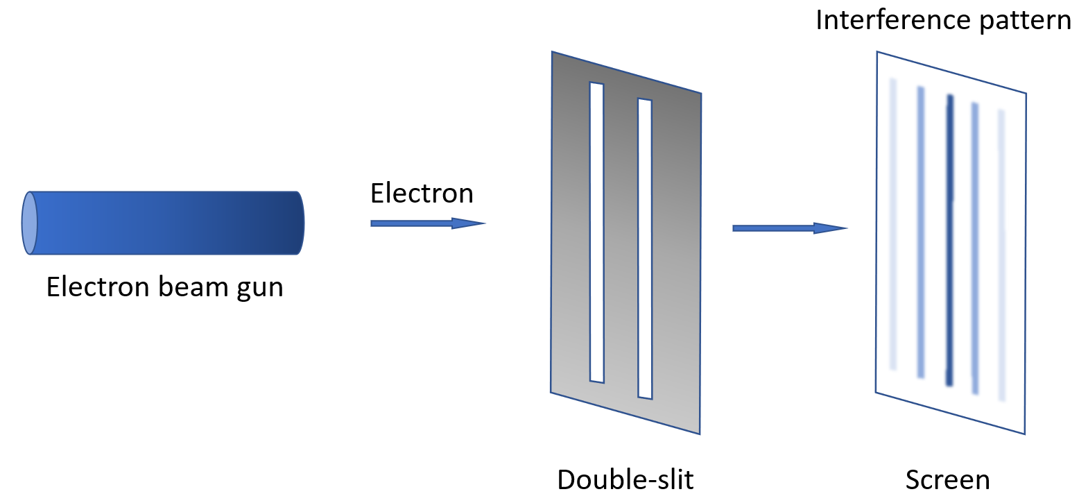
Figure 2: Double-slit experiment

1.2 Background

The beginning. The checkers model was invented by R. Feynman in 1940s [43] and first published in 1965 [12]. In Problem 2.6 there, a function on a lattice of small step $\varepsilon$ was constructed (called kernel; see (2)) and the following task was posed:

If the time interval is very long ($t_{b}-t_{a}\gg\hbar/mc^{2}$) and the average velocity is small [$x_{b}-x_{a}\ll c(t_{b}-t_{a})$], show that the resulting kernel is approximately the same as that for a free particle [given in Eq. (3-3)], except for a factor $\exp[(imc^{2}/\hbar)(t_{b}-t_{a})]$.

Mathematically, this means that the kernel (divided by $2i\varepsilon\exp[(-imc^{2}/\hbar)(t_{b}-t_{a})]$) asymptotically equals free-particle kernel (24) (this is Eq. (3-3) from [12]) in the triple limit when time tends to infinity, whereas the average velocity and the lattice step tend to zero (see Table 1 and Figure 3). Both scaling by the lattice step and tending it to zero were understood, otherwise the mentioned ‘‘exceptional’’ factor would be different (see Example 4). We show that the assertion, although incorrect literally, holds under mild assumptions (see Corollary 5).

Although the Feynman problem might seem self-evident for theoretical physicists, even the first step of a mathematical solution (disproving the assertion as stated) is not found in literature. As usual, the difficulty is to prove the convergence rather than to guess the limit.

propagator	continuum	lattice	context	references
free-particle kernel	(24)	-	quantum mechanics	[12, (3-3)]
spin-$1/2$ retarded propagator	(26),(27)	(2)	relativistic	cf. [23, (13)]
			quantum mechanics	and [12, (2-27)]
spin-$1/2$ Feynman propagator	(34),(35)	(32)	quantum field theory	cf. [2, §9F]

Table 1: Expressions for the propagators of a particle freely moving in $1$ space and $1$ time dimension. The meaning of the norm square of a propagator is the relative probability density to find the particle at a particular point, or alternatively, the charge density at the point.

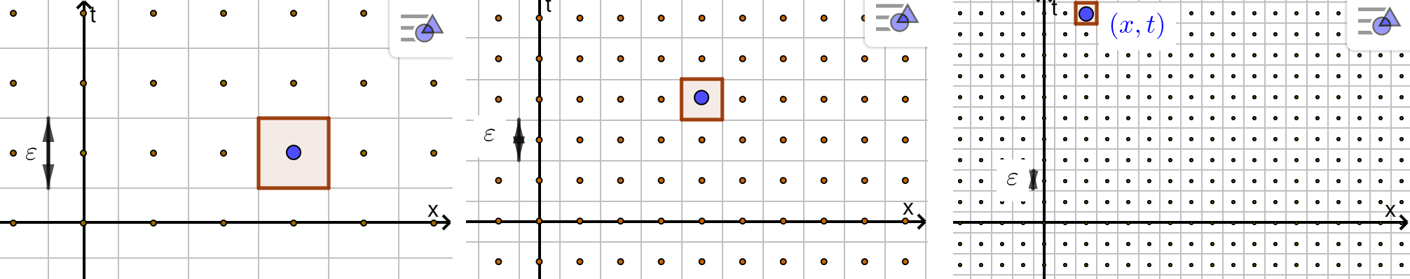
Figure 3: The Feynman triple limit: $t\to+\infty$, $x/t\to 0$, $\varepsilon\to 0$

In 1972 J. Narlikar discovered that the above kernel reproduces the spin-$1/2$ retarded propagator in the different limit when the lattice step tends to zero but time stays fixed [36] (see Table 1, Figures 4 and 1, Corollary 6). In 1984 T.Jacobson–L.Schulman repeated this derivation, applied stationary phase method among other bright ideas, and found the probability of changing the movement direction [23] (cf. Theorem 6). The remarkable works of that period contain no mathematical proofs, but approximate computations without estimating the error.

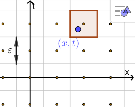
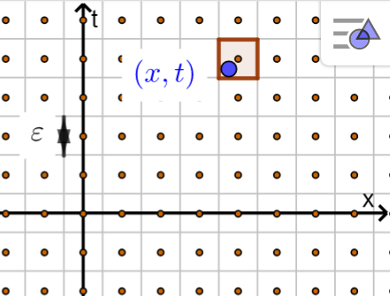
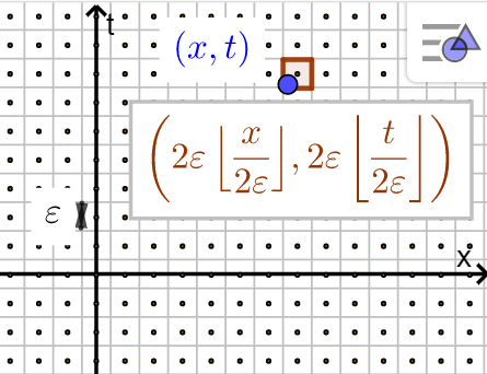
Figure 4: Continuum limit: the point $(x,t)$ stays fixed while the lattice step $\varepsilon$ tends to zero

Ising model. In 1981 H. Gersch noticed that Feynman checkers can be viewed as a $1$-dimensional Ising model with imaginary temperature or edge weights (see §2.2 and [18], [23, §3]). Imaginary values of these quantities are usual in physics (e.g., in quantum field theory or in alternating current networks). Due to the imaginarity, contributions of most configurations cancel each other, which makes the model highly nontrivial in spite of being $1$-dimensional. In particular, the model exhibits a phase transition (see Figures 1 and 5). Surprisingly, the latter seems to have never been reported before. Phase transitions were studied only in more complicated $1$-dimensional Ising models [25, §III], [35], in spite of a known equivalent result, which we are going to discuss now (see Theorem 1(B) and Corollary 3).

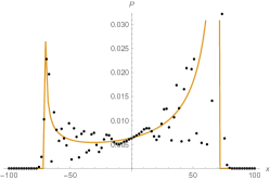
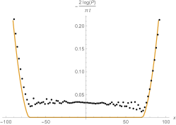
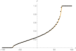
Figure 5: The distribution of the electron position $x$ at time $t=100$ in natural units for the basic model from §2 (left, dots). Its normalized logarithm (middle, dots) and cumulative distribution function (right, dots). Their (weak) scaling limits as $t\to\infty$ (curves). The middle plot is also (minus the imaginary part of) the limiting free energy density in the Ising model. The non-analyticity of the curves reflects a phase transition.

Quantum walks. In 2001 A. Ambainis, E. Bach, A. Nayak, A. Vishwanath, and J. Watrous performed a breakthrough [1]. They studied Feynman checkers under names one-dimensional quantum walk and Hadamard walk; although those cleverly defined models were completely equivalent to Feynman’s simple one. They computed the large-time limit of the model (see Theorem 2). They discovered several striking properties having sharp contrast with both continuum theory and the classical random walks. First, the most probable average electron velocity in the model equals $1/\sqrt{2}$ of the speed of light, and the probability of exceeding this value is very small (see Figures 5 and 1 to the left and Theorem 1(B)). Second, if an absorbing boundary is put immediately to the left of the starting position, then the probability that the electron is absorbed is $2/\pi$. Third, if an additional absorbing boundary is put at location $x>0$, the probability that the electron is absorbed to the left actually increases, approaching $1/\sqrt{2}$ in the limit $x\to+\infty$. Recall that in the classical case both absorption probabilities are $1$. In addition, they found many combinatorial identities and expressed the above kernel through the values of Jacobi polynomials at a particular point (see Remark 3; cf. [48, §2]).

N. Konno studied a biased quantum walk [29, 30], which is still essentially equivalent to Feynman checkers (see Remark 4). He found the distribution of the electron position in the (weak) large-time limit (see Figure 5 and Theorem 1(B)). This result was proved mathematically by G.R. Grimmett–S. Janson–P.F. Scudo [20]. In their seminal paper [47] from 2012, T. Sunada–T. Tate found and proved a large-time asymptotic formula for the distribution (see Theorems 2–4). This was a powerful result but it still could not solve the Feynman problem because the error estimate was not uniform in the lattice step. In 2018 M. Maeda et al. proved a bound for the maximum of the distribution for large time [33, Theorem 2.1].

Quantum walks were generalized to arbitrary graphs and applied to quantum algorithms (see Figure 6 and [17] for an implementation). We refer to the surveys by M.J. Cantero–F.A. Grünbaum–L. Moral–L. Velázquez, N. Konno, J. Kempe, and S.E. Venegas-Andraca [7, 30, 27, 50, 31] for further details in this direction.

Lattice quantum field theories. In a more general context, this is a direction towards creation of Minkowskian lattice quantum field theory, with both space and time being discrete [2]. In 1970s F. Wegner and K. Wilson introduced lattice gauge theory as a computational tool for gauge theory describing all known interactions (except gravity); see [34] for a popular-science introduction. This culminated in determining the proton mass theoretically with error less than $2\%$ in a sense. This theory is Euclidean in the sense that it involves imaginary time. Likewise, an asymptotic formula for the propagator for the (massless) Euclidean lattice Dirac equation [28, Theorem 4.3] played a crucial role in the continuum limit of the Ising model performed by D. Chelkak–S. Smirnov [8]. Similarly, asymptotic formulae for the Minkowskian one (Theorems 2–5) can be useful for missing Minkowskian lattice quantum field theory. Several authors argue that Feynman checkers have the advantage of no fermion doubling inherent in Euclidean lattice theories and avoid the Nielsen–Ninomiya no-go theorem [4, 15].

Several upgrades of Feynman checkers have been discussed. For instance, around 1990s B. Gaveau–L. Schulman and G. Ord added electromagnetic field to the model [16, 38]. That time they achieved neither exact charge conservation nor generalization to non-Abelian gauge fields; this is fixed in Definition 3. Another example is adding mass matrix by P. Jizba [24].

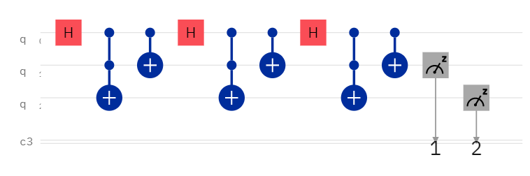
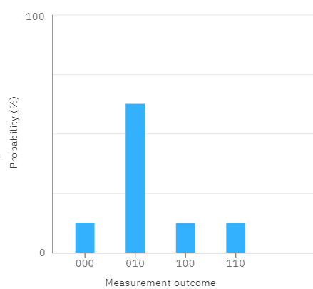
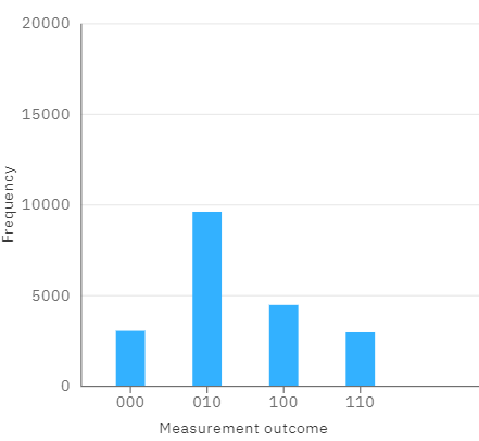
Figure 6: Implementation of the basic model from §2 on a quantum computer using quantum-circuit language (left). The output is a random bit-string coding electron position $x$ at time $t=4$. The strings 000, 010, 100, 110 code $x=4,2,0,-2$ respectively. Distribution of $x$ (middle) and a histogram for quantum computer IBM-Lima (right) [44, §19]. See [17] for details.

It was an old dream to incorporate also checker paths turning backwards in time or forming cycles [43, p. 481–483], [22]; this would mean creation of electron-positron pairs, celebrating a passage from quantum mechanics to quantum field theory. One looked for a combinatorial model reproducing the Feynman propagator rather than the retarded one in the continuum limit (see Table 1). Known constructions (such as hopping expansion) did not lead to the Feynman propagator because of certain lattice artifacts (e.g., the title of [39] is misleading: the Feynman propagator is not discussed there). In the massless case, a noncombinatorial construction of Feynman propagator on the lattice was provided by C. Bender–L. Mead–K. Milton–D. Sharp in [2, §9F] and [3, §IV]. In Definition 6 the desired combinatorial construction is finally given.

Another long-standing open problem is to generalize the model to the $4$-dimensional real world. In his Nobel prize lecture, R. Feynman mentioned his own unsuccessful attempts. There are several recent approaches, e.g., by B. Foster–T. Jacobson from 2017 [15]. Those are not yet as simple and beautiful as the original $2$-dimensional model, as it is written in [15, §7.1] itself.

On physical and mathematical works. The physical literature on the subject is quite extensive [50], and we cannot mention all remarkable works in this brief overview. Surprisingly, in the whole literature we have not found the shouting property of concentration of measure for lattice step tending to zero (see Corollary 7). Many papers are well-written, insomuch that the physical theorems and proofs there could be carelessly taken for mathematical ones (see the end of §12). We are aware of just a few mathematical works on the subject, such as [20, 47, 33].

1.3 Contributions

We solve mathematically a problem by R. Feynman from 1965, which was to prove that his model is consistent with the continuum one, namely, reproduces the usual quantum-mechanical free-particle kernel for large time, small average velocity, and small lattice step (see Corollary 5). We compute large-time and small-lattice-step asymptotic formulae for the lattice propagator, uniform in the model parameters (see Theorems 2 and 5). For the first time we observe and prove concentration of measure in the continuum limit: the average velocity of an electron emitted by a point source is close to the speed of light with high probability (see Corollary 7). The results can be interpreted as asymptotic properties of Young diagrams (see Corollary 2) and Jacobi polynomials (see Remark 3).

All these results are proved mathematically for the first time. For their statements, just Definition 2 is sufficient. In Definitions 3 and 6 we perform a coupling to lattice gauge theory and the second quantization of the model, promoting Feynman checkers to a full-fledged lattice quantum field theory.

1.4 Organization of the paper and further directions

First we give the definitions and precise statements of the results, and in the process provide a zero-knowledge examples for basic concepts of quantum theory. These are precisely those examples that R. Feynman presents first in his own books: Feynman checkers (see §3) is the first specific example in the whole book [12]. The thin-film reflection (see §7) is the first example in [11]; see Figures 10–11 there. Thus we hope that these examples could be enlightening to readers unfamiliar with quantum theory.

We start with the simplest (and rough) particular case of the model and upgrade it step by step in each subsequent section. Before each upgrade, we summarize which physical question does it address, which simplifying assumptions does it resolve or impose additionally, and which experimental or theoretical results does it reproduce. Some upgrades (§§7–9) are just announced to be discussed in a subsequent publication. Our aim is (1+1)-dimensional lattice quantum electrodynamics (‘‘QED’’) but the last step on this way (mentioned in §10) is still undone. Open problems are collected in §11. For easier navigation, we present the upgrades-dependence chart:

Hopefully this is a promising path to making quantum field theory rigorous and algorithmic. An algorithmic quantum field theory would be a one which, given an experimentally observable quantity and a number $\delta>0$, would provide a precise statement of an algorithm predicting a value for the quantity within accuracy $\delta$. (Surely, the predicted value needs not to agree with the experiment for $\delta$ less than accuracy of theory itself.) See Algorithm 1 for a toy example. This would be an extension of constructive quantum field theory (currently far from being algorithmic). Application of quantum theory to computer science is in mainstream now, but the opposite direction could provide benefit as well. (Re)thinking algorithmically is a way to make a subject available to nonspecialists, as it is happening with, say, algebraic topology.

The paper is written in a mathematical level of rigor, in the sense that all the definitions, conventions, and theorems (including corollaries, propositions, lemmas) should be understood literally. Theorems remain true, even if cut out from the text. The proofs of theorems use the statements but not the proofs of the other ones. Most statements are much less technical than the proofs; hence the proofs are kept in a separate section (§12) and long computations are kept in [44]. In the process of the proofs, we give a zero-knowledge introduction to the main tools to study the model: combinatorial identities, the Fourier transform, the method of moments, the stationary phase method. Remarks are informal and usually not used elsewhere (hence skippable). Text outside definitions, theorems, proofs is neither used formally.

2 Basic model (Hadamard walk)

 Question: what is the probability to find an electron in the square $(x,t)$, if it was emitted from $(0,0)$?

Assumptions: no self-interaction, no creation of electron-positron pairs, fixed mass and lattice step, point source; the electron moves in a plane ‘‘drifting uniformly along the $t$-axis’’ or along a line (and then $t$ is time).

Results: double-slit experiment (qualitative explanation), charge conservation, large-time limiting distribution.  

2.1 Definition and examples

We first give an informal definition of the model in the spirit of [11] and then a precise one.

On an infinite checkerboard, a checker moves to the diagonal-neighboring squares, either upwards-right or upwards-left (see Figure 7 to the left). To each path $s$ of the checker, assign a vector ${a}(s)$ as follows (see Figure 7 to the middle). Take a stopwatch that can time the checker as it moves. Initially the stopwatch hand points upwards. While the checker moves straightly, the hand does not rotate, but each time when the checker changes the direction, the hand rotates through $90^{\circ}$ clockwise (independently of the direction the checker turns). The final direction of the hand is the direction of the required vector ${a}(s)$. The length of the vector is set to be $1/2^{(t-1)/2}$, where $t$ is the total number of moves (this is just a normalization). For instance, for the path $s$ in Figure 7 to the top-middle, the vector ${a}(s)=(0,-1/2)$.

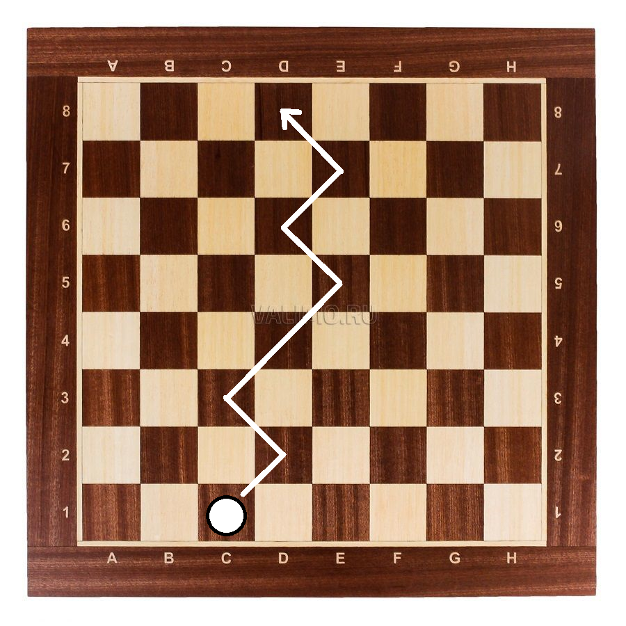
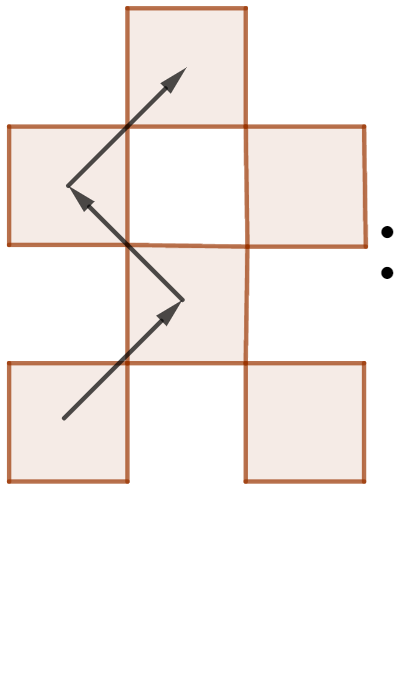
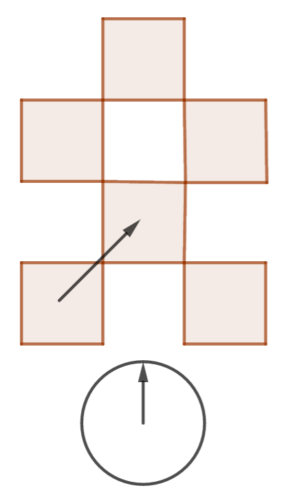
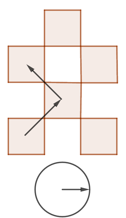
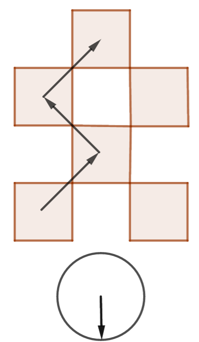
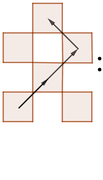
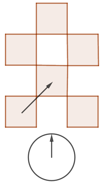
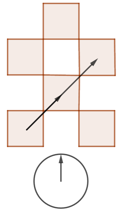
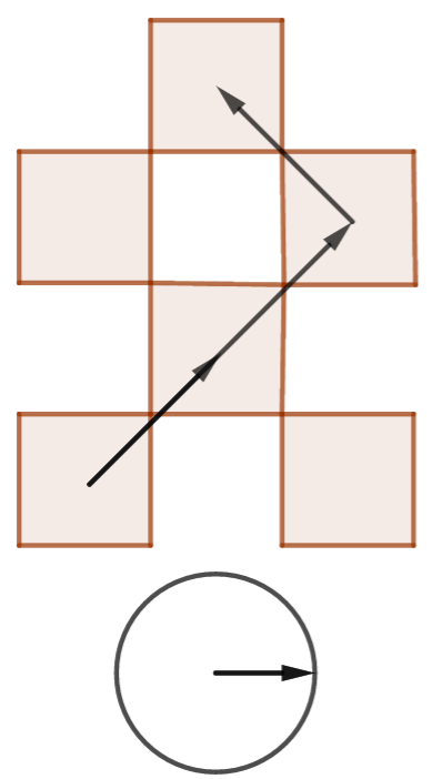
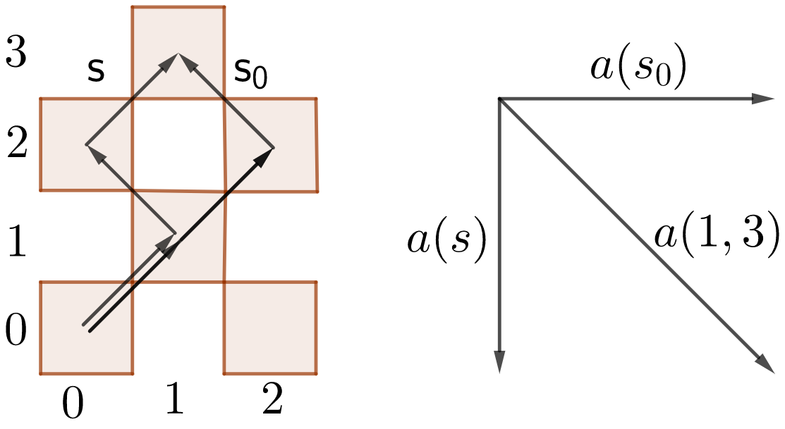
Figure 7: A checker path (left). The vectors assigned to paths (middle) and a square (right).

Denote by ${a}(x,t):=\sum_{s}{a}(s)$ the sum over all the checker paths from the square $(0,0)$ to the square $(x,t)$, starting with the upwards-right move. For instance, ${a}(1,3)=(0,-1/2)+(1/2,0)=(1/2,-1/2)$; see Figure 7 to the right. The length square of the vector ${a}(x,t)$ is called the probability to find an electron in the square $(x,t)$, if it was emitted from $(0,0)$ (see §2.2 for a discussion of the terminology). The vector ${a}(x,t)$ itself is called the arrow [11, Figure 6].

Let us summarize this construction rigorously.

Definition 1.

A checker path is a finite sequence of integer points in the plane such that the vector from each point (except the last one) to the next one equals either $(1,1)$ or $(-1,1)$. A turn is a point of the path (not the first and not the last one) such that the vectors from the point to the next and to the previous ones are orthogonal. The arrow is the complex number

$${a}(x,t):=2^{(1-t)/2}\,i\,\sum_{s}(-i)^{\mathrm{turns}(s)},$$

where the sum over all checker paths $s$ from $(0,0)$ to $(x,t)$ with the first step to $(1,1)$, and $\mathrm{turns}(s)$ is the number of turns in $s$. Hereafter an empty sum is $0$ by definition. Denote

$$P(x,t):=|{a}(x,t)|^{2},\qquad{a_{1}(x,t):=\mathrm{Re}\,{a}(x,t)},\qquad{a_{2}(x,t):=\mathrm{Im}\,{a}(x,t)}.$$

Points (or squares) $(x,t)$ with even and odd $x+t$ are called black and white respectively.

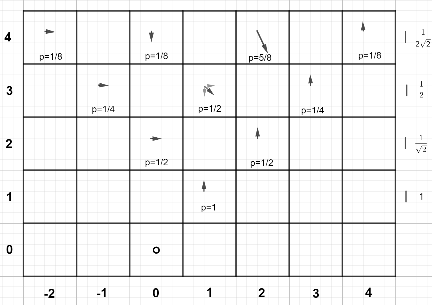
Figure 8: The arrows $a(x,t)$ and the probabilities $P(x,t)$ for small $x,t$ (left); the scale depends on the row. The arrows $10\cdot a(x,t)$ for $t\leq 50$ (right).

$4$	$\frac{1}{2\sqrt{2}}$		$-\frac{i}{2\sqrt{2}}$		$\frac{1-2i}{2\sqrt{2}}$		$\frac{i}{2\sqrt{2}}$
$3$		$\frac{1}{2}$		$\frac{1-i}{2}$		$\frac{i}{2}$
$2$			$\frac{1}{\sqrt{2}}$		$\frac{i}{\sqrt{2}}$
$1$				$i$
	$-2$	$-1$	$0$	$1$	$2$	$3$	$4$

Table 2: The arrows $a(x,t)$ for small $x,t$.

Figure 8 and Table 2 depict the arrows $a(x,t)$ and the probabilities $P(x,t)$ for small $x,t$. Figure 9 depicts the graphs of $P(x,1000)$, $a_{1}(x,1000)$, and $a_{2}(x,1000)$ as functions in an even number $x$. We see that under variation of the final position $x$ at a fixed large time $t$, right after the peak the probability falls to very small although still nonzero values. What is particularly interesting is the unexpected position of the peak, far from $x=1000$. In Figure 1 to the left, the color of a point $(x,t)$ with even $x+t$ depicts the value $P(x,t)$. Notice that the sides of the apparent angle are not the lines $t=\pm x$ but the lines $t=\pm\sqrt{2}x$ (see Theorem 1(A)).

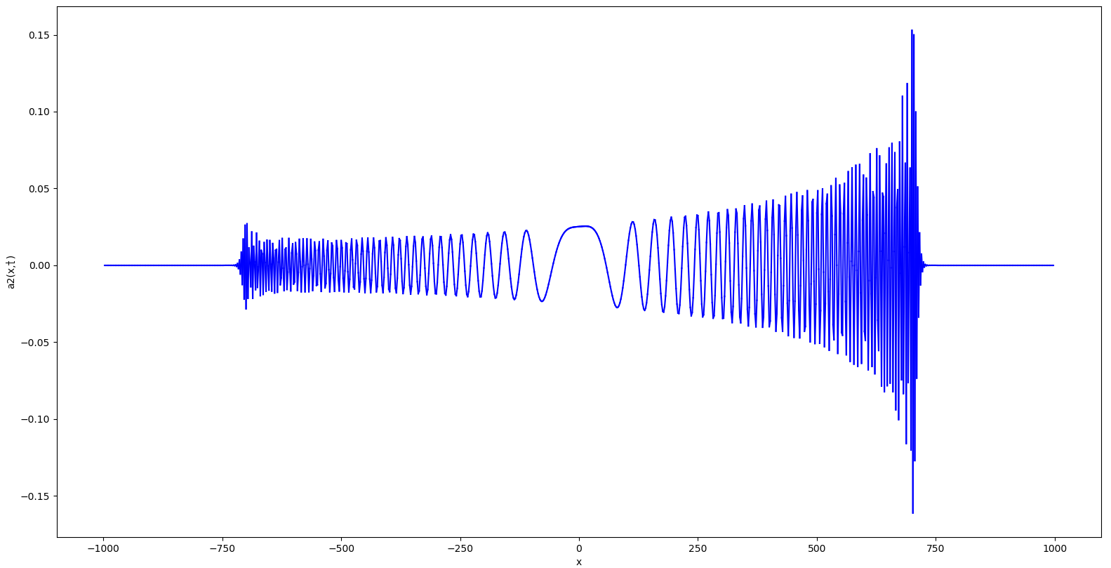
Figure 9: The plots of $P(x,1000),a_{1}(x,1000),a_{2}(x,1000)$

2.2 Physical interpretation

Let us comment on the physical interpretation of the model and ensure that it captures unbelievable behavior of electrons. There are two different interpretations; see Table 3.

object	standard interpretation	spin-chain interpretation
$s$	path	configuration of ‘‘$+$’’ and ‘‘$-$’’ in a row
$\mathrm{turns}(s)$	number of turns	half of the configuration energy
$t$	time	volume
$x$	position	difference between the number of ‘‘$+$’’ and ‘‘$-$’’
$x/t$	average velocity	magnetization
$a(x,t)$	probability amplitude	partition function up to constant
$P(x,t)$	probability	partition function norm squared
$\dfrac{4i}{\pi t}\log a(x,t)$	normalized logarithm of amplitude	free energy density
$\dfrac{i\,a_{2}(x,t)}{a(x,t)}$	conditional probability amplitude of the last move upwards-right	‘‘probability’’ of equal signs at the ends of the spin chain

Table 3: Physical interpretations of Feynman checkers

Standard interpretation. Here the $x$- and $t$-coordinates are interpreted as the electron position and time respectively. Sometimes (e.g., in Example 1) we a bit informally interpret both as position, and assume that the electron performs a ‘‘uniform classical motion’’ along the $t$-axis. We work in the natural system of units, where the speed of light, the Plank and the Boltzmann constants equal $1$. Thus the lines $x=\pm t$ represent motion with the speed of light. Any checker path lies above both lines, i.e. in the light cone, which means agreement with relativity: the speed of electron cannot exceed the speed of light.

To think of $P(x,t)$ as a probability, consider the $t$-coordinate as fixed, and the squares $(-t,t),(-t+2,t),\dots,(t,t)$ as all the possible outcomes of an experiment. For instance, the $t$-th horizontal might be a screen detecting the electron. We shall see that all the numbers $P(x,t)$ on one horizontal sum up to $1$ (Proposition 2), thus indeed can be considered as probabilities. Notice that the probability to find the electron in a set $X\subset\mathbb{Z}$ is $P(X,t):=\sum_{x\in X}P(x,t)=\sum_{x\in X}|a(x,t)|^{2}$ rather than $\left|\sum_{x\in X}a(x,t)\right|^{2}$ (cf. [11, Figure 50]).

In reality, one cannot measure the electron position exactly. A fundamental limitation is the electron reduced Compton wavelength $\lambda=1/m\approx 4\cdot 10^{-13}$ meters, where $m$ is the electron mass. Physically, the basic model approximates the continuum by a lattice of step exactly $\lambda$. But that is still a rough approximation: one needs even smaller step to prevent accumulation of approximation error at larger distances and times. For instance, Figures 1 and 10 to the left show a finite-lattice-step effect (renormalization of speed of light): the average velocity $x/t$ cannot exceed $1/\sqrt{2}$ of the speed of light with high probability. (An explanation in physical terms: lattice regularization cuts off distances smaller than the lattice step, hence small wavelengths, hence large momenta, and hence large velocities.) A more precise model is given in §3: compare the plots in Figure 1.

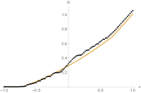
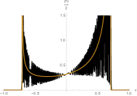
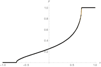
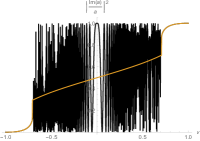
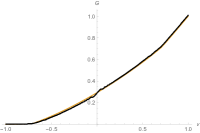
Figure 10: The plots of $\frac{t}{2}P(2\lceil\frac{vt}{2}\rceil,t)$, $F_{t}(v):=\sum\limits_{x\leq vt}P(x,t)$, $\left|\frac{a_{2}(2\lceil{vt}/{2}\rceil,t)}{a(2\lceil{vt}/{2}\rceil,t)}\right|^{2}$, $G_{t}(v):=\sum\limits_{x\leq vt}\frac{2}{t}\left|\frac{a_{2}(x,t)}{a(x,t)}\right|^{2}$ (dark) for $t=100$ (top), $t=1000$ (bottom), and their distributional limits as $t\to\infty$ (light).

As we shall see now, the model qualitatively captures unbelievable behavior of electrons. (For correct quantitative results like exact shape of an interferogram, an upgrade involving a coherent source is required; see §6.)

The probability to find an electron in the square $(x,t)$ subject to absorption in a subset $B\subset\mathbb{Z}^{2}$ is defined analogously to $P(x,t)$, only the summation is over checker paths $s$ that have no common points with $B$ possibly except $(0,0)$ and $(x,t)$. The probability is denoted by $P(x,t\text{ bypass }B)$. Informally, this means an additional outcome of the experiment: the electron has been absorbed and has not reached the  screen. In the following example, we view the two black squares $(\pm 1,1)$ on the horizontal $t=1$ as two slits in a horizontal plate (cf. Figure 2).

Example 1 (Double-slit experiment).

Distinct paths cannot be viewed as ‘‘mutually exclusive’’:

$$P(0,4)\neq P(0,4\text{ bypass }\{(2,2)\})+P(0,4\text{ bypass }\{(0,2)\}).$$

Absorption can increase probabilities at some places: $P(0,4)=1/8<1/4=P(0,4\text{ bypass }\{(2,2)\})$.

The standard interpretation of Feynman checkers is also known as the Hadamard walk, or more generally, the 1-dimensional quantum walk or quantum lattice gas. Those are all equivalent but lead to generalizations in distinct directions [50, 31, 51]. For instance, a unification of the upgrades from §3–7 gives a general inhomogeneous 1-dimensional quantum walk.

The striking properties of quantum walks discussed in §1.2 are stated precisely as follows:

$$\sum_{t=1}^{\infty}P(0,t\text{ bypass }\{x=0\})=\frac{2}{\pi}\leq\sum_{t=1}^{\infty}P(0,t\text{ bypass }\{x=0\}\cup\{x=n\})\to\frac{1}{\sqrt{2}}\text{ as }n\to+\infty.$$

Recently M. Dmitriev [10] has found $\sum_{t=1}^{\infty}P(n,t\text{ bypass }\{x=n\})$ for a few values $n\neq 0$ (see Problem 6). Similar numbers appear in the simple random walk on $\mathbb{Z}^{2}$ [41, Table 2].

Spin-chain interpretation. There is a very different physical interpretation of the same model: a $1$-dimensional Ising model with imaginary temperature and fixed magnetization.

Recall that a configuration in the Ising model is a sequence $\sigma=(\sigma_{1},\dots,\sigma_{t})$ of $\pm 1$ of fixed length. The magnetization and the energy of the configuration are $\sum_{k=1}^{t}\sigma_{k}/t$ and $H(\sigma)=\sum_{k=1}^{t-1}(1-\sigma_{k}\sigma_{k+1})$ respectively. The probability of the configuration is $e^{-\beta H(\sigma)}/Z(\beta)$, where the inverse temperature $\beta=1/T>0$ is a parameter and the partition function $Z(\beta):=\sum_{\sigma}e^{-\beta H(\sigma)}$ is a normalization factor. Additional restrictions on configurations $\sigma$ are usually imposed.

Now, moving the checker along a path $s$, write ‘‘$+$’’ for each upwards-right move, and ‘‘$-$’’ for each upwards-left one; see Figure 11 to the left. The resulting sequence of signs is a configuration in the Ising model, the number of turns in $s$ is one half of the configuration energy, and the ratio of the final $x$- and $t$-coordinates is the magnetization. Thus $a(x,t)=\sum_{s}a(s)$ coincides (up to a factor not depending on $x$) with the partition function for the Ising model at the imaginary inverse temperature $\beta=i\pi/4$ under the fixed magnetization $x/t$:

$$a(x,t)=2^{(1-t)/2}\,i\,\sum_{\begin{subarray}{c}(\sigma_{1},\dots,\sigma_{t})\in\{+1,-1\}^{t}:\\ \sigma_{1}=+1,\quad\sum_{k=1}^{t-1}\sigma_{k}=x\end{subarray}}\exp\left(\frac{i\pi}{4}\sum_{k=1}^{t-1}(\sigma_{k}\sigma_{k+1}-1)\right).$$

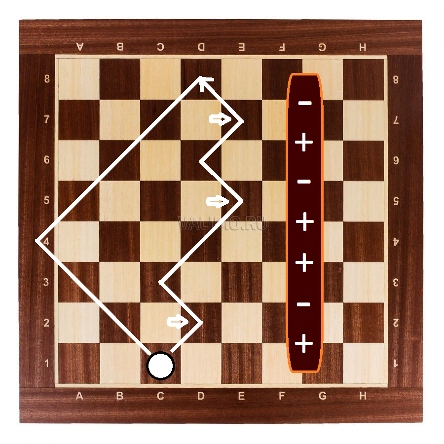
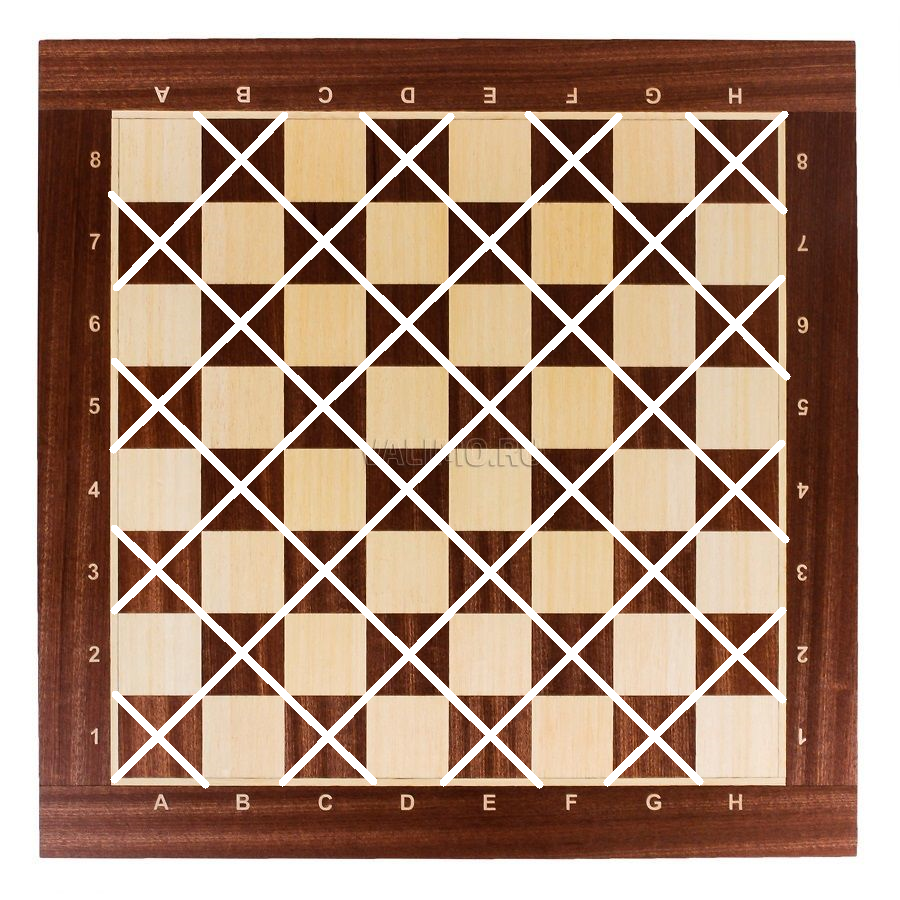
Figure 11: A Young diagram (the arrows point to steps) and the Ising model (left). The auxiliary grid (right).

Notice a crucial difference of the resulting spin-chain interpretation from both the usual Ising model and the above standard interpretation. In the latter two models, the magnetization $x/t$ and the average velocity $x/t$ were random variables; now the magnetization $x/t$ (not to be confused with an external magnetic field) is an external condition. The configuration space in the spin-chain interpretation consists of sequences of ‘‘$+$’’ and ‘‘$-$’’ with fixed numbers of ‘‘$+$’’ and ‘‘$-$’’. Summation over configurations with different $x$ or $t$ would make no sense: e.g., recall that $P(X,t)=\sum_{x\in X}|a(x,t)|^{2}$ rather than $\left|\sum_{x\in X}a(x,t)\right|^{2}$.

Varying the magnetization $x/t$, viewed as an external condition, we observe a phase transition: (the imaginary part of) the limiting free energy density $-\log a(x,t)/\beta t$ is non-analytic when $x/t$ passes through $\pm 1/\sqrt{2}$ (see Figure 5 to the middle and Corollary 3). The phase transition emerges as $t\to\infty$. It is interesting to study other order parameters, for instance, the ‘‘probability’’ $i\,a_{2}(x,t)/a(x,t)$ of equal signs at the endpoints of the spin chain (see Figure 10 and Problems 4–5). These quantities are complex just because the temperature is imaginary.

(A comment for specialists: the phase transition is not related to accumulation of zeroes of the partition function in the plane of complex parameter $\beta$ as in [25, §III] and [35]. In our situation, $\beta=i\pi/4$ is fixed, the real parameter $x/t$ varies, and the partition function $a(x,t)$ has no zeroes at all [37, Theorem 1].)

Young-diagram interpretation. Our results have also a combinatorial interpretation.

The number of steps (or inner corners) in a Young diagram with $w$ columns of heights $x_{1},\dots,x_{w}$ is the number of elements in the set $\{x_{1},\dots,x_{w}\}$; see Figure 11 to the left. Then the value $2^{(h+w-1)/2}\,a_{1}(h-w,h+w)$ is the difference between the number of Young diagrams with an odd and an even number of steps, having exactly $w$ columns and $h$ rows.

Interesting behaviour starts already for $h=w$ (see Proposition 4). For $h=w$ even, the difference vanishes. For $h=w=2n+1$ odd, it is $(-1)^{n}\binom{2n}{n}$. Such $4$-periodicity roughly remains for $h$ close to $w$ [45, Theorem 2]. For fixed half-perimeter $h+w$, the difference slowly oscillates as $h/w$ increases, attains a peak at $h/w\approx 3+2\sqrt{2}$, and then harshly falls to very small values (see Corollary 2 and Theorems 2–4).

Similarly, $2^{(h+w-1)/2}a_{2}(h-w,h+w)$ is the difference between the number of Young diagrams with an even and an odd number of steps, having exactly $w$ columns and less than $h$ rows. The behaviour is similar. The upgrade in §3 is related to Stanley character polynomials [48, §2].

Discussion of the definition. Now compare Definition 1 with the ones in the literature.

The notation ‘‘$a$’’ comes from ‘‘arrow’’ and ‘‘probability amplitude’’; other names are ‘‘wavefunction’’, ‘‘kernel’’, ‘‘the Green function’’, ‘‘propagator’’. More traditional notations are ‘‘$\psi$’’, ‘‘$K$’’, ‘‘$G$’’, ‘‘$\Delta$’’, ‘‘$S$’’ depending on the context. We prefer a neutral one suitable for all contexts.

The factor of $i$ and the minus sign in the definition are irrelevant (and absent in the original definition [12, Problem 2.6]). They come from the ordinary starting direction and rotation direction of the stopwatch hand, and reduce the number of minus signs in what follows.

The normalization factor $2^{(1-t)/2}$ can be explained by analogy to the classical random walk. If the checker were performing just a random walk, choosing one of the two possible directions at each step (after the obligatory first upwards-right move), then $|a(s)|^{2}$ $=2^{1-t}$ would be the probability of a path $s$. This analogy should be taken with a grain of salt: in quantum theory, the ‘‘probability of a path’’ has absolutely no sense (recall Example 1). The reason is that the path is not something one can measure: a measurement of the electron position at one moment strongly affects the motion for all later moments.

Conceptually, one should also fix the direction of the last move of the path $s$ (see [12, bottom of p.35]). Luckily, this is not required in the present paper (and thus is not done), but becomes crucial in further upgrades (see §4 for an explanation).

One could ask where does the definition come from. Following Feynman, we do not try to explain or ‘‘derive’’ it physically. This quantum model cannot be obtained from a classical one by the standard Feynman sum-over-paths approach: there is simply no clear classical analogue of a spin $1/2$ particle (cf. §4) and no true understanding of spin. ‘‘Derivations’’ in [1, 4, 36] appeal to much more complicated notions than the model itself. The true motivation for the model is its simplicity, consistency with basic principles (like probability conservation), and agreement with experiment (which here means the correct continuum limit; see Corollary 6).

2.3 Identities and asymptotic formulae

Let us state several well-known basic properties of the model. The proofs are given in §12.1.

First, the arrow coordinates $a_{1}(x,t)$ and $a_{2}(x,t)$ satisfy the following recurrence relation.

Proposition 1 (Dirac equation).

For each integer $x$ and each positive integer $t$ we have

$$a_{1}(x,t+1) =\frac{1}{\sqrt{2}}a_{2}(x+1,t)+\frac{1}{\sqrt{2}}a_{1}(x+1,t);$$

$$a_{2}(x,t+1) =\frac{1}{\sqrt{2}}a_{2}(x-1,t)-\frac{1}{\sqrt{2}}a_{1}(x-1,t).$$

This mimics the $(1+1)$-dimensional Dirac equation in the Weyl basis [42, (19.4) and (3.31)]

$$\begin{pmatrix}m&\partial/\partial x-\partial/\partial t\\ \partial/\partial x+\partial/\partial t&m\end{pmatrix}\begin{pmatrix}a_{2}(x,t)\\ a_{1}(x,t)\end{pmatrix}=0,$$ (1)

only the derivatives are replaced by finite differences, $m$ is set to $1$, and the normalization factor $1/\sqrt{2}$ is added. For the upgrade in §3, this analogy becomes transparent (see Remark 2). The Weyl basis is not unique, thus there are several forms of equation (1); cf. [23, (1)].

The Dirac equation implies the conservation of probability.

Proposition 2 (Probability/charge conservation).

For each integer $t\geq 1$ we get $\sum\limits_{x\in\mathbb{Z}}\!P(x,t)=1$.

For $a_{1}(x,t)$ and $a_{2}(x,t)$, there is an ‘‘explicit’’ formula (more ones are given in Appendix A).

Proposition 3 (‘‘Explicit’’ formula).

For each integers $|x|<t$ such that $x+t$ is even we have

$$a_{1}(x,t) =2^{(1-t)/2}\sum_{r=0}^{{(t-|x|)/2}}(-1)^{r}\binom{(x+t-2)/2}{r}\binom{(t-x-2)/2}{r},$$

$$a_{2}(x,t) =2^{(1-t)/2}\sum_{r=1}^{{(t-|x|)/2}}(-1)^{r}\binom{(x+t-2)/2}{r}\binom{(t-x-2)/2}{r-1}.$$

The following proposition is a straightforward corollary of the ‘‘explicit’’ formula.

Proposition 4 (Particular values).

For each integer $1\leq k\leq t-1$ the numbers $a_{1}(-t+2k,t)$ and $a_{2}(-t+2k,t)$ are the coefficients at $z^{t-k-1}$ and $z^{t-k}$ in the expansion of the polynomial $2^{(1-t)/2}(1+z)^{t-k-1}(1-z)^{k-1}$. In particular,

$$a_{1}(0,4n+2) =\frac{(-1)^{n}}{2^{(4n+1)/2}}\binom{2n}{n}, a_{1}(0,4n) =0,$$

$$a_{2}(0,4n+2) =0, a_{2}(0,4n) =\frac{(-1)^{n}}{2^{(4n-1)/2}}\binom{2n-1}{n}.$$

In §3.1 we give more identities. The sequences $2^{(t-1)/2}a_{1}(x,t)$ and $2^{(t-1)/2}a_{2}(x,t)$ are present in the on-line encyclopedia of integer sequences [46, A098593 and A104967].

The following remarkable result was observed in [1, §4] (see Figures 5 and 10), stated precisely and derived heuristically in [29, Theorem 1], and proved mathematically in [20, Theorem 1]. See a short exposition of the latter proof in §12.2, and generalizations in §3.2.

Theorem 1 (Large-time limiting distribution; see Figure 10).

$\mathbf{(A)}$ For each $v\in\mathbb{R}$ we have

$$\lim_{t\to\infty}\sum_{x\leq vt}P(x,t)=F(v):=\begin{cases}0,&\mbox{if }v\leq-1/\sqrt{2};\\ \frac{1}{\pi}\arccos\frac{1-2v}{\sqrt{2}(1-v)},&\mbox{if }|v|<1/\sqrt{2};\\ 1,&\mbox{if }v\geq 1/\sqrt{2}.\end{cases}$$

$\mathbf{(B)}$ We have the following convergence in distribution as $t\to\infty$:

$$tP(\lceil vt\rceil,t)\overset{d}{\to}F^{\prime}(v)=\begin{cases}\frac{1}{\pi(1-v)\sqrt{1-2v^{2}}},&\mbox{if }|v|<1/\sqrt{2};\\ 0,&\mbox{if }|v|\geq 1/\sqrt{2}.\end{cases}$$

$\mathbf{(C)}$ For each integer $r\geq 0$ we have $\lim_{t\to\infty}\sum_{x\in\mathbb{Z}}\left(\frac{x}{t}\right)^{r}P(x,t)=\int_{-1}^{1}v^{r}F^{\prime}(v)\,dv.$

Theorem 1(B) demonstrates a phase transition in Feynman checkers, if interpreted as an Ising model at imaginary temperature and fixed magnetization. Recall that then the magnetization $v$ is an external condition (rather than a random variable) and $P(\lceil vt\rceil,t)$ is the norm square of the partition function (rather than a probability). The distributional limit of $tP(\lceil vt\rceil,t)$ is discontinuous at $v=\pm 1/\sqrt{2}$, reflecting a phase transition (cf. Corollary 3).

3 Mass (biased quantum walk)

 Question: what is the probability to find an electron of mass $m$ in the square $(x,t)$, if it was emitted from $(0,0)$?

Assumptions: the mass and the lattice step are now arbitrary.

Results: analytic expressions for the probability for large time or small lattice step, concentration of measure.  

3.1 Identities

Definition 2.

Fix $\varepsilon>0$ and $m\geq 0$ called lattice step and particle mass respectively. Consider the lattice $\varepsilon\mathbb{Z}^{2}=\{\,(x,t):x/\varepsilon,t/\varepsilon\in\mathbb{Z}\,\}$ (see Figure 3). A checker path $s$ is a finite sequence of lattice points such that the vector from each point (except the last one) to the next one equals either $(\varepsilon,\varepsilon)$ or $(-\varepsilon,\varepsilon)$. Denote by $\mathrm{turns}(s)$ the number of points in $s$ (not the first and not the last one) such that the vectors from the point to the next and to the previous ones are orthogonal. For each $(x,t)\in\varepsilon\mathbb{Z}^{2}$, where $t>0$, denote by

$${a}(x,t,m,\varepsilon):=(1+m^{2}\varepsilon^{2})^{(1-t/\varepsilon)/2}\,i\,\sum_{s}(-im\varepsilon)^{\mathrm{turns}(s)}$$ (2)

the sum over all checker paths $s$ on $\varepsilon\mathbb{Z}^{2}$ from $(0,0)$ to $(x,t)$ with the first step to $(\varepsilon,\varepsilon)$. Denote

$$P(x,t,m,\varepsilon):=|{a}(x,t,m,\varepsilon)|^{2},\quad a_{1}(x,t,m,\varepsilon):=\mathrm{Re}\,a(x,t,m,\varepsilon),\quad a_{2}(x,t,m,\varepsilon):=\mathrm{Im}\,a(x,t,m,\varepsilon).$$

Remark 1.

In particular, $P(x,t)=P(x,t,1,1)$ and $a(x,t)=a(x,t,1,1)=a(x\varepsilon,t\varepsilon,1/\varepsilon,\varepsilon)$.

One interprets $P(x,t,m,\varepsilon)$ as the probability to find an electron of mass $m$ in the square $\varepsilon\times\varepsilon$ with the center $(x,t)$, if the electron was emitted from the origin. Notice that the value $m\varepsilon$, hence $P(x,t,m,\varepsilon)$, is dimensionless in the natural units, where $\hbar=c=1$. In Figure 1 to the middle, the color of a point $(x,t)$ depicts the value $P(x,t,1,0.5)$ (if $x+t$ is an integer). Table 4 shows $a(x,t,m,\varepsilon)$ for small $x$ and $t$. Recently I. Novikov elegantly proved that the probability vanishes nowhere inside the light cone: $P(x,t,m,\varepsilon)\neq 0$ for $m>0$, $|x|<t$ and even $(x+t)/\varepsilon$ [37, Theorem 1].

$4\varepsilon$	$\frac{m\varepsilon}{(1+m^{2}\varepsilon^{2})^{3/2}}$		$\frac{(m\varepsilon-m^{3}\varepsilon^{3})-m^{2}\varepsilon^{2}i}{(1+m^{2}\varepsilon^{2})^{3/2}}$		$\frac{m\varepsilon-2m^{2}\varepsilon^{2}i}{(1+m^{2}\varepsilon^{2})^{3/2}}$		$\frac{i}{(1+m^{2}\varepsilon^{2})^{3/2}}$
$3\varepsilon$		$\frac{m\varepsilon}{1+m^{2}\varepsilon^{2}}$		$\frac{m\varepsilon-m^{2}\varepsilon^{2}i}{1+m^{2}\varepsilon^{2}}$		$\frac{i}{(1+m^{2}\varepsilon^{2})}$
$2\varepsilon$			$\frac{m\varepsilon}{\sqrt{1+m^{2}\varepsilon^{2}}}$		$\frac{i}{\sqrt{1+m^{2}\varepsilon^{2}}}$
$\varepsilon$				$i$
	$-2\varepsilon$	$-\varepsilon$	$0$	$\varepsilon$	$2\varepsilon$	$3\varepsilon$	$4\varepsilon$

Table 4: (by I. Novikov [37]) The values $a(x,t,m,\varepsilon)$ for small $x$ and $t$.

Example 2 (Boundary values).

We have $a(t,t,m,\varepsilon)=i(1+m^{2}\varepsilon^{2})^{(1-t/\varepsilon)/2}$ and $a(2\varepsilon-t,t,m,\varepsilon)=m\varepsilon(1+m^{2}\varepsilon^{2})^{(1-t/\varepsilon)/2}$ for each $t\in\varepsilon\mathbb{Z}$, $t>0$, and $a(x,t,m,\varepsilon)=0$ for each $x>t$ or $x\leq-t$.

Example 3 (Massless and heavy particles).

For each $(x,t)\in\varepsilon\mathbb{Z}^{2}$, where $t>0$, we have

$$P(x,t,0,\varepsilon)=\begin{cases}1,&\text{\!for }x=t;\\ 0,&\text{\!for }x\neq t.\end{cases}\quad\text{and}\quad\lim_{m\to\infty}P(x,t,m,\varepsilon)=\begin{cases}1,&\text{\!for }x=0\text{ or }\varepsilon,\text{ and }\frac{x+t}{\varepsilon}\text{ even};\\ 0,&\text{\! otherwise}.\end{cases}$$

Let us list known combinatorial properties of the model [50, 30]; see §12.1 for simple proofs.

Proposition 5 (Dirac equation).

For each $(x,t)\in\varepsilon\mathbb{Z}^{2}$, where $t>0$, we have

$$a_{1}(x,t+\varepsilon,m,\varepsilon) =\frac{1}{\sqrt{1+m^{2}\varepsilon^{2}}}(a_{1}(x+\varepsilon,t,m,\varepsilon)+m\varepsilon\,a_{2}(x+\varepsilon,t,m,\varepsilon)),$$ (3)

$$a_{2}(x,t+\varepsilon,m,\varepsilon) =\frac{1}{\sqrt{1+m^{2}\varepsilon^{2}}}(a_{2}(x-\varepsilon,t,m,\varepsilon)-m\varepsilon\,a_{1}(x-\varepsilon,t,m,\varepsilon)).$$ (4)

Remark 2.

This equation reproduces Dirac equation (1) in the continuum limit $\varepsilon\to 0$: for $C^{2}$ functions $a_{1},a_{2}\colon\mathbb{R}\times(0,+\infty)\to\mathbb{R}$ satisfying (3)–(4) on $\varepsilon\mathbb{Z}^{2}$, the left-hand side of (1) is ${O}_{m}\left(\varepsilon\cdot(\|a_{1}\|_{C^{2}}+\|a_{2}\|_{C^{2}})\right)$.

Proposition 6 (Probability conservation).

For each $t\in\varepsilon\mathbb{Z}$, $t>0$, we get $\sum\limits_{x\in\varepsilon\mathbb{Z}}\!P(x,t,m,\varepsilon)=1$.

Proposition 7 (Klein–Gordon equation).

For each $(x,t)\in\varepsilon\mathbb{Z}^{2}$, where $t>\varepsilon$, we have

$$\sqrt{1+m^{2}\varepsilon^{2}}\,a(x,t+\varepsilon,m,\varepsilon)+\sqrt{1+m^{2}\varepsilon^{2}}\,a(x,t-\varepsilon,m,\varepsilon)-a(x+\varepsilon,t,m,\varepsilon)-a(x-\varepsilon,t,m,\varepsilon)=0.$$

This equation reproduces the Klein–Gordon equation $\tfrac{\partial^{2}a}{\partial t^{2}}-\tfrac{\partial^{2}a}{\partial x^{2}}+m^{2}a=0$ in the limit $\varepsilon\to 0$.

Proposition 8 (Symmetry).

For each $(x,t)\in\varepsilon\mathbb{Z}^{2}$, where $t>0$, we have

$$a_{1}(x,t,m,\varepsilon)=a_{1}(-x,t,m,\varepsilon),\qquad\qquad(t-x)\,a_{2}(x,t,m,\varepsilon)=(t+x-2\varepsilon)\,a_{2}(2\varepsilon-x,t,m,\varepsilon),$$

$$a_{1}(x,t,m,\varepsilon)+m\varepsilon\,a_{2}(x,t,m,\varepsilon)=a_{1}(2\varepsilon-x,t,m,\varepsilon)+m\varepsilon\,a_{2}(2\varepsilon-x,t,m,\varepsilon).$$

Proposition 9 (Huygens’ principle).

For each $x,t,t^{\prime}\in\varepsilon\mathbb{Z}$, where $t>t^{\prime}>0$, we have

$$a_{1}(x,t,m,\varepsilon) =\sum\limits_{x^{\prime}\in\varepsilon\mathbb{Z}}\left[a_{2}(x^{\prime},t^{\prime},m,\varepsilon)a_{1}(x-x^{\prime}+\varepsilon,t-t^{\prime}+\varepsilon,m,\varepsilon)+a_{1}(x^{\prime},t^{\prime},m,\varepsilon)a_{2}(x^{\prime}-x+\varepsilon,t-t^{\prime}+\varepsilon,m,\varepsilon)\right],$$

$$a_{2}(x,t,m,\varepsilon) =\sum\limits_{x^{\prime}\in\varepsilon\mathbb{Z}}\left[a_{2}(x^{\prime},t^{\prime},m,\varepsilon)a_{2}(x-x^{\prime}+\varepsilon,t-t^{\prime}+\varepsilon,m,\varepsilon)-a_{1}(x^{\prime},t^{\prime},m,\varepsilon)a_{1}(x^{\prime}-x+\varepsilon,t-t^{\prime}+\varepsilon,m,\varepsilon)\right].$$

Informally, Huygens’ principle means that each black square $(x^{\prime},t^{\prime})$ on one horizontal acts like an independent point source, with the amplitude and phase determined by $a(x^{\prime},t^{\prime},m,\varepsilon)$.

Proposition 10 (Equal-time recurrence relation).

For each $(x,t)\in\varepsilon\mathbb{Z}^{2}$, where $t>0$, we have

$$(x+\varepsilon)((x-\varepsilon)^{2}-(t-\varepsilon)^{2})a_{1}(x-2\varepsilon,t,m,\varepsilon)+(x-\varepsilon)((x+\varepsilon)^{2}-(t-\varepsilon)^{2})a_{1}(x+2\varepsilon,t,m,\varepsilon)=\\ =2x\left((1+2m^{2}\varepsilon^{2})(x^{2}-\varepsilon^{2})-(t-\varepsilon)^{2}\right)a_{1}(x,t,m,\varepsilon),$$ (5)

$$x((x-2\varepsilon)^{2}-t^{2})a_{2}(x-2\varepsilon,t,m,\varepsilon)+(x-2\varepsilon)(x^{2}-(t-2\varepsilon)^{2})a_{2}(x+2\varepsilon,t,m,\varepsilon)=\\ =2(x-\varepsilon)\left((1+2m^{2}\varepsilon^{2})(x^{2}-2\varepsilon x)-t^{2}+2\varepsilon t\right)a_{2}(x,t,m,\varepsilon).$$

This allows to compute $a_{1}(x,t)$ and $a_{2}(x,t)$ quickly on far horizontals, starting from $x=2\varepsilon-t$ and $x=t$ respectively (see Example 2).

Proposition 11 (‘‘Explicit’’ formula).

For each $(x,t)\in\varepsilon\mathbb{Z}^{2}$ with $|x|<t$ and $(x+t)/\varepsilon$ even,

$$a_{1}(x,t,m,\varepsilon) =(1+m^{2}\varepsilon^{2})^{(1-t/\varepsilon)/2}\sum_{r=0}^{\frac{t-|x|}{2\varepsilon}}(-1)^{r}\binom{(x+t)/2\varepsilon-1}{r}\binom{(t-x)/2\varepsilon-1}{r}(m\varepsilon)^{2r+1},$$ (6)

$$a_{2}(x,t,m,\varepsilon) =(1+m^{2}\varepsilon^{2})^{(1-t/\varepsilon)/2}\sum_{r=1}^{\frac{t-|x|}{2\varepsilon}}(-1)^{r}\binom{(x+t)/2\varepsilon-1}{r}\binom{(t-x)/2\varepsilon-1}{r-1}(m\varepsilon)^{2r}.$$ (7)

Remark 3.

For each $|x|\geq t$ we have $a(x,t,m,\varepsilon)=0$ unless $0<x=t\in\varepsilon\mathbb{Z}$, which gives $a(t,t,m,\varepsilon)=(1+m^{2}\varepsilon^{2})^{(1-t/\varepsilon)/2}i$. Beware that the proposition is not applicable for $|x|\geq t$.

By the definition of Gauss hypergeometric function, we can rewrite the formula as follows:

$$a_{1}(x,t,m,\varepsilon) =m\varepsilon\left({1+m^{2}\varepsilon^{2}}\right)^{(1-t/\varepsilon)/2}\cdot{}_{2}F_{1}\left(1-\frac{x+t}{2\varepsilon},1+\frac{x-t}{2\varepsilon};1;-m^{2}\varepsilon^{2}\right),$$

$$a_{2}(x,t,m,\varepsilon) =m^{2}\varepsilon^{2}\left({1+m^{2}\varepsilon^{2}}\right)^{(1-t/\varepsilon)/2}\cdot{}_{2}F_{1}\left(2-\frac{x+t}{2\varepsilon},1+\frac{x-t}{2\varepsilon};2;-m^{2}\varepsilon^{2}\right)\cdot\left(1-\frac{x+t}{2\varepsilon}\right).$$

This gives a lot of identities. E.g., Gauss contiguous relations connect the values $a(x,t,m,\varepsilon)$ at any $3$ neighboring lattice points; cf. Propositions 5 and 10. In terms of the Jacobi polynomials,

$$a_{1}(x,t,m,\varepsilon) =m\varepsilon(1+m^{2}\varepsilon^{2})^{(x/\varepsilon-1)/2}P_{(x+t)/2\varepsilon-1}^{(0,-x/\varepsilon)}\left(\frac{1-m^{2}\varepsilon^{2}}{1+m^{2}\varepsilon^{2}}\right),$$

$$a_{2}(x,t,m,\varepsilon) =-m^{2}\varepsilon^{2}(1+m^{2}\varepsilon^{2})^{(x/\varepsilon-3)/2}P_{(x+t)/2\varepsilon-2}^{(1,1-x/\varepsilon)}\left(\frac{1-m^{2}\varepsilon^{2}}{1+m^{2}\varepsilon^{2}}\right).$$

There is a similar expression through Kravchuk polynomials (cf. Proposition 4). In terms of Stanley character polynomials (defined in [48, §2]),

$$a_{2}(0,t,m,\varepsilon)=(-1)^{t/2\varepsilon-1}(1+m^{2}\varepsilon^{2})^{(1-t/\varepsilon)/2}\left(\tfrac{t}{2\varepsilon}-1\right)G_{t/2\varepsilon-1}(1;m^{2}\varepsilon^{2}).$$

Proposition 12 (Fourier integral).

Set $\omega_{p}:=\frac{1}{\varepsilon}\arccos(\frac{\cos p\varepsilon}{\sqrt{1+m^{2}\varepsilon^{2}}})$. Then for each $m>0$ and $(x,t)\in\varepsilon\mathbb{Z}^{2}$ such that $t>0$ and $(x+t)/\varepsilon$ is even we have

$$a_{1}(x,t,m,\varepsilon) =\frac{im\varepsilon^{2}}{2\pi}\int_{-\pi/\varepsilon}^{\pi/\varepsilon}\frac{e^{ipx-i\omega_{p}(t-\varepsilon)}\,dp}{\sqrt{m^{2}\varepsilon^{2}+\sin^{2}(p\varepsilon)}},$$

$$a_{2}(x,t,m,\varepsilon) =\frac{\varepsilon}{2\pi}\int_{-\pi/\varepsilon}^{\pi/\varepsilon}\left(1+\frac{\sin(p\varepsilon)}{\sqrt{m^{2}\varepsilon^{2}+\sin^{2}(p\varepsilon)}}\right)e^{ip(x-\varepsilon)-i\omega_{p}(t-\varepsilon)}\,dp.$$

Fourier integral represents a wave emitted by a point source as a superposition of waves of wavelength $2\pi/p$ and frequency $\omega_{p}$.

Proposition 13 (Full space-time Fourier transform).

Denote $\delta_{x\varepsilon}:=1$, if $x=\varepsilon$, and $\delta_{x\varepsilon}:=0$, if $x\neq\varepsilon$. For each $m>0$ and $(x,t)\in\varepsilon\mathbb{Z}^{2}$ such that $t>0$ and $(x+t)/\varepsilon$ is even we get

$$a_{1}(x,t,m,\varepsilon) =\lim_{\delta\to+0}\frac{m\varepsilon^{3}}{4\pi^{2}}\int_{-\pi/\varepsilon}^{\pi/\varepsilon}\int_{-\pi/\varepsilon}^{\pi/\varepsilon}\frac{e^{ipx-i\omega(t-\varepsilon)}\,d\omega dp}{\sqrt{1+m^{2}\varepsilon^{2}}\cos(\omega\varepsilon)-\cos(p\varepsilon)-i\delta},$$

$$a_{2}(x,t,m,\varepsilon) =\lim_{\delta\to+0}\frac{-i\varepsilon^{2}}{4\pi^{2}}\int_{-\pi/\varepsilon}^{\pi/\varepsilon}\int_{-\pi/\varepsilon}^{\pi/\varepsilon}\frac{\sqrt{1+m^{2}\varepsilon^{2}}\sin(\omega\varepsilon)+\sin(p\varepsilon)}{\sqrt{1+m^{2}\varepsilon^{2}}\cos(\omega\varepsilon)-\cos(p\varepsilon)-i\delta}e^{ip(x-\varepsilon)-i\omega(t-\varepsilon)}\,d\omega dp+\delta_{x\varepsilon}\delta_{t\varepsilon}.$$

3.2 Asymptotic formulae

Large-time limit. (See Figure 12) For fixed $m,\varepsilon$, and large time $t$, the function $a(x,t,m,\varepsilon)$

(A)

oscillates in the interval between the (approximate) peaks $x=\pm\frac{t}{\sqrt{1+m^{2}\varepsilon^{2}}}$ (see Theorem 2);

(B)

is approximated by the Airy function around the peaks (see Theorem 3);

(C)

exponentially decays outside the interval bounded by the peaks (see Theorem 4).

We start with discussing regime (A). Let us state our main theorem: an analytic approximation of $a(x,t,m,\varepsilon)$, which is very accurate between the peaks not too close to them (see Figure 12 to the left).

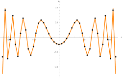
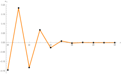
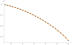
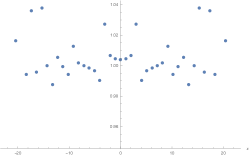
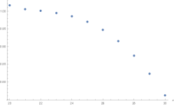
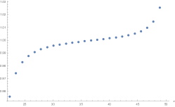
Figure 12: Graphs of $a_{1}(x,50,4,0.5)$ (top, dots), its analytic approximation (top, curves) given by Theorems 2 (left), 3 (middle), and 4 (right), their ratio (bottom). The top-right graph depicts the absolute value of the functions in the logarithmic scale

Theorem 2 (Large-time asymptotic formula between the peaks; see Figure 12 to the left).

For each $\delta>0$ there is $C_{\delta}>0$ such that for each $m,\varepsilon>0$ and each $(x,t)\in\varepsilon\mathbb{Z}^{2}$ satisfying

$$|x|/t<1/\sqrt{1+m^{2}\varepsilon^{2}}-\delta,\qquad\varepsilon\leq 1/m,\qquad t>C_{\delta}/m,$$ (8)

we have

$${a}_{1}\left(x,t+\varepsilon,m,\varepsilon\right) ={\varepsilon}\sqrt{\frac{2m}{\pi}}\left(t^{2}-(1+m^{2}\varepsilon^{2})x^{2}\right)^{-1/4}\sin\theta(x,t,m,\varepsilon)+O_{\delta}\left(\frac{\varepsilon}{m^{1/2}t^{3/2}}\right),$$ (9)

$${a}_{2}\left(x+\varepsilon,t+\varepsilon,m,\varepsilon\right) ={\varepsilon}\sqrt{\frac{2m}{\pi}}\left(t^{2}-(1+m^{2}\varepsilon^{2})x^{2}\right)^{-1/4}\sqrt{\frac{t+x}{t-x}}\cos\theta(x,t,m,\varepsilon)+O_{\delta}\left(\frac{\varepsilon}{m^{1/2}t^{3/2}}\right),$$ (10)

for $$(x+t)/\varepsilon$$ odd and even respectively, where

$$\theta(x,t,m,\varepsilon) :=\frac{t}{\varepsilon}\arcsin\frac{m\varepsilon t}{\sqrt{\left(1+m^{2}\varepsilon^{2}\right)\left(t^{2}-x^{2}\right)}}-\frac{x}{\varepsilon}\arcsin\frac{m\varepsilon x}{\sqrt{t^{2}-x^{2}}}+\frac{\pi}{4}.$$ (11)

Hereafter the notation $f(x,t,m,\varepsilon)=g(x,t,m,\varepsilon)+{O}_{\delta}\left(h(x,t,m,\varepsilon)\right)$ means that there is a constant $C(\delta)$ (depending on $\delta$ but not on $x,t,m,\varepsilon$) such that for each $x,t,m,\varepsilon,\delta$ satisfying the assumptions of the theorem we have $|f(x,t,m,\varepsilon)-g(x,t,m,\varepsilon)|\leq C(\delta)\,h(x,t,m,\varepsilon)$.

The main terms in Theorem 2 were first computed in [1, Theorem 2] in the particular case $m=\varepsilon=1$. The error terms were estimated in [47, Proposition 2.2]; that estimate had the same order in $t$ but was not uniform in $m$ and $\varepsilon$ (and cannot be uniform as it stands, otherwise one would get a contradiction with Corollary 6 as $\varepsilon\to 0$). Getting uniform estimate (9)–(10) has required a refined version of the stationary phase method and additional Steps 3–4 of the proof (see §12.3). Different approaches (Darboux asymptotic formula for Legendre polynomials and Hardy–Littlewood circle method) were used in [6, Theorem 3] and [45, Theorem 2] to get (9) in the particular case $x=0$ and a rougher approximation for $x$ close to $0$ respectively.

Theorem 2 has several interesting corollaries. First, it allows to pass to the large-time distributional limit (see Figure 10). Compared to Theorem 1, it provides convergence in a stronger sense, not immediately accessible by the method of moments and by [47, Theorem 1.1].

Corollary 1 (Large-time limiting distribution).

For each $m>0$ and $\varepsilon\leq 1/m$ we have

$$\sum_{\begin{subarray}{c}x\leq vt\\ x\in\varepsilon\mathbb{Z}\end{subarray}}P(x,t,m,\varepsilon)\rightrightarrows F(v,m,\varepsilon):=\begin{cases}0,&\mbox{if }v\leq-1/\sqrt{1+m^{2}\varepsilon^{2}};\\ \frac{1}{\pi}\arccos\frac{1-(1+m^{2}\varepsilon^{2})v}{\sqrt{1+m^{2}\varepsilon^{2}}(1-v)},&\mbox{if }|v|<1/\sqrt{1+m^{2}\varepsilon^{2}};\\ 1,&\mbox{if }v\geq 1/\sqrt{1+m^{2}\varepsilon^{2}}\end{cases}$$

as $t\to\infty$, $t\in\varepsilon\mathbb{Z}$, uniformly in $v$.

Recall that all our results can be stated in terms of Young diagrams or Jacobi polynomials.

Corollary 2 (Steps of Young diagrams; see Figure 11).

Denote by $n_{+}(h\times w)$ and $n_{-}(h\times w)$ the number of Young diagrams with exactly $h$ rows and $w$ columns, having an even and an odd number of steps (defined in page 11) respectively. Then for almost every $r>1$ we have

$$\limsup_{\begin{subarray}{c}w\to\infty\end{subarray}}\frac{\sqrt{w}}{2^{(r+1)w/2}}\left|n_{+}(\lceil rw\rceil\times w)-n_{-}(\lceil rw\rceil\times w)\right|=\begin{cases}\frac{1}{\sqrt{\pi}}(6r-r^{2}-1)^{-1/4},&\mbox{if }r<3+2\sqrt{2};\\ 0,&\mbox{if }r>3+2\sqrt{2}.\end{cases}$$

For the regimes (B) and (C) around and outside the peaks, we state two theorems by Sunada–Tate without discussing the proofs in detail. (To be precise, the main terms in literature [1, Theorem 2],  [47, Propositions 2.2, 3.1, 4.1] are slightly different from (9), (13), (17); but that difference is within the error term. Practically, the latter three approximations are better by several orders of magnitude.)

Regime (B) around the peaks is described by the Airy function

$$\mathrm{Ai}(\lambda):=\frac{1}{\pi}\int_{0}^{+\infty}\cos\left(\lambda p+\frac{p^{3}}{3}\right)\,dp.$$

Theorem 3 (Large-time asymptotic formula around the peaks; see Figure 12 to the middle).

[47, Proposition 3.1] For each $m,\varepsilon,\Delta>0$ and each sequence $(x_{n},t_{n})\in\varepsilon\mathbb{Z}^{2}$ satisfying

$$|x_{n}/t_{n}-1/\sqrt{1+m^{2}\varepsilon^{2}}|<\Delta\,t_{n}^{-2/3},\qquad t_{n}=n\varepsilon,$$ (12)

we have

$${a}_{1}\left(\pm x_{n},t_{n}+\varepsilon,m,\varepsilon\right) =\left(-1\right)^{\frac{t_{n}-x_{n}-\varepsilon}{2\varepsilon}}m\varepsilon\left(\frac{2}{m^{2}\varepsilon t_{n}}\right)^{1/3}\mathrm{Ai}\left(\Delta(x_{n},t_{n},m,\varepsilon)\right)+O_{m,\varepsilon,\{x_{n}\}}\left(n^{-2/3}\right),$$ (13)

$$a_{2}\left(\pm x_{n}+\varepsilon,t_{n}+\varepsilon,m,\varepsilon\right) =\left(-1\right)^{\frac{t_{n}-x_{n}}{2\varepsilon}}\left(\sqrt{1+m^{2}\varepsilon^{2}}\pm 1\right)\left(\frac{2}{m^{2}\varepsilon t_{n}}\right)^{1/3}\mathrm{Ai}\left(\Delta(x_{n},t_{n},m,\varepsilon)\right)+O_{m,\varepsilon,\{x_{n}\}}\left(n^{-2/3}\right)$$ (14)

for $$(x_{n}+t_{n})/\varepsilon \pm$$ odd and even respectively, where the signs agree and

$$\Delta(x_{n},t_{n},m,\varepsilon) :=\left(\frac{2}{m^{2}\varepsilon t_{n}}\right)^{1/3}\frac{\sqrt{1+m^{2}\varepsilon^{2}}\,x_{n}-t_{n}}{\varepsilon}.$$ (15)

We write $f(x_{n},t_{n},m,\varepsilon)=O_{m,\varepsilon,\{x_{n}\}}\left(g(n)\right)$, if there is a constant $C(m,\varepsilon,\{x_{n}\})$ (depending on $m,\varepsilon$, and the whole sequence $\{x_{n}\}_{n=1}^{\infty}$ but not on $n$) such that for each $n$ we have $|f(x_{n},t_{n},m,\varepsilon)|\leq C(m,\varepsilon,\{x_{n}\})g(n)$.

Recently P. Zakorko has extended (13)–(14) to a larger neighborhood of the peak [52].

Exponential decay outside the peaks was stated without proof in [1, Theorem 1]. A proof appeared only a decade later, when the following asymptotic formula was established.

Theorem 4 (Large-time asymptotic formula outside the peaks; see Figure 12 to the right).

[47, Proposition 4.1] For each $m,\varepsilon,\Delta>0$, $v\in(-1;1)$ and each sequence $(x_{n},t_{n})\in\varepsilon\mathbb{Z}^{2}$ satisfying

$$1/\sqrt{1+m^{2}\varepsilon^{2}}<|v|<1,\qquad|x_{n}-vt_{n}|<\Delta,\qquad t_{n}=n\varepsilon,$$ (16)

we have

$${a}_{1}\left(x_{n},t_{n}+\varepsilon,m,\varepsilon\right) ={\varepsilon}\sqrt{\frac{m}{2\pi t_{n}}}\frac{(-1)^{(t_{n}-|x_{n}|-\varepsilon)/2\varepsilon}}{\left((1+m^{2}\varepsilon^{2})v^{2}-1\right)^{1/4}}\cdot$$

$$\cdot\exp\left(-\frac{t_{n}}{2\varepsilon}H\left(\frac{x_{n}}{t_{n}},m,\varepsilon\right)\right)\left(1+O_{m,\varepsilon,\{x_{n}\}}\left(\frac{1}{n}\right)\right),$$ (17)

$${a}_{2}\left(x_{n}+\varepsilon,t_{n}+\varepsilon,m,\varepsilon\right) ={\varepsilon}\sqrt{\frac{m}{2\pi t_{n}}}\frac{(-1)^{(t_{n}-|x_{n}|)/2\varepsilon}}{\left((1+m^{2}\varepsilon^{2})v^{2}-1\right)^{1/4}}\sqrt{\frac{1+v}{1-v}}\cdot$$

$$\cdot\exp\left(-\frac{t_{n}}{2\varepsilon}H\left(\frac{x_{n}}{t_{n}},m,\varepsilon\right)\right)\left(1+O_{m,\varepsilon,\{x_{n}\}}\left(\frac{1}{n}\right)\right)$$ (18)

for $$(x_{n}+t_{n})/\varepsilon$$ odd and even respectively, where

$$H(v,m,\varepsilon) :=-2\,\mathrm{arcosh}\,\frac{m\varepsilon}{\sqrt{\left(1+m^{2}\varepsilon^{2}\right)\left(1-v^{2}\right)}}+2|v|\,\mathrm{arcosh}\,\frac{m\varepsilon|v|}{\sqrt{1-v^{2}}}.$$ (19)

Function (19) is positive and convex in $v$ in the region $\frac{1}{\sqrt{1+m^{2}\varepsilon^{2}}}<|v|<1$ [47, Theorem 1.4].

Corollary 3 (Limiting free energy density; see Figure 5 to the middle).

For each $m,\varepsilon>0$, $v\in(-1;1)$, and $H(v,m,\varepsilon)$ given by (19) we have

$$\lim_{\begin{subarray}{c}t\to\infty\\ t\in 2\varepsilon\mathbb{Z}\end{subarray}}\frac{1}{t}\log P\left(2\varepsilon\left\lceil\frac{vt}{2\varepsilon}\right\rceil,t,m,\varepsilon\right)=\begin{cases}-H(v,m,\varepsilon)/\varepsilon,&\mbox{if }|v|>1/\sqrt{1+m^{2}\varepsilon^{2}};\\ 0,&\mbox{if }|v|<1/\sqrt{1+m^{2}\varepsilon^{2}}.\end{cases}$$

This means phase transition in the Ising model in a strong sense: the limiting free energy density (with the imaginary part proportional to the left side) is nonanalytic in $v$.

Feynman triple limit. Theorem 2 allows to pass to the limit $(1/t,x/t,\varepsilon)\to 0$ as follows.

Corollary 4 (Simpler and rougher asymptotic formula between the peaks).

Under the assumptions of Theorem 2 we have

$${a}\left(x,t,{m},{\varepsilon}\right)=\varepsilon\sqrt{\frac{2m}{\pi t}}\exp\left(-im\sqrt{t^{2}-x^{2}}+\frac{i\pi}{4}\right)\left(1+{O}_{\delta}\left(\frac{1}{mt}+\frac{|x|}{t}+m^{3}\varepsilon^{2}t\right)\right).$$ (20)

Corollary 5 (Feynman triple limit; see Figure 3).

For each $m\geq 0$ and each sequence $(x_{n},t_{n},\varepsilon_{n})$ such that $(x_{n},t_{n})\in\varepsilon_{n}\mathbb{Z}^{2}$, $(x_{n}+t_{n})/\varepsilon_{n}$ is even, and

$$1/t_{n},\quad x_{n}/t_{n}^{3/4},\quad\varepsilon_{n}t_{n}^{1/2}\quad\to\quad 0\qquad\text{as }\quad n\to\infty,$$ (21)

we have the equivalence

$$\frac{1}{2i\varepsilon_{n}}{a}\left(x_{n},t_{n},{m},{\varepsilon_{n}}\right)\sim\sqrt{\frac{m}{2\pi t_{n}}}\exp\left(-imt_{n}-\frac{i\pi}{4}+\frac{imx_{n}^{2}}{2t_{n}}\right)\qquad\text{ as }\quad n\to\infty.$$ (22)

For equivalence (22), assumptions (21) are essential and sharp, as the next example shows.

Example 4.

Equivalence (22) holds for neither $(x_{n},t_{n},\varepsilon_{n})=(n^{3},n^{4},1/n^{4})$ nor $(0,4n^{2},1/{2n})$ nor $(0,2n\varepsilon,\varepsilon)$, where $\varepsilon=\mathrm{const}<1/m$: the limit of the ratio of the left and the right side equals $e^{im/8}$, $e^{im^{3}/3}$, and does not exist respectively, rather than equals $1$. (The absence of the latter limit confirms that tending $\varepsilon$ to $0$ was understood in the Feynman problem.)

Corollary 5 solves the Feynman problem (and moreover corrects the statement, by revealing the required sharp assumptions). The main difficulty here is that it concerns triple rather than iterated limit. We are not aware of any approach which could solve the problem without proving the whole Theorem 2. E.g., the Darboux asymptotic formula for the Jacobi polynomials (see Remark 3) is suitable for the iterated limit when first $t\to+\infty$, then $\varepsilon\to 0$, giving a (weaker) result already independent on $x$. Neither the Darboux nor Mehler–Heine nor more recent asymptotic formulae [32] are applicable when $1/m\varepsilon$ or $x/\varepsilon$ is unbounded. The same concerns [47, Proposition 2.2] because the error estimate there is not uniform in $m$ and $\varepsilon$. Conversely, the next theorem is suitable for the iterated limit when first $\varepsilon\to 0$, then $x/t\to 0$, then $t\to+\infty$, but not for the triple limit because the error term blows up as $t\to+\infty$.

Continuum limit. The limit $\varepsilon\to 0$ is described by the Bessel functions of the first kind:

$$J_{0}(z) :=\sum_{k=0}^{\infty}(-1)^{k}\frac{(z/2)^{2k}}{(k!)^{2}}, J_{1}(z) :=\sum_{k=0}^{\infty}(-1)^{k}\frac{(z/2)^{2k+1}}{k!(k+1)!}.$$

Theorem 5 (Asymptotic formula in the continuum limit).

For each $m,\varepsilon,\delta>0$ and $(x,t)\in\varepsilon\mathbb{Z}^{2}$ such that $(x+t)/\varepsilon$ even, $t-|x|\geq\delta$, and $\varepsilon<\delta\,e^{-3ms}/16$, where $s:=\sqrt{t^{2}-x^{2}}$, we have

$${a}\left(x,t,{m},{\varepsilon}\right)={m}{\varepsilon}\left(J_{0}(ms)-i\,\frac{t+x}{s}\,J_{1}(ms)+O\left(\frac{\varepsilon}{\delta}\log^{2}\frac{\delta}{\varepsilon}\cdot e^{m^{2}t^{2}}\right)\right).$$

Recall that $f(x,t,{m},{\varepsilon})={O}\left(g(x,t,{m},{\varepsilon})\right)$ means that there is a constant $C$ (not depending on $x,t,{m},{\varepsilon}$) such that for each $x,t,{m},{\varepsilon}$ satisfying the assumptions of the theorem we have $|f(x,t,{m},{\varepsilon})|\leq C\,g(x,t,{m},{\varepsilon})$.

The main term in Theorem 5 was computed in [36, §1]. Numerical experiment shows that the error term decreases faster than asserted (see Table 5 computed in [44, §14]).

In the next corollary, we approximate a fixed point $(x,t)$ in the plane by the lattice point $\left(2\varepsilon\!\left\lceil\frac{x}{2\varepsilon}\right\rceil,2\varepsilon\!\left\lceil\frac{t}{2\varepsilon}\right\rceil\right)$ (see Figure 4). The factors of $2$ make the latter accessible for the checker.

Corollary 6 (Uniform continuum limit; see Figure 4).

For each fixed $m\geq 0$ we have

$$\frac{1}{2\varepsilon}\,{a}\left(2\varepsilon\!\left\lceil\frac{x}{2\varepsilon}\right\rceil,2\varepsilon\!\left\lceil\frac{t}{2\varepsilon}\right\rceil,{m},{\varepsilon}\right)\rightrightarrows\frac{m}{2}\,J_{0}(m\sqrt{t^{2}-x^{2}})-i\,\frac{m}{2}\sqrt{\frac{t+x}{t-x}}\,J_{1}(m\sqrt{t^{2}-x^{2}})$$ (23)

as $\varepsilon\to 0$ uniformly on compact subsets of the angle $|x|<t$.

The proof of pointwise convergence is simpler and is presented in Appendix B.

Corollary 7 (Concentration of measure).

For each $t,m,\delta>0$ we have

$$\sum_{x\in\varepsilon\mathbb{Z}\,:\,0\leq t-|x|\leq\delta}P(x,t,m,\varepsilon)\to 1\qquad\text{as }\quad\varepsilon\to 0\quad\text{ so that }\quad\frac{t}{2\varepsilon}\in\mathbb{Z}.$$

This result, although expected, is not found in literature. An elementary proof is given in §12.6. We remark a sharp contrast between the continuum and the large-time limit here: by Corollary 1, there is no concentration of measure as $t\to\infty$ for fixed $\varepsilon$.

$\varepsilon$	$5\varepsilon\log_{10}^{2}(5\varepsilon)$	$\max\limits_{x\in(-0.8,0.8)\cap 2\varepsilon\mathbb{Z}}\left|\frac{1}{2\varepsilon}a(x,1,10,\varepsilon)-G^{R}_{11}(x,1)-iG^{R}_{12}(x,1)\right|$
0.02	0.1	1.1
0.002	0.04	0.06
0.0002	0.009	0.006

Table 5: Approximation of spin-$1/2$ retarded propagator (26) by Feynman checkers ($m=10$, $\delta=0.2$, $t=1$)

3.3 Physical interpretation

Let us discuss the meaning of the Feynman triple limit and the continuum limit. In this subsection we omit some technical definitions not used in the sequel.

The right side of (22) is up to the factor $e^{-imt_{n}}$ the free-particle kernel

$$K(x,t)=\sqrt{\frac{m}{2\pi t}}\exp\left(\frac{imx^{2}}{2t}-\frac{i\pi}{4}\right),$$ (24)

describing the motion of a non-relativistic particle emitted from the origin along a line.

Limit (23) reproduces the spin-$1/2$ retarded propagator describing motion of an electron along a line. More precisely, the spin-$1/2$ retarded propagator, or the retarded Green function for Dirac equation (1) is a matrix-valued tempered distribution $G^{R}(x,t)=(G^{R}_{kl}(x,t))$ on $\mathbb{R}^{2}$ vanishing for $t<|x|$ and satisfying

$$\begin{pmatrix}m&\partial/\partial x-\partial/\partial t\\ \partial/\partial x+\partial/\partial t&m\end{pmatrix}\begin{pmatrix}G^{R}_{11}(x,t)&G^{R}_{12}(x,t)\\ G^{R}_{21}(x,t)&G^{R}_{22}(x,t)\end{pmatrix}=\delta(x)\delta(t)\begin{pmatrix}1&0\\ 0&1\end{pmatrix},$$ (25)

where $\delta(x)$ is the Dirac delta function. The propagator is given by (cf. [23, (13)], [42, (3.117)])

$$G^{R}(x,t)=\frac{m}{2}\,\begin{pmatrix}J_{0}(m\sqrt{t^{2}-x^{2}})&-\sqrt{\frac{t+x}{t-x}}\,J_{1}(m\sqrt{t^{2}-x^{2}})\\ \sqrt{\frac{t-x}{t+x}}\,J_{1}(m\sqrt{t^{2}-x^{2}})&J_{0}(m\sqrt{t^{2}-x^{2}})\end{pmatrix}\qquad\text{for }|x|<t.$$ (26)

In addition, $G^{R}(x,t)$ involves a generalized function supported on the lines $t=\pm x$, not observed in the limit (23) and not specified here. A more common expression is (cf. Proposition 13)

$$G^{R}(x,t)=\frac{1}{4\pi^{2}}\int_{-\infty}^{+\infty}\int_{-\infty}^{+\infty}\lim_{\delta\to+0}\begin{pmatrix}m&-ip-i\omega\\ -ip+i\omega&m\end{pmatrix}\frac{e^{ipx-i\omega t}\,dpd\omega}{m^{2}+p^{2}-(\omega+i\delta)^{2}},$$ (27)

where the limit is taken in the weak topology of matrix-valued tempered distributions and the integral is understood as the Fourier transform of tempered distributions (cf. [14, (6.47)]).

The propagator ‘‘square’’ $G^{R}_{11}(x,t)^{2}+G^{R}_{12}(x,t)^{2}$ is ill-defined (because of the square of the Dirac delta-function supported on the lines $t=\pm x$ involved). Thus the propagator lacks probabilistic interpretation, and global charge conservation (Proposition 6) has no continuum analogue. For instance, $\int_{(-t,t)}(G^{R}_{11}(x,t)^{2}+G^{R}_{12}(x,t)^{2})\,dx\approx m^{2}t/2\neq\mathrm{const}$ paradoxically. A physical explanation: the line $t=x$ carries infinite charge flowing inside the angle $|x|<t$. One can interpret the propagator ‘‘square’’ for $|x|\neq t$ as a relative probability density or charge density (see Figure 1 to the right). In the spin-chain interpretation, the propagator is the limit of the partition function for one-dimensional Ising model at the inverse temperature $\beta=i\pi/4-\log(m\varepsilon)/2$. Those are essentially the values of $\beta$ for which phase transition is possible [35].

The normalization factor $1/2\varepsilon$ before ‘‘${a}$’’ in (23) can be explained as division by the length associated to one black lattice point on a horizontal line. On a deeper level, it comes from the normalization of $G^{R}(x,t)$ arising from (25).

Theorem 5 is a toy result in algorithmic quantum field theory: it determines the lattice step to compute the propagator with given accuracy. So far this is not a big deal, because the propagator has a known analytic expression and is not really experimentally-measurable; neither the efficiency of the algorithm is taken into account. But that is a first step.

Algorithm 1 (Approximation algorithm for spin-$1/2$ retarded propagator (26)).

Input: mass $m>0$, coordinates $|x|<t$, accuracy level $\Delta$.

Output: an approximate value $G_{kl}$ of $G_{kl}^{R}(x,t)$ within distance $\Delta$ from the true value (26).

Algorithm: compute $G_{kl}=\tfrac{(-1)^{(k-1)l}}{2\varepsilon}\,{a}_{(k+l)\!\!\mod 2+1}\left(2\varepsilon\!\left\lceil\tfrac{(-1)^{(k-1)l}x}{2\varepsilon}\right\rceil,2\varepsilon\!\left\lceil\tfrac{t}{2\varepsilon}\right\rceil,{m},{\varepsilon}\right)$ by (2) for

$$\varepsilon=(t-|x|)\min\left\{\frac{1}{16\,e^{3mt}},\left(\frac{\Delta}{9C\,m\,e^{m^{2}t^{2}}}\right)^{3}\right\},\qquad\text{where }\quad C=100.$$

Here we used an explicit estimate for the constant $C$ understood in the big-O notation in Theorem 5; it is easily extracted from the proof. The theorem and the estimate remain true, if ${a}\left(x,t,{m},{\varepsilon}\right)$ with $(x,t)\in\varepsilon\mathbb{Z}^{2}$ is replaced by ${a}\left(2\varepsilon\!\left\lceil\tfrac{x}{2\varepsilon}\right\rceil,2\varepsilon\!\left\lceil\tfrac{t}{2\varepsilon}\right\rceil,{m},{\varepsilon}\right)$ with arbitrary $(x,t)\in\mathbb{R}^{2}$.

Remark 4.

A general (homogeneous) one-dimensional quantum walk essentially reduces to the upgrade studied in this section. Namely, consider the equation

$$\psi_{1}(x,t+1) =\hphantom{-}a\,\psi_{1}(x+1,t)+b\,\psi_{2}(x+1,t),$$

$$\psi_{2}(x,t+1) =-\bar{b}\,\psi_{1}(x-1,t)+\bar{a}\,\psi_{2}(x-1,t);$$

where $a,b\in\mathbb{C}-\{0\}$ and $|a|^{2}+|b|^{2}=1$, with the initial condition $\psi_{1}(x,0)=\psi_{2}(x,0)=0$ for each $x\neq 0$ [47, §1]. By direct checking using (3)–(4) one finds the solution:

$$\psi_{1}(x,t) =\left(\frac{a}{|a|}\right)^{-x}\left(\frac{|a|b}{a|b|}\,a_{1}\left(x+1,t+1,\left|\frac{b}{a}\right|,1\right)\psi_{2}(0,0)+a_{2}\left(1-x,t+1,\left|\frac{b}{a}\right|,1\right)\psi_{1}(0,0)\right),$$

$$\psi_{2}(x,t) =\left(\frac{a}{|a|}\right)^{-x}\left(a_{2}\left(x+1,t+1,\left|\frac{b}{a}\right|,1\right)\psi_{2}(0,0)-\frac{a|b|}{|a|b}\,a_{1}\left(1-x,t+1,\left|\frac{b}{a}\right|,1\right)\psi_{1}(0,0)\right).$$

4 Spin

 Question: what is the probability to find a right electron at $(x,t)$, if a right electron was emitted from $(0,0)$?

Assumptions: electron chirality is now taken into account.

Results: the probability of chirality flip.  

A feature of the model is that the electron spin emerges naturally rather than is added artificially.

It goes almost without saying to view the electron as being in one of the two states depending on the last-move direction: right-moving or left-moving (or just ‘right’ or ‘left’ for brevity).

The probability to find a right electron in the square $(x,t)$, if a right electron was emitted from the square $(0,0)$, is the length square of the vector $\sum_{s}{a}(s)$, where the sum is over only those paths from $(0,0)$ to $(x,t)$, which both start and finish with an upwards-right move. The probability to find a left electron is defined analogously, only the sum is taken over paths which start with an upwards-right move but finish with an upwards-left move. Clearly, these probabilities equal $a_{2}(x,t)^{2}$ and $a_{1}(x,t)^{2}$ respectively, because the last move is directed upwards-right if and only if the number of turns is even.

These right and left electrons are exactly the $(1+1)$-dimensional analogue of chirality states for a spin $1/2$ particle [42, §19.1]. Indeed, it is known that the components $a_{2}(x,t)$ and $a_{1}(x,t)$ in Dirac equation in the Weyl basis (1) are interpreted as wave functions of right- and left-handed particles respectively. The relation to the movement direction becomes transparent for $m=0$: then a general solution of (1) is $(a_{2}(x,t),a_{1}(x,t))=(a_{2}(x-t,0),a_{1}(x+t,0))$; thus the maxima of $a_{2}(x,t)$ and $a_{1}(x,t)$ (if any) move to the right and to the left respectively as $t$ increases. Beware that in $3$ or more dimensions, spin is not the movement direction and cannot be explained in nonquantum terms.

This gives a more conceptual interpretation of the model: an experiment outcome is a pair (final $x$-coordinate, last-move direction), whereas the final $t$-coordinate is fixed. The probabilities to find a right/left electron are the fundamental ones. In further upgrades, $a_{1}(x,t)$ and $a_{2}(x,t)$ become complex numbers and $P(x,t)$ should be defined as $|{a}_{1}(x,t)|^{2}+|{a}_{2}(x,t)|^{2}$ rather than by the above formula $P(x,t)=|{a}(x,t)|^{2}=|{a}_{1}(x,t)+i{a}_{2}(x,t)|^{2}$, being a coincidence.

Theorem 6 (Probability of chirality flip).

For integer $t>0$ we get $\sum\limits_{x\in\mathbb{Z}}a_{1}(x,t)^{2}=\frac{1}{2\sqrt{2}}+{O}\left(\frac{1}{\sqrt{t}}\right).$

See Figure 13 for an illustration and comparison with the upgrade from §5. The physical interpretation of the theorem is limited: in continuum theory, the probability of chirality flip (for an electron emitted by a point source) is ill-defined similarly to the propagator ‘‘square’’ (see §3.3). A related more reasonable quantity is studied in [23, p. 381] (cf. Problem 5). Recently I. Bogdanov has generalized the theorem to an arbitrary mass and lattice step (see Definition 2): if $0\leq m\varepsilon\leq 1$ then $\lim_{t\to+\infty,t\in\varepsilon\mathbb{Z}}\sum_{x\in\varepsilon\mathbb{Z}}a_{1}(x,t,m,\varepsilon)^{2}=\frac{m\varepsilon}{2\sqrt{1+m^{2}\varepsilon^{2}}}$ [6, Theorem 2]. This has confirmed a conjecture by I. Gaidai-Turlov–T. Kovalev–A. Lvov.

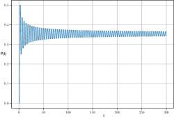
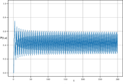
Figure 13: The graphs of the probabilities $P(t)=\sum_{x\in\mathbb{Z}}a_{1}(x,t)^{2}$ and $P(t,u)=\sum_{x\in\mathbb{Z}}a_{1}(x,t,u)^{2}$ of chirality flip with electromagnetic field off and on respectively

5 External field (inhomogeneous quantum walk)

 Question: what is the probability to find an electron at $(x,t)$, if it moves in a given electromagnetic field $u$?

Assumptions: the electromagnetic field vanishes outside the $xt$-plane; it is not affected by the electron.

Results: ‘‘spin precession’’ in a magnetic field (qualitative explanation), charge conservation.  

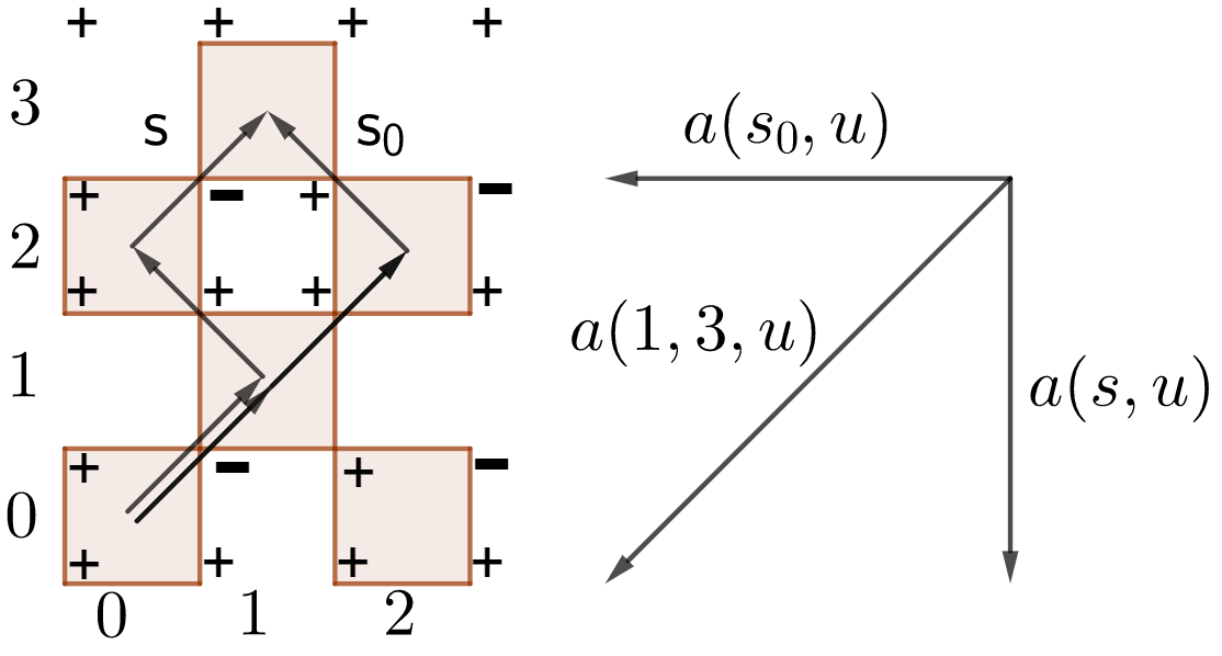
Figure 14: Paths in a field

Another feature of the model is that external electromagnetic field emerges naturally rather than is added artificially. We start with an informal definition, then give a precise one, and finally show exact charge conservation.

In the basic model, the stopwatch hand did not rotate while the checker moved straightly. It goes without saying to modify the model, rotating the hand uniformly during the motion. This does not change the model essentially: since all the paths from the initial to the final position have the same length, their vectors are rotated through the same angle, not affecting probabilities. A more interesting modification is when the current rotation angle depends on the checker position. This is exactly what electromagnetic field does. In what follows, the rotation angle assumes only the two values $0^{\circ}$ and $180^{\circ}$ for simplicity, meaning just multiplication by $\pm 1$.

Thus an electromagnetic field is viewed as a fixed assignment $u$ of numbers $+1$ and $-1$ to all the vertices of the squares. For instance, in Figure 14, the field equals $-1$ at the top-right vertex of each square $(x,t)$ with both $x$ and $t$ even. Modify the definition of the vector ${a}(s)$ by reversing the direction each time when the checker passes through a vertex with the field $-1$. Denote by ${a}(s,u)$ the resulting vector. Define ${a}(x,t,u)$ and $P(x,t,u)$ analogously to ${a}(x,t)$ and $P(x,t)$ replacing ${a}(s)$ by ${a}(s,u)$ in the definition. For instance, if $u=+1$ identically, then $P(x,t,u)=P(x,t)$.

Let us slightly rephrase this construction, making the relation to lattice gauge theory more transparent. We introduce an auxiliary grid with the vertices at the centers of black squares (see Figure 11 to the right). It is the graph where the checker actually moves.

Definition 3.

An auxiliary edge is a segment joining nearest-neighbor integer points with even sum of coordinates. Let $u$ be a map from the set of all auxiliary edges to $\{+1,-1\}$. Denote by

$${a}(x,t,u):=2^{(1-t)/2}\,i\,\sum_{s}(-i)^{\mathrm{turns}(s)}u(s_{0}s_{1})u(s_{1}s_{2})\dots u(s_{t-1}s_{t})$$

the sum over all checker paths $s=(s_{0},s_{1},\dots,s_{t})$ with $s_{0}=(0,0)$, $s_{1}=(1,1)$, and $s_{t}=(x,t)$. Set $P(x,t,u):=|{a}(x,t,u)|^{2}$. Define $a_{1}(x,t,u)$ and $a_{2}(x,t,u)$ analogously to $a(x,t,u)$, only add the condition $s_{t-1}=(x+1,t-1)$ and $s_{t-1}=(x-1,t-1)$ respectively. For half-integers $x,t$ denote by $u(x,t)$ the value of $u$ on the auxiliary edge with the midpoint $(x,t)$.

Remark 5.

Here the field $u$ is a fixed external classical field not affected by the electron.

This definition is analogous to one of the first constructions of gauge theory by Weyl–Fock–London, and gives a coupling of Feynman checkers to the Wegner–Wilson $\mathbb{Z}/2\mathbb{Z}$ lattice gauge theory. In particular, it reproduces the correct spin $1$ for the electromagnetic field: a function defined on the set of edges is a discrete analogue of a vector field, i.e., a spin $1$ field. Although this way of coupling is classical, it has never been explicitly applied to Feynman checkers (cf. [16, p. 36]), and is very different from both the approach of [38] and Feynman-diagram intuition [11].

For instance, the field $u$ in Figure 14 has form $u(s_{1}s_{2})=\exp\left(-i\int_{s_{1}}^{s_{2}}(A_{0}\,dt+A_{1}\,dx)\right)$ for each auxiliary edge $s_{1}s_{2}$, where $(A_{0},A_{1}):=(\pi/2)(x+1/2,x+1/2)$ is the vector-potential of a constant homogeneous electromagnetic field.

For an arbitrary gauge group, $a_{1}(x,t,u)$ and $a_{2}(x,t,u)$ are defined analogously, only $u$ becomes a map from the set of auxiliary edges to a matrix group, e.g., $U(1)$ or $SU(n)$. Then $P(x,t,u):=\sum_{k}\left(|(a_{1}(x,t,u))_{k1}|^{2}+|(a_{2}(x,t,u))_{k1}|^{2}\right)$, where $(a_{j})_{kl}$ are the entries of a matrix $a_{j}$.

Example 5 (‘‘Spin precession’’ in a magnetic field).

Let $u(x+1/2,t+1/2)=-1$, if $x$ and $t$ are even, and $u(x+1/2,t+1/2)=+1$ otherwise (‘‘constant homogeneous field’’; see Figure 14). Then the probability $P(t,u):=\sum_{x\in\mathbb{Z}}a_{1}(x,t,u)^{2}$ of detecting a left electron (see §4) is plotted in Figure 13 to the right. It apparently tends to a ‘‘periodic regime’’ as $t\to\infty$ (see Problem 11).

The following propositions are proved analogously to Propositions 5–6, only a factor of $u(x\pm\tfrac{1}{2},t+\tfrac{1}{2})$ is added due to the last step of the path passing through the vertex $(x\pm\tfrac{1}{2},t+\tfrac{1}{2})$.

Proposition 14 (Dirac equation in electromagnetic field).

For each integers $x$ and $t\geq 1$,

$$a_{1}(x,t+1,u) =\frac{1}{\sqrt{2}}u\left(x+\frac{1}{2},t+\frac{1}{2}\right)(a_{1}(x+1,t,u)+a_{2}(x+1,t,u)),$$

$$a_{2}(x,t+1,u) =\frac{1}{\sqrt{2}}u\left(x-\frac{1}{2},t+\frac{1}{2}\right)({a_{2}(x-1,t,u)}-a_{1}(x-1,t,u)).$$

Proposition 15 (Probability/charge conservation).

For each integer $t\geq 1$, $\sum\limits_{x\in\mathbb{Z}}P(x,t,u)=1$.

Recently F. Ozhegov has found analogues of the ‘‘explicit’’ formula (Proposition 18) and the continuum limit (Corollary 6) for the ‘‘homogeneous field’’ in Example 5 [40, Theorems 3–4].

6 Source

 Question: what is the probability to find an electron at $(x,t)$, if it was emitted by a source of wavelength $\lambda$?

Assumptions: the source is now realistic.

Results: wave propagation, dispersion relation.  

A realistic source produces a wave rather than electrons localized at $x=0$ (as in the basic model). This means solving Dirac equation (3)–(4) with (quasi-)periodic initial conditions.

To state the result, it is convenient to rewrite Dirac equation (3)–(4) using the notation

$$\tilde{a}_{1}(x,t)=a_{1}(x,t+\varepsilon,m,\varepsilon),\qquad\tilde{a}_{2}(x,t)=a_{2}(x+\varepsilon,t+\varepsilon,m,\varepsilon),$$

so that it gets form

$$\tilde{a}_{1}(x,t) =\frac{1}{\sqrt{1+m^{2}\varepsilon^{2}}}(\tilde{a}_{1}(x+\varepsilon,t-\varepsilon)+m\varepsilon\,\tilde{a}_{2}(x,t-\varepsilon)),$$ (28)

$$\tilde{a}_{2}(x,t) =\frac{1}{\sqrt{1+m^{2}\varepsilon^{2}}}(\tilde{a}_{2}(x-\varepsilon,t-\varepsilon)-m\varepsilon\,\tilde{a}_{1}(x,t-\varepsilon)).$$ (29)

The following proposition is proved by direct checking (available in [44, §12]).

Proposition 16 (Wave propagation, dispersion relation).

Equations (28)–(29) with the initial condition

$$\tilde{a}_{1}(x,0) =\tilde{a}_{1}(0,0)e^{2\pi ix/\lambda},$$

$$\tilde{a}_{2}(x,0) =\tilde{a}_{2}(0,0)e^{2\pi ix/\lambda};$$

have the unique solution

$$\tilde{a}_{1}(x,t) =\hphantom{i}a\cos\tfrac{\alpha}{2}\,e^{2\pi i(x/\lambda+t/T)}+\hphantom{i}b\sin\tfrac{\alpha}{2}\,e^{2\pi i(x/\lambda-t/T)},$$ (30)

$$\tilde{a}_{2}(x,t) =ia\sin\tfrac{\alpha}{2}\,e^{2\pi i(x/\lambda+t/T)}-ib\cos\tfrac{\alpha}{2}\,e^{2\pi i(x/\lambda-t/T)},$$ (31)

where the numbers $T\geq 2$, $\alpha\in[0,\pi]$, and $a,b\in\mathbb{C}$ are given by

$$\cos(2\pi\varepsilon/T) =\frac{\cos(2\pi\varepsilon/\lambda)}{\sqrt{1+m^{2}\varepsilon^{2}}}, \cot\alpha =\frac{\sin(2\pi\varepsilon/\lambda)}{m\varepsilon}, \begin{aligned} a&=\tilde{a}_{1}(0,0)\cos\tfrac{\alpha}{2}-i\tilde{a}_{2}(0,0)\sin\tfrac{\alpha}{2},\\ b&=\tilde{a}_{1}(0,0)\sin\tfrac{\alpha}{2}+i\tilde{a}_{2}(0,0)\cos\tfrac{\alpha}{2}.\end{aligned}$$

Remark 6.

The solution of continuum Dirac equation (1) is given by the same expression (30)–(31), only $2\pi/T$ and $\alpha$ are redefined by $\tfrac{4\pi^{2}}{T^{2}}=\tfrac{4\pi^{2}}{\lambda^{2}}+m^{2}$ and $\cot\alpha=2\pi/m\lambda$ instead. In both continuum and discrete setup, these are the hypotenuse and the angle in a right triangle with one leg $2\pi/\lambda$ and another leg either $m$ or $(\arctan m\varepsilon)/\varepsilon$ respectively, lying in the plane or a sphere of radius $1/\varepsilon$ respectively. This spherical-geometry interpretation is new and totally unexpected.

Physically, (30)–(31) describe a wave with the period $T$ and the wavelength $\lambda$. The relation between $T$ and $\lambda$ is called the dispersion relation. Plank and de Broglie relations assert that $E:=2\pi\hbar/T$ and $p:=2\pi\hbar/\lambda$ are the energy and the momentum of the wave (recall that $\hbar=c=1$ in our units). The above dispersion relation tends to Einstein formula $E=mc^{2}$ as $\varepsilon\to 0$ and $\lambda\to\infty$.

A comment for specialists: replacing $a$ and $b$ by creation and annihilation operators, i.e., the second quantization of the lattice Dirac equation, leads to the model from §9.

For the next upgrades, we just announce results to be discussed in subsequent publications.

7 Medium

 

Question: which part of light of given color is reflected from a glass plate of given width?

Assumptions: right angle of incidence, no polarization of light; mass now depends on $x$ but not on the color.

Results: thin-film reflection (quantitative explanation).

 

Feynman checkers can be applied to describe propagation of light in transparent media such as glass. Light propagates as if it had acquired some nonzero mass plus potential energy (depending on the refractive index) inside the media, while both remain zero outside. In general the model is inappropriate to describe light; partial reflection is a remarkable exception. Notice that similar classical phenomena are described by quantum models [50, §2.7].

In Feynman checkers, we announce a rigorous derivation of the following well-known formula for the fraction $P$ of light of wavelength $\lambda$ reflected from a transparent plate of width $L$ and refractive index $n$:

$$P=\frac{(n^{2}-1)^{2}}{(n^{2}+1)^{2}+4n^{2}\cot^{2}(2\pi Ln/\lambda)}.$$

This makes Feynman’s popular-science discussion of partial reflection [11] completely rigorous and shows that his model has experimentally-confirmed predictions in the real world, not just a $2$-dimensional one.

8 Identical particles

 Question: what is the probability to find electrons at $F$ and $F^{\prime}$, if they were emitted from $A$ and $A^{\prime}$?

Assumptions: there are several moving electrons.

Results: exclusion principle, locality, charge conservation.  

We announce a simple-to-define upgrade describing the motion of several electrons, respecting exclusion principle, locality, and probability conservation (cf. [51, §4.2]).

Definition 4.

Fix integer points $A=(0,0)$, $A^{\prime}=(x_{0},0)$, $F=(x,t)$, $F^{\prime}=(x^{\prime},t)$ and their diagonal neighbors $B=(1,1)$, $B^{\prime}=(x_{0}+1,1)$, $E=(x-1,t-1)$, $E^{\prime}=(x^{\prime}-1,t-1)$, where $x_{0}\neq 0$ and $x^{\prime}\geq x$. Denote

$${a}(AB,A^{\prime}B^{\prime}\to EF,E^{\prime}F^{\prime}):=\sum_{\begin{subarray}{c}s:AB\to EF\\ s^{\prime}:A^{\prime}B^{\prime}\to E^{\prime}F^{\prime}\end{subarray}}{a}(s){a}(s^{\prime})-\sum_{\begin{subarray}{c}s:AB\to E^{\prime}F^{\prime}\\ s^{\prime}:A^{\prime}B^{\prime}\to EF\end{subarray}}{a}(s){a}(s^{\prime}),$$

where the first sum is over all pairs consisting of a checker path $s$ starting with the move $AB$ and ending with the move $EF$, and a path $s^{\prime}$ starting with the move $A^{\prime}B^{\prime}$ and ending with the move $E^{\prime}F^{\prime}$, whereas in the second sum the final moves are interchanged.

The length square $P(AB,A^{\prime}B^{\prime}\to EF,E^{\prime}F^{\prime}):=\left|{a}(AB,A^{\prime}B^{\prime}\to EF,E^{\prime}F^{\prime})\right|^{2}$ is called the probability to find right electrons at $F$ and $F^{\prime}$, if they are emitted from $A$ and $A^{\prime}$. Define $P(AB,A^{\prime}B^{\prime}\to EF,E^{\prime}F^{\prime})$ analogously also for $E=(x\pm 1,t-1)$, $E^{\prime}=(x^{\prime}\pm 1,t-1)$. Here we require $x^{\prime}\geq x$, if both signs are the same, and allow arbitrary $x^{\prime}$ and $x$, otherwise.

9 Antiparticles

 Question: what is the expected charge in the square $(x,t)$, if an electron was emitted from the square $(0,0)$?

Assumptions: electron-positron pairs are now created and annihilated, the $t$-axis is time.

Results: spin-$1/2$ Feynman propagator in the continuum limit, an analytic expression for the large-time limit.  

9.1 Identities and asymptotic formulae

Finally, we introduce a completely new upgrade (Feynman anti-checkers), allowing creation and annihilation of electron-positron pairs during the motion. The upgrade is defined just by allowing odd $(x+t)/\varepsilon$ in the Fourier integral (Proposition 12), that is, computing the same integral in white checkerboard squares in addition to black ones. This is equivalent to the second quantization of lattice Dirac equation (28)–(29), but we do not need to work out this procedure (cf. [2, §9F] and [3, §IV] for the massless case). Anyway, the true motivation of the upgrade is consistency with the initial model and appearance of spin-$1/2$ Feynman propagator (34) in the continuum limit (see Figure 15). We also give a combinatorial definition (see Definition 6).

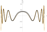
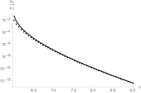
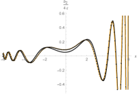
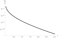
Figure 15: Plots of $b_{1}(x,6,4,0.03)/0.12$ (left, dots), $b_{2}(x,6,4,0.03)/0.12$ (right, dots), their analytic approximation from Theorem 7 (light), the imaginary part of the Feynman propagator $\mathrm{Im}\,G^{F}_{11}(x,6)$ (left, dark) and $\mathrm{Im}\,G^{F}_{12}(x,6)$ (right, dark) given by (34) for $m=4$ and $t=6$.

Definition 5.

(Cf. Proposition 12, see Figure 15.) Fix $m,\varepsilon>0$. For each $(x,t)\in\varepsilon\mathbb{Z}^{2}$ denote $\omega_{p}:=\frac{1}{\varepsilon}\arccos(\frac{\cos p\varepsilon}{\sqrt{1+m^{2}\varepsilon^{2}}})$ and

$$A_{1}(x,t,m,\varepsilon) :=\pm\frac{im\varepsilon^{2}}{2\pi}\int_{-\pi/\varepsilon}^{\pi/\varepsilon}\frac{e^{ipx-i\omega_{p}(t-\varepsilon)}\,dp}{\sqrt{m^{2}\varepsilon^{2}+\sin^{2}(p\varepsilon)}};$$ (32)

$$A_{2}(x,t,m,\varepsilon) :=\pm\frac{\varepsilon}{2\pi}\int_{-\pi/\varepsilon}^{\pi/\varepsilon}\left(1+\frac{\sin(p\varepsilon)}{\sqrt{m^{2}\varepsilon^{2}+\sin^{2}(p\varepsilon)}}\right)e^{ip(x-\varepsilon)-i\omega_{p}(t-\varepsilon)}\,dp,$$

where in both cases the overall minus sign is taken when $t\leq 0$ and $(x+t)/\varepsilon$ is even. For $m=0$ define $A_{2}(x,t,m,\varepsilon)$ by the same formula and set $A_{1}(x,t,0,\varepsilon):=0$. In particular, $A_{k}(x,t,m,\varepsilon)=a_{k}(x,t,m,\varepsilon)$ for $(x+t)/\varepsilon$ even, $t>0$, and $k=1,2$. Denote $A_{k}(x,t,m,\varepsilon)=:ib_{k}(x,t,m,\varepsilon)$ for $(x+t)/\varepsilon$ odd. Set $b_{k}(x,t,m,\varepsilon):=0$ for $(x+t)/\varepsilon$ even.

One can show that $A_{k}(x,t,m,\varepsilon)$ is purely imaginary for $(x+t)/\varepsilon$ odd. Thus the real and the imaginary parts ‘‘live’’ on the black and white squares respectively, analogously to how discrete analytic functions are defined (see [8]). The sign convention for $t\leq 0$ is dictated by the analogy to continuum theory (see (33) and (35)).

Example 6.

The value $b_{1}(0,1,1,1)=\Gamma(\tfrac{1}{4})^{2}/(2\pi)^{3/2}=\tfrac{2}{\pi}K(i)=:G\approx 0.83463$ is the Gauss constant and $-b_{2}(0,1,1,1)=2\sqrt{2\pi}/\Gamma(\tfrac{1}{4})^{2}=\tfrac{2}{\pi}(E(i)-K(i))=1/\pi G=:L^{\prime}\approx 0.38138$ is the inverse lemniscate constant, where $K(z)$ and $E(z)$ are the complete elliptic integrals of the 1st and 2nd kind respectively (cf. [13, §6.1]).

The other values are even more complicated irrationalities (see Table 6).

$b_{1}(x,t,1,1)$
$2$ $\frac{G-L^{\prime}}{\sqrt{2}}$ $\frac{G-L^{\prime}}{\sqrt{2}}$ $\frac{7G-15L^{\prime}}{3\sqrt{2}}$ $1$ $G$ $G-2L^{\prime}$ $0$ $\frac{G-L^{\prime}}{\sqrt{2}}$ $\frac{G-L^{\prime}}{\sqrt{2}}$ $\frac{7G-15L^{\prime}}{3\sqrt{2}}$ $-1$ $-L^{\prime}$ $\frac{2G-3L^{\prime}}{3}$ $-1$ $0$ $1$ $2$ $3$
$b_{2}(x,t,1,1)$
$2$ $\frac{G-3L^{\prime}}{3\sqrt{2}}$ $\frac{-G-L^{\prime}}{\sqrt{2}}$ $\frac{-G+3L^{\prime}}{\sqrt{2}}$ $1$ $-L^{\prime}$ $L^{\prime}$ $0$ $\frac{G-3L^{\prime}}{\sqrt{2}}$ $\frac{G+L^{\prime}}{\sqrt{2}}$ $\frac{-G+3L^{\prime}}{3\sqrt{2}}$ $-1$ $G$ $\frac{G}{3}$ $-1$ $0$ $1$ $2$ $3$

Table 6: The values $b_{1}(x,t,1,1)$ and $b_{2}(x,t,1,1)$ for small $x,t$ (see Definition 5 and Example 6)

We announce that the analogues of Propositions 5–8 and 10 remain true literally, if $a_{1}$ and $a_{2}$ are replaced by $b_{1}$ and $b_{2}$ respectively (the assumption $t>0$ can then be dropped). As a consequence, $2^{(t-1)/2}b_{1}(x,t,1,1)$ and $2^{(t-1)/2}b_{2}(x,t,1,1)$ for all $(x,t)\in\mathbb{Z}^{2}$ are rational linear combinations of the Gauss constant $G$ and the inverse lemniscate constant $L^{\prime}$. In general, we announce that $b_{1}$ and $b_{2}$ can be ‘‘explicitly’’ expressed through Gauss hypergeometric function: for $m,\varepsilon>0$, $(x,t)\in\varepsilon\mathbb{Z}^{2}$ with $(x+t)/\varepsilon$ odd we get

$$b_{1}(x,t,m,\varepsilon) =\left({1+m^{2}\varepsilon^{2}}\right)^{\frac{1}{2}-\frac{t}{2\varepsilon}}(-m^{2}\varepsilon^{2})^{\frac{t-|x|}{2\varepsilon}-\frac{1}{2}}\binom{\frac{t+|x|}{2\varepsilon}-1}{|x|/\varepsilon}$$

$$\cdot{}_{2}F_{1}\left(1+\frac{|x|-t}{2\varepsilon},1+\frac{|x|-t}{2\varepsilon};1+\frac{|x|}{\varepsilon};-\frac{1}{m^{2}\varepsilon^{2}}\right),$$

$$b_{2}(x+\varepsilon,t+\varepsilon,m,\varepsilon) =\left({1+m^{2}\varepsilon^{2}}\right)^{-\frac{t}{2\varepsilon}}(m\varepsilon)^{\frac{t-|x|}{\varepsilon}}(-1)^{\frac{t-|x|}{2\varepsilon}+\frac{1}{2}}\binom{\frac{t+|x|}{2\varepsilon}-1+\theta(x)}{|x|/\varepsilon}\,{}$$

$$\cdot{}_{2}F_{1}\left(\frac{|x|-t}{2\varepsilon},1+\frac{|x|-t}{2\varepsilon};1+\frac{|x|}{\varepsilon};-\frac{1}{m^{2}\varepsilon^{2}}\right),\qquad\text{where }\theta(x):=\begin{cases}1,&\mbox{if }x\geq 0,\\ 0,&\mbox{if }x<0;\end{cases}$$

and ${}_{2}F_{1}(p,q;r;z)$ is the principal branch of the hypergeometric function. The idea of the proof is induction on $t/\varepsilon\geq 1$: the base is given by [19, 9.112, 9.131.1, 9.134.3, 9.137.15] and the step is given by the analogue of (3)–(4) for $b_{1}$ and $b_{2}$ plus [19, 9.137.11,12,18].

Remark 7.

(Cf. Remark 3) These expressions can be rewritten as the Jacobi functions of the second kind of half-integer order (see the definition in [49, (4.61.1)]). For instance, for each $(x,t)\in\varepsilon\mathbb{Z}^{2}$ such that $|x|>t$ and $(x+t)/\varepsilon$ is odd we have

$$b_{1}(x,t,m,\varepsilon)=\frac{2m\varepsilon}{\pi}\left({1+m^{2}\varepsilon^{2}}\right)^{(t/\varepsilon-1)/2}Q_{(|x|-t)/2\varepsilon}^{(0,t/\varepsilon-1)}(1+2m^{2}\varepsilon^{2}).$$

Remark 8.

The number $b_{1}(x,\varepsilon,m,\varepsilon)$ equals $(1+\sqrt{1+m^{2}\varepsilon^{2}})/m\varepsilon$ times the probability that a planar simple random walk over white squares dies at $(x,\varepsilon)$, if it starts at $(0,\varepsilon)$ and dies with the probability $1-1/\sqrt{1+m^{2}\varepsilon^{2}}$ before each step. Nothing like that is known for $b_{1}(x,t,m,\varepsilon)$ and $b_{2}(x,t,m,\varepsilon)$ with $t\neq\varepsilon$.

The following two results are proved almost literally as Proposition 13 and Theorem 2. (The only difference is change of the sign of the summands involving $f_{-}(p)$ in (41), (46) (50), (52); the analogues of Lemmas 5 and 11 are then obtained by direct checking.)

Proposition 17 (Full space-time Fourier transform).

Denote $\delta_{x\varepsilon}:=1$, if $x=\varepsilon$, and $\delta_{x\varepsilon}:=0$, if $x\neq\varepsilon$. For each $m>0$ and $(x,t)\in\varepsilon\mathbb{Z}^{2}$ we get

$$A_{1}(x,t,m,\varepsilon) =\lim_{\delta\to+0}\frac{m\varepsilon^{3}}{4\pi^{2}}\int_{-\pi/\varepsilon}^{\pi/\varepsilon}\int_{-\pi/\varepsilon}^{\pi/\varepsilon}\frac{e^{ipx-i\omega(t-\varepsilon)}\,d\omega dp}{\sqrt{1+m^{2}\varepsilon^{2}}\cos(\omega\varepsilon)-\cos(p\varepsilon)-i\delta},$$ (33)

$$A_{2}(x,t,m,\varepsilon) =\lim_{\delta\to+0}\frac{-i\varepsilon^{2}}{4\pi^{2}}\int_{-\pi/\varepsilon}^{\pi/\varepsilon}\int_{-\pi/\varepsilon}^{\pi/\varepsilon}\frac{\sqrt{1+m^{2}\varepsilon^{2}}\sin(\omega\varepsilon)+\sin(p\varepsilon)}{\sqrt{1+m^{2}\varepsilon^{2}}\cos(\omega\varepsilon)-\cos(p\varepsilon)-i\delta}e^{ip(x-\varepsilon)-i\omega(t-\varepsilon)}\,d\omega dp+\delta_{x\varepsilon}\delta_{t\varepsilon}.$$

Theorem 7 (Large-time asymptotic formula between the peaks; see Figure 15).

For each $\delta>0$ there is $C_{\delta}>0$ such that for each $m,\varepsilon>0$ and each $(x,t)\in\varepsilon\mathbb{Z}^{2}$ satisfying (8) we have

$${b}_{1}\left(x,t+\varepsilon,m,\varepsilon\right) ={\varepsilon}\sqrt{\frac{2m}{\pi}}\left(t^{2}-(1+m^{2}\varepsilon^{2})x^{2}\right)^{-1/4}\cos\theta(x,t,m,\varepsilon)+O_{\delta}\left(\frac{\varepsilon}{m^{1/2}t^{3/2}}\right),$$

$${b}_{2}\left(x+\varepsilon,t+\varepsilon,m,\varepsilon\right) =-{\varepsilon}\sqrt{\frac{2m}{\pi}}\left(t^{2}-(1+m^{2}\varepsilon^{2})x^{2}\right)^{-1/4}\sqrt{\frac{t+x}{t-x}}\sin\theta(x,t,m,\varepsilon)+O_{\delta}\left(\frac{\varepsilon}{m^{1/2}t^{3/2}}\right),$$

for $(x+t)/\varepsilon$ even and odd respectively, where $\theta(x,t,m,\varepsilon)$ is given by (11).

9.2 Physical interpretation

One interprets $\frac{1}{2}|{A}_{1}\left(x,t,m,\varepsilon\right)|^{2}+\frac{1}{2}|{A}_{2}\left(x,t,m,\varepsilon\right)|^{2}$ as the expected charge in a square $(x,t)$ with $t>0$, in the units of electron charge. The numbers cannot be anymore interpreted as probabilities to find the electron in the square. The reason is that now the outcomes of the experiment are not mutually exclusive: one can detect an electron in two distinct squares simultaneously. There is nothing mysterious about that: Any measurement necessarily influences the electron. This influence might be enough to create an electron-positron pair from the vacuum. Thus one can detect a newborn electron in addition to the initial one; and there is no way to distinguish one from another. (A more formal explanation for specialists: two states in the Fock space representing the electron localized at distant regions are not mutually orthogonal; their scalar product is essentially provided by the Feynman propagator.)

We announce that the model reproduces the Feynman propagator rather than the retarded one in the continuum limit (see Figure 15). The spin-$1/2$ Feynman propagator equals

$$G^{F}(x,t)=\begin{cases}\dfrac{m}{4}\,\begin{pmatrix}J_{0}(ms)-iY_{0}(ms)&-{\frac{t+x}{s}}\left(J_{1}(ms)-iY_{1}(ms)\right)\\ {\frac{t-x}{s}}\left(J_{1}(ms)-iY_{1}(ms)\right)&J_{0}(ms)-iY_{0}(ms)\end{pmatrix},&\text{if }|x|<|t|;\\ \dfrac{im}{2\pi}\,\begin{pmatrix}K_{0}(ms)&{\frac{t+x}{s}}\,K_{1}(ms)\\ {\frac{x-t}{s}}\,K_{1}(ms)&K_{0}(ms)\end{pmatrix},&\text{if }|x|>|t|;\end{cases}$$ (34)

where $Y_{n}(z)$ and $K_{n}(z)$ are Bessel functions of the 2nd kind and modified Bessel functions of the 2nd kind, and $s:=\sqrt{\left|t^{2}-x^{2}\right|}$. In addition, there is a generalized function supported on the lines $t=\pm x$, which we do not specify. The Feynman propagator satisfies (25). We see that it has additional imaginary part (and an overall factor of $1/2$) compared to retarded one (26). In particular, it does not vanish for $|x|>|t|$: annihilation of electron at one point and creation at another one may result in apparent motion faster than light.

A more common expression is the Fourier transform (cf. (27) and [14, (6.51)])

$$G^{F}(x,t)=\frac{1}{4\pi^{2}}\int_{-\infty}^{+\infty}\int_{-\infty}^{+\infty}\lim_{\delta\to+0}\begin{pmatrix}m&-ip-i\omega\\ -ip+i\omega&m\end{pmatrix}\frac{e^{ipx-i\omega t}\,dpd\omega}{m^{2}+p^{2}-\omega^{2}-i\delta}.$$ (35)

Overall, a small correction introduced by the upgrade reflects some fundamental limitations on measurement rather than adds something meaningful to description of the motion. The upgrade should only be viewed as an ingredient for more realistic models with interaction.

9.3 Combinatorial definition

Informally, the combinatorial definition of Feynman anti-checkers (Definition 6) is obtained from the definition of Feynman checkers (Definition 2) by the following four-step modification:

Step 1:

the particle mass acquires small imaginary part which we eventually tend to zero;

Step 2:

just like the real mass is ‘‘responsible’’ for turns in the centers of the squares, the imaginary one allows turns at their vertices (see Figure 16 to the left);

Step 3:

the infinite lattice is replaced by a torus with the size eventually tending to infinity;

Step 4:

the sum over lattice paths is replaced by a ratio of sums over loop configurations.

Here Step 2 is completely new whereas the other ones are standard. It reflects a general principle that the real and the imaginary part of a quantity should be always put on dual lattices.

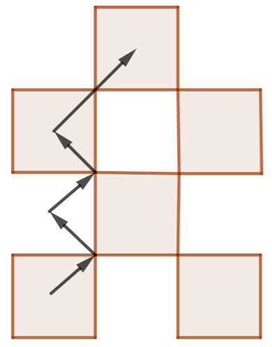
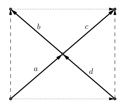
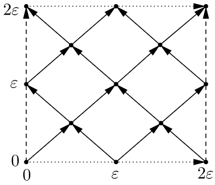
Figure 16: A generalized checker path (left) and lattices of sizes $1$ and $2$ (right); see Example 7.

Definition 6.

(see Figure 16) Fix $T\in\mathbb{Z}$ and $\varepsilon,m,\delta>0$ called lattice size, lattice step, particle mass, and small imaginary mass respectively. Assume $T>0$ and $\delta<1/2$. The lattice is the quotient set

$$\faktor{\{\,(x,t)\in[0,T\varepsilon]^{2}:2x/\varepsilon,2t/\varepsilon,(x+t)/\varepsilon\in\mathbb{Z}\,\}}{\forall x,t:(x,0)\sim(x,T\varepsilon)\,\&\,(0,t)\sim(T\varepsilon,t).}$$

(This is a finite subset of the torus obtained from the square $[0,T\varepsilon]^{2}$ by an identification of the opposite sides.) A lattice point $(x,t)$ is even (respectively, odd), if $2x/\varepsilon$ is even (respectively, odd). An edge is a vector starting from a lattice point $(x,t)$ and ending at the lattice point $(x+\varepsilon/2,t+\varepsilon/2)$ or $(x-\varepsilon/2,t+\varepsilon/2)$.

A generalized checker path is a finite sequence of distinct edges such that the endpoint of each edge is the starting point of the next one. A cycle is defined analogously, only the sequence has the unique repetition: the first and the last edges coincide, and there is at least one edge in between. (In particular, a generalized checker path such that the endpoint of the last edge is the starting point of the first one is not yet a cycle; coincidence of the first and the last edges is required. The first and the last edges of a generalized checker path coincide only if the path has a single edge. Thus in our setup, a path is never a cycle.) Changing the starting edge of a cycle means removal of the first edge from the sequence, then a cyclic permutation, and then adding the last edge of the resulting sequence at the beginning. A loop is a cycle up to changing of the starting edge.

A node of a path or loop $s$ is an ordered pair of consecutive edges in $s$ (the order of the edges in the pair is the same as in $s$). A turn is a node such that the two edges are orthogonal. A node or turn is even (respectively, odd), if the endpoint of the first edge in the pair is even (respectively, odd). Denote by $\mathrm{eventurns}(s)$, $\mathrm{oddturns}(s)$, $\mathrm{evennodes}(s)$, $\mathrm{oddnodes}(s)$ the number of even and odd turns and nodes in $s$. The arrow (or weight) of $s$ is

$${A}(s,m,\varepsilon,\delta):=\pm\frac{(-im\varepsilon)^{\mathrm{oddturns}(s)}(-\delta)^{\mathrm{eventurns}(s)}}{(1+m^{2}\varepsilon^{2})^{\mathrm{oddnodes}(s)/2}(1-\delta^{2})^{\mathrm{evennodes}(s)/2}},$$

where the overall minus sign is taken when $s$ is a loop.

A set of checker paths or loops is edge-disjoint, if no two of them have a common edge. An edge-disjoint set of loops is a loop configuration. A loop configuration with a source $a$ and a sink $f$ is an edge-disjoint set of any number of loops and exactly one generalized checker path starting with the edge $a$ and ending with the edge $f$. The arrow $A(S,m,\varepsilon,\delta)$ of a loop configuration $S$ (possibly with a source and a sink) is the product of arrows of all loops and paths in the configuration. An empty product is set to be $1$.

The arrow from an edge $a$ to an edge $f$ (or finite-lattice propagator) is

$${A}(a\to f,m,\varepsilon,\delta,T):=\frac{\sum\limits_{\begin{subarray}{c}\text{loop configurations $S$}\\ \text{with the source $a$ and the sink $f$}\end{subarray}}A(S,m,\varepsilon,\delta)}{\sum\limits_{\begin{subarray}{c}\text{loop configurations $S$}\end{subarray}}A(S,m,\varepsilon,\delta)}.$$

Now take a point $(x,t)\in(\varepsilon\mathbb{Z})^{2}$ and set $x^{\prime}:=x\mod T\varepsilon$, $t^{\prime}:=t\mod T\varepsilon$. Let $a_{0},f_{1},f_{2}$ be the edges starting at $(0,0)$, $(x^{\prime},t^{\prime})$, $(x^{\prime},t^{\prime})$ and ending at $(\varepsilon/2,\varepsilon/2)$, $(x^{\prime}-\varepsilon/2,t^{\prime}+\varepsilon/2)$, $(x^{\prime}+\varepsilon/2,t^{\prime}+\varepsilon/2)$ respectively. The arrow of the point $(x,t)$ (or infinite-lattice propagator) is the pair of complex numbers

$$\widetilde{A}_{k}(x,t,m,\varepsilon):=-2(-i)^{k}\,\lim_{\delta\searrow 0}\lim_{\begin{subarray}{c}T\to\infty\end{subarray}}{A}(a_{0}\to f_{k},m,\varepsilon,\delta,T)\qquad\text{for $k=1,2$.}$$

Example 7.

(See Figure 16 to the middle) The lattice of size $1$ lies on the square $[0,\varepsilon]^{2}$ with the opposite sides identified. The lattice has $2$ points: the midpoint and the identified vertices of the square. It has $4$ edges $a,b,c,d$. The generalized checker paths $abdc$, $acdb$, $bacd$ are distinct although they contain the same edges. Their arrows are $\tfrac{-m^{2}\varepsilon^{2}}{\sqrt{1-\delta^{2}}(1+m^{2}\varepsilon^{2})}$, $\tfrac{-\delta}{\sqrt{1-\delta^{2}}(1+m^{2}\varepsilon^{2})}$, $\tfrac{\delta^{2}}{(1-\delta^{2})\sqrt{1+m^{2}\varepsilon^{2}}}$ respectively. Those paths are distinct from the cycles $acdba$, $bacdb$. The two cycles determine the same loop with the arrow $\tfrac{-\delta^{2}}{(1-\delta^{2})(1+m^{2}\varepsilon^{2})}$. There are totally $9$ loop configurations: $\varnothing$, $\{aba\}$, $\{cdc\}$, $\{aca\}$, $\{bdb\}$, $\{abdca\}$, $\{acdba\}$, $\{aba,cdc\}$, $\{aca,bdb\}$. Their arrows are $1$, ${-im\varepsilon\delta}/n$, ${-im\varepsilon\delta}/n$, ${-1}/n$, ${-1}/n$, ${m^{2}\varepsilon^{2}}/n^{2}$, ${-\delta^{2}}/n^{2}$, ${-m^{2}\varepsilon^{2}\delta^{2}}/n^{2}$, ${1}/n^{2}$ respectively, where $n:={\sqrt{1-\delta^{2}}\sqrt{1+m^{2}\varepsilon^{2}}}$.

Informally, the loops form the Dirac sea of electrons filling the whole space, and the edges not in the loops form paths of holes in the sea, that is, antiparticles.

We announce that Definitions 5 and 6 are equivalent in the sense that $\widetilde{A}_{1}(x,t,m,\varepsilon)={A}_{1}(x,t+\varepsilon,m,\varepsilon)$ and $\widetilde{A}_{2}(x,t,m,\varepsilon)={A}_{2}(x+\varepsilon,t+\varepsilon,m,\varepsilon)$; cf. §6. The idea is that both definitions actually construct matrix elements of the ‘‘inverse’’ of the same lattice Dirac operator: the former via the Fourier transform, and the latter via the ratio of determinants.

10 Towards $(1+1)$-dimensional quantum electrodynamics

 Question: what is the probability to find electrons (or an electron and a positron) with momenta $q$ and $q^{\prime}$ in the far future, if they were emitted with momenta $p$ and $p^{\prime}$ in the far past?

Assumptions: interaction now switched on; all simplifying assumptions removed except the default ones:
no nuclear forces, no gravitation, electron moves along the $x$-axis only, and the $t$-axis is time.

Results: repulsion of like charges and attraction of opposite charges (qualitative explanation expected).  

Construction of the required model is a widely open problem because in particular it requires the missing mathematically rigorous construction of the Minkowskian lattice gauge theory.

11 Open problems

We start with problems relying on Definition 1. The plots suggest that for fixed $t$, the most probable position of the electron is near to $x=t/\sqrt{2}$ (see Figure 9 to the left, Theorems 1(B) and 2). Although this was noticed 20 years ago, the following question is still open.

Problem 1.

(A.Daniyarkhodzhaev–F.Kuyanov; see Figure 9 to the left) Denote by $x_{\max}(t)$ a point where $P(x,t)$ has a maximum for fixed $t$. Is $x_{\max}(t)-t/\sqrt{2}$ bounded as $t\to\infty$?

What makes the problem hard is that the behavior of $P(x,t)$ is only known near to $x=t/\sqrt{2}$ (Theorem 3) and far from $x=t/\sqrt{2}$ (Theorems 2 and 4) but not at intermediate distances.

Problem 2.

(Cf. [47]) Find a asymptotic formula for $P(x,t)$ as $t\to\infty$ uniform in $x\in[-t;t]$.

Problem 3.

(S. Nechaev; see Figure 9 to the left) Find the positions of ‘‘wide gaps’’ (intervals, where oscillations are smaller) in the plot of $P(x,t)$ for fixed large $t$. (Cf. formulae (9)–(10).)

The aim of the next two problems is to study the phase transition by means of various order parameters (see page 11). Specifically, we conjecture that the limiting ‘‘probability’’ of equal signs at the endpoints of the spin-chain, as well as the limiting ‘‘probability’’ of equal signs at the endpoints and the midpoint, are nonanalytic at $v=\pm 1/\sqrt{2}$.

Problem 4.

(See Figure 10) Prove that for each $0<v<1/\sqrt{2}$ we have

$$\lim_{t\to\infty}\sum\limits_{0\leq x\leq vt}\frac{2}{t}\left|\frac{a_{2}(x,t)}{a(x,t)}\right|^{2}=\frac{1}{2}\left(1+v-\sqrt{1-v^{2}}+\log\frac{1+\sqrt{1-v^{2}}}{2}\right).$$

Compute the same limit for $1/\sqrt{2}<v<1$. (Cf. the proof of Corollary 1 in §12.4.)

Problem 5.

(Cf. [23, p. 381].) Find the weak limit $\lim_{t\to\infty}\left|\sum_{x\in\mathbb{Z}}\dfrac{a_{2}(x,t)^{2}}{a_{2}(2\lceil vt\rceil-1,2t-1)}\right|^{2}$.

The next problem is on absorption probabilities; it relies on the definition before Example 1.

Problem 6.

(G. Minaev–I. Russkikh; cf. [1, §5], [10], [37, §4]) Find $\sum_{t=1}^{\infty}P(n,t\,\text{bypass}\,\{x\!\!=\!\!n\})$ for all $n\in\mathbb{Z}$. Find the weak limit and an asymptotic formula for $P(x,t\text{ bypass }\{x=0\})$ as $t\to\infty$. (Cf. Theorems 1–2.)

The following problem generalizes and specifies Problem 1 above; it relies on Definition 2.

Problem 7.

(A.Daniyarkhodzhaev–F.Kuyanov, cf. [1, §4], [47], [52]) Denote by $x_{\max}=x_{\max}(t,m,\varepsilon)$ the point where $P(x):=P(x,t,m,\varepsilon)$ has a maximum. Is $x_{\max}/\varepsilon-t/\varepsilon\sqrt{1+m^{2}\varepsilon^{2}}$ uniformly bounded? Does $P(x)$ decrease for $x>x_{\max}$? Find an asymptotic formula for $a(x,t,m,\varepsilon)$ as $t\to\infty$ valid for all $x\in[-t,t]$ and uniform in $x,m,\varepsilon$.

Problem 8.

(M. Blank–S. Shlosman) Is the number of times the function $a_{1}(x):=a_{1}(x,t,m,\varepsilon)$ changes the sign on $[-t,t]$ bounded as $\varepsilon\to 0$ for fixed $t,m$?

Corollary 6 gives uniform limit on compact subsets of the angle $|x|<t$, hence misses the main contribution to the probability. Now we ask for the weak limit detecting the peak.

Problem 9.

Find the weak limits $\lim\limits_{\varepsilon\to 0}\frac{1}{2\varepsilon}\,{a}\left(2\varepsilon\!\left\lceil\frac{x}{2\varepsilon}\right\rceil,2\varepsilon\!\left\lceil\frac{t}{2\varepsilon}\right\rceil,{m},{\varepsilon}\right)$ and $\lim\limits_{\varepsilon\to 0}\frac{1}{4\varepsilon^{2}}\,{P}\left(2\varepsilon\!\left\lceil\frac{x}{2\varepsilon}\right\rceil,2\varepsilon\!\left\lceil\frac{t}{2\varepsilon}\right\rceil,{m},{\varepsilon}\right)$ on the whole $\mathbb{R}^{2}$. Is the former limit equal to propagator (27) including the generalized function supported on the lines $t=\pm x$? What is the physical interpretation of the latter limit (providing a value to the ill-defined square of the propagator)?

The following problem is to construct a continuum analogue of Feynman checkers.

Problem 10.

(M. Lifshits) Consider $(-im\varepsilon)^{\mathrm{turns}(s)}$ as a charge on the set of all checker paths $s$ from $(0,0)$ to $(x,t)$ starting and ending with an upwards-right move. Does the charge converge (weakly or in another sense) to a charge on the space of all continuous functions $[0,t]\to\mathbb{R}$ with boundary values $0$ and $x$ respectively as $\varepsilon\to 0$?

The following problem relying on Definition 3 would demonstrate ‘‘spin precession’’.

Problem 11.

(See Figure 13 to the right; cf. [40]) Is $P(x)=\sum_{x\in\mathbb{Z}}a_{1}(x,t,u)^{2}$ a periodic function asymptotically as $t\to\infty$ for $u(x+\tfrac{1}{2},t+\tfrac{1}{2})=(-1)^{(x-1)(t-1)}$? Find the weak limit of $P(x,t,u)$ and asymptotic formulae for $a_{k}(x,t,u)$ as $t\to\infty$. (Cf. Theorems 1–2.)

Define ${a}(x,t,m,\varepsilon,u)$ analogously to ${a}(x,t,m,\varepsilon)$ and ${a}(x,t,u)$, unifying Definitions 2–3 and Remark 5. The next problem asks if this reproduces Dirac equation in electromagnetic field.

Problem 12.

(Cf. [16]) Fix $A_{0}(x,t),A_{1}(x,t)\in C^{2}(\mathbb{R}^{2})$. For each auxiliary edge $s_{1}s_{2}$ set

$$u(s_{1}s_{2}):=\exp\left(-i\int_{s_{1}}^{s_{2}}\left(A_{0}(x,t)\,dt+A_{1}(x,t)\,dx\right)\right).$$

Denote $\psi_{k}(x,t):=\lim_{\varepsilon\to 0}\frac{1}{2\varepsilon}\,{a}_{k}\left(2\varepsilon\!\left\lceil\frac{x}{2\varepsilon}\right\rceil,2\varepsilon\!\left\lceil\frac{t}{2\varepsilon}\right\rceil,{m},{\varepsilon},u\right)$ for $k=1,2$. Does the limit satisfy

$$\begin{pmatrix}m&\partial/\partial x-\partial/\partial t+iA_{0}(x,t)-iA_{1}(x,t)\\ \partial/\partial x+\partial/\partial t-iA_{0}(x,t)-iA_{1}(x,t)&m\end{pmatrix}\begin{pmatrix}\psi_{2}(x,t)\\ \psi_{1}(x,t)\end{pmatrix}=0\quad\text{for }t>0?$$

The next two problems rely on Definition 5.

Problem 13.

(Cf. Corollary 1) Prove that $\lim\limits_{\begin{subarray}{c}t\to\infty\\ t\in\varepsilon\mathbb{Z}\end{subarray}}\sum\limits_{\begin{subarray}{c}x\leq vt\\ x\in\varepsilon\mathbb{Z}\end{subarray}}\dfrac{\left|A_{1}(x,t,{m},{\varepsilon})\right|^{2}+\left|A_{2}(x,t,{m},{\varepsilon})\right|^{2}}{2}=F(v,m,\varepsilon)$.

Problem 14.

(Cf. Theorems 4 and 7) Find an asymptotic formula for $A_{k}(x,t,{m},{\varepsilon})$ for $|x|>|t|$ as $t\to\infty$.

The last problem is informal; it stands for half a century.

Problem 15.

(R. Feynman; cf. [15]) Generalize the model to $4$ dimensions so that

$$\lim_{\varepsilon\to 0}\frac{1}{2\varepsilon}\,{a}\left(2\varepsilon\!\left\lceil\frac{x}{2\varepsilon}\right\rceil,2\varepsilon\!\left\lceil\frac{y}{2\varepsilon}\right\rceil,2\varepsilon\!\left\lceil\frac{z}{2\varepsilon}\right\rceil,2\varepsilon\!\left\lceil\frac{t}{2\varepsilon}\right\rceil,{m},{\varepsilon}\right)$$

coincides with the spin-$1/2$ retarded propagator, now in $3$ space- and $1$ time-dimension.

12 Proofs

Let us present a chart showing the dependence of the above results and further subsections:

Particular proposition numbers are shown above the arrows. Propositions 7, 10, and 13 are not used in the main results.

In the process of the proofs, we give a zero-knowledge introduction to the used methods. Some proofs are simpler than the original ones.

12.1 Identities: elementary combinatorics (Propositions 1–13)

Let us prove the identities from §3; the ones from §2 are the particular case $m=\varepsilon=1$.

Proof of Propositions 1 and 5.

Let us derive a recurrence for $a_{2}(x,t,m,\varepsilon)$. Take a path $s$ on $\varepsilon\mathbb{Z}^{2}$ from $(0,0)$ to $(x,t)$ with the first step to $(\varepsilon,\varepsilon)$. Set $a(s,m\varepsilon):=i(-im\varepsilon)^{\mathrm{turns}(s)}(1+m^{2}\varepsilon^{2})^{(1-t/\varepsilon)/2}$.

The last move in the path $s$ is made either from $(x-\varepsilon,t-\varepsilon)$ or from $(x+\varepsilon,t-\varepsilon)$. If it is from $(x+\varepsilon,t-\varepsilon)$, then $\mathrm{turns}(s)$ must be odd, hence $s$ does not contribute to $a_{2}(x,t,m,\varepsilon)$. Assume further that the last move in $s$ is made from $(x-\varepsilon,t-\varepsilon)$. Denote by $s^{\prime}$ the path $s$ without the last move. If the directions of the last moves in $s$ and $s^{\prime}$ coincide, then $a(s,m\varepsilon)=\frac{1}{\sqrt{1+m^{2}\varepsilon^{2}}}a(s^{\prime},m\varepsilon)$, otherwise $a(s,m\varepsilon)=\frac{-im\varepsilon}{\sqrt{1+m^{2}\varepsilon^{2}}}a(s^{\prime},m\varepsilon)=\frac{m\varepsilon}{\sqrt{1+m^{2}\varepsilon^{2}}}(\mathrm{Im}\,a(s^{\prime},m\varepsilon)-i\mathrm{Re}\,a(s^{\prime},m\varepsilon))$.

Summation over all paths $s^{\prime}$ gives the required equation

$$a_{2}(x,t,m,\varepsilon)=\mathrm{Im}\sum_{s\ni(x-\varepsilon,t-\varepsilon)}a(s,m\varepsilon)=\sum_{s^{\prime}\ni(x-2\varepsilon,t-2\varepsilon)}\frac{\mathrm{Im}\,a(s^{\prime},m\varepsilon)}{\sqrt{1+m^{2}\varepsilon^{2}}}-\sum_{s^{\prime}\ni(x,t-2\varepsilon)}\frac{m\varepsilon\,\mathrm{Re}\,a(s^{\prime},m\varepsilon)}{\sqrt{1+m^{2}\varepsilon^{2}}}\\ =\frac{1}{\sqrt{1+m^{2}\varepsilon^{2}}}\left(a_{2}(x-\varepsilon,t-\varepsilon,m,\varepsilon)-m\varepsilon\,a_{1}(x-\varepsilon,t-\varepsilon,m,\varepsilon)\right).$$

The recurrence for $a_{1}(x,t+\varepsilon,m,\varepsilon)$ is proved analogously. ∎

Proof of Propositions 2 and 6.

The proof is by induction on $t/\varepsilon$. The base $t/\varepsilon=1$ is obvious. The step of induction follows immediately from the following computation using Proposition 5:

$$\sum\limits_{x\varepsilon\in\mathbb{Z}}P(x,t+\varepsilon,m,\varepsilon)=\sum\limits_{x\in\varepsilon\mathbb{Z}}\left[a_{1}(x,t+\varepsilon,m,\varepsilon)^{2}+a_{2}(x,t+\varepsilon,m,\varepsilon)^{2}\right]\\ =\tfrac{1}{1+m^{2}\varepsilon^{2}}\left(\sum\limits_{x\in\varepsilon\mathbb{Z}}[a_{1}(x+\varepsilon,t,m,\varepsilon)+m\varepsilon\,a_{2}(x+\varepsilon,t,m,\varepsilon)]^{2}+\sum\limits_{x\in\varepsilon\mathbb{Z}}[a_{2}(x-\varepsilon,t,m,\varepsilon)-m\varepsilon\,a_{1}(x-\varepsilon,t,m,\varepsilon)]^{2}\right)\\ =\tfrac{1}{1+m^{2}\varepsilon^{2}}\left(\sum\limits_{x\in\varepsilon\mathbb{Z}}[a_{1}(x,t,m,\varepsilon)+m\varepsilon\,a_{2}(x,t,m,\varepsilon)]^{2}+\sum\limits_{x\in\varepsilon\mathbb{Z}}[a_{2}(x,t,m,\varepsilon)-m\varepsilon\,a_{1}(x,t,m,\varepsilon)]^{2}\right)\\ =\sum\limits_{x\in\varepsilon\mathbb{Z}}\left[a_{1}(x,t,m,\varepsilon)^{2}+a_{2}(x,t,m,\varepsilon)^{2}\right]=\sum\limits_{x\in\varepsilon\mathbb{Z}}P(x,t,m,\varepsilon).\\[-42.67912pt]$$

∎

Lemma 1 (Adjoint Dirac equation).

For each $(x,t)\in\varepsilon\mathbb{Z}^{2}$, where $t>\varepsilon$, we have

$$a_{1}(x,t-\varepsilon,m,\varepsilon) =\frac{1}{\sqrt{1+m^{2}\varepsilon^{2}}}(a_{1}(x-\varepsilon,t,m,\varepsilon)-m\varepsilon\,a_{2}(x+\varepsilon,t,m,\varepsilon));$$

$$a_{2}(x,t-\varepsilon,m,\varepsilon) =\frac{1}{\sqrt{1+m^{2}\varepsilon^{2}}}(m\varepsilon\,a_{1}(x-\varepsilon,t,m,\varepsilon)+a_{2}(x+\varepsilon,t,m,\varepsilon)).$$

Proof of Lemma 1.

The second equation is obtained from Proposition 5 by substituting $(x,t)$ by $(x-\varepsilon,t-\varepsilon)$ and $(x+\varepsilon,t-\varepsilon)$ in (3) and (4) respectively and adding them with the coefficients $m\varepsilon/\sqrt{1+m^{2}\varepsilon^{2}}$ and $1/\sqrt{1+m^{2}\varepsilon^{2}}$. The first equation is obtained analogously. ∎

Proof of Proposition 7.

The real part of the desired equation is the sum of the first equations of Lemma 1 and Proposition 5. The imaginary part is the sum of the second ones. ∎

Proof of Proposition 8.

Let us prove the first identity. For a path $s$ denote by $s^{\prime}$ the reflection of $s$ with respect to the $t$ axis, and by $s^{\prime\prime}$ the path consisting of the same moves as $s^{\prime}$, but in the opposite order.

Take a path $s$ from $(0,0)$ to $(x,t)$ with the first move upwards-right such that $\mathrm{turns}(s)$ is odd (the ones with $\mathrm{turns}(s)$ even do not contribute to $a_{1}(x,t,m,\varepsilon)$). Then the last move in $s$ is upwards-left. Therefore, the last move in $s^{\prime}$ is upwards-right, hence the first move in $s^{\prime\prime}$ is upwards-right. The endpoint of both $s^{\prime}$ and $s^{\prime\prime}$ is $(-x,t)$, because reordering of moves does not affect the endpoint. Thus $s\mapsto s^{\prime\prime}$ is a bijection between the paths to $(x,t)$ and to $(-x,t)$ with $\mathrm{turns}(s)$ odd. Thus $a_{1}(x,t,m,\varepsilon)=a_{1}(-x,t,m,\varepsilon)$.

We prove the second identity by induction on $t/\varepsilon$ (this proof was found and written by E. Kolpakov). The base of induction ($t/\varepsilon=1$ and $t/\varepsilon=2$) is obvious.

Step of induction: take $t\geq 3\varepsilon$. Applying the inductive hypothesis for the three points $(x-\varepsilon,t-\varepsilon),(x+\varepsilon,t-\varepsilon),(x,t-2\varepsilon)$ and the identity just proved, we get

$$(t-x)a_{2}(x-\varepsilon,t-\varepsilon,m,\varepsilon) =(x+t-4\varepsilon)a_{2}(3\varepsilon-x,t-\varepsilon,m,\varepsilon),$$

$$(t-x-2\varepsilon)a_{2}(x+\varepsilon,t-\varepsilon,m,\varepsilon) =(x+t-2\varepsilon)a_{2}(\varepsilon-x,t-\varepsilon,m,\varepsilon),$$

$$(t-x-2\varepsilon)a_{2}(x,t-2\varepsilon,m,\varepsilon) =(x+t-4\varepsilon)a_{2}(2\varepsilon-x,t-2\varepsilon,m,\varepsilon),$$

$$a_{1}(x-\varepsilon,t-\varepsilon,m,\varepsilon) =a_{1}(\varepsilon-x,t-\varepsilon,m,\varepsilon).$$

Summing up the $4$ equations with the coefficients $1,1,-\sqrt{1+m^{2}\varepsilon^{2}},-2m\varepsilon^{2}$ respectively, we get

$$(t-x)\left(a_{2}(x-\varepsilon,t-\varepsilon,m,\varepsilon)+a_{2}(x+\varepsilon,t-\varepsilon,m,\varepsilon)-\sqrt{1+m^{2}\varepsilon^{2}}\,a_{2}(x,t-2\varepsilon,m,\varepsilon)\right)\\ -2m\varepsilon^{2}\,a_{1}(x-\varepsilon,t-\varepsilon,m,\varepsilon)-2\varepsilon\,a_{2}(x+\varepsilon,t-\varepsilon,m,\varepsilon)+2\varepsilon\sqrt{1+m^{2}\varepsilon^{2}}\,a_{2}(x,t-2\varepsilon,m,\varepsilon)=\\ =-2m\varepsilon^{2}\,a_{1}(\varepsilon-x,t-\varepsilon,m,\varepsilon)-2\varepsilon\,a_{2}(3\varepsilon-x,t-\varepsilon,m,\varepsilon)+2\varepsilon\sqrt{1+m^{2}\varepsilon^{2}}\,a_{2}(2\varepsilon-x,t-2\varepsilon,m,\varepsilon)\\ +(t+x-2\varepsilon)\left(a_{2}(3\varepsilon-x,t-\varepsilon,m,\varepsilon)+a_{2}(\varepsilon-x,t-\varepsilon,m,\varepsilon)-\sqrt{1+m^{2}\varepsilon^{2}}\,a_{2}(2\varepsilon-x,t-2\varepsilon,m,\varepsilon)\right).$$

Here the 3 terms in the 2nd line, as well as the 3 terms in the 3rd line, cancel each other by Lemma 1. Applying the Klein–Gordon equation (Proposition 7) to the expressions in the 1st and 4th line and cancelling the common factor $\sqrt{1+m^{2}\varepsilon^{2}}$, we get the desired identity

$$(t-x)a_{2}(x,t,m,\varepsilon)=(t+x-2\varepsilon)a_{2}(2\varepsilon-x,t,m,\varepsilon).$$

The third identity follows from the first one and Proposition 5:

$$a_{1}(x,t,m,\varepsilon)+m\varepsilon\,a_{2}(x,t,m,\varepsilon)=\sqrt{1+m^{2}\varepsilon^{2}}\,a_{1}(x-\varepsilon,t+\varepsilon,m,\varepsilon)=\\ =\sqrt{1+m^{2}\varepsilon^{2}}\,a_{1}(\varepsilon-x,t+\varepsilon,m,\varepsilon)=a_{1}(2\varepsilon-x,t,m,\varepsilon)+m\varepsilon\,a_{2}(2\varepsilon-x,t,m,\varepsilon).\\[-42.67912pt]$$

∎

The 1st and the 3rd identities can also be proved simultaneously by induction on $t/\varepsilon$ using Proposition 5.

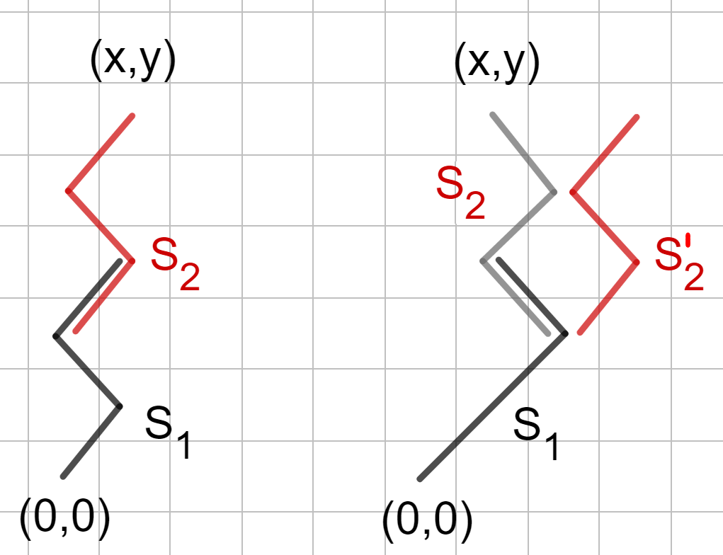
Figure 17: The path cut into two parts (see the proof of Proposition 9).

Proof of Proposition 9.

Take a checker path $s$ from $(0,0)$ to $(x,t)$. Denote by $(x^{\prime},t^{\prime})$ the point where $s$ intersects the line $t=t^{\prime}$. Denote by $s_{1}$ the part of $s$ that joins $(0,0)$ with $(x^{\prime},t^{\prime})$. Denote by $s_{2}$ the part starting at the intersection point of $s$ with the line $t=t^{\prime}-\varepsilon$ and ending at $(x,t)$ (see Figure 17). Translate the path $s_{2}$ so that it starts at $(0,0)$. Set $a(s,m\varepsilon):=i(-im\varepsilon)^{\mathrm{turns}(s)}(1+m^{2}\varepsilon^{2})^{(1-t/\varepsilon)/2}$. Since $\mathrm{turns}(s)=\mathrm{turns}(s_{1})+\mathrm{turns}(s_{2})$, it follows that

$$\mathrm{Re}\,a(s,m\varepsilon)=\begin{cases}\mathrm{Re}\,a(s_{1},m\varepsilon)\mathrm{Im}\,a(s_{2},m\varepsilon),&\text{if the move to $(x^{\prime},t^{\prime})$ is upwards-left},\\ \mathrm{Im}\,a(s_{1},m\varepsilon)\mathrm{Re}\,a(s_{2},m\varepsilon),&\text{if the move to $(x^{\prime},t^{\prime})$ is upwards-right}.\end{cases}$$

In the former case replace the path $s_{2}$ by the path $s_{2}^{\prime}$ obtained by the reflection with respect to the line $x=0$ (and starting at the origin). We have $\mathrm{Im}\,a(s_{2}^{\prime},m\varepsilon)=\mathrm{Im}\,a(s_{2},m\varepsilon)$. Therefore,

$$a_{1}(x,t,m,\varepsilon)=\sum\limits_{s}\mathrm{Re}\,a(s,m\varepsilon)=\sum\limits_{x^{\prime}}\sum\limits_{s\ni(x^{\prime},t^{\prime})}\mathrm{Re}\,a(s,m\varepsilon)\\ =\sum\limits_{x^{\prime}}\left(\sum\limits_{s\ni(x^{\prime},t^{\prime}),(x^{\prime}-\varepsilon,t^{\prime}-\varepsilon)}\mathrm{Im}\,a(s_{1},m\varepsilon)\mathrm{Re}\,a(s_{2},m\varepsilon)+\sum\limits_{s\ni(x^{\prime},t^{\prime}),(x^{\prime}+\varepsilon,t^{\prime}-\varepsilon)}\mathrm{Re}\,a(s_{1},m\varepsilon)\mathrm{Im}\,a(s_{2}^{\prime},m\varepsilon)\right)\\ =\sum\limits_{x^{\prime}}\left[a_{2}(x^{\prime},t^{\prime},m,\varepsilon)a_{1}(x-x^{\prime}+\varepsilon,t-t^{\prime}+\varepsilon,m,\varepsilon)+a_{1}(x^{\prime},t^{\prime},m,\varepsilon)a_{2}(x^{\prime}-x+\varepsilon,t-t^{\prime}+\varepsilon,m,\varepsilon)\right].$$

The formula for $a_{2}(x,t,m,\varepsilon)$ is proven analogously. ∎

Proof of Proposition 10.

Denote by $f(x,t)$ the difference between the left- and the right-hand side of (5). Introduce the operator

$$[\square_{m}f](x,t):=\sqrt{1+m^{2}\varepsilon^{2}}\,f(x,t+\varepsilon)+\sqrt{1+m^{2}\varepsilon^{2}}\,f(x,t-\varepsilon)-f(x+\varepsilon,t)-f(x-\varepsilon,t).$$

It suffices to prove that

$$[\square_{m}^{4}f](x,t)=0\qquad\text{for }t\geq 5\varepsilon.$$ (36)

Then (5) will follow by induction on $t/\varepsilon$: (36) expresses $f(x,t+4\varepsilon)$ as a linear combination of $f(x^{\prime},t^{\prime})$ with smaller $t^{\prime}$; it remains to check $f(x,t)=0$ for $t\leq 8\varepsilon$, which is done in [44, §11].

To prove (36), write

$$f(x,t)=:p_{1}(x,t)a(x-2\varepsilon,t,m,\varepsilon)+p_{2}(x,t)a(x+2\varepsilon,t,m,\varepsilon)+p_{3}(x,t)a(x,t,m,\varepsilon)$$

for certain cubic polynomials $p_{k}(x,t)$ (see (5)), and observe the Leibnitz rule

$$\square_{m}(fg)=f\cdot\square_{m}g+\sqrt{1+m^{2}\varepsilon^{2}}(\nabla_{t+}f\cdot T_{t+}g-\nabla_{t-}f\cdot T_{t-}g)-\nabla_{x+}f\cdot T_{x+}g+\nabla_{x-}f\cdot T_{x-}g,$$

where $[\nabla_{t\pm}f](x,t):=\pm(f(x,t\pm\varepsilon)-f(x,t))$ and $[\nabla_{x\pm}f](x,t):=\pm(f(x\pm\varepsilon,t)-f(x,t))$ are the finite difference operators, $[T_{t\pm}g](x,t):=g(x,t\pm\varepsilon)$ and $[T_{x\pm}g](x,t):=g(x\pm\varepsilon,t)$ are the shift operators. Since $\square_{m}\,a(x,t,m,\varepsilon)=0$ by Proposition 7, each operator $\nabla_{t\pm},\nabla_{x\pm}$ decreases $\deg p_{k}(x,t)$, and all the above operators commute, by the Leibnitz rule we get (36). This proves the first identity in the proposition; the second one is proved analogously (the induction base is checked in [44, §11]). ∎

Alternatively, Proposition 10 can be derived by applying the Gauss contiguous relations to the hypergeometric expression from Remark 3 seven times.

Proof of Propositions 3 and 11.

Let us find $a_{1}(x,t,m,\varepsilon)$. Consider a path with an odd number of turns; the other ones do not contribute to $a_{1}(x,t,m,\varepsilon)$. Denote by $2r+1$ the number of turns in the path. Denote by $R$ and $L$ the number of upwards-right and upwards-left moves respectively. Let $x_{1},x_{2},\dots,x_{r+1}$ be the number of upwards-right moves before the first, the third, …, the last turn respectively. Let $y_{1},y_{2},\dots,y_{r+1}$ be the number of upwards-left moves after the first, the third, …, the last turn respectively. Then $x_{k},y_{k}\geq 1$ for $1\leq k\leq r+1$ and

$$R =x_{1}+\dots+x_{r+1};$$

$$L =y_{1}+\dots+y_{r+1}.$$

The problem now reduces to a combinatorial one: the number of paths with $2r+1$ turns equals the number of positive integer solutions of the resulting equations. For the first equation, this number is the number of ways to put $r$ sticks between $R$ coins in a row, that is, $\binom{R-1}{r}$. Thus

$$a_{1}(x,t,m,\varepsilon)=(1+m^{2}\varepsilon^{2})^{(1-t/\varepsilon)/2}\sum_{r=0}^{\min\{R,L\}}(-1)^{r}\binom{R-1}{r}\binom{L-1}{r}(m\varepsilon)^{2r+1}.$$

Thus (6) follows from $L+R=t/\varepsilon$ and $R-L=x/\varepsilon$. Formula (7) is derived analogously. ∎

Proof of Proposition 12.

The proof is by induction on $t/\varepsilon$.

The base $t/\varepsilon=1$ is obtained by the change of variable $p\mapsto p+\pi/\varepsilon$ so that the integrals over $[0;\pi/\varepsilon]$ and $[-\pi/\varepsilon;0]$ cancel for $x/\varepsilon$ odd and there remains $(\varepsilon/2\pi)\int_{-\pi/\varepsilon}^{\pi/\varepsilon}e^{ip(x-\varepsilon)}=\delta_{x\varepsilon}$.

The inductive step is the following computation and an analogous one for $a_{2}(x,t+\varepsilon,m,\varepsilon)$:

$$a_{1}(x,t+\varepsilon,m,\varepsilon)=\frac{1}{\sqrt{1+m^{2}\varepsilon^{2}}}\left(a_{1}(x+\varepsilon,t,m,\varepsilon)+m\varepsilon\,a_{2}(x+\varepsilon,t,m,\varepsilon)\right)\\ =\frac{m\varepsilon^{2}}{2\pi\sqrt{1+m^{2}\varepsilon^{2}}}\int_{-\pi/\varepsilon}^{\pi/\varepsilon}\left(\frac{ie^{ip\varepsilon}}{\sqrt{m^{2}\varepsilon^{2}+\sin^{2}(p\varepsilon)}}+1+\frac{\sin(p\varepsilon)}{\sqrt{m^{2}\varepsilon^{2}+\sin^{2}(p\varepsilon)}}\right)e^{ipx-i\omega_{p}(t-\varepsilon)}\,dp\\ =\frac{m\varepsilon^{2}}{2\pi}\int_{-\pi/\varepsilon}^{\pi/\varepsilon}\frac{\left(i\cos(\omega_{p}\varepsilon)+\sin(\omega_{p}\varepsilon)\right)e^{ipx-i\omega_{p}(t-\varepsilon)}\,dp}{\sqrt{m^{2}\varepsilon^{2}+\sin^{2}(p\varepsilon)}}=\frac{im\varepsilon^{2}}{2\pi}\int_{-\pi/\varepsilon}^{\pi/\varepsilon}\frac{e^{ipx-i\omega_{p}t}\,dp}{\sqrt{m^{2}\varepsilon^{2}+\sin^{2}(p\varepsilon)}}.$$

Here the 1st equality is Proposition 5. The 2nd one is the inductive hypothesis. The 3rd one follows from $\cos\omega_{p}\varepsilon=\frac{\cos p\varepsilon}{\sqrt{1+m^{2}\varepsilon^{2}}}$ and $\sin\omega_{p}\varepsilon=\sqrt{1-\frac{\cos^{2}p\varepsilon}{1+m^{2}\varepsilon^{2}}}=\sqrt{\frac{m^{2}\varepsilon^{2}+\sin^{2}p\varepsilon}{1+m^{2}\varepsilon^{2}}}$. ∎

Alternatively, Proposition 12 can be derived by integration of (30)–(31) over $p=2\pi/\lambda$ for $\tilde{a}_{1}(0,0)=0$, $\tilde{a}_{2}(0,0)=1$.

Proof of Proposition 13.

To prove the formula for $a_{1}(x,t,m,\varepsilon)$, we do the $\omega$-integral:

$$\frac{\varepsilon}{2\pi}\int\limits_{-\pi/\varepsilon}^{\pi/\varepsilon}\frac{e^{-i\omega(t-\varepsilon)}\,d\omega}{\sqrt{1+m^{2}\varepsilon^{2}}\cos(\omega\varepsilon)-\cos(p\varepsilon)-i\delta}\overset{(*)}{=}\frac{1}{2\pi i}\oint\limits_{|z|=1}\frac{2\,z^{t/\varepsilon-1}\,dz}{\sqrt{1+m^{2}\varepsilon^{2}}z^{2}-2(\cos(p\varepsilon)+i\delta)z+\sqrt{1+m^{2}\varepsilon^{2}}}\\ \overset{(**)}{=}\frac{\left(\left(\cos p\varepsilon+i\delta-i\sqrt{m^{2}\varepsilon^{2}+\sin^{2}p\varepsilon+\delta^{2}-2i\delta\cos p\varepsilon}\right)/\sqrt{1+m^{2}\varepsilon^{2}}\right)^{t/\varepsilon-1}}{-i\sqrt{m^{2}\varepsilon^{2}+\sin^{2}p\varepsilon+\delta^{2}-2i\delta\cos p\varepsilon}}\overset{(***)}{\rightrightarrows}\frac{i\,e^{-i\omega_{p}(t-\varepsilon)}}{\sqrt{m^{2}\varepsilon^{2}+\sin^{2}p\varepsilon}}$$

as $\delta\to 0$ uniformly in $p$. Here we assume that $m,t,\delta>0$ and $\delta$ is sufficiently small. Equality $(*)$ is obtained by the change of variables $z=e^{-i\omega\varepsilon}$ and then the change of the contour direction to the counterclockwise one. To prove $(**)$, we find the roots of the denominator

$$z_{\pm}=\frac{\cos p\varepsilon+i\delta\pm i\sqrt{m^{2}\varepsilon^{2}+\sin^{2}p\varepsilon+\delta^{2}-2i\delta\cos p\varepsilon}}{\sqrt{1+m^{2}\varepsilon^{2}}},$$

where $\sqrt{z}$ denotes the value of the square root with positive real part. Then $(**)$ follows from the residue formula: the expansion

$$z_{\pm}=\frac{\cos p\varepsilon\pm i\sqrt{m^{2}\varepsilon^{2}+\sin^{2}p\varepsilon}}{\sqrt{1+m^{2}\varepsilon^{2}}}\left(1\pm\frac{\delta}{\sqrt{m^{2}\varepsilon^{2}+\sin^{2}p\varepsilon}}+{O}_{m,\varepsilon}\left(\delta^{2}\right)\right)$$

shows that $z_{-}$ is inside the unit circle, whereas $z_{+}$ is outside, for $\delta>0$ sufficiently small in terms of $m$ and $\varepsilon$. In $(***)$ we denote $\omega_{p}:=\frac{1}{\varepsilon}\arccos(\frac{\cos p\varepsilon}{\sqrt{1+m^{2}\varepsilon^{2}}})$ so that $\sin\omega_{p}\varepsilon=\sqrt{\frac{m^{2}\varepsilon^{2}+\sin^{2}p\varepsilon}{1+m^{2}\varepsilon^{2}}}$ and pass to the limit $\delta\to 0$ which is uniform in $p$ by the assumption $m>0$.

The resulting uniform convergence allows to interchange the limit and the $p$-integral, and we arrive at Fourier integral for $a_{1}(x,t,m,\varepsilon)$ in Proposition 12. The formula for $a_{2}(x,t,m,\varepsilon)$ is proved analogously, with the case $t=\varepsilon$ considered separately. ∎

12.2 Phase transition: the method of moments (Theorem 1)

In this subsection we give a simple exposition of the proof of Theorem 1 from [20] using the method of moments. The theorem also follows from Corollary 1 obtained by another method in §12.4. We rely on the following well-known result.

Lemma 2.

(See [5, Theorems 30.1–30.2]) Let $f_{t}\colon\mathbb{R}\to[0,+\infty)$, where $t=0,1,2,\dots$, be piecewise continuous functions such that $\alpha_{r,t}:=\int_{-\infty}^{+\infty}v^{r}f_{t}(v)\,dv$ is finite and $\alpha_{0,t}=1$ for each $r,t=0,1,2,\dots$. If the series $\sum_{r=0}^{\infty}\alpha_{r,0}z^{r}/r!$ has positive radius of convergence and $\lim_{t\to\infty}\alpha_{r,t}=\alpha_{r,0}$ for each $r=0,1,2,\dots$, then $f_{t}$ converges to $f_{0}$ in distribution.

Proof of Theorem 1.

Let us prove (C); then (A) and (B) will follow from Lemma 2 for $f_{0}(v):=F^{\prime}(v)$ and $f_{t}(v):=tP(\lceil vt\rceil,t)$ because $F^{\prime}(v)=0$ for $|v|>1$, hence $\alpha_{r,0}\leq\int_{-1}^{+1}|F^{\prime}(v)|\,dv=1$.

Rewrite Proposition 12 in a form, valid for each $x,t\in\mathbb{Z}$ independently on the parity:

$$\begin{pmatrix}a_{1}(x,t)\\ a_{2}(x,t)\end{pmatrix}=\int_{-\pi}^{\pi}\begin{pmatrix}\hat{a}_{1}(p,t)\\ \hat{a}_{2}(p,t)\end{pmatrix}e^{ip(x-1)}\,\frac{dp}{2\pi}:=\int_{-\pi}^{\pi}\begin{pmatrix}\hat{a}_{1+}(p,t)+\hat{a}_{1-}(p,t)\\ \hat{a}_{2+}(p,t)+\hat{a}_{2-}(p,t)\end{pmatrix}e^{ip(x-1)}\,\frac{dp}{2\pi},$$ (37)

where

$$\hat{a}_{1\pm}(p,t) =\mp\frac{ie^{ip}}{2\sqrt{1+\sin^{2}p}}e^{\pm i\omega_{p}(t-1)};$$ (38)

$$\hat{a}_{2\pm}(p,t) =\frac{1}{2}\left(1\mp\frac{\sin p}{\sqrt{1+\sin^{2}p}}\right)e^{\pm i\omega_{p}(t-1)};$$

and $\omega_{p}:=\arccos\frac{\cos p}{\sqrt{2}}$. Now (37) holds for each $x,t\in\mathbb{Z}$: Indeed, the identity

$$\exp\left({-i\omega_{p+\pi}(t-1)+i(p+\pi)(x-1)}\right)=\exp\left({-i(\pi-\omega_{p})(t-1)+ip(x-1)+i\pi(x-1)}\right)=\\ =(-1)^{(x+t)}\exp\left({i\omega_{p}(t-1)+ip(x-1)}\right)$$

shows that the contributions of the two summands $\hat{a}_{k\pm}(p,t)$ to integral (37) are equal for $t+x$ even and cancel for $t+x$ odd. The summand $\hat{a}_{k-}(p,t)$ contributes $a_{k}(x,t)/2$ by Proposition 12.

By the derivative property of Fourier series and the Parseval theorem, we have

$$\sum_{x\in\mathbb{Z}}\frac{x^{r}}{t^{r}}P(x,t)=\sum_{x\in\mathbb{Z}}\begin{pmatrix}a_{1}(x,t)\\ a_{2}(x,t)\end{pmatrix}^{*}\frac{x^{r}}{t^{r}}\begin{pmatrix}a_{1}(x,t)\\ a_{2}(x,t)\end{pmatrix}=\int\limits_{-\pi}^{\pi}\begin{pmatrix}\hat{a}_{1}(p,t)\\ \hat{a}_{2}(p,t)\end{pmatrix}^{*}\frac{i^{r}}{t^{r}}\frac{\partial^{r}}{\partial p^{r}}\begin{pmatrix}\hat{a}_{1}(p,t)\\ \hat{a}_{2}(p,t)\end{pmatrix}\,\frac{dp}{2\pi}.$$ (39)

The derivative is estimated as follows:

$$\frac{\partial^{r}}{\partial p^{r}}\hat{a}_{k\pm}(p,t)=\left(\pm i(t-1)\frac{\partial\omega_{p}}{\partial p}\right)^{r}\hat{a}_{k\pm}(p,t)+O_{r}(t^{r-1})=\left(\pm\frac{i(t-1)\sin p}{\sqrt{1+\sin^{2}p}}\right)^{r}\hat{a}_{k\pm}(p,t)+O_{r}(t^{r-1}).$$ (40)

Indeed, differentiate (38) $r$ times using the Leibnitz rule. If we differentiate the exponential factor $e^{\pm i\omega_{p}(t-1)}$ each time, then we get the main term. If we differentiate a factor rather than the exponential $e^{\pm i\omega_{p}(t-1)}$ at least once, then we get less than $r$ factors of $(t-1)$, hence the resulting term is $O_{r}(t^{r-1})$ by compactness because it is continuous and $2\pi$-periodic in $p$.

Substituting (40) into (39) we arrive at

$$\sum_{x\in\mathbb{Z}}\frac{x^{r}}{t^{r}}P(x,t)=\int_{-\pi}^{\pi}\begin{pmatrix}\hat{a}_{1}(p,t)\\ \hat{a}_{2}(p,t)\end{pmatrix}^{*}\left(\frac{\sin p}{\sqrt{1+\sin^{2}p}}\right)^{r}\begin{pmatrix}(-1)^{r}\hat{a}_{1+}(p,t)+\hat{a}_{1-}(p,t)\\ (-1)^{r}\hat{a}_{2+}(p,t)+\hat{a}_{2-}(p,t)\end{pmatrix}\,\frac{dp}{2\pi}+O_{r}\left(\frac{1}{t}\right)\\ =\int_{-\pi}^{\pi}\left(\frac{\sin p}{\sqrt{1+\sin^{2}p}}\right)^{r}\frac{1}{2}\left((-1)^{r}\left(1-\frac{\sin p}{\sqrt{1+\sin^{2}p}}\right)+1+\frac{\sin p}{\sqrt{1+\sin^{2}p}}\right)\,\frac{dp}{2\pi}+O_{r}\left(\frac{1}{t}\right)\\ =\int_{-\pi/2}^{\pi/2}\left(\frac{\sin p}{\sqrt{1+\sin^{2}p}}\right)^{r}\left(1+\frac{\sin p}{\sqrt{1+\sin^{2}p}}\right)\,\frac{dp}{\pi}+O_{r}\left(\frac{1}{t}\right)=\int_{-1/\sqrt{2}}^{1/\sqrt{2}}\frac{v^{r}\,dv}{\pi(1-v)\sqrt{1-2v^{2}}}+O_{r}\left(\frac{1}{t}\right).$$

Here the 2nd equality follows from $\hat{a}_{1\pm}(p,t)^{*}\hat{a}_{1\pm}(p,t)+\hat{a}_{2\pm}(p,t)^{*}\hat{a}_{2\pm}(p,t)=\frac{1}{2}\left(1\mp\frac{\sin p}{\sqrt{1+\sin^{2}p}}\right)$ and $\hat{a}_{1\pm}(p,t)^{*}\hat{a}_{1\mp}(p,t)+\hat{a}_{2\pm}(p,t)^{*}\hat{a}_{2\mp}(p,t)=0$. The 3rd one is obtained by the changes of variables $p\mapsto-p$ and $p\mapsto\pi-p$ applied to the integral over $[-\pi/2,\pi/2]$. The 4th one is obtained by the change of variables $v=\sin p/\sqrt{1+\sin^{2}p}$ so that $dp=d\arcsin\frac{v}{\sqrt{1-v^{2}}}=dv/(1-v^{2})\sqrt{1-2v^{2}}$. ∎

12.3 The main result: the stationary phase method (Theorem 2)

In this subsection we prove Theorem 2. First we outline the plan of the argument, then prove the theorem modulo some technical lemmas, and finally the lemmas themselves.

The plan is to apply the Fourier transform and the stationary phase method to the resulting oscillatory integral. The proof has $4$ steps, with the first two known before ([1, §4], [47, §2]):

Step 1:

computing the main term in the asymptotic formula;

Step 2:

estimating approximation error arising from neighborhoods of stationary points;

Step 3:

estimating approximation error arising from a neighborhood of the origin;

Step 4:

estimating error arising from the complements to those neighborhoods.

Proof of Theorem 2 modulo some lemmas.

Derive the asymptotic formula for $a_{1}\left(x,t+\varepsilon,{m},{\varepsilon}\right)$; the derivation for $a_{2}\left(x+\varepsilon,t+\varepsilon,{m},{\varepsilon}\right)$ is analogous and is discussed at the end of the proof. By Proposition 12 and the identity $e^{i\omega_{p+\pi/\varepsilon}t-i(p+\pi/\varepsilon)x}=e^{i(\pi/\varepsilon-\omega_{p})t-ipx-i\pi x/\varepsilon}=-e^{-i\omega_{p}t-ipx}$ for $(t+x)/\varepsilon$ odd, we get

$$a_{1}(x,t+\varepsilon,m,\varepsilon)=\frac{m\varepsilon^{2}}{2\pi i}\int_{-\pi/\varepsilon}^{\pi/\varepsilon}\frac{e^{i\omega_{p}t-ipx}}{\sqrt{m^{2}\varepsilon^{2}+\sin^{2}(p\varepsilon)}}\,dp=\int_{-\pi/2\varepsilon}^{\pi/2\varepsilon}g(p)(e(f_{+}(p))-e(f_{-}(p)))\,dp,$$ (41)

where $e(z):=e^{2\pi iz}$ and

$$f_{\pm}(p) =\frac{1}{2\pi}\left(-px\pm\frac{t}{\varepsilon}\arccos\frac{\cos(p\varepsilon)}{\sqrt{1+m^{2}\varepsilon^{2}}}\right),$$ (42)

$$g(p) =\frac{m\varepsilon^{2}}{2\pi i\sqrt{m^{2}\varepsilon^{2}+\sin^{2}(p\varepsilon)}}.$$ (43)

Step 1. We estimate oscillatory integral (41) using the following known technical result.

Lemma 3 (Weighted stationary phase integral).

[21, Lemma 5.5.6] Let $f(p)$ be a real function, four times continuously differentiable for $\alpha\leq p\leq\beta$, and let $g(p)$ be a real function, three times continuously differentiable for $\alpha\leq p\leq\beta$. Suppose that there are positive parameters $M,N,T,U$, with

$$M\geq\beta-\alpha,\qquad N\geq M/\sqrt{T},$$

and positive constants $C_{r}$ such that, for $\alpha\leq p\leq\beta$,

$$\left|f^{(r)}(p)\right|\leq C_{r}T/M^{r},\qquad\left|g^{(s)}(p)\right|\leq C_{s}U/N^{s},$$

for $r=2,3,4$ and $s=0,1,2,3$, and

$$f^{\prime\prime}(p)\geq T/C_{2}M^{2}.$$

Suppose also that $f^{\prime}(p)$ changes sign from negative to positive at a point $p=\gamma$ with $\alpha<\gamma<\beta$. If $T$ is sufficiently large in terms of the constants $C_{r}$, then we have

$$\int_{\alpha}^{\beta}g(p)e(f(p))\,dp=\frac{g(\gamma)e(f(\gamma)+1/8)}{\sqrt{f^{\prime\prime}(\gamma)}}+\frac{g(\beta)e(f(\beta))}{2\pi if^{\prime}(\beta)}-\frac{g(\alpha)e(f(\alpha))}{2\pi if^{\prime}(\alpha)}\\ +{O}_{C_{0},\dots,C_{4}}\left(\frac{M^{4}U}{T^{2}}\left(1+\frac{M}{N}\right)^{2}\left(\frac{1}{(\gamma-\alpha)^{3}}+\frac{1}{(\beta-\gamma)^{3}}+\frac{\sqrt{T}}{M^{3}}\right)\right).$$ (44)

Here the first term involving the values at the stationary point $\gamma$ is the main term, and the boundary terms involving the values at the endpoints $\alpha$ and $\beta$ are going to cancel out in Step 3.

Lemma 4.

(Cf. [23, (25)], [1, §4]) Assume (8); then on $[-\frac{\pi}{2\varepsilon},\frac{\pi}{2\varepsilon}]$, the function $f_{\pm}(p)$ given by (42) has a unique critical point

$$\gamma_{\pm}=\pm\frac{1}{\varepsilon}\arcsin\frac{m\varepsilon x}{\sqrt{t^{2}-x^{2}}}.$$ (45)

To estimate integral (41), we are going to apply Lemma 3 twice, for the functions $f(p)=\pm f_{\pm}(p)$ in appropriate neighborhoods of their critical points $\gamma_{\pm}$. In the case of $f(p)=-f_{-}(p)$, we perform complex conjugation of both sides of (44). Then the total contribution of the two resulting main terms is

$$\mathrm{MainTerm}:=\frac{g(\gamma_{+})e(f_{+}(\gamma_{+})+1/8)}{\sqrt{f_{+}^{\prime\prime}(\gamma_{+})}}-\frac{g(\gamma_{-})e(f_{-}(\gamma_{-})-1/8)}{\sqrt{-f_{-}^{\prime\prime}(\gamma_{-})}}.$$ (46)

A direct but long computation (see [44, §2]) then gives the desired main term in the theorem:

Lemma 5.

(See [44, §2]) Assume (8), (11), (42)–(43), (45); then expression (46) equals

$$\mathrm{MainTerm}=\varepsilon\sqrt{\frac{2m}{\pi}}\left(t^{2}-(1+m^{2}\varepsilon^{2})x^{2}\right)^{-1/4}\sin\theta(x,t,m,\varepsilon).$$

Step 2. To estimate the approximation error, we need to specify the particular values of parameters which Lemma 3 is applied for:

$$M =N=m, T =mt, U =\varepsilon.$$ (47)

Lemma 6.

If $\varepsilon\leq 1/m$ then functions (42)–(43) and parameters (47) satisfy the inequalities

$$\left|f_{\pm}^{(r)}(p)\right|\leq 3T/M^{r},\qquad\left|g^{(s)}(p)\right|\leq 3U/N^{s}\qquad\text{for $p\in\mathbb{R}$, \ $r=2,3,4$, \ $s=0,1,2,3$.}$$

We also need to specify the interval

$$[\alpha_{\pm},\beta_{\pm}]:=[\gamma_{\pm}-m\delta/2,\gamma_{\pm}+m\delta/2].$$ (48)

To estimate the derivative $|f_{\pm}^{\prime\prime}(p)|$ from below, we make sure that we are apart its roots $\pm\pi/2\varepsilon$.

Lemma 7.

Assume (8), (45); then interval (48) is contained in $[-\pi/2\varepsilon+m\delta/2,\pi/2\varepsilon-m\delta/2]$.

The wise choice of the interval provides the following more technical estimate.

Lemma 8.

Assume (8), (42), (45), and (48). Then for each $p\in[\alpha_{\pm},\beta_{\pm}]$ we have

$$|f_{\pm}^{\prime\prime}(p)|\geq\frac{t\delta^{3/2}}{24\pi m}.$$

This gives $|f_{\pm}^{\prime\prime}(p)|\geq T/C_{2}M^{2}$ for $C_{2}:=24\pi\delta^{-3/2}$ under notation (47). Now all the assumptions of Lemma 3 have been verified ($M\geq\beta_{\pm}-\alpha_{\pm}$ and $N\geq M/\sqrt{T}$ are automatic because $\delta\leq 1$ and $t>C_{\delta}/m$ by (8)). Apply the lemma to $g(p)$ and $\pm f_{\pm}(p)$ on $[\alpha_{\pm},\beta_{\pm}]$ (the minus sign before $f_{-}(p)$ guarantees the inequality $f^{\prime\prime}(p)>0$ and the factor of $i$ inside $g(p)$ is irrelevant for application of the lemma). We arrive at the following estimate for the approximation error on those intervals.

Lemma 9.

(See [44, §4]) Parameters (45) and (47)–(48) satisfy

$$\frac{M^{4}U}{T^{2}}\left(1+\frac{M}{N}\right)^{2}\left(\frac{1}{(\gamma_{\pm}-\alpha_{\pm})^{3}}+\frac{1}{(\beta_{\pm}-\gamma_{\pm})^{3}}+\frac{\sqrt{T}}{M^{3}}\right)={O}_{\delta}\left(\frac{\varepsilon}{m^{1/2}t^{3/2}}\right).$$

Although that is only a part of the error, it is already of the same order as in the theorem.

Step 3. To estimate the approximation error outside $[\alpha_{\pm},\beta_{\pm}]$, we use another known technical result.

Lemma 10 (Weighted first derivative test).

[21, Lemma 5.5.5] Let $f(p)$ be a real function, three times continuously differentiable for $\alpha\leq p\leq\beta$, and let $g(p)$ be a real function, twice continuously differentiable for $\alpha\leq p\leq\beta$. Suppose that there are positive parameters $M,N,T,U$, with $M\geq\beta-\alpha,$ and positive constants $C_{r}$ such that, for $\alpha\leq p\leq\beta$,

$$\left|f^{(r)}(p)\right|\leq C_{r}T/M^{r},\qquad\left|g^{(s)}(p)\right|\leq C_{s}U/N^{s},$$

for $r=2,3$ and $s=0,1,2$. If $f^{\prime}(p)$ and $f^{\prime\prime}(p)$ do not change sign on the interval $[\alpha,\beta]$, then

$$\int_{\alpha}^{\beta}g(p)e(f(p))\,dp=\frac{g(\beta)e(f(\beta))}{2\pi if^{\prime}(\beta)}-\frac{g(\alpha)e(f(\alpha))}{2\pi if^{\prime}(\alpha)}\\ +{O}_{C_{0},\dots,C_{3}}\left(\frac{TU}{M^{2}}\left(1+\frac{M}{N}+\frac{M^{3}\min|f^{\prime}(p)|}{N^{2}T}\right)\frac{1}{\min|f^{\prime}(p)|^{3}}\right).$$

This lemma in particular requires the interval to be sufficiently small. By this reason we decompose the initial interval $[-\pi/2\varepsilon,\pi/2\varepsilon]$ into a large number of intervals by the points

$$-\frac{\pi}{2\varepsilon}=\alpha_{-K}<\beta_{-K}=\alpha_{-K+1}<\beta_{-K+1}=\alpha_{-K+2}<\dots=\alpha_{i}<\hat{\beta}_{i}=\alpha_{\pm}<\beta_{\pm}=\hat{\alpha}_{j}<\beta_{j}=\dots<\beta_{K-1}=\frac{\pi}{2\varepsilon}.$$

Here $\alpha_{\pm}$ and $\beta_{\pm}$ are given by (48) above. The other points are given by

$$\alpha_{k}=\frac{k\pi}{2\varepsilon K},\quad\beta_{k}=\frac{(k+1)\pi}{2\varepsilon K},\quad\text{where}\quad K=2\left\lceil\frac{\pi}{m\varepsilon}\right\rceil\quad\text{and}\quad k=-K,\dots,i,j+1,\dots,K-1.$$ (49)

The indices $i$ and $j$ are the minimal ones such that $\frac{(i+1)\pi}{2\varepsilon K}>\alpha_{\pm}$ and $\frac{(j+1)\pi}{2\varepsilon K}>\beta_{\pm}$. Thus all the resulting intervals except $[\alpha_{\pm},\beta_{\pm}]$ and its neighbors have the same length $\frac{\pi}{2\varepsilon K}$. (Although it is more conceptual to decompose using a geometric sequence rather than arithmetic one, this does not affect the final estimate here.)

We have already applied Lemma 3 to $[\alpha_{\pm},\beta_{\pm}]$ and we are going to apply Lemma 10 to each of the remaining intervals in the decomposition for $f(p)=f_{\pm}(p)$ (this time it is not necessary to change the sign of $f_{-}(p)$). After summation of the resulting estimates, all the terms involving the values $f_{\pm}(\alpha_{k})$ and $f_{\pm}(\beta_{k})$ at the endpoints, except the leftmost and the rightmost ones, are going to cancel out. The remaining boundary terms give

$$\mathrm{BoundaryTerm}:=\frac{g(\frac{\pi}{2\varepsilon})e(f_{+}(\frac{\pi}{2\varepsilon}))}{2\pi if^{\prime}_{+}(\frac{\pi}{2\varepsilon})}-\frac{g(-\frac{\pi}{2\varepsilon})e(f_{+}(-\frac{\pi}{2\varepsilon}))}{2\pi if^{\prime}_{+}(-\frac{\pi}{2\varepsilon})}-\frac{g(\frac{\pi}{2\varepsilon})e(f_{-}(\frac{\pi}{2\varepsilon}))}{2\pi if^{\prime}_{-}(\frac{\pi}{2\varepsilon})}+\frac{g(-\frac{\pi}{2\varepsilon})e(f_{-}(-\frac{\pi}{2\varepsilon}))}{2\pi if^{\prime}_{-}(-\frac{\pi}{2\varepsilon})}.$$ (50)

Lemma 11.

(See [44, §5]) For $(x,t)\in\varepsilon\mathbb{Z}^{2}$ such that $(x+t)/\varepsilon$ is odd, expression (50) vanishes.

It remains to estimate the error terms. We start estimates with the central intervals $[\alpha_{0},\beta_{0}]$ and $[\alpha_{-1},\beta_{-1}]$ (possibly without parts cut out by $[\alpha_{\pm},\beta_{\pm}]$); they require a special treatment. Apply Lemma 10 to the intervals for the same functions (42)–(43) and the same values (47) of the parameters $M,N,T,U$ as in Step 2. All the assumptions of the lemma have been already verified in Lemma 6; we have $\beta_{0}-\alpha_{0}\leq{\pi}/{2\varepsilon K}={\pi}/4\varepsilon\lceil\frac{\pi}{m\varepsilon}\rceil<m=M$ and $f^{\prime\prime}_{\pm}(p)\neq 0$ as well. We are thus left to estimate $|f_{\pm}^{\prime}(p)|$ from below.

Lemma 12.

Assume (8), (42), (45), (48); then for each $p\in[-\pi/2\varepsilon,\pi/2\varepsilon]\setminus[\alpha_{\pm},\beta_{\pm}]$ we get

$$|f_{\pm}^{\prime}(p)|\geq t\delta^{5/2}/48\pi.$$

Then the approximation error on the central intervals is estimated as follows.

Lemma 13.

(See [44, §6]) Assume (8), (45), and (48). Then parameters (47) and functions (42) satisfy

$$\frac{TU}{M^{2}}\left(1+\frac{M}{N}+\frac{M^{3}\min_{p\in[\alpha_{\pm},\beta_{\pm}]}|f_{\pm}^{\prime}(p)|}{N^{2}T}\right)\frac{1}{\min_{p\in[\alpha_{\pm},\beta_{\pm}]}|f_{\pm}^{\prime}(p)|^{3}}={O}\left(\frac{\varepsilon}{mt^{2}\delta^{15/2}}\right).$$

This value is ${O}_{\delta}\left({\varepsilon}/{m^{1/2}t^{3/2}}\right)$ because $t>C_{\delta}/m$ by (8). Hence the approximation error on the central intervals is within the remainder of the theorem.

Step 4. To estimate the approximation error on the other intervals $[\alpha_{k},\beta_{k}]$, where we assume that $k>0$ without loss of generality, we apply Lemma 10 with slightly different parameters:

$$T =mt/k, M =mk, U =\varepsilon/k, N =mk.$$ (51)

Lemma 14.

For $0<k<K$ and $\varepsilon\leq 1/m$, parameters (51) and (49), functions (42)–(43) on $[\alpha_{k},\beta_{k}]$ satisfy all the assumptions of Lemma 10 possibly except the one on the sign of $f^{\prime}(p)$.

Since the neighborhood $[\alpha_{\pm},\beta_{\pm}]$ of the root of $f^{\prime}(p)$ is cut out, it follows that $f^{\prime}(p)$ has constant sign on the remaining intervals, and by Lemma 10 their contribution to the error is estimated as follows.

Lemma 15.

(See [44, §7]) Assume (8), (45), (48), $0<k<K$. Then functions (42) and parameters (51) satisfy

$$\frac{TU}{M^{2}}\left(1+\frac{M}{N}+\frac{M^{3}\min_{p\not\in[\alpha_{\pm},\beta_{\pm}]}|f_{\pm}^{\prime}(p)|}{N^{2}T}\right)\frac{1}{\min_{p\not\in[\alpha_{\pm},\beta_{\pm}]}|f_{\pm}^{\prime}(p)|^{3}}={O}\left(\frac{\varepsilon}{k^{2}mt^{2}\delta^{15/2}}\right).$$

Summation over all $k$ gives the approximation error

$$\sum_{k=1}^{K}{O}\left(\frac{\varepsilon}{k^{2}mt^{2}\delta^{15/2}}\right)={O}\left(\frac{\varepsilon}{mt^{2}\delta^{15/2}}\sum_{k=1}^{\infty}\frac{1}{k^{2}}\right)={O}_{\delta}\left(\frac{\varepsilon}{m^{1/2}t^{3/2}}\right).$$

because the series inside big-O converges and $t>C_{\delta}/m$. Thus the total approximation error on all the intervals is within the error term in the theorem, which completes the proof of (9).

The derivation of the asymptotic formula for $a_{2}\left(x+\varepsilon,t+\varepsilon,{m},{\varepsilon}\right)$ is analogous. By Proposition 12 for $(x+t)/\varepsilon$ even we get

$$a_{2}\left(x+\varepsilon,t+\varepsilon,{m},{\varepsilon}\right)=\frac{\varepsilon}{2\pi}\int_{-\pi/\varepsilon}^{\pi/\varepsilon}\left(1+\frac{\sin(p\varepsilon)}{\sqrt{m^{2}\varepsilon^{2}+\sin^{2}(p\varepsilon)}}\right)e^{i\omega_{p}t-ipx}\,dp\\ =\int_{-\pi/2\varepsilon}^{\pi/2\varepsilon}\left[g_{+}(p)e(f_{+}(p))+g_{-}(p)e(f_{-}(p))\right]dp,$$ (52)

where $f_{\pm}(p)$ are the same as above (see (42)) and

$$g_{\pm}(p) =\frac{\varepsilon}{2\pi}\left(1\pm\frac{\sin(p\varepsilon)}{\sqrt{m^{2}\varepsilon^{2}+\sin^{2}(p\varepsilon)}}\right).$$ (53)

One repeats the argument of Steps 1–4 with $g(p)$ replaced by $g_{\pm}(p)$. The particular form of $g(p)$ was only used in Lemmas 5, 6, 11, 14. The analogues of Lemmas 5 and 11 for $g_{\pm}(p)$ are obtained by direct checking [44, §13]. Lemma 6 holds for $g_{\pm}(p)$: one needs not to repeat the proof because $g_{\pm}(p)=(\varepsilon/t)(f_{\pm}^{\prime}(p)+(x+t)/2\pi)$ [44, §1]. But parameters (51) and Lemma 14 should be replaced by the following ones (then the analogue of Lemma 15 holds):

$$T =mt/k, M =mk, U =\varepsilon, N =mk^{3/2}.$$ (54)

Lemma 16.

For $0<k<K$ and $\varepsilon\leq 1/m$, parameters (54) and (49), functions (42) and (53) on $[\alpha_{k},\beta_{k}]$ satisfy all the assumptions of Lemma 10 possibly except the one on the sign of $f^{\prime}(p)$.

Again, one needs not to repeat the proof: Lemma 16 follows from Lemma 14 and the expression of $g_{\pm}$ through $f_{\pm}^{\prime}$.

This concludes the proof of Theorem 2 modulo the lemmas. ∎

Now we prove the lemmas. Lemmas 5, 9, 11, 13, 15 are proved by direct checking [44]. The following expressions [44, §1,3] are used frequently in the proofs of the other lemmas:

$$f_{\pm}^{\prime}(p) =\frac{1}{2\pi}\left(-x\pm\frac{t\sin p\varepsilon}{\sqrt{m^{2}\varepsilon^{2}+\sin^{2}p\varepsilon}}\right);$$ (55)

$$f_{\pm}^{\prime\prime}(p) =\pm\frac{m^{2}\varepsilon^{3}t\cos(p\varepsilon)}{2\pi\left(m^{2}\varepsilon^{2}+\sin^{2}(p\varepsilon)\right)^{3/2}}$$ (56)

Proof of Lemma 4.

Using (55) and solving the quadratic equation $f_{\pm}^{\prime}(p)=0$ in $\sin p\varepsilon$, we get (45). The assumption $|x|/t<1/\sqrt{1+m^{2}\varepsilon^{2}}$ from (8) guarantees that the arcsine exists. ∎

Proof of Lemma 6.

By the computation of the derivatives in [44, §3] and the assumption $m\varepsilon\leq 1$ we get

$$|g(p)| =\frac{m\varepsilon^{2}}{2\pi\sqrt{m^{2}\varepsilon^{2}+\sin^{2}(p\varepsilon)}}\leq\frac{m\varepsilon^{2}}{2\pi\sqrt{m^{2}\varepsilon^{2}+0}}\leq\varepsilon=U,$$

$$|g^{(1)}(p)| =\frac{m\varepsilon^{3}|\sin(p\varepsilon)\cos(p\varepsilon)|}{2\pi\left(m^{2}\varepsilon^{2}+\sin^{2}(p\varepsilon)\right)^{3/2}}\leq\frac{m\varepsilon^{3}|\sin(p\varepsilon)\cos(p\varepsilon)|}{2\pi\left(m^{2}\varepsilon^{2}+0\right)\left(0+\sin^{2}(p\varepsilon)\right)^{1/2}}\leq\frac{\varepsilon}{m}=\frac{U}{N},$$

$$|g^{(2)}(p)| =\frac{m\varepsilon^{4}\left|m^{2}\varepsilon^{2}+\sin^{4}(p\varepsilon)-2(1+m^{2}\varepsilon^{2})\sin^{2}(p\varepsilon)\right|}{2\pi\left(m^{2}\varepsilon^{2}+\sin^{2}(p\varepsilon)\right)^{5/2}}\leq\frac{m\varepsilon^{4}\left(3m^{2}\varepsilon^{2}+3\sin^{2}(p\varepsilon)\right)}{2\pi\left(m^{2}\varepsilon^{2}+\sin^{2}(p\varepsilon)\right)^{5/2}}\leq\frac{\varepsilon}{m^{2}}=\frac{U}{N^{2}},$$

$$|g^{(3)}(p)| =\frac{m\varepsilon^{5}|\sin(p\varepsilon)\cos(p\varepsilon)|\cdot\left|4m^{4}\varepsilon^{4}+9m^{2}\varepsilon^{2}+\sin^{4}(p\varepsilon)-(6+10m^{2}\varepsilon^{2})\sin^{2}(p\varepsilon)\right|}{2\pi\left(m^{2}\varepsilon^{2}+\sin^{2}(p\varepsilon)\right)^{7/2}}\leq\frac{3\varepsilon}{m^{3}}=\frac{3U}{N^{3}},$$

$$|f^{(2)}_{\pm}(p)| =\frac{m^{2}\varepsilon^{3}t\cos(p\varepsilon)}{2\pi\left(m^{2}\varepsilon^{2}+\sin^{2}(p\varepsilon)\right)^{3/2}}\leq\frac{t}{m}=\frac{T}{M^{2}},$$

$$|f^{(3)}_{\pm}(p)| =\frac{m^{2}\varepsilon^{4}t|\sin(p\varepsilon)|\left(m^{2}\varepsilon^{2}+\cos(2p\varepsilon)+2\right)}{2\pi\left(m^{2}\varepsilon^{2}+\sin^{2}(p\varepsilon)\right)^{5/2}}\leq\frac{4m^{2}\varepsilon^{4}t|\sin(p\varepsilon)|}{2\pi\left(m^{2}\varepsilon^{2}+\sin^{2}(p\varepsilon)\right)^{5/2}}\leq\frac{t}{m^{2}}=\frac{T}{M^{3}},$$

$$|f^{(4)}_{\pm}(p)| =\frac{m^{2}\varepsilon^{5}t\cos(p\varepsilon)\left|m^{4}\varepsilon^{4}+3m^{2}\varepsilon^{2}+4\sin^{4}(p\varepsilon)-2(6+5m^{2}\varepsilon^{2})\sin^{2}(p\varepsilon)\right|}{2\pi\left(m^{2}\varepsilon^{2}+\sin^{2}(p\varepsilon)\right)^{7/2}}\leq\frac{3t}{m^{3}}=\frac{3T}{M^{4}}.$$

∎

Proof of Lemma 7.

The lemma follows from the sequence of estimates

$$\frac{\pi}{2\varepsilon}-|\gamma_{\pm}|=\frac{\sin(\pi/2)-\sin|\gamma_{\pm}\varepsilon|}{\varepsilon\cos(\theta\varepsilon)}\geq\frac{\sin(\pi/2)-\sin|\gamma_{\pm}\varepsilon|}{\varepsilon\cos(\gamma_{\pm}\varepsilon)}=\frac{1-m\varepsilon|x|/\sqrt{t^{2}-x^{2}}}{\varepsilon\sqrt{1-m^{2}\varepsilon^{2}x^{2}/(t^{2}-x^{2})}}\\ =\frac{\sqrt{1-x^{2}/t^{2}}-m\varepsilon|x|/t}{\varepsilon\sqrt{1-(1+m^{2}\varepsilon^{2})x^{2}/t^{2}}}\geq\frac{1}{\varepsilon}\left(\sqrt{1-\frac{x^{2}}{t^{2}}}-\frac{m\varepsilon|x|}{t}\right)\\ \geq\frac{1}{\varepsilon}\left(\sqrt{1-\frac{1}{1+m^{2}\varepsilon^{2}}}-\frac{m\varepsilon|x|}{t}\right)=m\left(\frac{1}{\sqrt{1+m^{2}\varepsilon^{2}}}-\frac{|x|}{t}\right)\geq{m\delta}.$$

Here the first equality holds for some $\theta\in[|\gamma_{\pm}|,\pi/2\varepsilon]$ by the Lagrange theorem. The next inequality holds because the cosine is decreasing on the interval. The next one is obtained by substituting (45). The rest is straightforward because $|x|/t<1/\sqrt{1+m^{2}\varepsilon^{2}}-\delta$ by (8). ∎

Proof of Lemma 8.

Let us prove the lemma for $f_{+}(p)$ and $\gamma_{+}\geq 0$; the other signs are considered analogously. Omit the index $+$ in the notation of $f_{+},\alpha_{+},\beta_{+},\gamma_{+}$. The lemma follows from

$$|f^{(2)}(p)| \overset{(*)}{\geq}|f^{(2)}(\beta)|=\frac{m^{2}\varepsilon^{3}t\cos(\beta\varepsilon)}{2\pi\left(m^{2}\varepsilon^{2}+\sin^{2}(\beta\varepsilon)\right)^{3/2}}\overset{(**)}{\geq}\frac{m^{2}\varepsilon^{3}t\cos(\gamma\varepsilon)}{4\pi\left(m^{2}\varepsilon^{2}+\sin^{2}(\gamma\varepsilon)+2m^{2}\varepsilon^{2}t^{2}/(t^{2}-x^{2})\right)^{3/2}}$$

$$\overset{(***)}{=}\frac{m^{2}\varepsilon^{3}t\sqrt{t^{2}-(1+m^{2}\varepsilon^{2})x^{2}}(t^{2}-x^{2})}{4\pi\left(3m^{2}\varepsilon^{2}t^{2}\right)^{3/2}}\geq\frac{t\sqrt{1-(1+m^{2}\varepsilon^{2})x^{2}/t^{2}}(1-x^{2}/t^{2})}{24\pi m}\geq\frac{t\delta^{3/2}}{24\pi m}.$$

Here inequality $(*)$ is proved as follows. By (56), $f^{(2)}(p)$ is increasing on $[-\pi/2\varepsilon,0]$ and decreasing on $[0,\pi/2\varepsilon]$, because it is even, the numerator is decreasing on $[0,\pi/2\varepsilon]$ and the denominator is increasing on $[0,\pi/2\varepsilon]$. Thus $|f^{(2)}(p)|\geq\min\{|f^{(2)}(\beta)|,|f^{(2)}(\alpha)|\}$ for $p\in[\alpha,\beta]$ by Lemma 7. But since $f^{(2)}(p)$ is even and $\gamma\geq 0$, by (48) we get

$$|f^{(2)}(\alpha)|=|f^{(2)}(\gamma-m\delta/2)|=|f^{(2)}(|\gamma-m\delta/2|)|\geq|f^{(2)}(\gamma+m\delta/2)|=|f^{(2)}(\beta)|.$$

Inequality $(**)$ follows from the following two estimates. First, by Lemma 7 and the convexity of the cosine on the interval $[\gamma\varepsilon,\pi/2]$ we obtain

$$\cos(\beta\varepsilon)\geq\cos\left(\frac{\gamma\varepsilon}{2}+\frac{\pi}{4}\right)\geq\frac{1}{2}\left(\cos(\gamma\varepsilon)+\cos\frac{\pi}{2}\right)=\frac{\cos(\gamma\varepsilon)}{2}.$$

Second, using the inequality $\sin z-\sin w\leq z-w$ for $0\leq w\leq z\leq\pi/2$, then $\delta\leq 1$ and (45)–(48), we get

$$\sin^{2}(\beta\varepsilon)-\sin^{2}(\gamma\varepsilon)\leq\varepsilon(\beta-\gamma)\left(\sin(\beta\varepsilon)+\sin(\gamma\varepsilon)\right)\leq\varepsilon(\beta-\gamma)\left(\varepsilon(\beta-\gamma)+2\sin(\gamma\varepsilon)\right)\\ =\frac{m\varepsilon\delta}{2}\left(\frac{m\varepsilon\delta}{2}+\frac{2m\varepsilon x}{\sqrt{t^{2}-x^{2}}}\right)\leq\frac{m\varepsilon t}{2\sqrt{t^{2}-x^{2}}}\left(\frac{2m\varepsilon t}{\sqrt{t^{2}-x^{2}}}+\frac{2m\varepsilon t}{\sqrt{t^{2}-x^{2}}}\right)=\frac{2m^{2}\varepsilon^{2}t^{2}}{t^{2}-x^{2}}.$$

Equality $(***)$ is obtained from (45). The remaining estimates are straightforward. ∎

Proof of Lemma 12.

By Lemmas 4 and 8, for $p\in[\beta_{+},\pi/2\varepsilon]$ we have

$$f_{+}^{\prime}(p)=f_{+}^{\prime}(\gamma_{+})+\int_{\gamma_{+}}^{p}f_{+}^{\prime\prime}(p)\,dp\geq 0+(p-\gamma_{+})\frac{t\delta^{3/2}}{24\pi m}\geq(\beta_{+}-\gamma_{+})\frac{t\delta^{3/2}}{24\pi m}=\frac{t\delta^{5/2}}{48\pi}$$

because $f_{+}^{\prime\prime}(p)\geq 0$ by (56). For $p\in[-\pi/2\varepsilon,\alpha_{+}]$ and for $f^{\prime}_{-}(p)$ the proof is analogous. ∎

Proof of Lemma 14.

Take $p\in[\alpha_{k},\beta_{k}]$. By (49), the inequalities $\sin z\geq z/2$ for $z\in[0,\pi/2]$, and $m\varepsilon\leq 1$ we get

$$|g(p)| =\frac{m\varepsilon^{2}}{2\pi\sqrt{m^{2}\varepsilon^{2}+\sin^{2}(p\varepsilon)}}\leq\frac{m\varepsilon^{2}}{2\pi\sin(p\varepsilon)}\leq\frac{m\varepsilon^{2}}{\pi p\varepsilon}\leq\frac{2m\varepsilon^{2}K}{\pi^{2}k}=\frac{4m\varepsilon^{2}}{\pi^{2}k}\left\lceil\frac{\pi}{m\varepsilon}\right\rceil={O}\left(\frac{\varepsilon}{k}\right)={O}\left({U}\right),$$

$$|g^{(1)}(p)| =\frac{m\varepsilon^{3}|\sin(p\varepsilon)\cos(p\varepsilon)|}{2\pi\left(m^{2}\varepsilon^{2}+\sin^{2}(p\varepsilon)\right)^{3/2}}\leq\frac{m\varepsilon^{3}}{2\pi\sin^{2}(p\varepsilon)}={O}\left(\frac{\varepsilon}{mk^{2}}\right)={O}\left(\frac{U}{N}\right),$$

$$|g^{(2)}(p)| =\frac{m\varepsilon^{4}\left|m^{2}\varepsilon^{2}+\sin^{4}(p\varepsilon)-2(1+m^{2}\varepsilon^{2})\sin^{2}(p\varepsilon)\right|}{2\pi\left(m^{2}\varepsilon^{2}+\sin^{2}(p\varepsilon)\right)^{5/2}}\leq\frac{m\varepsilon^{4}\left(3m^{2}\varepsilon^{2}+3\sin^{2}(p\varepsilon)\right)}{2\pi\left(m^{2}\varepsilon^{2}+\sin^{2}(p\varepsilon)\right)^{5/2}}={O}\left(\frac{U}{N^{2}}\right),$$

$$|g^{(3)}(p)| =\frac{m\varepsilon^{5}|\sin(p\varepsilon)\cos(p\varepsilon)|\cdot\left|4m^{4}\varepsilon^{4}+9m^{2}\varepsilon^{2}+\sin^{4}(p\varepsilon)-(6+10m^{2}\varepsilon^{2})\sin^{2}(p\varepsilon)\right|}{2\pi\left(m^{2}\varepsilon^{2}+\sin^{2}(p\varepsilon)\right)^{7/2}}={O}\left(\frac{U}{N^{3}}\right),$$

$$|f^{(2)}_{\pm}(p)| =\frac{m^{2}\varepsilon^{3}t\cos(p\varepsilon)}{2\pi\left(m^{2}\varepsilon^{2}+\sin^{2}(p\varepsilon)\right)^{3/2}}={O}\left(\frac{t}{mk^{3}}\right)={O}\left(\frac{T}{M^{2}}\right),$$

$$|f^{(3)}_{\pm}(p)| =\frac{m^{2}\varepsilon^{4}t|\sin(p\varepsilon)|\left(m^{2}\varepsilon^{2}+\cos(2p\varepsilon)+2\right)}{2\pi\left(m^{2}\varepsilon^{2}+\sin^{2}(p\varepsilon)\right)^{5/2}}={O}\left(\frac{t}{m^{2}k^{4}}\right)={O}\left(\frac{T}{M^{3}}\right),$$

$$|f^{(4)}_{\pm}(p)| =\frac{m^{2}\varepsilon^{5}t\cos(p\varepsilon)\left|m^{4}\varepsilon^{4}+3m^{2}\varepsilon^{2}+4\sin^{4}(p\varepsilon)-2(6+5m^{2}\varepsilon^{2})\sin^{2}(p\varepsilon)\right|}{2\pi\left(m^{2}\varepsilon^{2}+\sin^{2}(p\varepsilon)\right)^{7/2}}={O}\left(\frac{t}{m^{3}k^{5}}\right)={O}\left(\frac{T}{M^{4}}\right).$$

Further, $f_{\pm}^{\prime\prime}(p)$ does not change sign on the interval $[\alpha_{k},\beta_{k}]$ because it vanishes only at $\pm\pi/2\varepsilon$. We also have $\beta_{k}-\alpha_{k}\leq{\pi}/{2\varepsilon K}={\pi}/4\varepsilon\lceil\frac{\pi}{m\varepsilon}\rceil<m\leq mk=M$. ∎

Remark 9.

Analogously to Steps 3–4 above (with a lot of simplifications because there are no stationary points), one can prove that for each $m,\varepsilon,\delta>0$ and each $(x,t)\in\varepsilon\mathbb{Z}^{2}$ satisfying $|x|/t>1/\sqrt{1+m^{2}\varepsilon^{2}}+\delta$ and $\varepsilon\leq 1/m$, we have ${a}\left(x,t,m,\varepsilon\right)=O\left(\frac{\varepsilon}{mt^{2}\delta^{3}}\right)$ [45, Theorem 3B].

12.4 Large-time limit: the stationary phase method again (Corollaries 1–3)

In this section we prove Corollaries 1–3. First we outline the plan of the argument, then prove Corollary 1 modulo a technical lemma, then the lemma itself, and finally Corollaries 2–3.

The plan of the proof of Corollary 1 (and results such as Problems 4–5) consists of $4$ steps (cf. arxiv preprint of [47] for a different realization of Steps 1–3):

Step 1:

computing the main contribution to the sum, using asymptotic formulae (9)–(10);

Step 2:

estimating the contribution coming from a trigonometric sum;

Step 3:

estimating the error coming from replacing sum by an integral;

Step 4:

estimating the contribution coming from outside of the interval where (9)–(10) hold.

Proof of Corollary 1 modulo some lemmas.

Step 1. Fix $m,\varepsilon,\delta>0$, denote $n:=1+m^{2}\varepsilon^{2}$, $F(v):=F(v,m,\varepsilon)$, $V:=1/\sqrt{n}-\delta$, and fix $v$ such that $-V\leq v\leq V$. Let us prove that if $t$ is sufficiently large in terms of $\delta,m,\varepsilon$, then

$$\sum_{\begin{subarray}{c}-Vt<x\leq vt\\ x\in\varepsilon\mathbb{Z}\end{subarray}}P(x,t,m,\varepsilon)=F(v)-F(-V)+{O}_{\delta,m,\varepsilon}\left(\sqrt{\frac{\varepsilon}{t}}\right).$$ (57)

This follows from the sequence of asymptotic formulae:

$$\sum_{\begin{subarray}{c}-V(t+\varepsilon)<x\leq v(t+\varepsilon)\\ x\in\varepsilon\mathbb{Z}\end{subarray}}a_{1}^{2}(x,t+\varepsilon,m,\varepsilon)\overset{(*)}{=}\sum_{\begin{subarray}{c}-V(t+\varepsilon)<x\leq v(t+\varepsilon)\\ (x+t)/\varepsilon\text{ odd}\end{subarray}}\left(\frac{2m\varepsilon^{2}}{\pi t}\left(1-\frac{nx^{2}}{t^{2}}\right)^{-1/2}\sin^{2}\theta(x,t,m,\varepsilon)+{O}_{\delta}\left(\frac{\varepsilon^{2}}{t^{2}}\right)\right)\\ \overset{(**)}{=}\sum_{\begin{subarray}{c}-Vt<x<vt\\ (x+t)/\varepsilon\text{ odd}\end{subarray}}\frac{m\varepsilon^{2}}{\pi t}\left(1-\frac{nx^{2}}{t^{2}}\right)^{-1/2}-\sum_{\begin{subarray}{c}-Vt<x<vt\\ (x+t)/\varepsilon\text{ odd}\end{subarray}}\frac{m\varepsilon^{2}}{\pi t}\left(1-\frac{nx^{2}}{t^{2}}\right)^{-1/2}\cos 2\theta(x,t,m,\varepsilon)+{O}_{\delta}\left(\frac{\varepsilon}{t}\right)\\ \overset{(***)}{=}\sum_{\begin{subarray}{c}-Vt<x<vt\\ (x+t)/\varepsilon\text{ odd}\end{subarray}}\frac{m\varepsilon\cdot 2\varepsilon/t}{2\pi\sqrt{1-nx^{2}/t^{2}}}+{O}_{\delta,m,\varepsilon}\left(\sqrt{\frac{\varepsilon}{t}}\right)\overset{(****)}{=}\int\limits_{-V}^{v}\frac{m\varepsilon\,dv}{2\pi\sqrt{1-nv^{2}}}+{O}_{\delta,m,\varepsilon}\left(\sqrt{\frac{\varepsilon}{t}}\right)\\ =m\varepsilon\frac{\arcsin(\sqrt{n}v)-\arcsin(-\sqrt{n}V)}{2\pi\sqrt{n}}+{O}_{\delta,m,\varepsilon}\left(\sqrt{\frac{\varepsilon}{t}}\right)$$ (58)

and an analogous asymptotic formula

$$\sum_{\begin{subarray}{c}-V(t+\varepsilon)<x\leq v(t+\varepsilon)\\ x\in\varepsilon\mathbb{Z}\end{subarray}}a_{2}^{2}(x,t+\varepsilon,m,\varepsilon)=\int_{-V}^{v}\frac{m\varepsilon(1+v)\,dv}{2\pi(1-v)\sqrt{1-nv^{2}}}+{O}_{\delta,m,\varepsilon}\left(\sqrt{\frac{\varepsilon}{t}}\right)\\ =F(v)-F(-V)-m\varepsilon\frac{\arcsin(\sqrt{n}v)-\arcsin(-\sqrt{n}V)}{2\pi\sqrt{n}}+{O}_{\delta,m,\varepsilon}\left(\sqrt{\frac{\varepsilon}{t}}\right).$$

Here $(*)$ follows from Theorem 2 because $|x|/t\leq|v|(t+\varepsilon)/t<V+\delta/2=1/\sqrt{n}-\delta/2$ for large enough $t$; the product of the main term and the error term in (9) is estimated by $\varepsilon^{2}/t^{2}$. Asymptotic formula $(**)$ holds because the number of summands is less than $t/\varepsilon$ and the (possibly) dropped first and last summands are less than $m\varepsilon^{2}/t\sqrt{\delta}$.

Step 2. Let us prove formula $(***)$. We use the following simplified version of the stationary phase method.

Lemma 17.

[26, Corollary from Theorem 4 in p. 17] Under the assumptions of Lemma 3 (except the ones on $f^{\prime}(p)$, $g^{(3)}(p)$, and the inequality $N\geq M/\sqrt{T}$), if $M=N$ and $M/C\leq T\leq CM^{2}$ for some $C>0$, then

$$\sum_{\alpha<p<\beta}g(p)e(f(p))={O}_{C,C_{0},\dots,C_{4}}\left(\frac{(\beta-\alpha)U\sqrt{T}}{M}+\frac{UM}{\sqrt{T}}\right).$$

For notational convenience, assume that $t/\varepsilon$ is odd; otherwise the proof is analogous. Then the summation index $x=2p\varepsilon$ for some integer $p$. We apply Lemma 17 for the functions

$$f_{\pm}(p)=\pm\frac{1}{\pi}\theta(2p\varepsilon,t,m,\varepsilon)\qquad\text{and}\qquad g(p)=\frac{m\varepsilon^{2}}{\pi t}\left(1-\frac{4n\varepsilon^{2}p^{2}}{t^{2}}\right)^{-1/2}$$ (59)

and the parameter values

$$M =N=T=t/\varepsilon, U =\varepsilon/t, \alpha =-Vt/2\varepsilon, \beta =vt/2\varepsilon.$$ (60)

Lemma 18.

For $\varepsilon\leq 1/m$ there exist $C,C_{0},\dots,C_{4}$ depending on $\delta,m,\varepsilon$ but not $v,p$ such that parameters (60) and functions (59) satisfy all the assumptions of Lemma 17.

Since parameters (60) satisfy $\frac{(\beta-\alpha)U\sqrt{T}}{M}+\frac{UM}{\sqrt{T}}={O}\left(\sqrt{\frac{\varepsilon}{t}}\right)$, formula $(***)$ follows.

Step 3. Let us prove formula (****). We use yet another known result.

Lemma 19 (Euler summation formula).

[26, Remark to Theorem 1 in p. 3] If $g(p)$ is continuously differentiable on $[\alpha,\beta]$ and $\rho(p):=1/2-\{p\}$, then

$$\sum_{\alpha<p<\beta}g(p)=\int_{\alpha}^{\beta}g(p)\,dp+\rho(\beta)g(\beta)-\rho(\alpha)g(\alpha)+\int_{\alpha}^{\beta}\rho(p)g^{\prime}(p)\,dp.$$

Again assume without loss of generality that $t/\varepsilon$ is odd. Apply Lemma 19 to the same $\alpha,\beta,g(p)$ (given by (59)–(60)) as in Step 2. By Lemma 18 we have $g(p)=O_{\delta,m,\varepsilon}(\varepsilon/t)$ and $g^{\prime}(p)=O_{\delta,m,\varepsilon}(\varepsilon^{2}/t^{2})$. Hence by Lemma 19 the difference between the sum and the integral in (****) is $O_{\delta,m,\varepsilon}(\varepsilon/t)$, and (57) follows.

Step 4. Let us prove the corollary for arbitrary $v\in(-1/\sqrt{n};1/\sqrt{n})$. By (57), for each $\delta,m,\varepsilon$ there are $C_{1}(\delta,m,\varepsilon)$ and $C_{2}(\delta,m,\varepsilon)$ such that for each $v\in[-1/\sqrt{n}+\delta,1/\sqrt{n}-\delta]$ and each $t\geq C_{1}(\delta,m,\varepsilon)$ we have

$$\left|\sum_{(-1/\sqrt{n}+\delta)t<x\leq vt}P(x,t,m,\varepsilon)-F(v)\right|\leq F\left(-\frac{1}{\sqrt{n}}+\delta\right)+C_{2}(\delta,m,\varepsilon)\sqrt{\frac{\varepsilon}{t}}.$$

Clearly, we may assume that $C_{1}(\delta,m,\varepsilon)$ and $C_{2}(\delta,m,\varepsilon)$ are decreasing functions in $\delta$: the larger is the interval $[-\frac{1}{\sqrt{n}}+\delta,\frac{1}{\sqrt{n}}-\delta]$, the weaker is our error estimate in (*)–(****). Take $\delta(t)$ tending to $0$ slowly enough so that $C_{1}(\delta(t),m,\varepsilon)\leq t$ for $t$ sufficiently large in terms of $m,\varepsilon$ and $C_{2}(\delta(t),m,\varepsilon)\sqrt{\frac{\varepsilon}{t}}\to 0$ as $t\to\infty$. Denote $V(t):=\frac{1}{\sqrt{n}}-\delta(t)$. Then since $F\left(-\frac{1}{\sqrt{n}}+\delta\right)\to F\left(-\frac{1}{\sqrt{n}}\right)=0$ as $\delta\to 0$ by the definition of $F(v)$, it follows that

$$\sum_{-V(t)t<x\leq vt}P(x,t,m,\varepsilon)\rightrightarrows F(v)\qquad\text{as }\quad t\to\infty$$ (61)

uniformly in $v\in(-\frac{1}{\sqrt{n}};\frac{1}{\sqrt{n}})$. Similarly, since $F\left(\frac{1}{\sqrt{n}}-\delta\right)\to F\left(\frac{1}{\sqrt{n}}\right)=1$ as $\delta\to 0$, we get

$$\sum_{-V(t)t<x\leq V(t)t}P(x,t,m,\varepsilon)\to 1\qquad\text{as }\quad t\to\infty.$$

Then by Proposition 6 we get

$$\sum_{x\leq-V(t)t}P(x,t,m,\varepsilon) =1-\sum_{x>-V(t)t}P(x,t,m,\varepsilon)\leq 1-\sum_{-V(t)t<x\leq V(t)t}P(x,t,m,\varepsilon)\to 0.$$

With (61), this implies the corollary for $v\in(-1/\sqrt{n};1/\sqrt{n})$. For $v\leq-1/\sqrt{n}$ and similarly for $v\geq 1/\sqrt{n}$, the corollary follows from $\sum_{x\leq vt}P(x,t,m,\varepsilon)\leq\sum_{x\leq-V(t)t}P(x,t,m,\varepsilon)\to 0.$ ∎

Now we prove the lemma and the remaining corollaries.

Proof of Lemma 18.

The inequalities $M/C\leq T\leq CM^{2}$ and $M\geq\beta-\alpha$ are automatic for $C=1$ because $t/\varepsilon$ is a positive integer and $|V|,|v|\leq 1$. We estimate the derivatives (computed in [44, §9]) as follows, using the assumption $\varepsilon\leq 1/m$, $\alpha\leq p\leq\beta$, and setting $C_{2}:=\max\{1/m\varepsilon,2/\delta^{3/2}\}$:

$$|g(p)| =\frac{m\varepsilon^{2}}{\pi t}\left(1-\frac{4n\varepsilon^{2}p^{2}}{t^{2}}\right)^{-1/2}\leq\frac{m\varepsilon^{2}}{\pi t\sqrt{1-nV^{2}}}\leq\frac{m\varepsilon^{2}}{t\sqrt{\delta}}\leq\frac{\varepsilon}{t\sqrt{\delta}}={O}_{\delta}\left({U}\right),$$

$$|g^{(1)}(p)| =\frac{4m\varepsilon^{4}n|p|}{\pi t^{3}}\left(1-\frac{4n\varepsilon^{2}p^{2}}{t^{2}}\right)^{-3/2}\leq\frac{2m\varepsilon^{3}nVt}{\pi t^{3}(1-nV^{2})^{3/2}}\leq\frac{m\varepsilon^{3}n}{t^{2}\delta^{3/2}}\leq\frac{2\varepsilon^{2}}{t^{2}\delta^{3/2}}={O}_{\delta}\left(\frac{U}{N}\right),$$

$$|g^{(2)}(p)| =\frac{4m\varepsilon^{4}n(8\varepsilon^{2}np^{2}+t^{2})}{\pi t^{5}}\left(1-\frac{4n\varepsilon^{2}p^{2}}{t^{2}}\right)^{-5/2}\leq\frac{4m\varepsilon^{4}n(2nV^{2}+1)t^{2}}{\pi t^{5}(1-nV^{2})^{5/2}}={O}_{\delta}\left(\frac{\varepsilon^{3}}{t^{3}}\right)={O}_{\delta}\left(\frac{U}{N^{2}}\right),$$

$$|f^{(2)}(p)| =\frac{4m\varepsilon^{2}}{\pi t}\left(1-\frac{4\varepsilon^{2}p^{2}}{t^{2}}\right)^{-1}\left(1-\frac{4n\varepsilon^{2}p^{2}}{t^{2}}\right)^{-1/2}\geq\frac{m\varepsilon^{2}}{t}\geq\frac{T}{C_{2}M^{2}},$$

$$|f^{(2)}(p)| =\frac{4m\varepsilon^{2}}{\pi t}\left(1-\frac{4\varepsilon^{2}p^{2}}{t^{2}}\right)^{-1}\left(1-\frac{4n\varepsilon^{2}p^{2}}{t^{2}}\right)^{-1/2}\leq\frac{4m\varepsilon^{2}}{\pi t\left(1-V^{2}\right)\sqrt{1-nV^{2}}}\leq\frac{2m\varepsilon^{2}}{t\delta^{3/2}}\leq\frac{C_{2}T}{M^{2}},$$

$$|f^{(3)}(p)| =\frac{16m\varepsilon^{4}\left|(n+2)pt^{2}-12n\varepsilon^{2}p^{3}\right|}{\pi t^{5}}\left(1-\frac{4\varepsilon^{2}p^{2}}{t^{2}}\right)^{-2}\left(1-\frac{4n\varepsilon^{2}p^{2}}{t^{2}}\right)^{-3/2}={O}_{\delta}\left(\frac{T}{M^{3}}\right),$$

$$|f^{(4)}(p)| =\frac{16m\varepsilon^{4}\left|768n^{2}\varepsilon^{6}p^{6}-48n(2n+5)\varepsilon^{4}p^{4}t^{2}+8(n^{2}-n+3)\varepsilon^{2}p^{2}t^{4}+(n+2)t^{6}\right|}{\pi t^{9}\left(1-{4\varepsilon^{2}p^{2}}/{t^{2}}\right)^{3}\left(1-{4n\varepsilon^{2}p^{2}}/{t^{2}}\right)^{5/2}}={O}_{\delta}\left(\frac{T}{M^{4}}\right).$$

∎

Proof of Corollary 2.

We have $n_{+}(h\times w)-n_{-}(h\times w)=-2^{(w+h-1)/2}a_{1}(w-h,w+h)$ by the obvious bijection between the Young diagrams with exactly $h$ rows and $w$ columns, and checker paths from $(0,0)$ to $(w-h,w+h)$ passing through $(1,1)$ and $(w-h+1,w+h-1)$. Set $h:=\lceil rw\rceil$. Apply Theorem 2 and Remark 9 (or Theorem 4) for

$$\delta=\tfrac{1}{2}\left|\tfrac{1}{\sqrt{2}}-\tfrac{r-1}{r+1}\right|,\quad m=\varepsilon=1,\quad x=w-h,\quad t=w+h-1.$$

This completes the proof in the case when $r>3+2\sqrt{2}$. It remains to show that for $r<3+2\sqrt{2}$ the value (11) is not bounded from $\frac{\pi}{2}+\pi\mathbb{Z}$ as $w\to\infty$.

Denote $v:=\frac{h-w}{w+h-1}$ and $v_{0}:=\frac{r-1}{r+1}$. Write

$$\theta(vt,t,1,1)=t\left(\arcsin\frac{1}{\sqrt{2-2v^{2}}}-v\arcsin\frac{v}{\sqrt{1-v^{2}}}\right)+\frac{\pi}{4}=:t\theta(v)+\frac{\pi}{4}.$$

Since $\theta(v)\in C^{2}[0;1/\sqrt{2}-\delta]$, by the Taylor expansion it follows that

$$\theta(vt,t,1,1)=\frac{\pi}{4}+t\theta(v_{0})+t(v-v_{0})\theta^{\prime}(v_{0})+O_{\delta}\left(t(v-v_{0})^{2}\right).$$

Substituting

$$v-v_{0}=\frac{h-w}{w+h-1}-\frac{r-1}{r+1}=\frac{2h-2rw+r-1}{(r+1)(w+h-1)}=\frac{2\{-rw\}+r-1}{(r+1)t},$$

where $h=\lceil rw\rceil=rw+\{-rw\}$, we get

$$\theta(vt,t,1,1)=\frac{\pi}{4}+(w+rw+\{-rw\}-1)\theta(v_{0})+\frac{2\{-rw\}+r-1}{(r+1)}\theta^{\prime}(v_{0})+O_{\delta}\left(\frac{1}{w}\right)\\ =\frac{\pi}{4}-\theta(v_{0})+v_{0}\theta^{\prime}(v_{0})+w(r+1)\theta(v_{0})+\{-rw\}\left(\theta(v_{0})+\tfrac{2}{(r+1)}\theta^{\prime}(v_{0})\right)+O_{\delta}\left(\tfrac{1}{w}\right)\\ =:\pi(\alpha(r)w+\beta(r)\{-rw\}+\gamma(r))+O_{\delta}\left(\tfrac{1}{w}\right).$$

For almost every $r$, the numbers $1,r,\alpha(r)$ are linearly independent over the rational numbers because the graph of the function $\alpha(r)=(r+1)\theta\left(\frac{r-1}{r+1}\right)$ has just a countable number of intersection points with lines given by equations with rational coefficients. Hence by the Kronecker theorem for each $\Delta>0$ there are infinitely many $w$ such that

$$\{-rw\}<\Delta\qquad\text{and}\qquad\left|\{\alpha(r)w\}+\gamma(r)-\tfrac{1}{2}\right|<\Delta.$$

By (9), the corollary follows because those $w$ satisfy

$$\left|\sin\theta(vt,t,1,1)\right|=1+O\left((1+\beta(r))\Delta\right)+O_{\delta}\left(\tfrac{1}{w}\right)\qquad\text{and}\qquad 2^{(r+1)w/2}\leq 2^{(w+h)/2}\leq 2^{(r+1)w/2+\Delta}.\\[-28.45274pt]$$

∎

We are going to deduce Corollary 3 from the results of [47].

Proof of Corollary 3.

We apply [47, Corollary 1.5 and Theorem 1.1] for

$$n=t/\varepsilon-1,\quad y_{n}=2\varepsilon\left\lceil\frac{vt}{2\varepsilon}\right\rceil-1,\quad\xi=v,\quad\phi=(0,1)^{T},\quad a=1/\sqrt{1+m^{2}\varepsilon^{2}},\quad b=m\varepsilon/\sqrt{1+m^{2}\varepsilon^{2}}.$$

Case $|v|>1/\sqrt{1+m^{2}\varepsilon^{2}}$ follows from [47, Corollary 1.5]. Case $|v|<1/\sqrt{1+m^{2}\varepsilon^{2}}$ follows from

$$\frac{2m\varepsilon^{2}}{\pi t(1-v)}\sqrt{\frac{a-|v|}{a+|v|}}+{O}_{m,\varepsilon,v}\left(\frac{1}{t^{2}}\right)\leq P\left(2\varepsilon\left\lceil\frac{vt}{2\varepsilon}\right\rceil,t,m,\varepsilon\right)\leq\frac{2m\varepsilon^{2}}{\pi t(1-v)}\sqrt{\frac{a+|v|}{a-|v|}}+{O}_{m,\varepsilon,v}\left(\frac{1}{t^{2}}\right),$$ (62)

where $t\in 2\varepsilon\mathbb{Z}$ and $a:=1/\sqrt{1+m^{2}\varepsilon^{2}}$. Estimate (62) follows from [47, Theorem 1.1] because [47, Eq. (1.11)] satisfies $|\mathrm{OSC}_{n}(\xi)|\leq\sqrt{A(\xi)^{2}+B(\xi)^{2}}=|\xi|(1+\xi)/|a|$ (checked in [44, §18]). ∎

Alternatively, (62) can be deduced from Theorem 2 using the method of §12.5.

12.5 Solution of the Feynman problem: Taylor expansions (Corollaries 4–5)

Here we deduce the solution of the Feynman problem from Theorem 2. For that purpose we approximate the functions in Theorem 2 by a few terms of their Taylor expansions.

Proof of Corollary 4.

First derive an asymptotic formula for the function $\theta(x,t,m,\varepsilon)$ given by (11). Denote $n:=1+m^{2}\varepsilon^{2}$. Since $1/\sqrt{1+z^{2}}=1+O(z^{2})$, $\arcsin z=z+{O}\left(z^{3}\right)$ for $z\in[-1;1]$, and $t/\sqrt{t^{2}-x^{2}}<1/\sqrt{1-\sqrt{n}x/t}<1/\sqrt{\delta}$, we get

$$\arcsin\frac{m\varepsilon t}{\sqrt{n\left(t^{2}-x^{2}\right)}} =\frac{m\varepsilon t}{\sqrt{1+m^{2}\varepsilon^{2}}\sqrt{t^{2}-x^{2}}}+{O}\left(\frac{m^{3}\varepsilon^{3}}{n^{3/2}}\left(\frac{t}{\sqrt{t^{2}-x^{2}}}\right)^{3}\right)=\frac{m\varepsilon t}{\sqrt{t^{2}-x^{2}}}+{O}_{\delta}\left(m^{3}\varepsilon^{3}\right).$$

Combining with a similar asymptotic formula for $\arcsin\frac{m\varepsilon x}{\sqrt{t^{2}-x^{2}}}$, we get

$$\theta(x,t,m,\varepsilon)=\frac{mt^{2}}{\sqrt{t^{2}-x^{2}}}-\frac{mx^{2}}{\sqrt{t^{2}-x^{2}}}+\frac{\pi}{4}+\left(\frac{t+|x|}{\varepsilon}\right){O}_{\delta}\left(m^{3}\varepsilon^{3}\right)=m\sqrt{t^{2}-x^{2}}+\frac{\pi}{4}+{O}_{\delta}\left(m^{3}\varepsilon^{2}t\right).$$

Since

$$\left|\frac{\partial\sqrt{t^{2}-x^{2}}}{\partial t}\right|=\frac{t}{\sqrt{t^{2}-x^{2}}}<\frac{1}{\sqrt{\delta}}\qquad\text{and}\qquad\left|\frac{\partial\sqrt{t^{2}-x^{2}}}{\partial x}\right|=\frac{|x|}{\sqrt{t^{2}-x^{2}}}<\frac{1}{\sqrt{\delta}},$$

by the Lagrange theorem it follows that

$$\theta(x,t-\varepsilon,m,\varepsilon) =m\sqrt{t^{2}-x^{2}}+\frac{\pi}{4}+{O}_{\delta}\left(m\varepsilon+m^{3}\varepsilon^{2}t\right),$$

$$\theta(x-\varepsilon,t-\varepsilon,m,\varepsilon) =m\sqrt{t^{2}-x^{2}}+\frac{\pi}{4}+{O}_{\delta}\left(m\varepsilon+m^{3}\varepsilon^{2}t\right).$$

Consider the remaining factors in (9)–(10). By the Lagrange theorem, for some $\eta\in[0,nx^{2}/t^{2}]$ we get

$$\left(1-\frac{nx^{2}}{t^{2}}\right)^{-1/4}-1=\frac{nx^{2}}{t^{2}}\frac{(1-\eta)^{-5/4}}{4}\leq\frac{nx^{2}}{t^{2}}\left(1-\frac{nx^{2}}{t^{2}}\right)^{-5/4}\\ \leq\frac{x^{2}}{t^{2}}\left(\frac{1}{\sqrt{n}}-\frac{x}{t}\right)^{-5/4}\left(\frac{1}{\sqrt{n}}+\frac{x}{t}\right)^{-5/4}\leq\frac{x^{2}}{t^{2}}\delta^{-5/2}={O}_{\delta}\left(\frac{|x|}{t}\right).$$

Hence for $t\geq 2\varepsilon$ we get

$$\left(1-\frac{nx^{2}}{(t-\varepsilon)^{2}}\right)^{-1/4}=1+{O}_{\delta}\left(\frac{|x|}{t}\right)\quad\text{and}\quad\left(1-\frac{n(x-\varepsilon)^{2}}{(t-\varepsilon)^{2}}\right)^{-1/4}=1+{O}_{\delta}\left(\frac{|x|+\varepsilon}{t}\right).$$ (63)

We also have

$$\sqrt{\frac{t-\varepsilon+x-\varepsilon}{t-x}}=\sqrt{1+2\frac{x-\varepsilon}{t-x}}=1+{O}\left(\frac{x-\varepsilon}{t-x}\right)=1+{O}_{\delta}\left(\frac{|x|+\varepsilon}{t}\right).$$ (64)

Substituting all the resulting asymptotic formulae into (9)–(10), we get

$$\mathrm{Re}\,{a}\left(x,t,m,\varepsilon\right) ={\varepsilon}\sqrt{\frac{2m}{\pi t}}\left(\sin\left(m\sqrt{t^{2}-x^{2}}+\frac{\pi}{4}\right)+O_{\delta}\left(\frac{1}{mt}+\frac{|x|+\varepsilon}{t}+m\varepsilon+m^{3}\varepsilon^{2}t\right)\right),$$

$$\mathrm{Im}\,{a}\left(x,t,m,\varepsilon\right) ={\varepsilon}\sqrt{\frac{2m}{\pi t}}\left(\cos\left(m\sqrt{t^{2}-x^{2}}+\frac{\pi}{4}\right)+O_{\delta}\left(\frac{1}{mt}+\frac{|x|+\varepsilon}{t}+m\varepsilon+m^{3}\varepsilon^{2}t\right)\right).$$

Since $m\varepsilon\leq\frac{1}{mt}+m^{3}\varepsilon^{2}t$ and $\frac{\varepsilon}{t}\leq\frac{1}{mt}$ by the assumption $\varepsilon\leq 1/m$, it follows that the error terms can be rewritten in the required form. ∎

Proof of Corollary 5.

This follows directly from Corollary 4 by plugging in the Taylor expansion

$$\sqrt{t^{2}-x^{2}}=t\left(1-\frac{x^{2}}{2t^{2}}+{O}_{\delta}\left(\frac{x^{4}}{t^{4}}\right)\right)\qquad\text{for }\quad\frac{|x|}{t}<1-\delta.\\[-42.67912pt]$$

∎

Proof of Example 4.

The case $(x_{n},t_{n},\varepsilon_{n})=(n^{3},n^{4},1/n^{4})$ follows from Corollary 4 by plugging in the Taylor expansion

$$\sqrt{t^{2}-x^{2}}=t\left(1-\frac{x^{2}}{2t^{2}}-\frac{x^{4}}{8t^{4}}+{O}\left(\frac{x^{6}}{t^{6}}\right)\right)\qquad\text{for }\quad\frac{|x|}{t}\leq\frac{1}{2}.$$

In the remaining cases, we need to estimate $\theta(\varepsilon,t,m,\varepsilon)$ given by (11) for $t\geq 2\varepsilon$ and $\varepsilon\leq 1/m$. Since $m\varepsilon t/\sqrt{(1+m^{2}\varepsilon^{2})(t^{2}-\varepsilon^{2})}\leq\sqrt{2/3}$ for such $t,m,\varepsilon$, and $\arcsin z-\arcsin w={O}\left(z-w\right)$ for $0<w<z<\sqrt{2/3}$, and $1/\sqrt{1-z^{2}}-1=O(z^{2})$ for $|z|\leq 1/2$, we get

$$\theta(\varepsilon,t,m,\varepsilon)-\theta(0,t,m,\varepsilon)=\\ =\frac{t}{\varepsilon}\arcsin\frac{m\varepsilon t}{\sqrt{\left(1+m^{2}\varepsilon^{2}\right)\left(t^{2}-\varepsilon^{2}\right)}}-\frac{t}{\varepsilon}\arcsin\frac{m\varepsilon}{\sqrt{1+m^{2}\varepsilon^{2}}}-\arcsin\frac{m\varepsilon^{2}}{\sqrt{t^{2}-\varepsilon^{2}}}={O}\left(\frac{m\varepsilon^{2}}{t}\right)={O}\left(\frac{1}{mt}\right).$$

Then by Theorem 2 and (63)–(64) for $x=0$ and $\delta=1/\sqrt{2}$, we get

$${a}\left(0,t,{m},{\varepsilon}\right)=\varepsilon\sqrt{\frac{2m}{\pi t}}\exp\left(-i\left(\frac{t}{\varepsilon}-1\right)\arctan(m\varepsilon)+\frac{i\pi}{4}\right)\left(1+{O}\left(\frac{1}{mt}\right)\right).$$ (65)

In the case when $\varepsilon=\varepsilon_{n}=1/2n$ and $t=t_{n}=(2n)^{2}$ the right side of (65) is equivalent to the right side of (5) times $e^{im^{3}/3}$ because $\arctan(m\varepsilon)=m\varepsilon-m^{3}\varepsilon^{3}/3+O(m^{5}\varepsilon^{5})$.

In the case when $\varepsilon=\varepsilon_{n}=\mathrm{const}$ and $t=t_{n}=2n\varepsilon$ the ratio of the right sides of (65) and (5) has no limit because $\arctan(m\varepsilon)-m\varepsilon$ is not an integer multiple of $\pi$ for $0<\varepsilon<1/m$. ∎

12.6 Continuum limit: the tail-exchange method (Theorem 5 and Corollaries 6–7)

Proof of Theorem 5.

The proof is based on the tail-exchange method and consists of $5$ steps:

Step 1:

dropping the normalization factor in (6)–(7), which is of order $1$.

Step 2:

dropping the summands in (6)–(7) starting from a number $T$ (we take $T=\lceil\log\frac{\delta}{\varepsilon}\rceil$).

Step 3:

replacing the binomial coefficients by powers in each of the remaining summands.

Step 4:

replacing the resulting sum by infinite power series.

Step 5:

combining the error bounds in the previous steps to get the total approximation error.

Let us derive the asymptotic formula for $a_{1}\left(x,t,{m},{\varepsilon}\right)$; the argument for $a_{2}\left(x,t,{m},{\varepsilon}\right)$ is analogous.

Step 1. Consider the 1st factor in (6). We have $0\geq(1-t/\varepsilon)/2\geq-t/\varepsilon$ because $t\geq\delta\geq\varepsilon$. Exponentiating, we get

$$1\geq\left(1+{m^{2}}{\varepsilon^{2}}\right)^{(1-t/\varepsilon)/2}\geq\left(1+{m^{2}}{\varepsilon^{2}}\right)^{-t/\varepsilon}\geq e^{-{m^{2}}{\varepsilon^{2}}t/\varepsilon}\geq 1-m^{2}t\varepsilon,$$

where in the latter two inequalities we used that $e^{a}\geq 1+a$ for each $a\in\mathbb{R}$. Thus

$$\left(1+{m^{2}}{\varepsilon^{2}}\right)^{(1-t/\varepsilon)/2}=1+O(m^{2}t\varepsilon).$$

Step 2. Consider the $T$-th partial sum in (6) with $T=\lceil\log\frac{\delta}{\varepsilon}\rceil$ summands. The total number of summands is indeed at least $T$ because $(t-|x|)/2\varepsilon\geq\delta/2\varepsilon\geq\log(\delta/\varepsilon)$ by the inequalities $t-|x|\geq\delta>\varepsilon$ and $e^{a}\geq 1+a+a^{2}/2\geq 2a$ for each $a\geq 0$.

For $r\geq T$ the ratio of consecutive summands in (6) equals

$$\left({m}{\varepsilon}\right)^{2}\frac{((t+x)/2\varepsilon-1-r)((t-x)/2\varepsilon-1-r)}{(r+1)^{2}} <\left({m}{\varepsilon}\right)^{2}\cdot\frac{(t+x)}{2\varepsilon T}\cdot\frac{(t-x)}{2\varepsilon T}=\frac{m^{2}s^{2}}{4T^{2}}<\frac{1}{2},$$

where the latter inequality follows from $T=\lceil\log\frac{\delta}{\varepsilon}\rceil>\lceil\log e^{3ms}\rceil\geq 3ms$. Therefore, the error term (i.e., the sum over $r\geq T$) is less then the sum of geometric series with ratio $\frac{1}{2}.$ Thus by Proposition 11 we get

$$a_{1}\left(x,t,{m},{\varepsilon}\right) ={m}{\varepsilon}\left(1+O\left({m^{2}t\varepsilon}\right)\right)\cdot\left[\sum_{r=0}^{T-1}(-1)^{r}\binom{(t+x)/2\varepsilon-1}{r}\binom{(t-x)/2\varepsilon-1}{r}\left({m}{\varepsilon}\right)^{2r}+\right.$$

$$+\left.O\left(\binom{(t+x)/2\varepsilon-1}{T}\binom{(t-x)/2\varepsilon-1}{T}\left({m}{\varepsilon}\right)^{2T}\right)\right].$$

Step 3. To approximate the sum, take integers $L:=(t\pm x)/2\varepsilon$, $r<T$, and transform binomial coefficients as follows:

$$\binom{L-1}{r}=\frac{(L-1)\cdots(L-r)}{r!}=\frac{L^{r}}{r!}\left(1-\frac{1}{L}\right)\cdots\left(1-\frac{r}{L}\right).$$

Here

$$\frac{r}{L}=\frac{2r\varepsilon}{t\pm x}<\frac{2T\varepsilon}{\delta}=\frac{2\varepsilon}{\delta}\left\lceil\log\frac{\delta}{\varepsilon}\right\rceil\leq\frac{2\varepsilon}{\delta}\left(\log\frac{\delta}{\varepsilon}+1\right)<\frac{1}{2},$$

because $\delta/\varepsilon\geq 16$, and $2(\log a+1)/a$ decreases for $a\geq 16$ and is less than $1/2$ for $a=16$. Applying the inequality $1-a\geq e^{-2a}$ for $0\leq a\leq 1/2$, then the inequalities $1-a\leq e^{-a}$ and $L\geq\delta/2\varepsilon$, we get

$$\left(1-\frac{1}{L}\right)\cdots\left(1-\frac{r}{L}\right)\geq e^{{-2/L}}e^{{-4/L}}\cdots e^{{-2r/L}}=e^{{-r(r+1)/L}}\geq e^{-T^{2}/L}\geq 1-\frac{T^{2}}{L}\geq 1-\frac{2T^{2}\varepsilon}{\delta}.$$

Therefore,

$$\frac{(t\pm x)^{r}}{r!(2\varepsilon)^{r}}\geq\binom{(t\pm x)/2\varepsilon-1}{r}\geq\frac{(t\pm x)^{r}}{r!(2\varepsilon)^{r}}\left(1-\frac{2T^{2}\varepsilon}{\delta}\right).$$

Inserting the result into the expression for $a_{1}(x,t,m,\varepsilon)$ from Step 2, we get

$$a_{1}\left(x,t,{m},{\varepsilon}\right)={m}{\varepsilon}\left(1+O\left({m^{2}t}{\varepsilon}\right)\right)\cdot\\ \cdot\left[\sum_{r=0}^{T-1}(-1)^{r}\left(\frac{m}{2}\right)^{2r}\frac{(t^{2}-x^{2})^{r}}{(r!)^{2}}\left(1+O\left(\frac{T^{2}\varepsilon}{\delta}\right)\right)+O\left(\left(\frac{m}{2}\right)^{2T}\frac{(t^{2}-x^{2})^{T}}{(T!)^{2}}\left(1+\frac{T^{2}\varepsilon}{\delta}\right)\right)\right].$$

The latter error term in the formula is estimated as follows. Since $T!\geq(T/3)^{T}$ and

$$T\geq\log\frac{\delta}{\varepsilon}\geq 3m\sqrt{t^{2}-x^{2}}\geq\frac{3m}{2}\sqrt{t^{2}-x^{2}}\sqrt{e},$$

it follows that

$$\frac{(t^{2}-x^{2})^{T}}{(T!)^{2}}\cdot\left(\frac{m}{2}\right)^{2T}\leq\frac{(t^{2}-x^{2})^{T}}{(T)^{2T}}\cdot\left(\frac{3m}{2}\right)^{2T}\leq e^{-T}\leq\frac{\varepsilon}{\delta}.$$

We have $(\varepsilon/\delta)\left(1+T^{2}\varepsilon/\delta\right)=O\left(T^{2}\varepsilon/\delta\right)$ because $T\geq 1$ and $\varepsilon<\delta$. Thus the error term in question can be absorbed into the $0$-th summand $O\left(T^{2}\varepsilon/\delta\right)$. We get

$$a_{1}\left(x,t,{m},{\varepsilon}\right)={m}{\varepsilon}\left(1+O\left({m^{2}t}{\varepsilon}\right)\right)\cdot\sum_{r=0}^{T-1}(-1)^{r}\left(\frac{m}{2}\right)^{2r}\frac{(t^{2}-x^{2})^{r}}{(r!)^{2}}\left(1+O\left(\frac{T^{2}\varepsilon}{\delta}\right)\right).$$

Notice that by our notational convention the constant understood in $O\left(T^{2}\varepsilon/\delta\right)$ does not depend on $r$.

Step 4. Now we can replace the sum with $T$ summands by an infinite sum because the ‘‘tail’’ of alternating series with decreasing absolute value of the summands can be estimated by the first summand (which has just been estimated):

$$\left|\sum_{r=T}^{\infty}(-1)^{r}\left(\frac{m}{2}\right)^{2r}\frac{(t^{2}-x^{2})^{r}}{(r!)^{2}}\right|\leq\frac{(t^{2}-x^{2})^{T}}{(T!)^{2}}\cdot\left(\frac{m}{2}\right)^{2T}\leq\frac{\varepsilon}{\delta}=O\left(\frac{T^{2}\varepsilon}{\delta}\right).$$

Since the constant understood in each summand $O\left(\frac{T^{2}\varepsilon}{\delta}\right)$ is the same (see Step 3), we get

$$a_{1}\left(x,t,{m},{\varepsilon}\right) ={m}{\varepsilon}\left(1+O\left({m^{2}t\varepsilon}\right)\right)\cdot\sum_{r=0}^{\infty}(-1)^{r}\left(\frac{m}{2}\right)^{2r}\frac{(t^{2}-x^{2})^{r}}{(r!)^{2}}\left[1+O\left(\frac{T^{2}\varepsilon}{\delta}\right)\right]$$

$$={m}{\varepsilon}\left(1+O\left({m^{2}t\varepsilon}\right)\right)\cdot\left(J_{0}(ms)+O\left(\frac{T^{2}\varepsilon}{\delta}I_{0}(ms)\right)\right),$$

where we use the modified Bessel functions of the first kind:

$$I_{0}(z) :=\sum_{k=0}^{\infty}\frac{(z/2)^{2k}}{(k!)^{2}}, I_{1}(z) :=\sum_{k=0}^{\infty}\frac{(z/2)^{2k+1}}{k!(k+1)!}.$$

Step 5. We have $m^{2}t\delta\leq m^{2}(t+|x|)(t-|x|)=m^{2}s^{2}\leq 9m^{2}s^{2}\leq T^{2}$. Thus ${m^{2}t\varepsilon}\,J_{0}(ms)\leq T^{2}\varepsilon\,I_{0}(ms)/\delta$ and ${m^{2}t\varepsilon}\leq{T^{2}\varepsilon}/{\delta}<(\log(\delta/\varepsilon)+1)^{2}{\varepsilon}/{\delta}<2$ because $(a+1)^{2}/2<e^{a}$ for $a\geq 0$. We arrive at the formula

$$a_{1}\left(x,t,{m},{\varepsilon}\right) ={m}{\varepsilon}\left(J_{0}(ms)+O\left(\frac{\varepsilon}{\delta}\log^{2}\frac{\delta}{\varepsilon}\,I_{0}(ms)\right)\right).$$

Analogously,

$$a_{2}\left(x,t,{m},{\varepsilon}\right) ={m}{\varepsilon}\left(1+O\left({m^{2}t\varepsilon}\right)\right)\cdot\frac{t+x}{\sqrt{t^{2}-x^{2}}}\cdot\sum_{r=1}^{T-1}(-1)^{r}\left(\frac{m}{2}\right)^{2r-1}\frac{(t^{2}-x^{2})^{\frac{2r-1}{2}}}{(r-1)!r!}\left[1+O\left(\frac{T^{2}\varepsilon}{\delta}\right)\right]$$

$$=-{m}{\varepsilon}\cdot\frac{t+x}{s}\left(J_{1}(ms)+O\left(\frac{\varepsilon}{\delta}\log^{2}\frac{\delta}{\varepsilon}\,I_{1}(ms)\right)\right).$$

This gives the required asymptotic formula for $a\left(x,t,{m},{\varepsilon}\right)$ because

$$I_{0}(ms) \leq\sum_{k=0}^{\infty}\frac{(ms/2)^{2k}}{k!}=e^{m^{2}s^{2}/4}\leq e^{m^{2}t^{2}},$$

$$\frac{t+x}{s}I_{1}(ms) \leq\frac{t+x}{s}\cdot\frac{ms}{2}\sum_{k=0}^{\infty}\frac{(ms/2)^{2k}}{k!}=m\frac{t+x}{2}\,e^{m^{2}s^{2}/4}\leq mt\,e^{m^{2}t^{2}/4}\leq e^{m^{2}t^{2}/2}e^{m^{2}t^{2}/4}\leq e^{m^{2}t^{2}}.$$

∎

Proof of Corollary 6.

This follows from Theorem 5 because the right-hand side of (23) is uniformly continuous on each compact subset of the angle $|x|<t$. ∎

Proof of Corollary 7.

Since the right-hand side of (23) is continuous on $[-t+\delta;t-\delta]$, it is bounded there. Since a sequence uniformly converging to a bounded function is uniformly bounded, by Corollary 6 the absolute value of the left-hand side of (23) is less than some constant $C_{t,m,\delta}$ depending on $t,m,\delta$ but not on $x,\varepsilon$. Then by Proposition 6 for ${t}/{2\varepsilon}\in\mathbb{Z}$ we get

$$1-\sum_{\begin{subarray}{c}x\in\varepsilon\mathbb{Z}:|x|\geq t-\delta\end{subarray}}P(x,t,m,\varepsilon)=\sum_{\begin{subarray}{c}x\in\varepsilon\mathbb{Z}:|x|<t-\delta\end{subarray}}P(x,t,m,\varepsilon)=\sum_{\begin{subarray}{c}x\in\varepsilon\mathbb{Z}:|x|<t-\delta\end{subarray}}4\varepsilon^{2}\left|\frac{1}{2\varepsilon}a(x,t,m,\varepsilon)\right|^{2}\\ <4\varepsilon^{2}C_{t,m,\delta}^{2}\frac{t-\delta}{\varepsilon}\to 0\quad\text{as }\varepsilon\to 0.\\[-51.21504pt]$$

∎

12.7 Probability of chirality flip: combinatorial identities (Theorem 6)

Although Theorem 6 can be deduced from (58), we give a direct proof relying on §12.1 only.

Proof of Theorem 6.

Denote $S_{1}(t)=\sum_{x}a_{1}^{2}(x,t);\;\;S_{2}(t)=\sum_{x}a_{2}^{2}(x,t);\;\;S_{12}(t)=\sum_{x}a_{1}(x,t)a_{2}(x,t).$

By Propositions 1, 8, and 9 we have

$$a_{1}(0,2t)=\frac{1}{\sqrt{2}}\sum_{x}a_{1}(x,t)(a_{2}(x,t)-a_{1}(x,t))+a_{2}(x,t)(a_{2}(x,t)+a_{1}(x,t))=\frac{1}{\sqrt{2}}(S_{2}(t)+2S_{12}(t)-S_{1}(t)).$$

By definition and Proposition 1 we have

$$S_{1}(t+1)-S_{2}(t+1)=2S_{12}(t).$$

Hence,

$$S_{1}(t+1)-S_{2}(t+1)=S_{1}(t)-S_{2}(t)+a_{1}(0,2t)\sqrt{2}.$$

Since $S_{1}(t)+S_{2}(t)=1$ by Proposition 2, we have the recurrence relation $S_{1}(t+1)=S_{1}(t)+\frac{1}{\sqrt{2}}a_{1}(0,2t)$; cf. [23, (33)]. Then Proposition 4 implies by induction that

$$S_{1}(t)=\frac{1}{2}\sum_{k=0}^{\lfloor t/2\rfloor-1}\frac{1}{(-4)^{k}}\binom{2k}{k}.$$

By the Newton binomial theorem we get $\sum_{k=0}^{\infty}\binom{2k}{k}x^{k}=\frac{1}{\sqrt{1-4x}}$ for each $x\in\left[-\frac{1}{4},\frac{1}{4}\right)$. Setting $x=-\frac{1}{4}$ we obtain $\lim_{t\to\infty}\frac{1}{2}\sum_{k=0}^{\lfloor t/2\rfloor-1}\binom{2k}{k}\left(-\frac{1}{4}\right)^{k}=\frac{1}{2\sqrt{2}}.$ Using the Stirling formula we estimate the convergence rate:

$$\left|\sum_{x\in\mathbb{Z}}a_{1}(x,t)^{2}-\frac{1}{2\sqrt{2}}\right|<\frac{1}{2\cdot 4^{\lfloor t/2\rfloor}}\binom{2\lfloor t/2\rfloor}{\lfloor t/2\rfloor}<\frac{e}{2\pi\sqrt{2\lfloor t/2\rfloor}}<\frac{1}{2\sqrt{t}}.$$

∎

Underwater rocks

Finally, let us warn a mathematically-oriented reader. The outstanding papers [1, 29, 30] are well-written, insomuch that the physical theorems and proofs there could be carelessly taken for mathematical ones, although some of them are wrong as written. The main source of those issues is actually application of a wrong theorem from a mathematical paper [9, Theorem 3.3].

A simple counterexample to [9, Theorem 3.3] is $a=b=\alpha=\beta=x=0$ and $n$ odd. Those values automatically satisfy the assumptions of the theorem, that is, condition (ii) of [9, Lemma 3.1]. Then by Remark 3 and Proposition 4, the left-hand side of [9, (2.16)] vanishes. Thus it cannot be equivalent to the nonvanishing sequence in the right-hand side. Here we interpret the ‘‘$\approx$’’ sign in [9, (2.16)] as the equivalence of sequences, following [29]. An attempt to interpret the sign so that the difference between the left- and the right-hand sides of [9, (2.16)] tends to zero would void the result because each of the sides clearly tends to zero separately.

Although [1, 29, 30] report minor errors in [9], the issue is more serious. The known asymptotic formulae for Jacobi polynomials are never stated as an equivalence but rather contain an additive error term. Estimating the error term is hard even in particular cases studied in [32], and the case from Remark 3 is reported as more difficult [32, bottom p. 198]. Thus [9, Theorem 3.3] should be viewed as an interesting physical but not mathematical result.

Acknowledgements

The work is supported by Ministry of Science and Higher Education of the Russian Federation, agreement №075-15-2019-1619. This work was presented as courses at Summer Conference of Tournament of Towns in Arandelovac, Summer School in Contemporary Mathematics in Dubna, Faculty of Mathematics in Higher School of Economics in Moscow, and Independent Moscow University in 2019. The authors are grateful to participants of those events for their contribution, especially to M. Dmitriev, I. Novikov, F. Ozhegov, A. Voropaev for numerous remarks and the Russian translation, to E. Akhmedova, R. Valieva for typesetting some parts of the text, to I. Bogdanov, A. Daniyarkhodzhaev, M. Fedorov, I. Gaidai-Turlov, T. Kovalev, F. Kuyanov, G. Minaev, I. Russkikh, V. Skopenkova for figures, to A. Kudryavtsev, A. Lvov for writing appendices (those two authors were less than 16 years old that time). The authors are grateful to V. Akulin, T. Batenev, A. Belavin, M. Bershtein, M. Blank, A. Borodin, V. Buchstaber, G. Chelnokov, V. Chernyshev, I. Dynnikov, I. Ibragimov, I. Ivanov, T. Jacobson, D.U. Kim, M. Khristoforov, E. Kolpakov, A.B.J. Kuijlaars, S. Lando, M. Lifshits, M. Maeda, V. Nazaikinskii, S. Nechaev, S. Novikov, G. Olshanski, Yu. Petrova, I. Polekhin, P. Pylyavskyy, A. Rybko, I. Sabitov, A. Semenov, L. Schulman, S. Shlosman, T. Tate, S. Tikhomirov, D. Treschev, L. Velázquez, A. Vershik, P. Zakorko for useful discussions.

Appendix A A. Kudryavtsev. Alternative ‘‘explicit’’ formulae

Set $\binom{n}{k}:=0$ for integers $k<0<n$ or $k>n>0$. Denote $\theta(x):=\begin{cases}1,&\mbox{if }x\geq 0,\\ 0,&\mbox{if }x<0.\end{cases}$

Proposition 18 (‘‘Explicit’’ formula).

For each integers $|x|<t$ such that $x+t$ is even we have:

$$\mathbf{(A)} a_{1}(x,t) ={2^{(1-t)/2}\sum\limits_{r=0}^{(t-|x|)/2}(-2)^{r}\binom{(x+t-2)/2}{r}\binom{t-r-2}{(x+t-2)/2},}$$

$$a_{2}(x,t) ={2^{(1-t)/2}\sum\limits_{r=0}^{(t-|x|)/2}(-2)^{r}\binom{(x+t-2)/2}{r}\binom{t-r-2}{(x+t-4)/2}};$$

$$\mathbf{(B)} a_{1}(x,t) =2^{(1-t)/2}\sum_{r=0}^{(t-|x|)/2}(-1)^{r}\binom{(t-|x|-2)/2}{r}\binom{|x|}{(t+|x|-4r-2)/2},$$

$$a_{2}(x,t) =2^{(1-t)/2}\sum_{r=0}^{(t-|x|)/2}(-1)^{r}\binom{(t-|x|-2)/2}{r-\theta(x)}\binom{|x|}{(t+|x|-4r)/2}.$$

Proof of Proposition 18(A).

Introduce the generating functions

$$\hat{a}_{1}(p,q):=2^{n/2}\,\sum\limits_{n>k\geq 0}a_{1}(2k-n+1,n+1)p^{k}q^{n}\quad\text{and}\quad\hat{a}_{2}(p,q):=2^{n/2}\,\sum\limits_{n>k\geq 0}a_{2}(2k-n+1,n+1)p^{k}q^{n}.$$

By Proposition 1 we get

$$\begin{cases}\hat{a}_{1}(p,q)-\hat{a}_{1}(p,0)=q\cdot(\hat{a}_{2}(p,q)+\hat{a}_{1}(p,q));\\ \hat{a}_{2}(p,q)-\hat{a}_{2}(p,0)=pq\cdot(\hat{a}_{2}(p,q)-\hat{a}_{1}(p,q)).\end{cases}$$

Since $\hat{a}_{1}(p,0)=0$ and $\hat{a}_{2}(p,0)=1$, the solution of this system is

$$\hat{a}_{2}(p,q)=\dfrac{1-q}{1-q-pq+2pq^{2}},\qquad\hat{a}_{1}(p,q)=\dfrac{q}{1-q-pq+2pq^{2}}=q+q^{2}(1+p-2pq)+q^{3}(1+p-2pq)^{2}+\dots$$

The coefficient at $p^{k}q^{n}$ in $\hat{a}_{1}(p,q)$ equals

$$\sum\limits_{j=\max(k,n-k)}^{n}(-2)^{n-j-1}\cdot\binom{j}{n-j-1\quad k-n+j+1\quad j-k},$$

because we must take exactly one combination of factors from every summand of the form $q^{j+1}(1+p-2pq)^{j}$:

• for the power of $q$ to be equal to $n$, the number of factors $-2pq$ must be $n-j-1$;

• for the power of $p$ to be equal to $k$, the number of factors $p$ must be $k-(n-j-1)$;

• the number of remaining factors $1$ must be $j-(k-(n-j-1))-(n-j-1)=j-k$.

Changing the summation variable to $r=n-j-1$, we arrive at the required formula for $a_{1}(x,t)$.

The formula for $a_{2}(x,t)$ follows from the one for $a_{1}(x,t)$, Proposition 1, and the Pascal rule:

$$a_{2}(x,t) =\sqrt{2}\,a_{1}(x-1,t+1)-a_{1}(x,t)$$

$$=2^{(1-t)/2}\sum\limits_{r=0}^{(t-|x|)/2}(-2)^{r}\binom{(x+t-2)/2}{r}\left(\binom{t-r-1}{(x+t-2)/2}-\binom{t-r-2}{(x+t-2)/2}\right)$$

$$=2^{(1-t)/2}\sum\limits_{r=0}^{(t-|x|)/2}(-2)^{r}\binom{(x+t-2)/2}{r}\binom{t-r-2}{(x+t-4)/2}.$$

∎

Proof of Proposition 18(B).

(by A. Voropaev) By Proposition 4, for each $|x|<t$ the numbers $a_{1}(x,t)$ and $a_{2}(x,t)$ are the coefficients at $z^{(t-x-2)/2}$ and $z^{(t-x)/2}$ respectively in the expansion of the polynomial

$$2^{(1-t)/2}(1+z)^{(t-x-2)/2}(1-z)^{(t+x-2)/2}=\begin{cases}2^{(1-t)/2}(1-z^{2})^{\frac{t-x-2}{2}}(1-z)^{x},&\text{for }x\geq 0;\\ 2^{(1-t)/2}(1-z^{2})^{\frac{t+x-2}{2}}(1+z)^{-x},&\text{for }x<0.\end{cases}$$

For $x<0$, this implies the required proposition immediately. For $x\geq 0$, we first change the summation variable to $r^{\prime}=(t-x-2)/2-r$ or $r^{\prime}=(t-x)/2-r$ for $a_{1}(x,t)$ and $a_{2}(x,t)$ respectively. ∎

Appendix B A. Lvov. Pointwise continuum limit

Theorem 8 (Pointwise continuum limit).

For each real $m\geq 0$ and $|x|<t$ we have

$$\lim_{n\to\infty}n\,a_{1}\left(\frac{2}{n}\left\lfloor\frac{nx}{2}\right\rfloor,\frac{2}{n}\left\lfloor\frac{nt}{2}\right\rfloor,m,\frac{1}{n}\right) =m\,J_{0}(m\sqrt{t^{2}-x^{2}});$$

$$\lim_{n\to\infty}n\,a_{2}\left(\frac{2}{n}\left\lfloor\frac{nx}{2}\right\rfloor,\frac{2}{n}\left\lfloor\frac{nt}{2}\right\rfloor,m,\frac{1}{n}\right) =-m\frac{x+t}{\sqrt{t^{2}-x^{2}}}J_{1}(m\sqrt{t^{2}-x^{2}}).$$

Proof of Theorem 8.

Denote $A:=\lfloor\frac{nx}{2}\rfloor+\lfloor\frac{nt}{2}\rfloor$ and $B:=\lfloor\frac{nt}{2}\rfloor-\lfloor\frac{nx}{2}\rfloor$. The first limit is computed as follows:

$$n\,a_{1}\left(\frac{2}{n}\left\lfloor\frac{nx}{2}\right\rfloor,\frac{2}{n}\left\lfloor\frac{nt}{2}\right\rfloor,m,\frac{1}{n}\right)=n\left(1+\frac{m^{2}}{n^{2}}\right)^{\lfloor\frac{nt}{2}\rfloor-\frac{1}{2}}\cdot\sum\limits_{r=0}^{\infty}(-1)^{r}\binom{A-1}{r}\binom{B-1}{r}\left(\frac{m}{n}\right)^{2r+1}\\ \thicksim\sum\limits_{r=0}^{\infty}(-1)^{r}\binom{A-1}{r}\binom{B-1}{r}\frac{m^{2r+1}}{n^{2r}}=\sum\limits_{r=0;2|r}^{\infty}\binom{A-1}{r}\binom{B-1}{r}\frac{m^{2r+1}}{n^{2r}}-\sum\limits_{r=0;2\nmid r}^{\infty}\binom{A-1}{r}\binom{B-1}{r}\frac{m^{2r+1}}{n^{2r}}\\ \to\sum\limits_{r=0;2|r}^{\infty}\frac{(x+t)^{r}(t-x)^{r}m^{2r+1}}{2^{2r}(r!)^{2}}-\sum\limits_{r=0;2\nmid r}^{\infty}\frac{(x+t)^{r}(t-x)^{r}m^{2r+1}}{2^{2r}(r!)^{2}}=m\,J_{0}(m\sqrt{t^{2}-x^{2}})\qquad\text{as }n\rightarrow\infty.$$

Here the equality in the 1st line is Proposition 11. The equivalence in the 2nd line follows from

$$1\leq\left(1+\frac{m^{2}}{n^{2}}\right)^{\lfloor\frac{nt}{2}\rfloor-\frac{1}{2}}\leq\left(1+\frac{m^{2}}{n^{2}}\right)^{nt}=\sqrt[n]{\left(1+\frac{m^{2}}{n^{2}}\right)^{n^{2}t}}\thicksim\sqrt[n]{e^{m^{2}t}}\rightarrow 1\qquad\text{as }n\rightarrow\infty,$$

by the squeeze theorem. The equality in the 2nd line holds because $\binom{A-1}{r}\binom{B-1}{r}\frac{m^{2r+1}}{n^{2r}}=0$ for $r>\max\{A,B\}$, hence all the three sums involved are finite. The convergence in the 3rd line is established in Lemmas 20–22 below. The second limit in the theorem is computed analogously. ∎

Lemma 20.

For each positive integer $r$ we have $\lim\limits_{n\rightarrow\infty}\binom{A-1}{r}\binom{B-1}{r}\frac{m^{2r+1}}{n^{2r}}=\frac{(x+t)^{r}(t-x)^{r}m^{2r+1}}{2^{2r}(r!)^{2}}$.

Proof.

We have

$$\binom{A-1}{r}\binom{B-1}{r}\frac{m^{2r+1}}{n^{2r}}=\frac{(A-1)\dots(A-r)\cdot(B-1)\dots(B-r)}{(r!)^{2}}\cdot\frac{m^{2r+1}}{n^{2r}}\to\left(\frac{x+t}{2}\right)^{r}\left(\frac{t-x}{2}\right)^{r}\frac{m^{2r+1}}{(r!)^{2}}$$

as $n\rightarrow\infty$ because for each $1\leq i\leq r$

$$\lim\limits_{n\rightarrow\infty}\frac{A-i}{n}=\lim\limits_{n\rightarrow\infty}\frac{A}{n}=\lim\limits_{n\rightarrow\infty}\frac{\lfloor\frac{nx}{2}\rfloor+\lfloor\frac{nt}{2}\rfloor}{n}=\lim\limits_{n\rightarrow\infty}\frac{\frac{nx}{2}+\frac{nt}{2}+o(n)}{n}=\frac{x+t}{2}$$

and analogously, $\lim\limits_{n\rightarrow\infty}\frac{B-i}{n}=\frac{t-x}{2}$. ∎

Lemma 21.

For each positive integer $r$ we have $\binom{A-1}{r}\binom{B-1}{r}\frac{m^{2r+1}}{n^{2r}}\leq\frac{(x+t)^{r}(t-x)^{r}m^{2r+1}}{2^{2r}(r!)^{2}}$.

Proof.

This follows analogously because for each $1\leq i\leq r<\min\{A,B\}$ we have

$$(A-i)(B-i)\leq\left(\left\lfloor\frac{nx}{2}\right\rfloor+\left\lfloor\frac{nt}{2}\right\rfloor-1\right)\left(\left\lfloor\frac{nt}{2}\right\rfloor-\left\lfloor\frac{nx}{2}\right\rfloor-1\right)\leq\left(\frac{nx}{2}+\frac{nt}{2}\right)\left(\frac{nt}{2}-\frac{nx}{2}\right).$$

∎

Lemma 22.

Suppose $\{a_{k}(n)\}_{k=0}^{\infty}$ is a sequence of nonnegative sequences such that $\lim\limits_{n\rightarrow\infty}a_{k}(n)=b_{k}$ for each $k$; $a_{k}(n)\leq b_{k}$ for each $k,n$; and $\sum\limits_{k=0}^{\infty}b_{k}$ is finite. Then $\lim\limits_{n\rightarrow\infty}\sum\limits_{k=0}^{\infty}a_{k}(n)=\sum\limits_{k=0}^{\infty}b_{k}$.

Proof.

Denote $b:=\sum\limits_{k=0}^{\infty}b_{k}$. Then for each $n$ we have $\sum\limits_{k=0}^{\infty}a_{k}(n)\leq b$. Take any $\varepsilon>0$. Take such $N$ that $\sum\limits_{k=0}^{N}b_{k}>b-\varepsilon$. For each $k\leq N$ take $M_{k}$ such that for each $n\geq M_{k}$ we have $a_{k}(n)>b_{k}-\frac{\varepsilon}{2^{k+1}}$. Then for each $n>\max\limits_{0\leq k\leq N}M_{k}$ we have $\sum\limits_{k=0}^{\infty}a_{k}(n)>b-2\varepsilon$. So, $\lim\limits_{n\rightarrow\infty}\sum\limits_{k=0}^{\infty}a_{k}(n)=b.$ ∎

Mikhail Skopenkov
HSE University (Faculty of Mathematics) and
Institute for Information Transmission Problems, Russian Academy of Sciences
mikhail.skopenkov @ gmail$\cdot$com  https://users.mccme.ru/mskopenkov/

Alexey Ustinov
HSE University (Faculty of Computer Science) and
Khabarovsk Division of the Institute for Applied Mathematics,
Far-Eastern Branch, Russian Academy of Sciences, Russia
Ustinov.Alexey @ gmail$\cdot$com  http://iam.khv.ru/staff/Ustinov.php

References

- [1] A. Ambainis, E. Bach, A. Nayak, A. Vishwanath, J. Watrous, One-dimensional quantum walks, Proc. of the 33rd Annual ACM Symposium on Theory of Computing (2001), 37–49.
- [2] C.M. Bender, L.R. Mead, K.A. Milton, Discrete time quantum mechanics, Computers Math. Appl. 28:10-12 (1994), 279-317.
- [3] C.M. Bender, K.A. Milton, D.H. Sharp, Gauge invariance and the finite-element solution of the Schwinger model, Phys. Rev. D 31 (1985), 383; Erratum Phys. Rev. D 32 (1985), 1593.
- [4] I. Bialynicki-Birula, Dirac and Weyl equations on a lattice as quantum cellular automata, Phys. Rev. D 49, 6920 (1994).
- [5] P. Billingsley, Probability and Measure, 3rd ed., Wiley, New York, 1995.
- [6] I. Bogdanov, Feynman checkers: the probability of direction reversal, preprint (2020) arXiv:2010.04583.
- [7] M.J. Cantero, F.A. Grünbaum, L. Moral, L. Velázquez, The CGMV method for quantum walks, Quantum Inf Process 11 (2012), 1149–1192.
- [8] D. Chelkak, S. Smirnov, Discrete complex analysis on isoradial graphs, Adv. Math. 228 (2011), 1590-1630.
- [9] L.C. Chen, M.E.H. Ismail, On asymptotics of Jacobi polynomials, SIAM J. Math. Anal., 22:5 (1991), 1442–1449.
- [10] M. Dmitiev, Semi-infinite Feynman checkers, preprint (2021).
- [11] R.P. Feynman, QED: The strange theory of light and matter. Princeton University Press, 2006.
- [12] R.P. Feynman, A.R. Hibbs, Quantum mechanics and path integrals, New York, McGraw-Hill, 1965. Russian transl.: Mir, Moscow, 1968.
- [13] S.R. Finch, Mathematical constants, Cambridge University Press, 2003.
- [14] G.B. Folland, Quantum field theory. A tourist guide for mathematicians, Math.Surveys & Monographs 149, AMS, 2008.
- [15] B.Z. Foster, T. Jacobson, Spin on a 4D Feynman Checkerboard, Int. J. Theor. Phys. 56 (2017), 129–144.
- [16] B. Gaveau, L.S. Schulman, Dirac equation path integral: interpreting the Grassmann variables, Il Nuovo Cimento D 11, 31 (1989) 31–51.
- [17] K. Georgopoulos, C. Emary, and P. Zuliani, Comparison of quantum-walk implementations on noisy intermediate-scale quantum computers, Phys. Rev. A 103 (2021), 022408.
- [18] H.A. Gersch, Feynman’s relativistic chessboard as an Ising model, Int. J. Theor. Phys. 20:7 (1981), 491–501.
- [19] I.S. Gradstein, I.M. Ryzhik, Tables of integrals, sums, series and products, 4th ed., Moscow, Fizmatgiz, 1963, 1100 pp. (in Russian).
- [20] G.R. Grimmett, S. Janson, P.F. Scudo, Weak limits for quantum random walks, Phys. Rev. E 69 (2004), 026119.
- [21] M.N. Huxley, Area, lattice points, and exponential sums, The Clarendon Press, 1996.
- [22] T. Jacobson, Feynman’s checkerboard and other games. In: N. Sanchez (eds) Non-linear equations in classical and quantum field theory. Lect. Notes in Phys., 226, Springer, Berlin, Heidelberg, 1985.
- [23] T. Jacobson, L.S. Schulman, Quantum stochastics: the passage from a relativistic to a non-relativistic path integral, J. Phys. A 17:2 (1984), 375–383.
- [24] P. Jizba, Feynman checkerboard picture and neutrino oscillations, J. Phys.: Conf. Ser. 626 (2015), 012048.
- [25] G.L. Jones, Complex temperatures and phase transitions, J. Math. Phys. 7 (1966), 2000–2005.
- [26] A. Karatsuba, Basic analytic number theory, Springer, Berlin, Heidelberg, 1993.
- [27] J. Kempe, Quantum random walks: an introductory overview, Contemp. Phys. 50:1 (2009), 339-359.
- [28] R. Kenyon, The Laplacian and Dirac operators on critical planar graphs, Invent. Math. 150 (2002), 409–439.
- [29] N. Konno, A new type of limit theorems for the one-dimensional quantum random walk, J. Math. Soc. Japan 57:4 (2005), 1179–1195.
- [30] N. Konno, Quantum walks. In: U. Franz, M. Schürmann (eds) Quantum potential theory, Lect. Notes Math. 1954. Springer, Berlin, Heidelberg, 2008.
- [31] N. Konno, Quantum walks, Sugaku Expositions 33:2 (2020), 135–158.
- [32] A.B.J. Kuijlaars, A. Martínez-Finkelshtein, Strong asymptotics for Jacobi polynomials with varying nonstandard parameters. J. Anal. Math. 94 (2004), 195–234.
- [33] M. Maeda, H. Sasaki, E. Segawa, A. Suzuki, K. Suzuki, Scattering and inverse scattering for nonlinear quantum walks, Discrete Contin. Dyn. Syst. - Ser. A, 38:7 (2018), 3687–3703.
- [34] J. Maldacena, The symmetry and simplicity of the laws of physics and the Higgs boson, Europ. J. Phys. 37:1 (2016).
- [35] V. Matveev, R. Shrock, A connection between complex-temperature properties of the 1D and 2D spin Ising model, Phys. Lett. A 204 (1995), 353-358.
- [36] J. Narlikar, Path amplitudes for Dirac particles, J. Indian Math. Society, 36 (1972), 9–32.
- [37] I. Novikov, Feynman checkers: the probability to find an electron vanishes nowhere inside the light cone, preprint (2020) arXiv:2010.05088.
- [38] G.N. Ord, Classical particles and the Dirac equation with an electromagnetic field, Chaos, Solitons & Fractals 8:5 (1997), 727-741.
- [39] G.N. Ord, J.A. Gualtieri, The Feynman propagator from a single path, Phys. Rev. Lett. 89 (2002), 250403.
- [40] F. Ozhegov, The continuum limit of the ‘‘Feyman checkers’’ model with electromagnetic field, preprint (2021).
- [41] A. Pakharev, M. Skopenkov, A. Ustinov, Through the resisting net, Mat. Prosv. 3rd ser., 18 (2014), 33–65.
- [42] M.E. Peskin, D.V. Schroeder, An introduction to quantum field theory, Westview Press, Boulder, 1995.
- [43] S.S. Schweber, Feynman and the visualization of space-time processes, Rev. Mod. Phys. 58:2 (1986), 449–511.
- [44] M. Skopenkov, A. Ustinov, Feynman checkers: auxiliary computations. https://users.mccme.ru/mskopenkov/skopenkov-pdf/checkers-auxiliary-computations.nb. Last accessed 31.12.2021.
- [45] M. Skopenkov, A. Ustinov, Feynman checkers: towards algorithmic quantum theory, preprint (2020), arxiv:2007.12879v1.
- [46] N.J.A. Sloane (ed.), The on-line encyclopedia of integer sequences, http://oeis.org/.
- [47] T. Sunada, T. Tate, Asymptotic behavior of quantum walks on the line, J. Funct. Anal. 262 (2012) 2608–2645.
- [48] R.P. Stanley, Irreducible symmetric group characters of rectangular shape, Séminaire Lotharingien de Combinatoire 50 (2004), Article B50d.
- [49] G. Szegö, Orthogonal polynomials, Colloquium Publications XXIII, American Math. Society, 1939.
- [50] S.E. Venegas-Andraca, Quantum walks: a comprehensive review, Quantum Inf. Process. 11 (2012), 1015–1106.
- [51] J. Yepez, Relativistic path integral as a lattice-based quantum algorithm, Quantum Inf. Process. 4 (2005), 471–509.
- [52] P. Zakorko, Maximum of probability in Feynman checkers, preprint (2021).