Unveiling shape resonances in H + HF collisions at cold energies.

Abstract

Resonances are associated with the trapping of an intermolecular complex, and are characterized by a series of quantum numbers such as the total angular momentum and the parity, representative of a specific partial wave. Here we show how at cold temperatures the rotational quenching of HF($j$=1,2) with H is strongly influenced by the presence of manifolds of resonances arising from the combination of a single value of the orbital angular momentum with different total angular momentum values. These resonances give rise up to a two-fold increase in the thermal rate coefficient at the low temperatures characteristic of the interstellar medium. Our results show that by selecting the relative geometry of the reactants by alignment of the HF rotational angular momentum, it is possible to decompose the resonance peak, disentangling the contribution of different total angular momenta to the resonance.

Scattering resonances are pure quantum mechanical effects that appear whenever the collision energy, $E_{\rm coll}$, matches the energy of a quasi-bound state of the intermolecular complex. Liu (2012) Unlike other quantum effects, they can be detected straight from the experiment, for example using molecular beams Neumark et al. (1985); Vogels et al. (2015); de Jongh et al. (2020); Paliwal et al. (2020), where they manifest as local, sharp maxima in either the cross section or angular distribution of the products.

From a conceptual point of view, resonances are pictured as the result of the trapping of the intermolecular complex in potential wells after tunneling through the barrier (shape resonance) due to the presence of quasi-bound states, or as the excitation to a state of asymptotic higher energy, which is stabilized by the potential well (Feschbach resonance). Indeed, a dense resonance structure is observed for complex-forming reactions, (see for example Refs. Bulut et al. (2015); Jambrina et al. (2010); Lara et al. (2015a)) where the deep potential well can stabilize a myriad of quasi-bound states. Bonnet and Larregaray (2020)

Very recently, Perreault et al. measured the role that the initial alignment of HD plays in H₂+ HD collisions, which in the cold energy regime, is governed by a resonance at around 1 K. Perreault et al. (2017, 2018) Using quantum mechanical scattering calculations, it was possible to assign this resonance to a single partial wave ($L$=2) Croft et al. (2018); Croft and Balakrishnan (2019) and, to elucidate that, for a particular combination of initial and final states, this resonance could be controlled, vanishing for a suitable alignment of the HD internuclear axis.Jambrina et al. (2019a)

In this manuscript, we turn our attention to the FH₂ system, one of the most widely studied systems in reaction dynamics both experimentally Neumark et al. (1985); Skodje et al. (2000); Qiu et al. (2006); Dong et al. (2010); Wang et al. (2013); Kim et al. (2015); Yang et al. (2019) and computationally (see for example refs. Manolopoulos (1997); Alexander et al. (2000); Lique et al. (2008); Aldegunde et al. (2011); Tizniti et al. (2014); Sáez-Rábanos et al. (2019); De Fazio et al. (2020)). In particular, we will focus on H+HF inelastic collisions. HF is ubiquitous in the universe, Agúndez, M. et al. (2011); Indriolo et al. (2013) and is a key tracer of molecular hydrogen in diffuse interstellar medium. Desrousseaux and Lique (2018) Here we will show that, as far as our calculations are concerned, collisions between H and HF($j$=1,2) in the cold energy regime are dominated by a manifold of resonances, which have a strong influence in the thermal coefficients for the range of temperatures relevant to the study of the chemistry in diffuse interstellar medium. We will also study the origin of these resonances and show the extent of control that can be achieved by preparing HF with a given internuclear axis distribution resulting from the alignment of its rotational angular momentum. Strikingly, our calculations predict that, for a certain alignment of the HF molecule, it is possible not only to enhance or to diminish the intensity of the resonance, but also to split the resonance peak, allowing us to disentangle its various contributions.

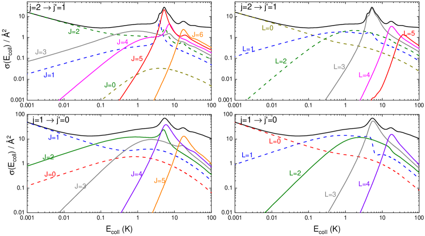
Figure 1: Total and partial integral cross sections for the H + HF($v$=0,$j$=1,2) inelastic collisions as a function of the collision energy. The total cross section for $j$=2 $\rightarrow$ $j^{\prime}$=1 (top panels) and $j$=1 $\rightarrow$ $j^{\prime}$=0 (bottom panels) are shown as solid black lines. The contributions of each $J$ (left panels) and $L$ (right panels) partial waves to the total cross section are also shown.

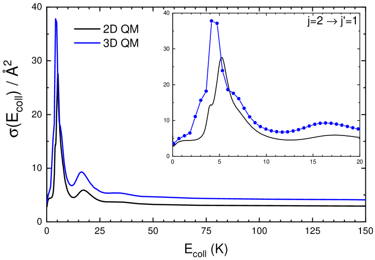
Figure S1: Comparison of 3D and 2D (fixed HF internuclear distance) quantum scattering calculation for $j=2\rightarrow j^{\prime}=1$. 2D calculations underestimate the cross section by 30% at the resonance peak, but capture all the features observed in the 3D cross section.

Since the aim of this work is i) the characterization of the observed resonances, and ii) to elucidate the extent of control that can be achieved, quantum mechanical (QM) scattering calculations were performed in a dense grid of collision energies starting at very low energies, $E_{\rm coll}/k_{\rm B}<$1 mK, and up to 100 K. To get an accurate description of the dynamics, it was necessary to propagate the wave-function up to very large distances ($6\cdot 10^{4}$ a₀), which made convenient to use the atom-rigid rotor approximation. Calculations were performed using the ASPIN code López-Durán et al. (2008); González-Sánchez et al. (2015) on the LWA-78 Potential Energy Surface, Li et al. (2007) which has been recently used to study H+HF collisions at higher energies.Desrousseaux and Lique (2018) To check the validity of the atom rigid-rotor approximation, full-dimensional QM scattering calculations were carried out for a few energies using the ABC code. Skouteris et al. (2000) The agreement between the two sets of calculations is good (see Fig. S1), although the atom-rigid rotor calculations underestimates the full-dimensional calculations at the highest energies by 20%. Both sets of calculations show the same overall behavior, and the main features of the full-dimensional results are well accounted for by the rigid-rotor calculations.

Figure 1 displays the energy dependence of the rotational quenching cross sections for HF($v$=0,$j$=1,2)+H collisions in the cold energy regime as function of the collision energy, $\sigma(E_{\rm coll})$, in the 1 mK–100 K $E_{\rm coll}$ range. Energies in this range are not sufficient to promote transitions to higher rotational states, and, besides, the probability for the H exchange channel is negligible.Desrousseaux and Lique (2018); Jambrina et al. (2019b) Hence, the only possible transitions are $j=1\rightarrow j^{\prime}=0$, and $j=2\rightarrow j^{\prime}=1$, 0. For a given $E_{\rm coll}$, $\sigma(E_{\rm coll})$ for $j=1\rightarrow j^{\prime}=0$ is 3-5 times higher than for $j=2\rightarrow j^{\prime}=1$ due to the wider gap between adjacent rotational quantum states with increasing $j$.Jambrina et al. (2019b) The Wigner regime for both channels is attained at energies below 5 mK, where $\sigma(E_{\rm coll})\propto E_{\rm coll}^{-1/2}$. Sadeghpour et al. (2000); Idziaszek et al. (2011) The respective $L$ partial cross sections, $\sigma^{L}(E_{\rm coll})$, and $J$-partial cross section, $\sigma^{J}(E_{\rm coll})$, are also shown in Fig. 1. As expected, at the Wigner regime only the s-wave ($L$=0, $J$=$j$) partial wave contributes significantly to the cross section. The corresponding Wigner limit, $\sigma^{L}\propto E_{\rm coll}^{L-1/2}$, is also found for $L>0$.Lara et al. (2015b)

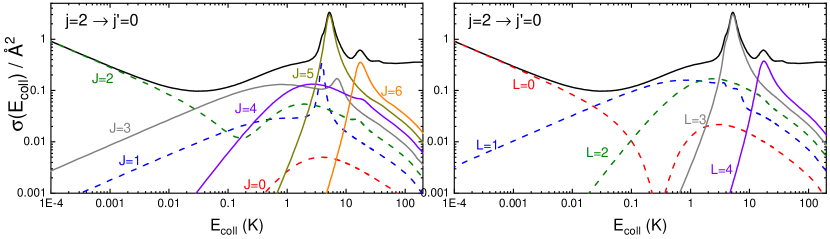
Figure S2: Total (black line), $L$-partial (right panel) and $J$-partial (left panel) integral cross sections for the $j=2\rightarrow j^{\prime}=0$ collision.

Most notably is that, at energies above the Wigner regime, $\sigma(E_{\rm coll})$ is dominated by a narrow peak located at around 5 K for the $j=2\rightarrow j^{\prime}=1$ transition and around 5.5 K for the $j=1\rightarrow j^{\prime}=0$ transition. At significantly higher energies, $E_{\rm coll}\sim$ 17 K, a broader albeit smaller peak shows up. Results for $j=2\rightarrow j^{\prime}=0$ are shown in Fig. S2, and although $\sigma(E_{\rm coll})$ is smaller by at least one order of magnitude, it features the same resonance peaks as $j=2\rightarrow j^{\prime}=1$. From inspection of $\sigma^{L}(E_{\rm coll})$, it is clear that the sharp resonance peak at 5 mK is exclusively due to $L$=3 and that the second broader peak can be mainly attributed to $L$=4. Nevertheless, the analysis of $\sigma^{J}(E_{\rm coll})$ shows that each peak can be decomposed in a series of maxima corresponding to different $J$s and the same $L$.

A further analysis can be carried out by plotting the contributions from the different $J$ to a given $L$, the double partial cross sections $\sigma^{L,J}(E_{\rm coll})$, as shown in Fig. 2 for $L$=3 near the resonance. For $j=2\rightarrow j^{\prime}=1$, $J=1-5$ contribute to $L$=3 ($L-j\leq J\leq L+j$), and their respective $\sigma^{L=3,J}(E_{\rm coll})$ show maxima that are shifted in a relatively broad range of $E_{\rm coll}$, as shown in Table 1. From these peaks, $J$=1 and 5 contribute the most to the overall intensity, while the contributions of $J$=2 and 3 are almost negligible. The shifting of the maxima for $J$=1 and 5 leads to the small shoulder observed in the overall resonance peak. For the $j=1\rightarrow j^{\prime}=0$ transition, only $J=$2 and mainly $J$=4 contribute to $L$=3 (due to the parity conservation). In this case, the position of the maxima is very similar and hence there are no shoulders in the overall $\sigma(E_{\rm coll})$.

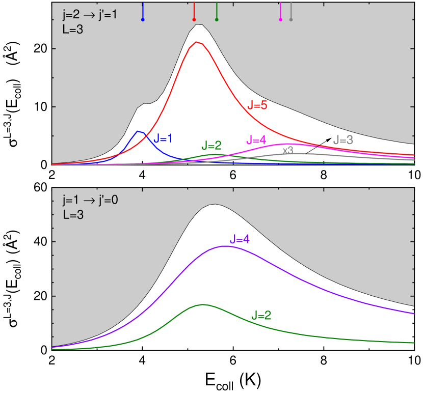
Figure 2: $L$=3 partial cross sections for $j=2\rightarrow j^{\prime}=1$ (top panel) and $j=1\rightarrow j^{\prime}=0$ (bottom panel). The white area correspond to the total cross section for $L$=3, $\sigma^{L=3}(E_{\rm coll})$, while the solid lines indicate the contribution of each $J$, $\sigma^{L,J}(E_{\rm coll})$. The positions of the resonance peaks predicted by the 1D-model are shown as solid vertical lines.

To characterize the nature of the aforementioned resonances, 1D adiabatic effective potentials for different rovibrational states have been calculated as a function of the atom-diatom distance (see supplementary information for further details). Two of them are shown in Fig 3. The binding character at short distances and the centrifugal barrier are evident in the figure. By tunneling, the trapping region is accessible, supporting quasibound states that give rise to shape resonances. The energies at which the 1D model predicts the peaks of each ($L$,$J$) resonance are shown in Table 1, and in Fig. 2 as vertical ticks. As can be observed, the agreement between the energies of the resonances and the maxima of the peaks is almost perfect, allowing us to attribute these peaks to shape resonances arising from different combinations of $J$ and $L$. The lifetimes and line shapes associated with each resonance were also calculated using the 1D model (Fig. 4), and the scattering probabilities. The results are compared in Table 1 showing that the lifetimes obtained with the two methods are in good agreement, with the 1D model predicting slightly longer lifetimes. The lifetimes for the $L$=3 resonances are significantly longer, revealing that $L$=3 and $L$=4 resonances have a different character.

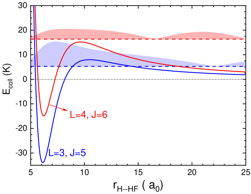
Figure 3: One-dimensional adiabatic effective intermolecular potential as a function of the distance between H and the center-of-mass of HF for two combinations of $J$ and $L$ of the $j=2\rightarrow j^{\prime}=1$ transition. The energies corresponding to the maximum time delay associated with these potentials are shown as dashed lines, along with the continuum wavefunctions. The shaded area is proportional to the square of the wavefunction.

$L$=3
$J$	$E$ (K)	$\tau$ (ps)	$E$ (K) 1D	$\tau$ (ps) 1D
1	3.9	11.3	4.0	14.0
2	5.5	4.4	5.6	5.2
3	7.1	2.4	7.3	2.6
4	7.0	2.6	7.0	2.8
5	5.1	4.9	5.1	6.8
$L$=4
6	16.2	0.90	16.3	1.0

Table 1: Energy ($E_{\rm coll}$) and lifetimes, $\tau$, of each of the manifold of resonances for $L$=3 and $L$=4 of the $j=2\rightarrow j^{\prime}=1$ transition. The second and third columns are, respectively, the energies of the resonance peaks and the lifetimes obtained form the Lorentzian profiles of the collision probabilities after substraction of the scattering background. The fourth and fifth columns are the respective data obtained by applying the 1D model described in the Supplementary information.

To further clarify the origin of the differences in the lifetimes of the various $J,L$ resonances, the effective adiabatic 1D potentials for the $L$=3–$J$=5 and $L$=4–$J$=6 particular cases are shown in Fig. 3. Along with the potentials, we show the energy of the quasibound states supported by these potentials (dashed lines) and the corresponding squares of the wavefunctions. For the $L$=3 peak, the energy of the quasi-bound state lies below the maximum of the centrifugal barrier, and it can be properly considered as a shape resonance. However, for the $L$=4 peak, the resonance energy lies slightly above the maximum of the barrier. As a consequence, the probability is more evenly spread over all radial distances, and the resonance exhibits a smaller lifetime. This kind of resonance can thus be characterized as an over-barrier (or “above-the-barrier”) resonance, the quantum equivalent to classical-orbiting Paliwal et al. (2020).

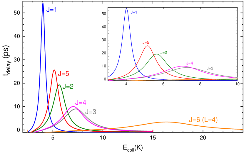
Figure 4: $t_{delay}(E)$ as a function of the collision energy for $L$=3 manifold of resonances for $j=2\rightarrow j^{\prime}=1$ transition. $t_{delay}(E)$ for $L$=4 and $J$=6 is also shown for the sake of comparison. The insert shows a blow-up of the energy range where the $L=3$ resonances show up.

In Ref. 14 it was found that the strength of the resonance peak can be tuned by alignment of rotational angular momentum and hence by changing the internuclear axis distribution. To check if it is also the case for H+HF collisions, we have used the procedure outlined in Refs. 39; 40; 41; 42 to investigate how the integral cross sections change by varying the angle $\beta$ between the polarization vector of the radiation field, used to prepare the HF molecule in specific rovibrational states, and the initial relative velocity vector. Each $\beta$ value entails a distribution of internuclear axis: if $\beta$=0^∘ collisions are preferentially head-on, while $\beta$=90^∘ implies a side-on geometry. The respective cross sections will be denoted by $\sigma^{\beta}(E_{\rm coll})$. These preparations can be contrasted with the “isotropic” distribution, with no external alignment.

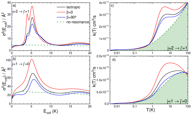
Figure 5: Left panels: cross-sections for different preparations of HF internuclear axis, $\beta$=0^∘ (red line) and $\beta$=90^∘ (blue line). The isotropic preparation (absence of external alignment) is shown in black. The dashed lines correspond to the background cross section when the resonance has been removed. Results for $j=2\rightarrow j^{\prime}=1$ and $j=1\rightarrow j^{\prime}=0$ are shown in panels (a) and (b), respectively. Right panels: Thermal rate coefficients (averaged over the MB distribution) for the mentioned transitions and internuclear axis preparations. The contribution of the background (no resonance) is shown shaded.

The left panels in Fig 5 display the cross sections for $j=2\rightarrow j^{\prime}=1$ (Fig. 5-a) and $j=1\rightarrow j^{\prime}=0$ (Fig. 5-b) in the vicinity of the $L$=3 resonance for isotropic distribution, $\beta$=0^∘ and $\beta$=90^∘. For $j=2\rightarrow j^{\prime}=1$ (a) the $L$=3 resonance is significantly enhanced for head-on ($\beta$=0^∘) encounters while its intensity decreases for side-on encounters. Outside the resonance region, the effect of a preferential alignment is unimportant. The most interesting feature is that the $\beta$=0 alignment is able to disentangle the peaks for $J$=1 and $J$=5; the contribution of $J$=1, which in the isotropic case manifests as a shoulder in the $L$=3 resonance, is enhanced to the point of splitting the original peak in two. Since $\beta$=0 implies collisions with $\Omega$=0 exclusively, where $\Omega$ is the projection of the total angular momentum vector onto the relative velocity, this implies that the $J$=1 partial wave has a strong component of the perpendicular projection. For $j=1\rightarrow j^{\prime}=0$ (Fig. 5-b) the cross-section is also enhanced for $\beta$=0, and this effect is particularly prominent at the resonance. In addition, the preference for head-on collisions is observed in a broad range of $E_{\rm coll}$. In this case, the resonance peak does not split for any HF preparation, as the energies corresponding to the two shape resonances contributing to this peak are very similar. These results for both transitions evince that the trapping of the collision complex is more efficient for head-on collisions.

Figures 5 c-d show the thermal rate coefficients, $k(T)$, calculated for the two transitions averaged over the Maxwell-Boltzmann distribution. In general, it is not guaranteed that a resonance may influence the rate coefficients significantly. However, in the present case, the resonance has a strong effect on $k(T)$ in the 1-50 K temperature range, leading to more than a two-fold increase of $k(T)$ for $j$=2 $\rightarrow$ $j^{\prime}$=1 at 5 K. The different intermolecular axis preparations also have a strong effect on the $k(T)$ in the same temperature range, with $\beta=0$ encounters leading to the largest $k(T)$. It also worth noticing that, while for $j$=2 $\rightarrow$ $j^{\prime}$=1 the $k(T)$ calculated with the resonance artificially removed rises monotonically with $T$, for $j$=1 $\rightarrow$ $j^{\prime}$=0 it starts decreasing at 40 K, effect that is even more clear for $\beta$=0.

In summary, in this study we have demonstrated that H + HF inelastic collisions in the 1-10 K ($E_{\rm coll}/k_{\rm B}$) energy range are dominated by shape resonances, which are themselves formed by a cluster of resonances, each of them characterized by orbital and total angular momentum values. We have shown that a 1-D model, based on the adiabatic effective potentials, can predict the position of the each $L$-$J$ resonance very accurately. Lifetimes and line-shapes of each of the resonances were determined using the phase-shift of the 1D continuum wavefunctions. In particular, the $L$=4 resonances exhibit shorter lifetimes and can be considered orbiting (over-the-barrier) resonances where the quasi-bound states lie slightly above the centrifugal barrier. In spite of the relatively large time delays associated to the resonances, alignment of HF prior the collision changes significantly both the intensity and shape of the excitation functions, which also manifest in the thermal rate coefficients. Remarkably, for $j=2\rightarrow j^{\prime}=1$, when head-on collisions are promoted, the main resonance peak splits in two, each of them associated to collisions with a particular value of the total angular momentum. These results are in contrast to those found for HD + H₂ collisions in the cold energy regime, for which the resonance vanishes for head-on encounters, showing that the degree of control associated to the resonance is very sensitive of the topology of the system. The influence of the resonance persists after the energy averaging and it leads to up to two-fold increase of the thermal rate coefficient at relevant temperatures of the interstellar medium where HF is ubiquitous.

The authors thank Prof. Enrique Verdasco for his support and help with the calculations. Funding by the Spanish Ministry of Science and Innovation (grant and PGC2018-096444-B-I00) is also acknowledged. P.G.J. acknowledges funding by Fundación Salamanca City of Culture and Knowledge (programme for attracting scientific talent to Salamanca).

I Supplementary Material

I.1 Scattering calculations:

The usual time-independent formulation of the coupled channel (CC) method is used to solve the Schrödinger equation, in the quantum scattering calculations of an atom with a diatomic molecule, as implemented in ASPIN code.López-Durán et al. (2008) The HF molecule in its singlet ground state is treated as a rigid rotor, while the H atom is considered structureless. Details of the method have been given before and discussed recently in detail for the case of the Rb + OD^-/OH^- system González-Sánchez et al. (2015) and will not be reported here. The parameters used for applying the CC method are chosen for achieving numerical convergence of the final S-matrix elements. A maximum number of rotational channels up to $j_{max}$ = 10 has been included in each CC calculation, where at least five channels were included as closed channels for each collision energy, ensuring overall convergence of the inelastic cross sections. At the lowest considered collision energies the radial integration was extended out to $R_{max}$ =$5\cdot 10^{4}$ Å.

To check the validity of the rigid rotor approximations, full-dimensional QM calculations were also obtained using the ABC code. Skouteris et al. (2000) Calculations were carried out for 80 energies, up to 150 K, including all partial waves to convergence. The propagation was carried out in 2000 log-derivative steps up to a hyperradius of 40 a₀. The basis included all the accessible states up to $E$=3.0 eV.

I.2 Partial cross sections

The expression of the probability for the $j\to j^{\prime}$ transition and for given total, $J$, and orbital, $L$, angular momentum values can be written as:

$$P_{j\to j^{\prime}}(J,L)=\sum_{L^{\prime}}\sum_{\epsilon}|S_{v^{\prime},j^{\prime}L^{\prime}\,\,v,j,L}^{J{\rm\epsilon}}|^{2},$$ (1)

where $S_{v^{\prime},j^{\prime}L^{\prime}\,\,v,j,L}^{J{\rm\epsilon}}$ is the scattering matrix element for the process between the reactant channel $(v,j,L)$ and the product channel $(v^{\prime},j^{\prime},L^{\prime})$, for $J$ and the parity $\rm\epsilon=(-1)^{(j+L)}=(-1)^{(j^{\prime}+L^{\prime})}$. In Eq. (1), the sums run over the possible values of the final orbital angular momentum $L^{\prime}$, and the parity $\rm\epsilon$ .

for a given value of the collision energy, the double partial cross section is given by

$$\sigma^{J,L}_{j\to j^{\prime}}=\frac{\pi}{k^{2}}\,\frac{2J+1}{2j+1}P_{j\to j^{\prime}}(J,L)$$ (2)

If summed over $J$ one gets the $J$ partial cross section:

$$\sum_{J=|L-j|}^{L+j}\,\sigma^{J,L}_{j\to j^{\prime}}=\frac{\pi}{k^{2}}\,\sum_{J=|L-j|}^{L+j}\frac{2J+1}{2j+1}P_{j\to j^{\prime}}(J,L)=\sigma^{L}_{j\to j^{\prime}}$$ (3)

Alternatively, by summing over $L$, the $J$ partial cross section is retrieved:

$$\sum_{L=|J-j|}^{J+j}\,\sigma^{J,L}_{j\to j^{\prime}}=\frac{\pi}{k^{2}}\,\frac{2J+1}{2j+1}\sum_{L=|J-j|}^{J+j}P_{j\to j^{\prime}}(J,L)=\sigma^{J}_{j\to j^{\prime}}$$ (4)

I.3 1D-model:

To understand the nature of the peaks observed in the cross-sections, and confirm their resonant nature, we have used a simple, essentially elastic, one-dimensional model. It is based on the calculation of 1D adiabatic potentials, to describe the effective interaction felt by the diatom when it gets close to the H atom. It is convenient to use $(R,r,\gamma)$ Jacobi coordinates to describe the scattering process: $R$ is the distance between H and the centre-of-mass of HF, $r$ the HF internuclear distance (kept fixed in the rigid rotor approximation) and $\gamma$ the angle between $R$ and $r$. The potentials, which depend on the initial quantum numbers of the colliding partners, have been calculated by adiabatically separating $\gamma$ from $R$. For a given value of $R$, the matrix elements of all the terms in the rigid-rotor Hamiltonian, except for the radial collision kinetic energy, are calculated in a basis of reactant channels, labeled by the set of quantum numbers $(J,M,j,L)$ and the parity $\epsilon$. Only states with the same values of $J,M$ and $\epsilon$ are coupled. This way, we diagonalize the block matrix corresponding to each pair $(J,\epsilon)$ ($M$ being irrelevant) including as many different $j$s and $L$s as needed for convergence.Lara et al. (2012) The resulting potentials,each of them correlating with a particular set of initial quantum numbers, support quasibound states, whose energies lie very close to the observed peaks.

To predict the approximate position, $E_{0}$, and the width, $\Gamma$, of the resonances, we calculate the time-delay function, $t_{\rm delay}(E)$. The time-delay is (in our context) a measurement of the time that the internuclear complex is trapped in the potential well. It can be calculated from the phase-shift of the 1D continuum wavefunction using the expression: Child (1974); Goldberger and Watson (1992)

$$t_{\rm delay}(E)=2\hbar(d\phi/dE),$$ (5)

The time-delay functions provided by the 1D model are depicted in Fig.4. It is interesting to note their Lorentzian character. Indeed, in the absence of background, the time-delay has a pure Lorentzian line-shape centered precisely at $E_{0}$, Smith (1960, 1963)

$$t_{\rm delay}(E)=\hbar\Gamma/[(E-E_{0})^{2}+(\Gamma/2)^{2}]$$ (6)

where $\Gamma$ is the FWHM of the line-shape. Accordingly, $\Gamma$ and $t_{\rm delay}(E_{0})$ are related as:

$$t_{\rm delay}(E_{0})=\frac{4\hbar}{\Gamma},$$ (7)

Finally, the lifetime of the resonance (average time delay) is given by: Smith (1960)

$$\tau=\frac{\hbar}{\Gamma}=\frac{t_{\rm delay}(E_{0})}{4}.$$ (8)

These Eqs. would allow to calculate the features of a resonance starting from the time-delay functions in the absence of background scattering. However, in the presence of background scattering (as it is the case), we need to modify somewhat the fitting function. Assuming a background phase-shift which changes linearly with energy around $E_{0}$ ($\delta_{back}(E)=b+a(E-E_{0})$), the maximum of the total time-delay will still provide $E_{0}$. In turn, once $E_{0}$ is known, the width can be determined fitting the time-delay to the analytical expression:

$$t_{\rm delay}(E)=a+\hbar\Gamma/[(E-E_{0})^{2}+(\Gamma/2)^{2}]$$ (9)

The resulting positions and widths predicted by the 1D model are shown in Table I of the main text. They have been compared with those extracted from the full scattering calculation. Assuming a contribution up to first order in $(E-E_{0})$ from the background scattering to the S-matrix elements,de Jongh et al. (2020) we have used the following function to fit the $L$-$J$ inelastic probabilities:

$$P(E)=P_{3}[(E-E_{0})]/[(E-E_{0})^{2}+(\Gamma/2)^{2}]$$ (10)

where $P_{3}[(E-E_{0})]$ is a third degree polynomial in the variable $(E-E_{0})$, whose unknown coefficients are also given by the fitting process.

Let us finally note that, as can be easily conclude from the data in Table I, the lifetimes provided by the 1D-model are an upper bound to the full-scattering ones. Indeed, the adiabatic Hamiltonian suppresses the kinetic couplings between different adiabatic curves. A resonance supported by one of this curves, can only decay by tunneling through the centrifugal barrier. However, under the exact Hamiltonian, resonances are coupled to other adiabatic states; hence there is an alternative mechanism of decay, which is expected to disminish the lifetime.

I.4 Alignment-dependent cross sections:

Let us define a scattering frame with the $z$ axis along the initial relative velocity and the $xz$ plane as the one determined by the initial and final relative velocities. Let us note with $\beta$ the polar angle that specifies the direction of the polarization vector in the scattering frame. Following Ref. 41, the cross sections for a given $\beta$, is given by:

$$\sigma^{\beta}=\sigma_{\rm iso}\sum_{k}^{2j}(2k+1)s^{(k)}_{0}P_{k}(\cos\beta)A^{(k)}_{0}$$ (11)

where $\sigma_{\rm iso}$ is the unpolarized cross section, $P_{k}(\cos\beta)$ are the Legendre polynomials, and $s^{(k)}_{0}$ and $A^{(k)}_{0}$ are the intrinsic and extrinsic polarization parameters. The latter is a geometrical factor that, for optical pumping, is given by the $\langle j0,k0|j0\rangle$ Clebsch-Gordan coefficient. The $s^{(k)}_{0}$ polarization parameters can be calculated from the S-matrix as: Aldegunde et al. (2012)

$$s^{(k)}_{0}=\frac{\pi}{\sigma_{\rm iso}\,k^{2}}\,\,\sum_{J}\sum_{\Omega^{\prime},\Omega}(2J+1)|S^{J}_{j^{\prime},\Omega^{\prime},j,\Omega}|^{2}\langle j\Omega,k0|j\Omega\rangle$$ (12)

where $\Omega$ and $\Omega^{\prime}$ are the helicities, i.e., the projections of $J$ on the directions of the reactant’s approach and the product’s recoil, respectively. $\beta$=0^∘ (which is equivalent to $\Omega=0$) collisions are preferentially head-on, while $\beta$=90^∘ implies side-on encounters.

The values of $\sigma^{\beta}$ ($\beta=0^{\circ},\beta=90^{\circ}$) relative to $\sigma_{\rm iso}$ are shown in Fig. S3 for the three transitions considered in this work, and in a wide range of collision energies. At the lowest energies, close to the Wigner limit, $\sigma^{\beta}$ is independent on the preparation. Aldegunde et al. (2006); Jambrina et al. (2019a) In the vicinity of the resonance, head-on collisions prevail while at energies above 200 K side-on arrangements lead to higher cross sections. The preponderance of the $\beta=0^{\circ}$ preparation in the cold regime for the $j=1,2\rightarrow j^{\prime}=0$ transitions (upper panels of Fig. S3) stems from the fact that for $j^{\prime}=$0 there is only one possible parity, $(-1)^{J}$, which includes $\Omega=0$, and hence the weight of this projection is higher than that when the two parities contribute to scattering (the $(-1)^{J+1}$ parity does not include $\Omega$=0), as is the case for the $j=2\rightarrow j^{\prime}=1$ transition. At energies above the 100-300 K side-on collisions are preferred, as expected from classical arguments.

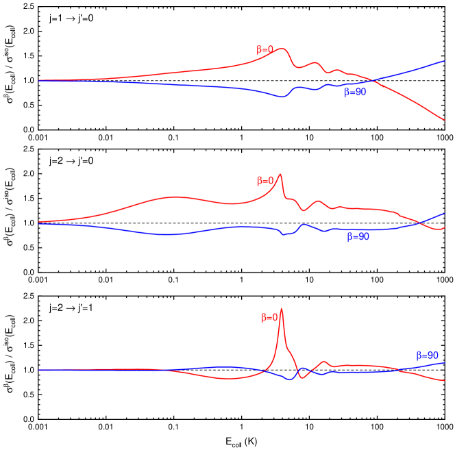
Figure S3: Ratio between the $\sigma(E)$ obtained for $\beta$=0, and $\beta$=90^∘ and the isotropic $\sigma(E)$. Results for the three opened states are shown.

References

- Liu (2012) K. Liu, Adv. Chem. Phys. 149, 1 (2012).
- Neumark et al. (1985) D. M. Neumark, A. M. Wodtke, G. N. Robinson, C. C. Hayden, and Y. T. Lee, J. Chem. Phys. 82, 3045 (1985).
- Vogels et al. (2015) S. N. Vogels, J. Onvlee, S. Chefdeville, A. van der Avoird, G. C. Groenenboom, and S. Y. T. van de Meerakker, Science 350, 787 (2015).
- de Jongh et al. (2020) T. de Jongh, M. Besemer, Q. Shuai, T. Karman, A. van der Avoird, G. C. Groenenboom, and S. Y. T. van de Meerakker, Science 368, 626 (2020).
- Paliwal et al. (2020) P. Paliwal, N. Deb, D. M. Reich, C. P. Koch, and E. Narevicius, (2020), arXiv:2002.10750 [physics.chem-ph] .
- Bulut et al. (2015) N. Bulut, J. F. Castillo, P. G. Jambrina, J. Klos, O. Roncero, F. J. Aoiz, and L. Banares, J. Phys. Chem. A 119, 11951 (2015).
- Jambrina et al. (2010) P. G. Jambrina, F. J. Aoiz, N. Bulut, S. C. Smith, G. G. Balint-Kurti, and M. Hankel, Phys. Chem. Chem. Phys. 12, 1102 (2010).
- Lara et al. (2015a) M. Lara, P. G. Jambrina, F. J. Aoiz, and J. M. Launay, J. Chem. Phys. 143, 204305 (2015a).
- Bonnet and Larregaray (2020) L. Bonnet and P. Larregaray, J. Chem. Phys. 152, 084117 (2020).
- Perreault et al. (2017) W. E. Perreault, N. Mukherjee, and R. N. Zare, Science 358, 356 (2017).
- Perreault et al. (2018) W. E. Perreault, N. Mukherjee, and R. N. Zare, Nat. Chem. 10, 561 (2018).
- Croft et al. (2018) J. F. E. Croft, N. Balakrishnan, M. Huang, and H. Guo, Phys. Rev. Lett. 121, 113401 (2018).
- Croft and Balakrishnan (2019) J. F. E. Croft and N. Balakrishnan, J. Chem. Phys. 150, 164302 (2019).
- Jambrina et al. (2019a) P. G. Jambrina, J. F. E. Croft, H. Guo, M. Brouard, N. Balakrishnan, and F. J. Aoiz, Phys. Rev. Lett. 123, 043401 (2019a).
- Skodje et al. (2000) R. T. Skodje, D. Skouteris, D. E. Manolopoulos, S.-H. Lee, F. Dong, and K. Liu, Phys. Rev. Lett. 85, 1206 (2000).
- Qiu et al. (2006) M. Qiu, Z. Ren, L. Che, D. Dai, S. A. Harich, X. Wang, X. Yang, C. Xu, D. Xie, M. Gustafsson, R. T. Skodje, Z. Sun, and D. H. Zhang, Science 311, 1440 (2006).
- Dong et al. (2010) W. Dong, C. Xiao, T. Wang, D. Dai, X. Yang, and D. Zhang, Science 327, 1501 (2010).
- Wang et al. (2013) T. Wang, J. Chen, T. Yang, C. Xiao, Z. Sun, L. Huang, D. Dai, X. Yang, and D. Zhang, Science 342, 1499 (2013).
- Kim et al. (2015) J. Kim, M. Weichman, T. Sjolander, D. Neumark, J. Klos, M. Alexander, and D. Manolopoulos, Science 349, 510 (2015).
- Yang et al. (2019) T. Yang, L. Huang, C. Xiao, J. Chen, T. Wang, D. Dai, F. Lique, M. H. Alexander, Z. Sun, D. H. Zhang, X. Yang, and D. M. Neumark, Nat. Chem. 11, 744 (2019).
- Manolopoulos (1997) D. E. Manolopoulos, J. Chem. Soc. Faraday Trans. 93, 673 (1997).
- Alexander et al. (2000) M. H. Alexander, D. E. Manolopoulos, and H. J. Werner, J. Chem. Phys. 113, 11084 (2000).
- Lique et al. (2008) F. Lique, M. H. Alexander, G. Li, H. J. Werner, S. A. Nizkorodov, W. W. Harper, and D. J. Nesbitt, J. Chem. Phys. 128, 084313 (2008).
- Aldegunde et al. (2011) J. Aldegunde, P. G. Jambrina, M. P. De Miranda, V. Sáez-Rábanos, and F. J. Aoiz, Phys. Chem. Chem. Phys. 13, 8345 (2011).
- Tizniti et al. (2014) M. Tizniti, S. Le Picard, F. Lique, C. Berteloite, A. Canosa, M. H. Alexander, and I. R. Sims, Nat. Chem. 6, 141 (2014).
- Sáez-Rábanos et al. (2019) V. Sáez-Rábanos, J. E. Verdasco, and V. J. Herrero, Phys. Chem. Chem. Phys. 21, 15177 (2019).
- De Fazio et al. (2020) D. De Fazio, V. Aquilanti, and S. Cavalli, J. Phys. Chem. A 124, 12 (2020).
- Agúndez, M. et al. (2011) Agúndez, M., Cernicharo, J., Waters, L. B. F. M., Decin, L., Encrenaz, P., Neufeld, D., Teyssier, D., and Daniel, F., A&A 533, L6 (2011).
- Indriolo et al. (2013) N. Indriolo, D. A. Neufeld, A. Seifahrt, and M. J. Richter, Astrophys. J. 764, 188 (2013).
- Desrousseaux and Lique (2018) B. Desrousseaux and F. Lique, Mon. Not. R. Astron. Soc. 476, 4179 (2018).
- López-Durán et al. (2008) D. López-Durán, E. Bodo, and F. Gianturco, Computer Phys. Comm. 179, 821 (2008).
- González-Sánchez et al. (2015) L. González-Sánchez, F. A. Gianturco, F. Carelli, and R. Wester, New J. Phys. 17, 123003 (2015).
- Li et al. (2007) G. Li, H.-J. Werner, F. Lique, and M. H. Alexander, J. Chem. Phys. 127, 174302 (2007).
- Skouteris et al. (2000) D. Skouteris, J. F. Castillo, and D. E. Manolopoulos, Comp. Phys. Comm. 133, 128 (2000).
- Jambrina et al. (2019b) P. G. Jambrina, L. González-Sánchez, J. Aldegunde, V. Sáez-Rábanos, and F. J. Aoiz, J. Phys. Chem. A 123, 9079 (2019b).
- Sadeghpour et al. (2000) H. R. Sadeghpour, J. L. Bohn, M. J. Cavagnero, B. D. Esry, I. I. Fabrikant, J. H. Macek, and A. R. P. Rau, J. Phys. B 33, R93 (2000).
- Idziaszek et al. (2011) Z. Idziaszek, A. Simoni, T. Calarco, and P. S. Julienne, New J. Phys. 13, 083005 (2011).
- Lara et al. (2015b) M. Lara, P. G. Jambrina, J. M. Launay, and F. J. Aoiz, Phys. Rev A 91, 030701R (2015b).
- Aoiz and de Miranda (2010) F. J. Aoiz and M. P. de Miranda, in Tutorials in Molecular Reaction Dynamics, edited by M. Brouard and C. Vallance (RSC Publishing, 2010).
- Case and Herschbach (1975) D. A. Case and D. R. Herschbach, Mol. Phys. 30, 1537 (1975).
- Aldegunde et al. (2005) J. Aldegunde, M. P. de Miranda, J. M. Haigh, B. K. Kendrick, V. Saez-Rabanos, and F. J. Aoiz, J. Phys. Chem. A 109, 6200 (2005).
- Aldegunde et al. (2012) J. Aldegunde, D. Herraez-Aguilar, P. G. Jambrina, F. J. Aoiz, J. Jankunas, and R. N. Zare, J. Phys. Chem. Lett. 3, 2959 (2012).
- Lara et al. (2012) M. Lara, S. Chefdeville, K. M. Hickson, A. Bergeat, C. Naulin, J.-M. Launay, and M. Costes, Phys. Rev. Lett. 109, 133201 (2012).
- Child (1974) M. S. Child, Molecular Collision Theory (Academic Press, Republished by Dover 1996, 1974).
- Goldberger and Watson (1992) M. L. Goldberger and K. M. Watson, Collision Theory (John Wiley and Sons, Inc., Republished by Dover 2004, 1992).
- Smith (1960) F. T. Smith, Phys. Rev. 118, 349 (1960).
- Smith (1963) F. T. Smith, Phys. Rev. 130, 394 (1963).
- Aldegunde et al. (2006) J. Aldegunde, J. M. Alvariño, M. P. de Miranda, V. Sáez-Rábanos, and F. J. Aoiz, J. Chem. Phys. 125, 133104 (2006).