Efficient Approximation Schemes for
Stochastic Probing and Prophet Problems

Our main contribution is a general framework to design efficient polynomial time approximation schemes (EPTAS) for fundamental stochastic combinatorial optimization problems. Given an error parameter $\epsilon>0$, such algorithmic schemes attain a $(1-\epsilon)$-approximation in $t(\epsilon)\cdot\operatorname{poly}(n)$ time, where $t(\cdot)$ is some function that depends only on $\epsilon$. Technically speaking, our approach relies on presenting tailor-made reductions to a newly-introduced multi-dimensional load balancing problem. Even though the single-dimensional problem is already known to be APX-Hard, we prove that an EPTAS can be designed under certain structural assumptions, which hold for each of our applications.

To demonstrate the versatility of our framework, we first study selection-stopping settings to derive an EPTAS for the Free-Order Prophets problem [Agrawal et al., EC’20] and for its cost-driven generalization, Pandora’s Box with Commitment [Fu et al., ICALP’18]. These results constitute the first approximation schemes in the non-adaptive setting and improve on known inefficient polynomial time approximation schemes (PTAS) for their adaptive variants. Next, turning our attention to stochastic probing problems, we obtain an EPTAS for the adaptive ProbeMax problem as well as for its non-adaptive counterpart; in both cases, state-of-the-art approximability results have been inefficient PTASes [Chen et al., NIPS’16; Fu et al., ICALP’18].

1 Introduction

The field of combinatorial optimization typically deals with computational problems where we are given an objective function $f:2^{[n]}\rightarrow\mathbb{R}$ on $n$ elements along with certain feasibility constraints $\mathcal{F}\subseteq 2^{[n]}$; our goal is to find in polynomial time a set $S\in\mathcal{F}$ that maximizes $f(S)$, potentially in an approximate way. In the last two decades, there has been a great deal of interest in studying combinatorial optimization problems under various notions of uncertainty. In particular, a frequent meta-question in this context is: Can we handle objective functions that involve random variables, when our algorithm only has access to their probability distributions?

For concreteness, consider an interviewing scenario where a firm wishes to hire one of $n$ candidates. This setting corresponds to the simplest non-trivial feasibility set $\mathcal{F}=\{\{i\}\mid i\in[n]\}$. Clearly, without any randomness the problem is trivial, as we can hire the highest value candidate. Now, suppose the value of each candidate $i$ is represented by a non-negative random variable $X_{i}$ drawn independently from some known element-dependent distribution. If we can only afford conducting $k<n$ interviews, which candidates should be interviewed? Formally, in the ProbeMax problem we probe a set $S\subseteq[n]$ of size at most $k$, with the goal of maximizing the expected highest probed value, i.e., ${\mathbb{E}}[\max_{i\in S}X_{i}]$. Interestingly, due to the specific nature of randomness, this problem can be defined in two ways depending on whether the algorithm probes the set $S$ adaptively or non-adaptively. Here, by “adaptively” we mean that the required algorithm is a policy (decision tree) that sequentially decides on the next element to be probed depending on the outcomes observed up until then. In contrast, a non-adaptive algorithm would decide on the set of elements to be probed a-priori, without observing any outcomes. Surprisingly, even for this seemingly-simple problem, finding the optimal non-adaptive solution is known to be NP-hard [CHL⁺16, GGM10] and it is believed that finding the optimal adaptive policy is #P (or even PSPACE) hard [FLX18]. As such, the natural question is: Can we efficiently find near-optimal adaptive and non-adaptive solutions?

As another motivating example, consider again an interviewing scenario where you may interview all candidates, but have to immediately decide upon interviewing whether to hire or reject the current candidate. Formally, this setting corresponds to the Free-Order Prophets problem, where the value of each element $i\in[n]$ is again specified by an independent random variable $X_{i}$. The algorithm is required to find a permutation $\sigma\in S_{n}$ in which the outcomes $X_{\sigma(i)}$ will be observed, and a stopping time $\tau$ to maximize the expected value of $X_{\tau}$. Due to a fundamental result of Hill [Hil83], it is known that there exists an optimal adaptive policy for this problem which is in fact non-adaptive, and we can therefore assume that the optimal permutation $\sigma^{*}$ is chosen a-priori. It is worth mentioning that, given a permutation, the optimal stopping time can easily be computed by dynamic programming (see further details in §3). However, finding the optimal permutation has very recently been proven by Agrawal et al. [ASZ20] to be NP-hard. In this context, the basic question is whether one can still obtain a non-trivial approximation.

Besides the above-mentioned probing and prophets problems, numerous additional stochastic optimization problems have previously been considered, such as variants of Pandora’s Box, Stochastic Matchings, and Stochastic Knapsack. Indeed, to date, constant factor approximations were attained for each of these problems, and we refer the reader to further discussion on related work in §1.3. This current state of knowledge raises the following question which motivates our work:

Can we find in polynomial time near-optimal solutions to adaptive and non-adaptive stochastic combinatorial optimization problems?

1.1 Our results

The main contribution of our work is a general approach to design efficient polynomial time approximation schemes (EPTAS) for a number of stochastic combinatorial optimization problems. That is, for any constant $\epsilon>0$, we obtain a $(1-\epsilon)$-approximation to the optimal objective value in $t(\epsilon)\cdot\operatorname{poly}(n)$ time, where $t(\cdot)$ is some function that depends only on $\epsilon$. For ease of presentation, we first discuss the algorithmic implications of our framework, which will be followed by its high-level technical ideas in §1.2.

Free-Order Prophets. This problem was first studied in the 1980’s by Hill [Hil83], who proved the existence of a non-adaptive optimal policy. From an algorithmic perspective, an approximation ratio of $1/2$ directly follows from the classical Prophet inequality [KS77, KS78, SC84], which provides a threshold-based algorithm with value at least $\frac{1}{2}\cdot\mathbb{E}[\max_{i}X_{i}]$. In a recent work, Agrawal et al. [ASZ20] obtained improved constant-factor approximations for special classes of distributions, such as when each random variable has a support size of at most two. However, prior to our work, existing approaches lose at least a constant factor in their guaranteed approximation ratio for arbitrary distributions. As a first demonstration of the applicability of our framework, we provide in §3 an EPTAS for this problem.

We remark that Fu et al. [FLX18] obtained an adaptive PTAS for the Pandora’s Box with Commitment problem, which captures Free-Order Prophets for zero costs. However, this result does not translate to a non-adaptive PTAS for finding a fixed permutation a-priori, and certainly not to an EPTAS.

ProbeMax. The first non-trivial results for ProbeMax and for additional Stochastic Probing problems were based on adaptivity-gap bounds. Such findings show that, up to certain constant factors, the adaptive and non-adaptive variants are equivalent in terms of approximability [AN16, GN13, GNS17]. Thus, specifically for ProbeMax, one can just focus on the non-adaptive problem, $\max_{S:|S|\leq k}\mathbb{E}[\max_{i\in S}X_{i}]$, which is a monotone submodular maximization problem and can therefore be approximated in polynomial time [NWF78]. Improving on these early results, Chen et al. [CHL⁺16] designed a DP-based polynomial time approximation scheme (PTAS) for non-adaptive ProbeMax, where a $(1-\epsilon)$-approximation was attained in $n^{t(\epsilon)}$ time. It is important to emphasize that this finding does not translate to a PTAS for adaptive ProbeMax, due to a constant factor gap between adaptive and non-adaptive settings. In a recent breakthrough work, Fu et al. [FLX18] devised a PTAS for the adaptive ProbeMax problem. Interestingly, their main idea is to design a policy that employs only constant rounds of adaptivity. Using our framework, we improve on the results of both Chen et al. [CHL⁺16] and Fu et al. [FLX18], showing that the ProbeMax problem actually admits an EPTAS (proved in §4 and §5, respectively).

It is worth pointing out that an EPTAS is particularly attractive from an implementation standpoint, due to ensuring that our running time dependency on the accuracy level $\epsilon$ is instance-independent. This property is very appealing to practitioners, who view running times such as $n^{1/\epsilon}$ as purely theoretical in certain settings, whereas terms of the form $(1/\epsilon)^{1/\epsilon}$ are more acceptable. In such practical settings, one would never fix $\epsilon=10^{-6}$, but even $\epsilon=0.1$ becomes impractical with $n^{1/\epsilon}$. For further discussion on EPTASes, we refer the avid reader to a number of selected papers in this context [HL04, Jan10, FLRS11, BBB⁺21].

Additionally, we note that even though the adaptive ProbeMax problem appears to be more “difficult” than its non-adaptive counterpart, we are not aware of any way to derive Theorem 1.2 as a corollary of Theorem 1.3. In essence, there is no natural way to transform a given decision tree into a non-adaptive solution while preserving its performance guarantee.

Extensions. In §6.1 we obtain an EPTAS for a variant of the classical Pandora’s Box problem [Wei79]. In Pandora’s Box with Commitment, introduced by Fu et al. [FLX18], one has to immediately decide upon observing a random variable whether to select it or not. Formally, given distributions of $n$ independent random variables $X_{1},\ldots,X_{n}$, the outcome of each $X_{i}$ can be observed by paying a known cost $c_{i}$; the algorithm is required to find a permutation $\sigma\in S_{n}$ to discover the outcomes and a stopping time $\tau$, so as to maximize $\mathbb{E}[X_{\sigma(\tau)}-\sum_{i\leq\tau}c_{\sigma(i)}]$. Fu et al. [FLX18] proposed an adaptive PTAS for this problem. Our contribution in this context is to prove that Pandora’s Box with Commitment is in fact equivalent to the Free-Order Prophets problem. More specifically, we show that the optimal solution to the former problem is a non-adaptive permutation, and that an $\alpha$-approximation for Free-Order Prophets implies an $\alpha$-approximation for Pandora’s Box with Commitment. By combining this equivalence with Theorem 1.1, we derive the following result.

Finally, we show that our framework can be leveraged to obtain analogous results for broader settings, with multiple-element selection. In particular, in §6.2 we obtain an EPTAS for a generalization of non-adaptive ProbeMax where the algorithm has to non-adaptively select $k$ random variables, and its goal is to maximize the expected sum of the top $r$ selected variables.

1.2 High-level technical overview

Our approach to all stochastic optimization problems in question consists of presenting tailor-made reductions to a Multi-Dimensional Santa Claus problem. In this setting, formally defined in §2, we are given $n$ jobs that should be assigned to $m$ machines, where each job $j\in[n]$ incurs a vector load of $\ell_{ij}\in\mathbb{R}_{+}^{D}$ on machine $i\in[m]$. We are additionally given vector coverage constraints $\mathbf{L}_{i}\in\mathbb{R}_{+}^{D}$ for each machine $i$, and the goal is to compute an assignment in which the total vector load on each machine is at least $\mathbf{L}_{i}$, when such an assignment exists. Even when $D=1$, this formulation captures the well-known Santa Claus problem [BS06], which has been notoriously difficult, admitting constant-factor approximations only for certain special cases; e.g., see [AKS17, CCK09, Fei08, BD05]. In §2 we prove that, for a constant number of machines $m$ and dimensions $D$, an EPTAS can be designed for problem instances that satisfy the so-called “$\rho$-feasibility” condition, up to slightly violating the coverage constraints; this technical condition will be sufficient for our approximation schemes.

At a high-level, our approach for each stochastic optimization problem begins by breaking, for purposes of analysis, the optimal (non-)adaptive solution into disjoint buckets of random variables, where within any given bucket the solution’s performance does not change by much (up to a $(1-\epsilon)$-factor). After guessing a number of “hyper-parameters” that characterize each bucket, our algorithm wishes to assign the underlying random variables to the buckets defined earlier. Intuitively, the goal of these hyper-parameters is to capture crucial structural features of the optimal solution within each bucket. This reduction results in an instance of the Multi-Dimensional Santa Claus problem where random variables can be thought of as jobs that should be assigned to machines corresponding to buckets, while simultaneously satisfying $D$ hyper-parameter constraints.

Given the generic approach described above, the main challenge resides in defining the right bucketing and hyper-parameters, which are problem-specific decisions. It is important to mention that, besides capturing structural features of optimal solutions, hyper-parameters are required to have an additive form over the assigned random variables, since machine loads are additive within the Multi-Dimensional Santa Claus problem. In §3 we apply this approach to the Free-Order Prophets problem, where the application is easier than in other cases, since we make use of only a single hyper-parameter (i.e., $D=1$). In §4 we present an application to non-adaptive ProbeMax, where Multi-Dimensional Santa Claus comes up in its single-machine form. Finally, in §5 we consider adaptive ProbeMax, where the full power of Multi-Dimensional Santa Claus will be needed.

Comparison to Fu et al. [FLX18]. Technically speaking, our bucketing-with-hyper-parameters approach shares some similarities with the block-adaptive-with-signatures approach of Fu et al. [FLX18]. There are, however, crucial differences. Firstly, they define a block as a subset of random variables over which adaptivity is not helpful (up to $1-\epsilon$ factor). Our notion of buckets is much more general, as it also applies for problems such as Free-Order Prophets, where the optimal solution is non-adaptive. Secondly, and more importantly, we define buckets and hyper-parameters in order to facilitate a reduction to the Multi-Dimensional Santa Claus problem. In contrast, Fu et al. guess the signature of each block very accurately (up to $1-\frac{1}{\operatorname{poly}(n)}$) and utilize a massive dynamic program. It is unclear whether an EPTAS can be obtained through such dynamic programs, since $\epsilon$-factor errors in signature-related guesses could translate to unbounded errors for the entire problem.

1.3 Further Related Work

Evidently, in the last two decades, there has been a massive and ever-growing body of work on both probing and stopping-time stochastic optimization problems. Therefore, we mention below only the most-relevant papers, and refer the readers to [Sin18a] and to the references therein.

Probing problems have become increasingly-popular in theoretical computer science, starting at the influential work of Dean et al. [DGV04], who studied the stochastic knapsack problem. Additional streams of literature emerged from subsequent papers related to stochastic matchings by Chen et al. [CIK⁺09], stochastic submodular maximization by Asadpour et al. [ANS08], and variants of Pandora’s box by Kleinberg et al. [KWW16] and Singla [Sin18b]. These efforts resulted in constant-factor approximation algorithms, either using implicit bounds on the adaptivity gap involved via LP (or multilinear) relaxations, or directly through explicit bounds. Further work in this context considered a wide range of problems, including knapsack [BGK11, Ma14], orienteering [GM09, GKNR12, BN14], packing integer programs [DGV05, CIK⁺09, BGL⁺12], submodular objectives [GN13, ASW14, GNS17, BSZ19], matchings [Ada11, BGL⁺12, BCN⁺15, AGM15, GKS19], and Pandora’s box models [GJSS19, BK19, GKS19, JLLS20, BFLL20, CGT⁺20], just to mention a few representative papers.

A concurrent research direction investigates combinatorial generalizations of the classic secretary [Dyn63] and prophet inequality [KS77, KS78] stopping-time problems, due to their applications in algorithmic mechanism design [BIKK08, Luc17]. For secretary problem generalizations, we refer the reader to [GS20], as the existing literature is somewhat less relevant to our current work. Hajiaghayi et al. [HKS07] proved a prophet inequality for uniform matroids, and Alaei [Ala14] obtained the optimal $1+O(1/\sqrt{r})$ prophet inequality. A number of additional papers along these lines considered matroids [CHMS10, Yan11, KW12, EHKS18], matchings [FSZ16, EFGT20], and arbitrary downward-closed constraints [Rub16, RS17].

It is worth mentioning that all papers listed above (except for [BGK11]) lose at least a constant factor in their guaranteed approximation ratio. In contrast, there are only a handful of results for obtaining near-optimal policies. From this perspective, Bhalgat et al. [BGK11] devised a PTAS for the stochastic knapsack problem, with a $(1+\epsilon)$-relaxation of its packing constraint. To our knowledge, this is where the idea of block-adaptive policies was first introduced (see §5), followed by refinements in [LY13, FLX18] for other probing problems. Some recent papers have also tried to obtain $(1+\epsilon)$-approximations for prophets [ANSS19, ASZ20].

After an initial draft of this paper was put up online, parallel independent works of Mehta et al. [MNPR20] and Liu et al. [LLP⁺20] have also appeared, obtaining an EPTAS for non-adaptive ProbeMax and for Free-Order Prophets, respectively. However, their techniques are very different from ours.

1.4 Future directions

In this work we design EPTAS for a number of fundamental stochastic combinatorial optimization problems. An immediate open question for future research is whether these problems admit a fully polynomial time approximation schemes (FPTAS). That is, for any constant $\epsilon>0$, can we obtain a $(1+\epsilon)$-approximation in $t(\epsilon)\cdot\operatorname{poly}(n)$ time, where $t(\epsilon)$ is some polynomial in $1/\epsilon$?

Another interesting direction is to obtain an EPTAS/FPTAS for multiple-element selection variants of the problems studied in this paper. In §6.2 we discuss how our framework can be leveraged when the goal is to maximize the sum of top-$r$ elements, i.e., a uniform matroid of rank $r$. It is worth investigating whether similar results can be obtained for more general matroids (e.g., laminar matroids [ANSS19]).

2 EPTAS for Multi-Dimensional Santa Claus

In this section we provide a mathematical formulation of the Multi-Dimensional Santa Claus problem that lies at the heart of our algorithmic approach. With a concrete formulation in place, we show that for a fixed number of machines and for a fixed number of dimensions, this problem admits an efficient polynomial-time approximation scheme with a slight feasibility violation, which will be sufficient for our purposes.

2.1 Problem description

We consider a feasibility formulation of the Multi-Dimensional Santa Claus problem. Instances of this problem consist of the following ingredients:

• We are given a set of $m$ unrelated machines. Each machine $i$ is associated with an upper bound of $k_{i}$ on the number of jobs it can be assigned and a $D$-dimensional vector $\mathbf{L}_{i}\in\mathbb{R}^{D}_{+}$ that specifies a lower bound on the load vector of this machine.

• We have a collection of $n$ jobs, each of which can be assigned to at most one machine. When job $j$ is assigned to machine $i$, we incur a $D$-dimensional load, specified by the vector $\ell_{ij}\in\mathbb{R}^{D}_{+}$.

With respect to such instances, a job-to-machine assignment is defined as a function that decides for each job to which machine it is assigned. By slightly expanding the conventional term, an assignment is allowed to leave out any given job. We say that an assignment is feasible when each machine $i$ is assigned at most $k_{i}$ jobs, accumulating an overall load of at least $\mathbf{L}_{i}$. Our objective is to compute a feasible assignment, or to report that the instance in question is infeasible.

Integer programming formulation. Moving forward, it will be instructive to express this problem via the integer program (IP), whose specifics are described below. For simplicity of notation, we assume without loss of generality that the lower bound $\mathbf{L}_{i}$ on the load of each machine $i$ is a 0/1-vector; this assumption can easily be enforced by scaling. As such, ${\cal A}_{i}$ will stand for the subset of dimensions where $\mathbf{L}_{i}$ is active, i.e., ${\cal A}_{i}=\{d\in[D]:L_{id}=1\}$. We may also assume that $\ell_{ijd}\in[0,1]$ for all combinations of jobs, machines, and dimensions, as any value $\ell_{ijd}>1$ can clearly be truncated at $1$.

$$\begin{array}[]{ll}\text{(I)}\qquad{\displaystyle x_{ij}\in\{0,1\}}&\forall\,j\in[n],\,i\in[m]\\ \text{(II)}\qquad{\displaystyle\sum_{i\in[m]}x_{ij}\leq 1}&\forall\,j\in[n]\\ \text{(III)}\qquad{\displaystyle\sum_{j\in[n]}x_{ij}\leq k_{i}}&\forall\,i\in[m]\\ \text{(IV)}\qquad{\displaystyle\sum_{j\in[n]}\ell_{ijd}x_{ij}\geq 1}&\forall\,i\in[m],\,d\in{\cal A}_{i}\end{array}$$ (IP)

In this formulation, the binary variable $x_{ij}$ indicates whether job $j$ is assigned to machine $i$. Constraints (I) and (II) restrict the decision variables to take binary values, assigning each job to at most one machine. Constraint (III) ensures that each machine $i$ is assigned at most $k_{i}$ jobs, and constraint (IV) guarantees that the load on this machine along any active dimension $d$ is at least $1$.

Types of load constraints.

To facilitate further modeling capabilities, we differentiate between two types of active dimensions for any given machine $i\in[m]$. Specifically, for a fixed parameter $\zeta\geq 0$ whose value will be determined later, dimension $d\in{\cal A}_{i}$ is said to be $\zeta$-easy when the load contribution of every job along this dimension is at most $\zeta$, i.e., $\ell_{ijd}\leq\zeta$ for all $j\in[n]$. In the opposite case, when there is at least one job with load contribution greater than $\zeta$, we say that dimension $d$ is $\zeta$-hard. With these definitions, the sets of $\zeta$-easy and $\zeta$-hard dimensions for machine $i$ will be designated by ${\cal A}_{i}^{\mathrm{easy}}$ and ${\cal A}_{i}^{\mathrm{hard}}$, respectively. Finally, the integer program (IP) is called $(\epsilon,\zeta)$-sparse when its overall number of $\zeta$-easy dimensions satisfies $\sum_{i\in[m]}|{\cal A}_{i}^{\mathrm{easy}}|\leq\frac{1}{4}\cdot\exp(\frac{\epsilon^{3}}{40\zeta})$. The motivation behind this definition is that our final algorithm will be randomly rounding a fractional solution and applying a concentration bound on each $\zeta$-easy dimension; this condition will allow us to take a union bound over all $\zeta$-easy dimensions.

2.2 Main result

At a high level, we prove that for a fixed number of machines $m$ and for a fixed dimension $D$, the Multi-Dimensional Santa Claus problem admits an efficient polynomial-time approximation scheme with a slight violation of the load constraint (IV), under a $\rho$-feasibility condition.

Definition 2.1 ($\rho$-feasibility).

For $\rho\geq 1$, we say that a binary vector $\mathbf{x}$ forms a $\rho$-feasible solution to (IP) when $\mathbf{x}$ is a feasible solution, and moreover, when $\sum_{j\in[n]}\ell_{ijd}x_{ij}\leq\rho$ for every machine $i\in[m]$ and dimension $d\in{\cal A}_{i}^{\mathrm{hard}}$.

It is important to emphasize that the latter condition only applies to $\zeta$-hard dimensions. In contrast, for $d\in{\cal A}_{i}^{\mathrm{easy}}$, the total load $\sum_{j\in[n]}\ell_{ijd}x_{ij}$ along this dimension can be arbitrarily large. However, we will have only a bounded number of such dimensions, controlled through the notion of $(\epsilon,\zeta)$-sparseness. With these preliminaries, our main result can be stated as follows.

Theorem 2.2.

Suppose that (IP) is $(\epsilon,\zeta)$-sparse and admits a $\rho$-feasible solution. Then, we can compute with probability at least $1/2$ a binary vector $\mathbf{x}\in\{0,1\}^{m\times n}$ such that:

1. Constraints (I)-(III) are satisfied.

2. Constraint (IV) is $\epsilon$-violated, i.e., $\sum_{j\in[n]}\ell_{ijd}x_{ij}\geq 1-\epsilon$ for every $i\in[m]$ and $d\in{\cal A}_{i}$.

Our algorithm runs in $O(f(\epsilon,\rho,m,D)\cdot\operatorname{poly}(|{\cal I}|))$ time, where $|{\cal I}|$ stands for the input length in binary representation.

2.3 Step 1: Guessing

Defining job types.

We begin by creating machine-dependent job classifications, according to their load contributions along any dimension. For this purpose, recalling that $\ell_{ijd}\in[0,1]$ as explained in §2.1, let us geometrically partition the interval $[0,1]$ into pairwise-disjoint segments ${\cal I}_{0},\ldots,{\cal I}_{Q}$, such that ${\cal I}_{0}=[0,\delta]$, ${\cal I}_{1}=(\delta,(1+\epsilon)\cdot\delta]$, ${\cal I}_{2}=((1+\epsilon)\cdot\delta,(1+\epsilon)^{2}\cdot\delta]$, and so on. Here, $\delta=\delta(\epsilon,m,D)$ is a parameter whose value will be determined later on, and $Q$ is the smallest integer for which $(1+\epsilon)^{Q}\cdot\delta\geq 1$, implying that $Q=O(\frac{1}{\epsilon}\log\frac{1}{\delta})$. With respect to this definition, let ${\cal V}$ be the collection of $D$-dimensional vectors in which each coordinate corresponds to a segment index, namely, ${\cal V}=[Q]_{0}^{D}$.

For every machine $i\in[m]$ and index vector $\nu\in{\cal V}$, we say that job $j$ is of type $(i,\nu)$ when $\ell_{ijd}\in{\cal I}_{\nu_{d}}$ for every $d\in[D]$. In other words, along any dimension $d$, the marginal load $\ell_{ijd}$ we would incur by assigning job $j$ to machine $i$ resides within the segment ${\cal I}_{\nu_{d}}$. The set of $(i,\nu)$-type jobs will be referred to as ${\cal T}_{(i,\nu)}$, noting that for any machine $i$, the sets $\{{\cal T}_{(i,\nu)}\}_{\nu\in{\cal V}}$ form a partition of the entire collection of jobs.

The guessing procedure.

Our intermediate goal is to strengthen the integer program (IP) through the incorporation of valid inequalities that will determine the number of jobs assigned to each machine of each job type. Further inequalities will ensure that, for any machine-dimension pair, we are obtaining a sufficiently-large load contribution out of jobs whose marginal contribution is very small by itself. As explained in §2.6, these inequalities will be instrumental in proving that our algorithm is successful with high probability.

In order to introduce these constraints, suppose that (IP) admits a $\rho$-feasible solution, say $\hat{\mathbf{x}}\in\{0,1\}^{m\times n}$. For every machine $i\in[m]$, we guess the following quantities:

• The number of $(i,\nu)$-type jobs assigned to this machine, $\hat{k}_{(i,\nu)}=\sum_{j\in{\cal T}_{(i,\nu)}}\hat{x}_{ij}$, for every index vector $\nu\in{\cal V}_{i}^{\mathrm{hard}}$, with the convention that ${\cal V}_{i}^{\mathrm{hard}}=\{\nu\in{\cal V}:\sum_{d\in{\cal A}_{i}^{\mathrm{hard}}}\nu_{d}\neq 0\}$. In other words, ${\cal V}_{i}^{\mathrm{hard}}$ consists of vectors with $\nu_{d}\neq 0$ for at least one $\zeta$-hard dimension $d$ with respect to machine $i$. By definition, for such vectors, the marginal load contribution of any $(i,\nu)$-type job exceeds $\delta$ along at least one common dimension $d\in{\cal A}_{i}^{\mathrm{hard}}$, whereas on the other hand, $\sum_{j\in[n]}\ell_{ijd}\hat{x}_{ij}\leq\rho$ by the $\rho$-feasibility of $\hat{\mathbf{x}}$. Therefore, the number of candidate values for each $\hat{k}_{(i,\nu)}$ is only $O(\frac{\rho}{\delta})$.

• For every $\zeta$-hard dimension $d\in{\cal A}_{i}^{\mathrm{hard}}$, an under-estimate $\hat{L}_{id}$ for the quantity $\sum_{\nu\in{\cal V}:\nu_{d}=0}\sum_{j\in{\cal T}_{(i,\nu)}}\ell_{ijd}\hat{x}_{ij}$, which is the total load on machine $i$ along dimension $d$ due to jobs whose marginal load contribution is within ${\cal I}_{0}=[0,\delta]$. This estimate is assumed to satisfy

  $$\sum_{\nu\in{\cal V}:\nu_{d}=0}\sum_{j\in{\cal T}_{(i,\nu)}}\ell_{ijd}\hat{x}_{ij}-\epsilon~{}~{}\leq~{}~{}\hat{L}_{id}~{}~{}\leq~{}~{}\sum_{\nu\in{\cal V}:\nu_{d}=0}\sum_{j\in{\cal T}_{(i,\nu)}}\ell_{ijd}\hat{x}_{ij}\ ,$$ (1)

  implying that the number of possible guesses per dimension is only $O(\frac{\rho}{\epsilon})$, again due to the $\rho$-feasibility of $\hat{\mathbf{x}}$.

It is not difficult to verify that the total number of required guesses is $O((\frac{\rho}{\epsilon\delta})^{O(m\cdot(|{\cal V}|+D))}=O((\frac{\rho}{\epsilon\delta})^{O(m\cdot(\frac{1}{\epsilon}\log\frac{1}{\delta})^{O(D)})})$, which is only a function of $\epsilon$, $\rho$, $m$, and $D$.

2.4 Step 2: Introducing the stronger IP

To better understand the upcoming formulation, it is useful to view the instance we construct as being defined on a bipartite graph. One side of this graph has a separate vertex for each job $j\in[n]$. On the other side, we create a unique vertex for each type $(i,\nu)$. These vertices are connected by an edge if and only if job $j$ is of type $(i,\nu)$, in which case this edge is labeled by the load vector $\ell_{ij}$. Recalling that $\{{\cal T}_{(i,\nu)}\}_{\nu\in{\cal V}}$ is a partition of the collection of jobs, it follows that job $j$ is connected to exactly one type $(i,\nu)$ per machine. In terms of constraints, each job-vertex has a degree upper bound of $1$, whereas each type-vertex $(i,\nu)$ with $\nu\in{\cal V}_{i}^{\mathrm{hard}}$ has an exact degree requirement of $\hat{k}_{(i,\nu)}$; for the remaining type-vertices $(i,v)$ with $\nu\in{\cal V}\setminus{\cal V}_{i}^{\mathrm{hard}}$, we allocate the residual $k_{i}-\sum_{\nu\in{\cal V}_{i}^{\mathrm{hard}}}\hat{k}_{(i,\nu)}$ units as an aggregated degree upper bound. It is worth noting that the combination of these constraints can be viewed as defining a matroid intersection polytope over two partition matroids, one for the job-vertices and the other for type-vertices. Additionally, for every machine $i\in[n]$ and $\zeta$-hard dimension $d\in{\cal A}_{i}^{\mathrm{hard}}$, we place a lower bound of $\hat{L}_{id}$ on the total load on machine $i$ along dimension $d$ due to jobs whose marginal load contribution is within $[0,\delta]$; for $\zeta$-easy dimensions $d\in{\cal A}_{i}^{\mathrm{easy}}$, our lower bound on the total load on machine $i$ along dimension $d$ is simply $1$.

To summarize, letting $y_{(i,\nu),j}$ be a binary variable that indicates whether we pick the edge $(j,(i,\nu))$, or equivalently, whether job $j$ is assigned to machine $i$, we obtain the following integer program, which is clearly feasible, by construction.

$$\begin{array}[]{ll}(S_{1})\quad{\displaystyle y_{(i,\nu),j}\in\{0,1\}}&\forall\,i\in[m],\,\nu\in{\cal V},\,j\in{\cal T}_{(i,\nu)}\\ (S_{2})\quad{\displaystyle\sum_{i\in[m]}y_{(i,{\cal V}^{-1}_{ij}),j}\leq 1}&\forall\,j\in[n]\\ (S_{3})\quad{\displaystyle\sum_{j\in{\cal T}_{(i,\nu)}}y_{(i,\nu),j}=\hat{k}_{(i,\nu)}}&\forall\,i\in[m],\,\nu\in{\cal V}_{i}^{\mathrm{hard}}\\ (S_{4})\quad{\displaystyle\sum_{\nu\in{\cal V}\setminus{\cal V}_{i}^{\mathrm{hard}}}\sum_{j\in{\cal T}_{(i,\nu)}}y_{(i,\nu),j}\leq k_{i}-\sum_{\nu\in{\cal V}_{i}^{\mathrm{hard}}}\hat{k}_{(i,\nu)}}&\forall\,i\in[m]\\ (S_{5})\quad{\displaystyle\sum_{\nu\in{\cal V}:\nu_{d}=0}\sum_{j\in{\cal T}_{(i,\nu)}}\ell_{ijd}y_{(i,\nu),j}\geq\hat{L}_{id}}&\forall\,i\in[m],\,d\in{\cal A}_{i}^{\mathrm{hard}}\\ (S_{6})\quad{\displaystyle\sum_{\nu\in{\cal V}}\sum_{j\in{\cal T}_{(i,\nu)}}\ell_{ijd}y_{(i,\nu),j}\geq 1}&\forall\,i\in[m],\,d\in{\cal A}_{i}^{\mathrm{easy}}\end{array}$$ (IP-Strong)

Here, in constraint $(S_{2})$, we use ${\cal V}^{-1}_{ij}$ to denote the unique index vector $\nu\in{\cal V}$ for which $j\in{\cal T}_{(i,\nu)}$.

2.5 Step 3: The rounding algorithm

As our final step, we show that the dependent rounding framework of Chekuri et al. [CVZ11] can be exploited to convert a fractional solution to the linear relaxation of (IP-Strong) into a nearly-feasible assignment for our original problem (IP).

Background.

Translating the bare necessities of their approach to our setting, suppose that $\mathbf{y}\geq 0$ is a fractional solution that meets constraints $(S_{2})$-$(S_{4})$ of (IP-Strong), meaning that it resides within the matroid intersection polytope defined by these constraints. Then, the authors propose a randomized construction for a set of Bernoulli random variables $\{Y_{(i,\nu),j}\}_{i\in[m],\nu\in{\cal V},j\in{\cal T}_{(i,\nu)}}$ that satisfy the next three properties:

1. Marginal distribution: ${\mathbb{P}}(Y_{(i,\nu),j}=1)=(1-\epsilon)\cdot y_{(i,\nu),j}$, for every $i\in[m]$, $\nu\in{\cal V}$, and $j\in{\cal T}_{(i,\nu)}$.

2. Integer vertex solution: The vector $\mathbf{Y}$ satisfies constraints $(S_{1})$-$(S_{4})$ with probability $1$.

3. Concentration inequalities: For every $[0,1]$-valued coefficients $\{a_{(i,\nu),j}\}_{i\in[m],\nu\in{\cal V},j\in{\cal T}_{(i,\nu)}}$ and for every $\mu\leq{\mathbb{E}}[\sum_{i\in[m]}\sum_{\nu\in{\cal V}}\sum_{j\in{\cal T}_{(i,\nu)}}a_{(i,\nu),j}y_{(i,\nu),j}]$,

   $${\mathbb{P}}\Big{(}\sum_{i\in[m]}\sum_{\nu\in{\cal V}}\sum_{j\in{\cal T}_{(i,\nu)}}a_{(i,\nu),j}y_{(i,\nu),j}\leq(1-\epsilon)\cdot\mu\Big{)}~{}~{}\leq~{}~{}\exp\left(-\frac{\mu\epsilon^{3}}{20}\right)\ .$$

The algorithm.

We first compute a feasible fractional solution $\mathbf{y}^{*}$ to the linear relaxation of (IP-Strong), where the integrality constraint $(S_{1})$ is replaced by $y_{(i,\nu),j}\in[0,1]$. With respect to this solution, we simply create the collection of Bernoulli variables $\{Y_{(i,\nu),j}\}_{i\in[m],\nu\in{\cal V},j\in{\cal T}_{(i,\nu)}}$ via the dependent rounding approach described above. These variables are translated in turn to a random assignment $\{X_{ij}\}_{i\in[m],j\in[n]}$, where $X_{ij}=Y_{(i,{\cal V}^{-1}_{ij}),j}$.

2.6 Analysis

In order to derive Theorem 2.2, we break its proof into two parts, one concerning the easier-to-handle degree bounds, and the other regarding the total load of any machine-dimension pair, which is more involved.

Lemma 2.3.

$\{X_{ij}\}_{i\in[m],j\in[n]}$ satisfies constraints $(I)$-$(III)$ in (IP) with probability 1.

Proof.

To establish the desired claim, we separately consider each of the constraints in question:

• We have $X_{ij}\in\{0,1\}$ for every job $j\in[n]$ and machine $i\in[m]$, as we are guaranteed to create Bernoulli random variables.

• To validate that each job is assigned to at most one machine, note that with probability $1$, the number of machines to which we assign job $j\in[n]$ is $\sum_{i\in[m]}X_{ij}=\sum_{i\in[m]}Y_{(i,{\cal V}^{-1}_{ij}),j}\leq 1$. The latter inequality holds since $\mathbf{Y}$ satisfies constraint $(S_{2})$ with probability 1, by property $(P_{2})$.

• Along the same lines, we show that each machine $i\in[m]$ is assigned at most $k_{i}$ jobs. For this purpose, with probability 1, the number of jobs we assign to machine $i$ is

  $$\sum_{j\in[n]}X_{ij}~{}~{}=~{}~{}\sum_{\nu\in{\cal V}}\sum_{j\in{\cal T}_{(i,\nu)}}Y_{(i,\nu),j} = \sum_{\nu\in{\cal V}_{i}^{\mathrm{hard}}}\sum_{j\in{\cal T}_{(i,\nu)}}Y_{(i,\nu),j}+\sum_{\nu\in{\cal V}\setminus{\cal V}_{i}^{\mathrm{hard}}}\sum_{j\in{\cal T}_{(i,\nu)}}Y_{(i,\nu),j}$$

  $$\leq \sum_{\nu\in{\cal V}_{i}^{\mathrm{hard}}}\hat{k}_{(i,\nu)}+\Big{(}k_{i}-\sum_{\nu\in{\cal V}_{i}^{\mathrm{hard}}}\hat{k}_{(i,\nu)}\Big{)}\quad=\quad k_{i}\ .$$

  The inequality above follows from property $(P_{2})$, which implies that $\mathbf{Y}$ satisfies constraints $(S_{3})$ and $(S_{4})$.

∎

Prior to examining the load constraints, it is worth pointing out that the parameter $\delta=\delta(\epsilon,m,D)$ has not been determined yet. To this end, its value is set such that $\exp(-\frac{\epsilon^{4}}{40\delta})\leq\frac{1}{4mD}$; picking $\delta=\Theta(\frac{\epsilon^{4}}{\ln(mD)})$ is sufficient.

Lemma 2.4.

$\{X_{ij}\}_{i\in[m],j\in[n]}$ satisfy all constraints $(IV)$ in (IP) with probability at least $1/2$.

Proof.

Our analysis derives specialized bounds on the probability of violating $\zeta$-hard and $\zeta$-easy dimensions, as explained in greater detail below. Then, a simple application of the union bound shows that $\{X_{ij}\}_{i\in[m],j\in[n]}$ satisfies constraint $(IV)$, over all machines and dimensions, with probability at least $1/2$.

$\bm{\zeta}$-hard dimensions.

We begin by proving that, for every machine $i\in[m]$ and $\zeta$-hard dimension $d\in{\cal A}_{i}^{\mathrm{hard}}$, the vector $\{X_{ij}\}_{i\in[m],j\in[n]}$ only $4\epsilon$-violates constraint $(IV)$, with probability at least $1-\frac{1}{4mD}$. For this purpose, we first decompose the random load $\sum_{j\in[n]}\ell_{ijd}X_{ij}$ by job type:

$$\sum_{j\in[n]}\ell_{ijd}X_{ij} = \sum_{\nu\in{\cal V}}\sum_{j\in{\cal T}_{(i,\nu)}}\ell_{ijd}Y_{(i,\nu),j}$$ (2)

$$= \underbrace{\sum_{\nu\in{\cal V}:\nu_{d}=0}\sum_{j\in{\cal T}_{(i,\nu)}}\ell_{ijd}Y_{(i,\nu),j}}_{\mathsf{(A)}}+\underbrace{\sum_{\nu\in{\cal V}:\nu_{d}\geq 1}\sum_{j\in{\cal T}_{(i,\nu)}}\ell_{ijd}Y_{(i,\nu),j}}_{\mathsf{(B)}}\ .$$

Here, the term $\mathsf{(A)}$ aggregates marginal load contributions that are all within the interval ${\cal I}_{0}=[0,\delta]$. As stated in Claim 2.5, we relate $\mathsf{(A)}$ to our estimate $\hat{L}_{id}$ via the concentration inequalities of property $(P_{3})$ along with a more refined decomposition. In contrast, the term $\mathsf{(B)}$ consists of larger marginal contributions, that are shown in Claim 2.6 to nearly-match their analogous quantity with respect to $\hat{\mathbf{x}}$.

Claim 2.5.

$\mathsf{(A)}\geq(1-\epsilon)^{2}\cdot[\hat{L}_{id}-\epsilon]^{+}$, with probability at least $1-\frac{1}{4mD}$.

Proof.

Clearly, the claim becomes trivial when $\hat{L}_{id}<\epsilon$, and we therefore assume that $\hat{L}_{id}\geq\epsilon$ for the remainder of this proof. To obtain the desired bound, we observe that

$${\mathbb{P}}\Big{(}\mathsf{(A)}\leq(1-\epsilon)^{2}\cdot\hat{L}_{id}\Big{)} ~{}~{}={\mathbb{P}}\Big{(}\sum_{\nu\in{\cal V}:\nu_{d}=0}\sum_{j\in{\cal T}_{(i,\nu)}}\ell_{ijd}Y_{(i,\nu),j}\leq(1-\epsilon)^{2}\cdot\hat{L}_{id}\Big{)}$$

$$~{}~{}={\mathbb{P}}\Big{(}\sum_{\nu\in{\cal V}:\nu_{d}=0}\sum_{j\in{\cal T}_{(i,\nu)}}\frac{\ell_{ijd}}{\delta}\cdot\frac{\epsilon}{\hat{L}_{id}}\cdot Y_{(i,\nu),j}\leq\frac{(1-\epsilon)^{2}}{\delta}\cdot\epsilon\Big{)}$$

$$~{}~{}\leq\exp\Big{(}-\frac{\epsilon^{3}}{20}\cdot\frac{(1-\epsilon)}{\delta}\cdot\epsilon\Big{)}$$ (3)

$$~{}~{}\leq\exp\left(-\frac{\epsilon^{4}}{40\delta}\right)$$

$$~{}~{}\leq\frac{1}{4mD}\ .$$ (4)

Here, to obtain inequality (3), we utilize the concentration inequality given in property $(P_{3})$, noting that one indeed has $\frac{\ell_{ijd}}{\delta}\cdot\frac{\epsilon}{\hat{L}_{id}}\in[0,1]$ for every job $j\in{\cal T}_{(i,\nu)}$, since $\ell_{ijd}\in[0,\delta]$ as $\nu_{d}=0$ and since $\hat{L}_{id}\geq\epsilon$. In addition,

$${\mathbb{E}}\left[\sum_{\nu\in{\cal V}:\nu_{d}=0}\sum_{j\in{\cal T}_{(i,\nu)}}\frac{\ell_{ijd}}{\delta}\cdot\frac{\epsilon}{\hat{L}_{id}}\cdot Y_{(i,\nu),j}\right]~{}~{}=~{}~{}\frac{(1-\epsilon)\cdot\epsilon}{\delta\hat{L}_{id}}\cdot\sum_{\nu\in{\cal V}:\nu_{d}=0}\sum_{j\in{\cal T}_{(i,\nu)}}\ell_{ijd}y^{*}_{(i,\nu),j}~{}~{}\geq~{}~{}\frac{(1-\epsilon)\cdot\epsilon}{\delta}\ ,$$

where the equality above holds since ${\mathbb{P}}(Y_{(i,\nu),j}=1)=(1-\epsilon)\cdot y^{*}_{(i,\nu),j}$ by property $(P_{1})$, whereas the next inequality follows from constraint $(S_{5})$, which is indeed in place since $d\in{\cal A}_{i}^{\mathrm{hard}}$. Finally, inequality (4) is precisely by which we have set the value of $\delta$ just before Lemma 2.4. ∎

Claim 2.6.

$\mathsf{(B)}\geq(1-\epsilon)\cdot\sum_{\nu\in{\cal V}:\nu_{d}\geq 1}\sum_{j\in{\cal T}_{(i,\nu)}}\ell_{ijd}\hat{x}_{ij}$, with probability $1$.

Proof.

First note that, for every type $(i,\nu)$ in which $\nu_{d}=q\geq 1$, we have with probability $1$,

$$\sum_{j\in{\cal T}_{(i,\nu)}}\ell_{ijd}Y_{(i,\nu),j} \geq (1+\epsilon)^{q-1}\cdot\delta\cdot\sum_{j\in{\cal T}_{(i,\nu)}}Y_{(i,\nu),j}$$ (5)

$$= (1+\epsilon)^{q-1}\cdot\delta\cdot\hat{k}_{(i,\nu)}$$ (6)

$$= (1+\epsilon)^{q-1}\cdot\delta\cdot\sum_{j\in{\cal T}_{(i,\nu)}}\hat{x}_{ij}$$ (7)

$$\geq \frac{1}{1+\epsilon}\cdot\sum_{j\in{\cal T}_{(i,\nu)}}\ell_{ijd}\hat{x}_{ij}\ .$$ (8)

Here, inequalities (5) and (8) hold since, for any job $j\in{\cal T}_{(i,\nu)}$, having $\nu_{d}=q\geq 1$ implies that $\ell_{ijd}\in{\cal I}_{q}=((1+\epsilon)^{q-1}\cdot\delta,(1+\epsilon)^{q}\cdot\delta]$. Inequality (6) follows from property $(P_{2})$, stating that $\mathbf{Y}$ satisfies constraint $(S_{3})$ with probability 1; note that since $d\in{\cal A}_{i}^{\mathrm{hard}}$, we indeed have $\nu\in{\cal V}_{i}^{\mathrm{hard}}$. In equality (7), we substitute $\hat{k}_{(i,\nu)}=\sum_{j\in{\cal T}_{(i,\nu)}}\hat{x}_{ij}$, according to the definition of $\hat{k}_{(i,\nu)}$ in §2.3.

Therefore, we can obtain a lower bound on $\mathsf{(B)}$ by observing that with probability $1$,

$$\mathsf{(B)}~{}=~{}\sum_{q=1}^{Q}\sum_{\nu\in{\cal V}:\nu_{d}=q}\sum_{j\in{\cal T}_{(i,\nu)}}\ell_{ijd}Y_{(i,\nu),j} \geq \frac{1}{1+\epsilon}\cdot\sum_{q=1}^{Q}\sum_{\nu\in{\cal V}:\nu_{d}=q}\sum_{j\in{\cal T}_{(i,\nu)}}\ell_{ijd}\hat{x}_{ij}$$

$$\geq (1-\epsilon)\cdot\sum_{\nu\in{\cal V}:\nu_{d}\geq 1}\sum_{j\in{\cal T}_{(i,\nu)}}\ell_{ijd}\hat{x}_{ij}\ ,$$

which completes the proof of Claim 2.6. ∎

By plugging these bounds back into decomposition (2), with probability at least $1-\frac{1}{4mD}$ we have

$$\sum_{j\in[n]}\ell_{ijd}X_{ij} \geq (1-\epsilon)^{2}\cdot\left[\hat{L}_{id}-\epsilon\right]^{+}+(1-\epsilon)\cdot\sum_{\nu\in{\cal V}:\nu_{d}\geq 1}\sum_{j\in{\cal T}_{(i,\nu)}}\ell_{ijd}\hat{x}_{ij}$$

$$\geq (1-\epsilon)^{2}\cdot\Big{(}\sum_{\nu\in{\cal V}:\nu_{d}=0}\sum_{j\in{\cal T}_{(i,\nu)}}\ell_{ijd}\hat{x}_{ij}-2\epsilon\Big{)}+(1-\epsilon)\cdot\sum_{\nu\in{\cal V}:\nu_{d}\geq 1}\sum_{j\in{\cal T}_{(i,\nu)}}\ell_{ijd}\hat{x}_{ij}$$

$$\geq (1-\epsilon)^{2}\cdot\sum_{\nu\in{\cal V}}\sum_{j\in{\cal T}_{(i,\nu)}}\ell_{ijd}\hat{x}_{ij}-2\epsilon~{}~{}=~{}~{}(1-\epsilon)^{2}\cdot\sum_{j\in[n]}\ell_{ijd}\hat{x}_{ij}-2\epsilon~{}~{}\geq~{}~{}1-4\epsilon\ ,$$

where the second inequality holds since $\hat{L}_{id}\geq\sum_{\nu\in{\cal V}:\nu_{d}=0}\sum_{j\in{\cal T}_{(i,\nu)}}\ell_{ijd}\hat{x}_{ij}-\epsilon$, as given by (1) in §2.3, and the last inequality follows by $\sum_{j\in[n]}\ell_{ijd}\hat{x}_{ij}\geq 1$, as implied by the feasibility of $\hat{\mathbf{x}}$ for (IP).

$\bm{\zeta}$-easy dimensions.

We proceed by proving that, for every machine $i\in[m]$ and $\zeta$-easy dimension $d\in{\cal A}_{i}^{\mathrm{easy}}$, the vector $\{X_{ij}\}_{i\in[m],j\in[n]}$ only $2\epsilon$-violates constraint $(IV)$, with probability at least $1-\frac{1}{4\cdot\sum_{i\in[m]}|{\cal A}_{i}^{\mathrm{easy}}|}$. In this case, the probability of incurring greater-than-$2\epsilon$ violation of constraint $(IV)$ can be bounded by noting that

$${\mathbb{P}}\Big{(}\sum_{j\in[n]}\ell_{ijd}X_{ij}\leq 1-2\epsilon\Big{)} \leq {\mathbb{P}}\Big{(}\sum_{j\in[n]}\frac{\ell_{ijd}}{\zeta}\cdot X_{ij}\leq(1-\epsilon)\cdot\frac{1-\epsilon}{\zeta}\Big{)}$$ (9)

$$\leq \exp\Big{(}-\frac{\epsilon^{3}}{20}\cdot\frac{1-\epsilon}{\zeta}\Big{)}~{}~{}\leq~{}~{}\exp\left(-\frac{\epsilon^{3}}{40\zeta}\right)$$

$$\leq \frac{1}{4\cdot\sum_{i\in[m]}|{\cal A}_{i}^{\mathrm{easy}}|}\ .$$

We obtain the second inequality via the concentration inequality given in property $(P_{3})$. To verify that the conditions of this property are met, first note that $\frac{\ell_{ijd}}{\zeta}\in[0,1]$ for every job $j\in[n]$, since $d$ is a $\zeta$-easy dimension for machine $i$ and therefore $\ell_{ijd}\leq\zeta$. In addition,

$$\mathbb{E}\Big{[}{\sum_{j\in[n]}\frac{\ell_{ijd}}{\zeta}\cdot X_{ij}}\Big{]}~{}~{}=~{}~{} \frac{1}{\zeta}\cdot\mathbb{E}\Big{[}{\sum_{j\in[n]}\ell_{ijd}Y_{(i,{\cal V}^{-1}_{ij}),j}}\Big{]}~{}~{}=~{}~{}\frac{1-\epsilon}{\zeta}\cdot\sum_{j\in[n]}\ell_{ijd}y^{*}_{(i,{\cal V}^{-1}_{ij}),j}$$

$$=~{}~{} \frac{1-\epsilon}{\zeta}\cdot\sum_{\nu\in{\cal V}}\sum_{j\in{\cal T}_{(i,\nu)}}\ell_{ijd}y^{*}_{(i,\nu),j}~{}~{}\geq~{}~{}\frac{1-\epsilon}{\zeta}\ ,$$

where the second equality holds since ${\mathbb{P}}(Y_{(i,{\cal V}^{-1}_{ij}),j}=1)=(1-\epsilon)\cdot y^{*}_{(i,{\cal V}^{-1}_{ij}),j}$ by property $(P_{1})$, and the last inequality follows from constraint $(S_{6})$, which is in place since $d\in{\cal A}_{i}^{\mathrm{easy}}$. Inequality (9) is derived by recalling that (IP) is $(\epsilon,\zeta)$-sparse, meaning that $\sum_{i\in[m]}|{\cal A}_{i}^{\mathrm{easy}}|\leq\frac{1}{4}\cdot\exp(\frac{\epsilon^{3}}{40\zeta})$; this expression is precisely (9) in rearranged form. ∎

3 Free-Order Prophets

In this section we employ our approximation scheme for Multi-Dimensional Santa Claus to derive an EPTAS for the Free-Order Prophets problem, as stated in Theorem 1.1. We start with this application of our approach as it only requires the single-dimensional Santa Claus problem, which is simpler to describe and analyze.

3.1 Problem description and outline

In the Free-Order Prophets problem, we are given $n$ independent random variables $X_{1},\ldots,X_{n}$. Our goal is to find a permutation $\sigma\in S_{n}$ by which the outcomes $X_{\sigma(i)}$ will be observed and a stopping rule $\tau$ so as to maximize the expected value of $X_{\tau}$. As mentioned in §1, there exists an optimal adaptive policy for this problem which is in fact non-adaptive [Hil83], and we therefore assume that the optimal probing permutation $\sigma^{*}$ is chosen non-adaptively, i.e., this permutation is determined a-priori, without any dependence on the observed outcomes.

For any fixed permutation $\sigma$, let $V(\sigma)$ denote the expected value obtained by an algorithm that utilizes the optimal stopping rule on $\sigma$; it is easy to verify that this quantity can be computed in $\operatorname{poly}(n)$ time via dynamic programming. With respect to the optimal permutation $\sigma^{*}$, we recursively define $V^{*}_{n}=\mathbb{E}[\max\{X_{\sigma^{*}(n)},0\}]$, $V^{*}_{n-1}=\mathbb{E}[\max\{X_{\sigma^{*}(n-1)},V^{*}_{n}\}]$, and so on, up to $V^{*}_{1}=\mathbb{E}[\max\{X_{\sigma^{*}(1)},V^{*}_{2}\}]$. Letting $\textsc{OPT}:=V(\sigma^{*})=V^{*}_{1}$ be the optimal expected reward, our main result is the following.

Theorem 3.1.

Suppose that, for every random variable $X_{i}$ and every $v\geq 0$, we can compute $\mathbb{E}[\max\{X_{i},v\}]$ in $\operatorname{poly}(n)$ time. Then, for any $\epsilon>0$, there exists a $t(\epsilon)\cdot\operatorname{poly}(n)$ time algorithm that finds a permutation $\sigma$ with expected value $V({\sigma})\geq(1-\epsilon)\cdot\textsc{OPT}$.

Outline.

Broadly speaking, our reduction begins in §3.2 and §3.3, where we partition the optimal permutation $\sigma^{*}$ into “buckets”, distinguishing between those making “small” contributions to the optimal value and those potentially making “large” contributions via singleton variables. In §3.4, this bucketing scheme will allow us to rephrase the Free-Order Prophets problem via single-dimensional Santa-Claus terminology. In particular, our formulation will introduce machines corresponding to buckets and jobs corresponding to random variables, with the objective of assigning variables to buckets such that every bucket receives essentially the same “contribution” as in the optimal permutation $\sigma^{*}$. In §3.5 we will show that this approach gaurantees a $(1-\epsilon)$-approximation.

3.2 Step 1: Partitioning the optimal permutation into buckets

For simplicity of presentation, we assume without loss of generality that the inverse accuracy level $1/\epsilon$ is an integer, and moreover, that we have an estimate ${\cal E}\in[(1-\epsilon)\cdot\textsc{OPT},\textsc{OPT}]$ for the optimal expected reward. While the former assumption is trivial, the latter can be better understood by considering an arbitrary permutation $\sigma$ and computing $V(\sigma)$ as explained in §3.1. The classical prophet inequality [KS77, KS78, SC84] shows that $V(\sigma)\geq\frac{1}{2}\ \mathbb{E}[\max_{i}X_{i}]\geq\frac{1}{2}\textsc{OPT}$. Hence we can simply employ the resulting algorithm for all powers of $1+\epsilon$ within the interval $[V(\sigma),2\cdot V(\sigma)]$; at least one of these values corresponds to the required estimate ${\cal E}$.

As illustrated in Figure 1, we say that time $t\in[n]$ is a “jump” if, when moving from $V^{*}_{t-1}$ to $V^{*}_{t}$, we cross an integer multiple of $\epsilon V^{*}_{1}$, meaning that the interval $[V^{*}_{t},V^{*}_{t-1}]$ contains at least one such multiple. Let $J$ denote the number of jumps, say at times $T_{1}<T_{2}<\cdots<T_{J}$. Since $\textsc{OPT}=V_{1}^{*}\geq\cdots\geq V_{n}^{*}\geq 0$, we clearly have $J\leq 1/\epsilon$. With respect to these jumps, for purposes of analysis we partition the random variables $X_{1},\ldots,X_{n}$ into $2J+1$ buckets (some of which are potentially empty), alternating between “stable” and “jump” types as follows:

• Stable bucket $B_{1}$: $X_{\sigma^{*}(n)},X_{\sigma^{*}(n-1)},\ldots,X_{\sigma^{*}(T_{J}+1)}$, i.e., all variables appearing in the permutation $\sigma^{*}$ after the last jump, $T_{J}$.

• Jump bucket $B_{2}$, consisting only of the variable $X_{\sigma^{*}(T_{J})}$.

• Stable bucket $B_{3}$: $X_{\sigma^{*}(T_{J}-1)},\ldots,X_{\sigma^{*}(T_{J-1}+1)}$, namely, all variables appearing strictly between the jumps $T_{J-1}$ and $T_{J}$.

• Jump bucket $B_{4}$, consisting only of the variable $X_{\sigma^{*}(T_{J-1})}$.

• So on and so forth.

For each such bucket $B_{j}$, we define $\textsf{BaseVal}(B_{j})$ as the minimal value $V^{*}_{t}$ that corresponds to the variable $X_{t}$ appearing in the optimal permutation $\sigma^{*}$ right after this bucket (time-wise), meaning that $\textsf{BaseVal}(B_{j})=V^{*}_{\max\{t:X_{\sigma^{*}(t)}\in B_{j}\}+1}$, where $V^{*}_{n+1}=0$ by convention. As a result, $\textsf{BaseVal}(B_{1})=0$, $\textsf{BaseVal}(B_{2})=V^{*}_{T_{J}+1}$, $\textsf{BaseVal}(B_{3})=V^{*}_{T_{J}}$, and so on.

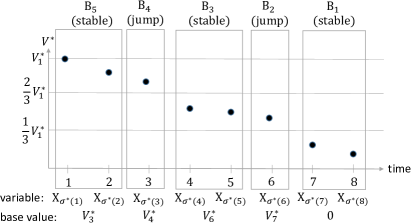
Figure 1: An illustration of our bucketing scheme.

3.3 Step 2: Guessing BaseVal

We next argue why one can assume that the BaseVal parameters are approximately known. To this end, we guess the BaseVal of each bucket from below within an additive factor of $\epsilon^{2}{\cal E}$. That is, using $\textsf{BaseGuess}(B_{j})$ to denote our guess for bucket $B_{j}$, we have

$$\textsf{BaseVal}(B_{j})~{}~{}\geq~{}~{}\textsf{BaseGuess}(B_{j})~{}~{}\geq~{}~{}\textsf{BaseVal}(B_{j})-\epsilon^{2}{\cal E}.$$ (10)

Since each bucket’s BaseGuess can be enumerated over $\{0,\epsilon^{2}{\cal E},2\epsilon^{2}{\cal E},\ldots,(1-\epsilon^{2})\cdot{\cal E}\}$, there are $1/\epsilon^{2}$ options to consider, and the total number of guesses is at most $(1/\epsilon^{2})^{2J+1}\leq(1/\epsilon^{2})^{(2/\epsilon)+1}$, which is a function of only $\epsilon$. Similarly, we guess the difference between the BaseVal of successive buckets, $B_{j}$ and $B_{j+1}$, again within an additive factor of $\epsilon^{2}{\cal E}$. That is, letting $\textsf{DeltaGuess}(B_{j})$ designate our guess for this quantity,

$$\textsf{BaseVal}(B_{j+1})-\textsf{BaseVal}(B_{j})~{}~{}\geq~{}~{}\textsf{DeltaGuess}(B_{j})~{}~{}\geq~{}~{}\textsf{BaseVal}(B_{j+1})-\textsf{BaseVal}(B_{j})-\epsilon^{2}{\cal E}.$$ (11)

As before, each bucket’s DeltaGuess can be enumerated over $\{0,\epsilon^{2}{\cal E},2\epsilon^{2}{\cal E},\ldots,(1-\epsilon^{2})\cdot{\cal E}\}$.

3.4 Step 3: The Single-Dimensional Santa Claus instance

Given $\textsf{BaseGuess}(\cdot)$ and $\textsf{DeltaGuess}(\cdot)$ for all buckets, we proceed by viewing Free-Order Prophets as an allocation problem, where we assign random variables to buckets such that each bucket receives a total load of at least $\textsf{DeltaGuess}(\cdot)$, up to a small error. Specifically, we define the following Single-Dimensional Santa Claus instance:

• Jobs and machines: There are $n$ jobs, corresponding to the random variables $X_{1},\ldots,X_{n}$. In addition, we have $2J+1$ machines, corresponding to the buckets $B_{1},\ldots,B_{2J+1}$.

• Assignment loads: When job $i\in[n]$ is assigned to machine $j\in[2J+1]$, the marginal load contribution we incur is $\ell_{ji}={\mathbb{E}}[[X_{i}-\textsf{BaseGuess}(B_{j})]^{+}]$ .

• Cardinality constraints: Jump machines can be assigned at most one job, whereas stable machines can be assigned any number of jobs.

• Load constraints: Each machine $j\in[2J+1]$ has a lower bound of $\textsf{DeltaGuess}(B_{j})$ on its total load.

Rephrasing this instance in integer programming terms, as a specialization of our generic Multi-Dimensional Santa Claus formulation, we obtain:

$$\begin{array}[]{ll}(1)\quad{\displaystyle\xi_{ji}\in\{0,1\}}&\forall\,j\in[2J+1],\,i\in[n]\\ (2)\quad{\displaystyle\sum_{j\in[2J+1]}\xi_{ji}\leq 1}&\forall\,i\in[n]\\ (3)\quad{\displaystyle\sum_{i\in[n]}\xi_{ji}\leq 1}&\forall\,j\in[2J+1]:\text{$B_{j}$ is a jump bucket}\\ (4)\quad{\displaystyle\sum_{i\in[n]}{\mathbb{E}}\left[[X_{i}-\textsf{BaseGuess}(B_{j})]^{+}\right]\cdot\xi_{ji}}{\displaystyle~{}\geq\textsf{DeltaGuess}(B_{j})}&\forall\,j\in[2J+1]:\textsf{DeltaGuess}(B_{j})>0\end{array} {}_{\textsf{Prophets}}$$ (IP)

The important observation is that our bucketing partition, formally defined in §3.2, can be massaged into forming a $2/\epsilon^{2}$-feasible solution to this program, as shown in the next lemma.

Lemma 3.2.

(IP${}_{\textsf{Prophets}}$) is $(\epsilon,0)$-sparse and admits a $2/\epsilon^{2}$-feasible solution.

Proof.

We argue that our bucketing partition of $X_{1},\ldots,X_{n}$ according to the optimal permutation $\sigma^{*}$, whose specifics were given in §3.2, can be exploited to define a $2/\epsilon^{2}$-feasible solution $\xi^{*}$ to (IP${}_{\textsf{Prophets}}$). It is worth noting that, while the latter problem is clearly $(\epsilon,0)$-feasible, the solution $\xi^{*}$ would have to satisfy $\sum_{i\in[n]}{\mathbb{E}}[[X_{i}-\textsf{BaseGuess}(B_{j})]^{+}]\cdot\xi^{*}_{ji}\leq\frac{2}{\epsilon^{2}}\cdot\textsf{DeltaGuess}(B_{j})$ for each and every bucket $B_{j}$ with $\textsf{DeltaGuess}(B_{j})>0$. For this purpose, we distinguish between two cases, depending on bucket type:

• $B_{j}$ is a jump bucket: In this case, $B_{j}$ consists of a single variable, say $X_{\sigma^{*}(t)}$, and we simply set $\xi^{*}_{j\sigma^{*}(t)}=1$ and $\xi^{*}_{ji}=0$ for every other variable.

• $B_{j}$ is a stable bucket: Here, $B_{j}$ consists of successive variables, say $X_{\sigma^{*}(t)},\ldots,X_{\sigma^{*}(t+k)}$. Letting $\overline{k}$ be the maximal index for which $\sum_{\kappa=0}^{\overline{k}}{\mathbb{E}}\left[[X_{\sigma^{*}(t+\kappa)}-\textsf{BaseGuess}(B_{j})]^{+}\right]\leq 2{\cal E}$, we set $\xi^{*}_{j\sigma^{*}(t)}=\cdots=\xi^{*}_{j\sigma^{*}(t+\overline{k})}=1$ and $\xi^{*}_{ji}=0$ for every other variable.

We first notice that constraints (1)-(3) are satisfied since $\xi^{*}$ is a binary vector, assigning each random variable to at most one machine, and exactly one variable to each jump machine. Therefore, to conclude the $2/\epsilon^{2}$-feasibility of $\xi^{*}$, it remains to show that for every bucket $B_{j}$ with $\textsf{DeltaGuess}(B_{j})>0$,

$$\frac{\sum_{i\in[n]}{\mathbb{E}}\left[[X_{i}-\textsf{BaseGuess}(B_{j})]^{+}\right]\cdot\xi^{*}_{ji}}{\textsf{DeltaGuess}(B_{j})}\in\left[1,\frac{2}{\epsilon^{2}}\right]\ .$$

Again, we diverge by bucket type:

• $B_{j}$ is a jump bucket: In this case, the required lower bound is derived by noting that

  $${\textstyle\sum_{i\in[n]}}{\mathbb{E}}\left[[X_{i}-\textsf{BaseGuess}(B_{j})]^{+}\right]\cdot\xi^{*}_{ji} = {\mathbb{E}}\left[[X_{\sigma^{*}(t)}-\textsf{BaseGuess}(B_{j})]^{+}\right]$$

  $$\geq {\mathbb{E}}\left[[X_{\sigma^{*}(t)}-\textsf{BaseVal}(B_{j})]^{+}\right]$$

  $$= \textsf{BaseVal}(B_{j+1})-\textsf{BaseVal}(B_{j})~{}\geq~{}\textsf{DeltaGuess}(B_{j})\ ,$$

  where the inequalities follow from (10) and (11), respectively. To upper bound, observe that

  $${\mathbb{E}}\left[[X_{\sigma^{*}(t)}-\textsf{BaseGuess}(B_{j})]^{+}\right] ~{}\leq~{}{\mathbb{E}}\left[[X_{\sigma^{*}(t)}]^{+}\right]$$

  $$~{}\leq~{}\textsc{OPT}~{}~{}\leq~{}~{}(1+\epsilon)\cdot{\cal E}~{}~{}\leq~{}~{}\frac{2}{\epsilon^{2}}\cdot\textsf{DeltaGuess}(B_{j})\ .$$

  Here, the second inequality is attained by noting that any permutation ending with $X_{\sigma^{*}(t)}$ has an expected reward of at least ${\mathbb{E}}[[X_{\sigma^{*}(t)}]^{+}]$, meaning that OPT is at least this large. The fourth inequality holds since $\textsf{DeltaGuess}(B_{j})\geq\epsilon^{2}{\cal E}$, due to restricting the possible values for this guess to $\{0,\epsilon^{2}{\cal E},2\epsilon^{2}{\cal E},\ldots,(1-\epsilon^{2})\cdot{\cal E}\}$ (see §3.3), and since we are considering buckets with $\textsf{DeltaGuess}(B_{j})>0$, where constraint (4) is active.

• $B_{j}$ is a stable bucket: In this case, the upper bound immediately follows by noting that

  $$\textstyle\sum_{i\in[n]}{\mathbb{E}}\left[[X_{i}-\textsf{BaseGuess}(B_{j})]^{+}\right]\cdot\xi^{*}_{ji} = \textstyle\sum_{\kappa=0}^{\overline{k}}{\mathbb{E}}\left[[X_{\sigma^{*}(t+\kappa)}-\textsf{BaseGuess}(B_{j})]^{+}\right]$$

  $$\leq 2{\cal E}~{}~{}\leq~{}~{}\frac{2}{\epsilon^{2}}\cdot\textsf{DeltaGuess}(B_{j})\ ,$$

  where the first inequality holds by definition of $\overline{k}$. As far as the lower bound is concerned, note that when $\sum_{\kappa=0}^{\overline{k}}{\mathbb{E}}[[X_{\sigma^{*}(t+\kappa)}-\textsf{BaseGuess}(B_{j})]^{+}]\geq{\cal E}$, we are clearly done, since $\textsf{DeltaGuess}(B_{j})\leq{\cal E}$, as explained in the first item. In the opposite case, it follows that $\overline{k}=k$, implying in turn that

  $$\textstyle\sum_{i\in[n]}{\mathbb{E}}\left[[X_{i}-\textsf{BaseGuess}(B_{j})]^{+}\right]\cdot\xi^{*}_{ji} = \textstyle\sum_{\kappa=0}^{k}{\mathbb{E}}\left[[X_{\sigma^{*}(t+\kappa)}-\textsf{BaseGuess}(B_{j})]^{+}\right]$$

  $$\geq \textstyle\sum_{\kappa=0}^{k}{\mathbb{E}}\left[[X_{\sigma^{*}(t+\kappa)}-V^{*}_{t+\kappa+1}]^{+}\right]$$

  $$= \textsf{BaseVal}(B_{j+1})-\textsf{BaseVal}(B_{j})$$

  $$\geq \textsf{DeltaGuess}(B_{j})\ ,$$

  where the first inequality holds since $V_{t}^{*}\geq\cdots\geq V_{t+\kappa+1}^{*}=\textsf{BaseVal}(B_{j})\geq\textsf{BaseGuess}(B_{j})$. ∎

Consequently, by recalling that the number of machines involved is $2J+1=O(1/\epsilon)$, Theorem 2.2 implies that we can compute in EPTAS time a cardinality-feasible assignment where the load of each machine $j$ is at least $(1-\epsilon)\cdot\textsf{DeltaGuess}(B_{j})$. This can be formally summarized as follows.

Corollary 3.3.

There is an EPTAS for computing a cardinality-feasible variable-to-machine assignment $\mathbf{x}\in\{0,1\}^{(2J+1)\times n}$ such that every machine $j\in[2J+1]$ receives a total load of $\sum_{i\in[n]}\ell_{ji}x_{ji}\geq(1-\epsilon)\cdot\textsf{DeltaGuess}(B_{j})$.

3.5 Final permutation and its value guarantee

Given the assignment vector $\mathbf{x}$ due to Corollary 3.3, we construct a probing permutation as follows. The last variables to be inspected are those assigned to the first machine (i.e., the one corresponding to $B_{1}$); their internal order is arbitrary. Just before them, we will inspect those assigned to the second machine (corresponding to $B_{2})$, again in an arbitrary order, and so on. Letting $\sigma$ be the resulting permutation, we show in the remainder of this section that $V(\sigma)\geq(1-7\epsilon)\cdot\textsc{OPT}$, thereby establishing Theorem 3.1.

We begin by defining the sequence of values $R_{1},\ldots,R_{n}$ attained for suffixes of the permutation $\sigma$. Letting $R_{n+1}=0$, we recursively set $R_{t}=\mathbb{E}[\max\{X_{\sigma(t)},R_{t+1}\}]$ for $1\leq t\leq n$, noting that $R_{1}=V(\sigma)$. We say that our permutation $\sigma$ is behind schedule at time $t\in[n]$ if $R_{t+1}<\textsf{BaseGuess}(B^{-1}_{X_{\sigma(t)}})$, where $B^{-1}_{X_{\sigma(t)}}$ is the bucket to which $X_{\sigma(t)}$ is assigned; otherwise, $\sigma$ is ahead of schedule at that time. Let $t_{\min}$ be the minimal time when we are ahead of schedule, i.e., satisfy $R_{t_{\min}+1}\geq\textsf{BaseGuess}(B^{-1}_{X_{\sigma(t_{\min})}})$. This index is well-defined, since we are always ahead of schedule at time $n$, as $R_{n+1}=0=\textsf{BaseVal}(B_{1})=\textsf{BaseGuess}(B_{1})$, where the last equality follows from (10) and the non-negativity of BaseGuess.

Now, noting that the value of our algorithm in terms of the permutation $\sigma$ is

$$\textstyle V(\sigma)~{}=~{}R_{t_{\min}}+\sum_{t<t_{\min}}(R_{t}-R_{t+1})\ ,$$ (12)

we proceed by lower bounding each of these terms.

Claim 3.4.

The first term in (12) can be lower bounded as

$$R_{t_{\min}}~{}~{}\geq~{}~{}\textsf{BaseVal}\left(B^{-1}_{X_{\sigma(t_{\min})}}\right)+(1-\epsilon)\cdot\textsf{DeltaGuess}\left(B^{-1}_{X_{\sigma(t_{\min})}}\right)-2\epsilon\cdot\textsc{OPT}\ .$$

Proof.

First, we know that $R_{t_{\min}}$ equals

$${\mathbb{E}}\left[\max\{X_{\sigma(t_{\min})},R_{t_{\min}+1}\}\right] \geq {\mathbb{E}}\left[\max\left\{X_{\sigma(t_{\min})},\textsf{BaseGuess}\left(B^{-1}_{X_{\sigma(t_{\min})}}\right)\right\}\right]$$

$$= \textsf{BaseGuess}\left(B^{-1}_{X_{\sigma(t_{\min})}}\right)+{\mathbb{E}}\left[\left[X_{\sigma(t_{\min})}-\textsf{BaseGuess}\left(B^{-1}_{X_{\sigma(t_{\min})}}\right)\right]^{+}\right].$$

The crucial observation is that the term ${\mathbb{E}}[[X_{\sigma(t_{\min})}-\textsf{BaseGuess}(B^{-1}_{X_{\sigma(t_{\min})}})]^{+}]$ represents the load contribution due to assigning job $\sigma(t_{\min})$ to the machine corresponding to bucket $B^{-1}_{X_{\sigma(t_{\min})}}$. When the latter is a jump bucket, our cardinality constraints ensure that job $\sigma(t_{\min})$ is the only one assigned, implying that ${\mathbb{E}}[[X_{\sigma(t_{\min})}-\textsf{BaseGuess}(B^{-1}_{X_{\sigma(t_{\min})}})]^{+}]\geq(1-\epsilon)\cdot\textsf{DeltaGuess}(B^{-1}_{X_{\sigma(t_{\min})}})$ by Corollary 3.3. In the other scenario of a stable bucket, we actually have $\textsf{DeltaGuess}(B^{-1}_{X_{\sigma(t_{\min})}})\leq\epsilon\cdot\textsc{OPT}$, since this bucket does not cross over an integer multiple of $\epsilon\cdot\textsc{OPT}$, by definition (see §3.2). In either case, we have just shown that

$$R_{t_{\min}} \geq \textsf{BaseGuess}\left(B^{-1}_{X_{\sigma(t_{\min})}}\right)+(1-\epsilon)\cdot\textsf{DeltaGuess}\left(B^{-1}_{X_{\sigma(t_{\min})}}\right)-\epsilon\cdot\textsc{OPT}$$ (13)

$$\geq \textsf{BaseVal}\left(B^{-1}_{X_{\sigma(t_{\min})}}\right)+(1-\epsilon)\cdot\textsf{DeltaGuess}\left(B^{-1}_{X_{\sigma(t_{\min})}}\right)-2\epsilon\cdot\textsc{OPT}\ ,$$

where the second inequality uses (10) and that ${\cal E}\leq\textsc{OPT}$. ∎

Next, we lower bound the second term.

Claim 3.5.

The second term in (12) can be lower bounded as

$$\textstyle\sum_{t<t_{\min}}(R_{t}-R_{t+1})~{}~{}\geq~{}~{}(1-\epsilon)\cdot\sum_{j>B^{-1}_{X_{\sigma(t_{\min})}}}\Big{(}\textsf{BaseVal}(B_{j+1})-\textsf{BaseVal}(B_{j})\Big{)}-3\epsilon\cdot\textsc{OPT}.$$

Proof.

We first simplify the LHS of the claim,

$$\sum_{t<t_{min}}(R_{t}-R_{t+1})~{}~{}=~{}~{}\sum_{t<t_{min}}\left({\mathbb{E}}\left[\max\{X_{\sigma(t)},R_{t+1}\}\right]-R_{t+1}\right)~{}~{}=~{}~{}\sum_{t<t_{min}}{\mathbb{E}}\left[[X_{\sigma(t)}-R_{t+1}]^{+}\right]\ .$$

The expected gain at any time $t<t_{\min}$ satisfies $\mathbb{E}[[X_{\sigma(t)}-R_{t+1}]^{+}]\geq\mathbb{E}[[X_{\sigma(t)}-\textsf{BaseGuess}(B^{-1}_{X_{\sigma(t)}})]^{+}]$. Summing this bound over all variables assigned to machine $j\in[2J+1]$, we have

$$\sum_{t:B^{-1}_{X_{\sigma(t)}}=j}\mathbb{E}[[X_{\sigma(t)}-R_{t+1}]^{+}] \geq \sum_{t:B^{-1}_{X_{\sigma(t)}}=j}\mathbb{E}[[X_{\sigma(t)}-\textsf{BaseGuess}(B_{j})]^{+}]$$

$$= \sum_{i\in[n]}\ell_{ji}x_{ji}\qquad\geq\qquad(1-\epsilon)\cdot\textsf{DeltaGuess}(B_{j}),$$

where the last inequality follows from Corollary 3.3. Thus, we get

$$\sum_{t<t_{\min}}(R_{t}-R_{t+1})~{}~{}=~{}~{}\sum_{t<t_{\min}}{\mathbb{E}}\left[[X_{\sigma(t)}-R_{t+1}]^{+}\right] \geq \sum_{j>B^{-1}_{X_{\sigma(t_{\min})}}}\sum_{t:B^{-1}_{X_{\sigma(t)}}=j}{\mathbb{E}}\left[[X_{\sigma(t)}-R_{t+1}]^{+}\right]$$

$$\geq (1-\epsilon)\cdot\sum_{j>B^{-1}_{X_{\sigma(t_{\min})}}}\textsf{DeltaGuess}(B_{j})\ .$$

Now, given the lower bound on $\textsf{DeltaGuess}(B_{j})$ in (11), it follows that

$$\sum_{t<t_{\min}}(R_{t}-R_{t+1}) \geq (1-\epsilon)\cdot\sum_{j>B^{-1}_{X_{\sigma(t_{\min})}}}\Big{(}\textsf{BaseVal}(B_{j+1})-\textsf{BaseVal}(B_{j})\Big{)}-\epsilon^{2}{\cal E}\cdot(2J+1)$$

$$\geq (1-\epsilon)\cdot\sum_{j>B^{-1}_{X_{\sigma(t_{\min})}}}\Big{(}\textsf{BaseVal}(B_{j+1})-\textsf{BaseVal}(B_{j})\Big{)}-3\epsilon\cdot\textsc{OPT},$$

where the last inequality follows by recalling that $J\leq 1/\epsilon$ and that ${\cal E}\leq\textsc{OPT}$. ∎

Combining the two claims with (12), our permutation $\sigma$ attains a value of

$$V(\sigma) \geq \Big{(}\textsf{BaseVal}\left(B^{-1}_{X_{\sigma(t_{\min})}}\right)+(1-\epsilon)\cdot\textsf{DeltaGuess}\left(B^{-1}_{X_{\sigma(t_{\min})}}\right)-2\epsilon\cdot\textsc{OPT}\Big{)}$$

$$\mbox{}+\textstyle(1-\epsilon)\cdot\sum_{j>B^{-1}_{X_{\sigma(t_{\min})}}}\Big{(}\textsf{BaseVal}(B_{j+1})-\textsf{BaseVal}(B_{j})\Big{)}-3\epsilon\cdot\textsc{OPT}$$

$$\geq (1-7\epsilon)\cdot\textsc{OPT}\ .$$

4 Non-Adaptive ProbeMax

In what follows, we utilize our approximation scheme for Multi-Dimensional Santa Claus to design an EPTAS for the non-adaptive ProbeMax problem, whose precise performance guarantees are stated in Theorem 1.2. Interestingly, our reduction for this application will create a single-machine Santa Claus instance, albeit resorting to multi-dimensional load vectors.

4.1 Preliminaries

We remind the reader that an instance of the non-adaptive ProbeMax problem consists of $n$ independent non-negative random variables $X_{1},\ldots,X_{n}$. For any subset $S\subseteq[n]$, we make use of ${\cal M}(S):=\max_{i\in S}X_{i}$ to designate the maximum value over the sub-collection of variables $\{X_{i}\}_{i\in S}$. Given an additional parameter $k$, our objective is to identify a subset $S\subseteq[n]$ of cardinality at most $k$ that maximizes ${\mathbb{E}}[{\cal M}(S)]$.

By referring to the technical discussion of Chen et al. [CHL⁺16, App. C] in this context, the following assumptions can be made without loss of generality:

1. The inverse accuracy level $1/\epsilon$ is an integer.

2. Letting $S^{*}$ be an optimal subset, an estimate ${\cal E}\in\big{[}(1-\frac{1}{e})\cdot{\mathbb{E}}[{\cal M}(S^{*})]~{},~{}{\mathbb{E}}[{\cal M}(S^{*})]\big{]}$ for the optimal expected maximum is known in advance.

3. The variables $X_{1},\ldots,X_{n}$ are defined over the same support, ${\cal V}=\big{\{}0,\epsilon{\cal E},2\epsilon{\cal E},\ldots,\frac{\cal E}{\epsilon}\big{\}}$.

In addition, we assume without loss of generality that ${\mathbb{P}}(X_{i}=0)\geq\epsilon$ for every $i\in[n]$. This property can be enforced by defining $\tilde{X}_{i}=I_{i}X_{i}$, where $I_{i}$ is an indicator variable taking a zero value with probability $\epsilon$. Letting $\tilde{\cal M}(S):=\max_{i\in S}\tilde{X}_{i}$, it is easy to verify that ${\mathbb{E}}[\tilde{\cal M}(S)]\geq(1-\epsilon)\cdot{\mathbb{E}}[{\cal M}(S)]$ for any subset $S\subseteq[n]$, and that $\tilde{\cal M}(S)$ is stochastically smaller than ${\cal M}(S)$, meaning that the expected maximum can only increase when we restore the original variables.

4.2 Step 1: Guessing the CDF of the optimal maximum value

We begin by approximately guessing the cumulative distribution function of the unknown random variable ${\cal M}(S^{*})$. Specifically, noting that ${\mathbb{P}}({\cal M}(S^{*})\leq v)$ is monotone non-decreasing in $v$, let $v_{\mathrm{light}}\in{\cal V}$ be the maximal value $v$ for which ${\mathbb{P}}({\cal M}(S^{*})\leq v)<2\epsilon^{2}$; when no such value exists, $v_{\mathrm{light}}=-\infty$. Similarly, let $v_{\mathrm{heavy}}\in{\cal V}$ be the maximal value for which ${\mathbb{P}}({\cal M}(S^{*})\leq v)<1-\epsilon^{2}$, where $v_{\mathrm{heavy}}=\infty$ when no such value exists. Having guessed both $v_{\mathrm{light}}$ and $v_{\mathrm{heavy}}$, we define the interval ${\cal V}_{\mathrm{critical}}={\cal V}\cap[v_{\mathrm{light}},v_{\mathrm{heavy}}]$ and proceed as follows:

• For every value $v\in{\cal V}_{\mathrm{critical}}\setminus\{v_{\mathrm{light}}\}$, we guess an additive over-estimate $\tilde{p}_{\leq v}$ for the probability ${\mathbb{P}}({\cal M}(S^{*})\leq v)$ that satisfies

  $${\mathbb{P}}\left({\cal M}(S^{*})\leq v\right)\quad\leq\quad\tilde{p}_{\leq v}\quad<\quad{\mathbb{P}}\left({\cal M}(S^{*})\leq v\right)+\epsilon^{2}\ .$$ (14)

  As such, each $\tilde{p}_{\leq v}$ value is restricted to the set $\{2\epsilon^{2},3\epsilon^{2},\ldots,1-\epsilon^{2}\}$, implying that the total number of guesses required to derive these estimates is only $O((\frac{1}{\epsilon^{2}})^{O(|{\cal V}|)})=O((\frac{1}{\epsilon})^{O(1/\epsilon^{2})})$.

• In addition, we guess a single multiplicative over-estimate $\tilde{p}_{\leq v_{\mathrm{light}}}$ for the probability ${\mathbb{P}}({\cal M}(S^{*})\leq v_{\mathrm{light}})$ that satisfies

  $${\mathbb{P}}\left({\cal M}(S^{*})\leq v_{\mathrm{light}}\right)\quad\leq\quad\tilde{p}_{\leq v_{\mathrm{light}}}\quad\leq\quad 2\cdot{\mathbb{P}}\left({\cal M}(S^{*})\leq v_{\mathrm{light}}\right)\ .$$ (15)

  For this purpose, we observe that ${\mathbb{P}}({\cal M}(S^{*})\leq v_{\mathrm{light}})\geq\prod_{i\in S^{*}}{\mathbb{P}}(X_{i}=0)\geq\epsilon^{k}$, by our initial assumption, and we can restrict our estimate to powers of $2$ within the interval $[\epsilon^{k},2\epsilon^{2}]$. Therefore, the number of required guesses is $O(k\log\frac{1}{\epsilon})$.

4.3 Why nearly matching the distribution suffices

Moving forward, our objective would be to identify a feasible subset $\tilde{S}\subseteq[n]$ for which the cumulative distribution function of ${\cal M}(\tilde{S})$ nearly matches that of ${\cal M}(S^{*})$. To formalize this notion, we say that $\tilde{S}$ is a CDF-equivalent subset when ${\mathbb{P}}({\cal M}(\tilde{S})\leq v)\leq(1+\epsilon^{2})\cdot\tilde{p}_{\leq v}+\epsilon^{2}$ for every $v\in{\cal V}_{\mathrm{critical}}$. We first establish the performance guarantee of such subsets.

Lemma 4.1.

Let $\tilde{S}\subseteq[n]$ be CDF-equivalent subset. Then, ${\mathbb{E}}[{\cal M}(\tilde{S})]\geq(1-21\epsilon)\cdot{\mathbb{E}}[{\cal M}(S^{*})]$.

Proof.

We begin by arguing that ${\mathbb{P}}({\cal M}(\tilde{S})\leq v)\leq(1+\epsilon^{2})\cdot{\mathbb{P}}({\cal M}(S^{*})\leq v)+9\epsilon^{2}$ for every $v\in{\cal V}$:

• When $v\leq v_{\mathrm{light}}$, we have ${\mathbb{P}}({\cal M}(\tilde{S})\leq v)\leq{\mathbb{P}}({\cal M}(\tilde{S})\leq v_{\mathrm{light}})\leq(1+\epsilon^{2})\cdot\tilde{p}_{\leq v_{\mathrm{light}}}+\epsilon^{2}$ since $\tilde{S}$ is a CDF-equivalent subset. Now by combining with the right inequality in (15), we get

  $${\mathbb{P}}\left({\cal M}(\tilde{S})\leq v\right)~{}~{}\leq~{}~{}2(1+\epsilon^{2})\cdot{\mathbb{P}}\left({\cal M}(S^{*})\leq v_{\mathrm{light}}\right)+\epsilon^{2}~{}~{}\leq~{}~{}9\epsilon^{2},$$

  where the last inequality holds since ${\mathbb{P}}({\cal M}(S^{*})\leq v_{\mathrm{light}})<2\epsilon^{2}$ by definition of $v_{\mathrm{light}}$.

• When $v_{\mathrm{light}}<v\leq v_{\mathrm{heavy}}$, we have ${\mathbb{P}}({\cal M}(\tilde{S})\leq v)\leq(1+\epsilon^{2})\cdot\tilde{p}_{\leq v}+\epsilon^{2}$ since $\tilde{S}$ is a CDF-equivalent subset. Combining with the right inequality in (14), we get

  $${\mathbb{P}}\left({\cal M}(\tilde{S})\leq v\right) \leq (1+\epsilon^{2})\cdot\left({\mathbb{P}}\left({\cal M}(S^{*})\leq v\right)+\epsilon^{2}\right)+\epsilon^{2}~{}\leq~{}~{}(1+\epsilon^{2})\cdot{\mathbb{P}}\left({\cal M}(S^{*})\leq v\right)+3\epsilon^{2}\ .$$

• When $v>v_{\mathrm{heavy}}$, we have ${\mathbb{P}}({\cal M}(\tilde{S})\leq v)\leq 1\leq{\mathbb{P}}({\cal M}(S^{*})\leq v)+\epsilon^{2}\ ,$ where the second inequality holds since ${\mathbb{P}}({\cal M}(S^{*})\leq v)\geq 1-\epsilon^{2}$ for every $v>v_{\mathrm{heavy}}$, by definition of $v_{\mathrm{heavy}}$.

Noting that ${\cal M}(\tilde{S})$ and ${\cal M}(S^{*})$ are both defined over the support ${\cal V}=\{0,\epsilon{\cal E},2\epsilon{\cal E},\ldots,\frac{\cal E}{\epsilon}\}$, we can now relate between the expectations of ${\cal M}(\tilde{S})$ and ${\cal M}(S^{*})$ through the tail sum formula as follows:

$${\mathbb{E}}\left[{\cal M}(\tilde{S})\right] = \epsilon{\cal E}\cdot\sum_{v\in{\cal V}}\left(1-{\mathbb{P}}\left({\cal M}(\tilde{S})\leq v\right)\right)$$

$$\geq \epsilon{\cal E}\cdot\sum_{v\in{\cal V}}\left(1-\left((1+\epsilon^{2})\cdot{\mathbb{P}}\left({\cal M}(S^{*})\leq v\right)+9\epsilon^{2}\right)\right)$$

$$\geq (1-\epsilon^{2})\cdot\epsilon{\cal E}\cdot\sum_{v\in{\cal V}}\left(1-{\mathbb{P}}\left({\cal M}(S^{*})\leq v\right)\right)-10\epsilon^{3}{\cal E}\cdot|{\cal V}|$$

$$\geq \left(1-\epsilon^{2}\right)\cdot{\mathbb{E}}\left[{\cal M}(S^{*})\right]-20\epsilon{\cal E}~{}~{}\geq~{}~{}(1-21\epsilon)\cdot{\mathbb{E}}\left[{\cal M}(S^{*})\right]\ ,$$

where the last two inequalities use $|{\cal V}|=\frac{1}{\epsilon^{2}}+1\leq\frac{2}{\epsilon^{2}}$ for $\epsilon\in(0,1)$ and ${\cal E}\leq{\mathbb{E}}[{\cal M}(S^{*})]$. ∎

4.4 Step 2: The Multi-Dimensional Santa Claus instance

We proceed to formulate an integer program that expresses CDF-related inequalities as linear covering constraints. To this end, for every $i\in[n]$ and $v\in{\cal V}_{\mathrm{critical}}$, let us introduce the non-negative constant $\ell_{iv}=\ln(\frac{1}{{\mathbb{P}}(X_{i}\leq v)})$, noting that the latter denominator is strictly positive, by our initial assumption that ${\mathbb{P}}(X_{i}=0)\geq\epsilon$. Now consider the following feasibility-type integer problem:

$$\begin{array}[]{ll}(1)\quad{\displaystyle\xi_{i}\in\{0,1\}}&\forall\,i\in[n]\\ (2)\quad{\displaystyle\sum_{i\in[n]}\xi_{i}\leq k}\\ (3)\quad{\displaystyle\sum_{i\in[n]}\ell_{iv}\xi_{i}\geq\ln\left(\frac{1}{\tilde{p}_{\leq v}}\right)}&\forall\,v\in{\cal V}_{\mathrm{critical}}\end{array}$$ (IP_CDF)

Interpretation.

A close inspection of (IP_CDF) reveals that we have just written an integer programming formulation of the Multi-Dimensional Santa Claus problem on a single machine:

• Jobs and machines: There are $n$ jobs, corresponding to the random variables $X_{1},\ldots,X_{n}$. These jobs can potentially be assigned to a single machine, which captures the subset of variables to be probed. From this perspective, the binary variable $\xi_{i}$ indicates whether the random variable $X_{i}$ is picked as part of the subset we construct.

• Assignment loads: When job $i\in[n]$ is chosen, the marginal load contribution we incur is specified by the $|{\cal V}_{\mathrm{critical}}|$-dimensional vector $\ell_{i}=(\ell_{iv})$.

• Cardinality constraints: At most $k$ jobs can be assigned.

• Load constraints: Along any dimension $v\in{\cal V}_{\mathrm{critical}}$, its total load is lower bounded by $\ln(\frac{1}{\tilde{p}_{\leq v}})$.

Feasibility of (IP_CDF).

The next lemma argues that the resulting Multi-Dimensional Santa Claus instance meets the technical condition underlying Theorem 2.2, in the sense of admitting a $\rho$-feasible solution, for some constant $\rho\geq 1$ depending only on $\epsilon$.

Lemma 4.2.

(IP_CDF) is $(\epsilon,0)$-sparse and admits a $1/\epsilon^{4}$-feasible solution.

Proof.

To establish the desired claim, we show that the optimal subset $S^{*}$ for our original ProbeMax problem induces a $1/\epsilon^{4}$-feasible solution $\xi^{*}$ to (IP_CDF). This solution is simply the incidence vector of $S^{*}$, meaning that $\xi^{*}_{i}=1$ if and only if $i\in S^{*}$.

First, constraints (1) and (2) are clearly satisfied, since $\xi^{*}$ is a binary vector, in which the number of assigned jobs is given by $\sum_{i\in[n]}\xi_{i}^{*}=|S^{*}|\leq k$. To verify constraint (3), since we have previously stated that  (IP_CDF) is $(\epsilon,0)$-feasible, the solution $\xi^{*}$ has to satisfy $\sum_{i\in[n]}\ell_{iv}\xi_{i}^{*}\leq\frac{1}{\epsilon^{4}}\cdot\ln(\frac{1}{\tilde{p}_{\leq v}})$ for every $v\in{\cal V}_{\mathrm{critical}}$. To this end, note that

$$\sum_{i\in[n]}\ell_{iv}\xi_{i}^{*}~{}~{}=~{}~{}\sum_{i\in S^{*}}\ln\left(\frac{1}{{\mathbb{P}}(X_{i}\leq v)}\right) = \ln\left(\frac{1}{\prod_{i\in S^{*}}{\mathbb{P}}(X_{i}\leq v)}\right)$$

$$= \ln\left(\frac{1}{{\mathbb{P}}(\max_{i\in S^{*}}X_{i}\leq v)}\right)~{}~{}=~{}~{}\ln\left(\frac{1}{{\mathbb{P}}({\cal M}(S^{*})\leq v)}\right)\ ,$$

where the third equality holds since $X_{1},\ldots,X_{n}$ are independent. As a result, we conclude that $\xi^{*}$ is a $1/\epsilon^{4}$-feasible solution, by considering two cases:

• For $v\in{\cal V}_{\mathrm{critical}}\setminus\{v_{\mathrm{light}}\}$, we have $\sum_{i\in[n]}\ell_{iv}\xi_{i}^{*}\in[\ln(\frac{1}{\tilde{p}_{\leq v}}),\ln(\frac{1}{\tilde{p}_{\leq v}-\epsilon^{2}})]$, as an immediate consequence of the inequalities in (14). In this case, we observe that $\ln(\frac{1}{\tilde{p}_{\leq v}-\epsilon^{2}})\leq\frac{1}{\epsilon^{4}}\cdot\ln(\frac{1}{\tilde{p}_{\leq v}})$. Indeed, since $\tilde{p}_{\leq v}$ is restricted to the set $\{2\epsilon^{2},3\epsilon^{2},\ldots,1-\epsilon^{2}\}$, we necessarily have $\tilde{p}_{\leq v}\leq 1-\epsilon^{2}$ and therefore $\ln(\frac{1}{\tilde{p}_{\leq v}})\geq-\ln(1-\epsilon^{2})\geq\epsilon^{2}$. On the other hand, since $v>v_{\mathrm{light}}$, it follows that $\tilde{p}_{\leq v}\geq 2\epsilon^{2}$ and $\ln(\frac{1}{\tilde{p}_{\leq v}-\epsilon^{2}})\leq\ln(\frac{1}{\epsilon^{2}})\leq\frac{1}{\epsilon^{2}}$.

• For $v_{\mathrm{light}}$, we have $\sum_{i\in[n]}\ell_{iv_{\mathrm{light}}}\xi_{i}^{*}\in[\ln(\frac{1}{\tilde{p}_{\leq v_{\mathrm{light}}}}),\ln(\frac{2}{\tilde{p}_{\leq v_{\mathrm{light}}}})]$ as a consequence of the inequalities in (15). Here, we claim that $\ln(\frac{2}{\tilde{p}_{\leq v_{\mathrm{light}}}})\leq 2\cdot\ln(\frac{1}{\tilde{p}_{\leq v_{\mathrm{light}}}})$. To this end, by recalling that $\tilde{p}_{\leq v_{\mathrm{light}}}\leq 2\epsilon^{2}\leq\frac{1}{2}$ for $\epsilon\in(0,\frac{1}{2})$, we have $\frac{2}{\tilde{p}_{\leq v_{\mathrm{light}}}}\leq(\frac{1}{\tilde{p}_{\leq v_{\mathrm{light}}}})^{2}$, and the desired inequality is obtained by taking $\ln$ on both sides. ∎

4.5 Final subset and its value guarantee

As an immediate byproduct of Lemma 4.2, due to considering a single-machine $O(1/\epsilon^{2})$-Dimensional Santa Claus instance, Theorem 2.2 allows us to compute in EPTAS time a cardinality-feasible subset of variables, where the load constraint along any dimension is violated by a factor of at most $\delta$, for any fixed $\delta>0$. This claim can be formally stated as follows.

Corollary 4.3.

There is an EPTAS for computing a vector $\xi\in\{0,1\}^{n}$ satisfying $\sum_{i\in[n]}\xi_{i}\leq k$ as well as $\sum_{i\in[n]}\ell_{iv}\xi_{i}\geq(1-\delta)\cdot\ln(\frac{1}{\tilde{p}_{\leq v}})$, for every $v\in{\cal V}_{\mathrm{critical}}$.

Now let $\tilde{S}\subseteq[n]$ be the subset of random variable indices corresponding to the choices made by $\xi$, meaning that $\tilde{S}=\{i\in[n]:\xi_{i}=1\}$. This subset clearly picks at most $k$ variables, for any choice of $\delta$. We conclude our analysis by proving that ${\mathbb{E}}[{\cal M}(\tilde{S})]\geq(1-21\epsilon)\cdot{\mathbb{E}}[{\cal M}(S^{*})]$ when Corollary 4.3 is instantiated with $\delta=\frac{\epsilon^{3}}{6}$.

Proof of Theorem 1.2.

Based on Lemma 4.1, to prove the desired relation between ${\mathbb{E}}[{\cal M}(\tilde{S})]$ and ${\mathbb{E}}[{\cal M}(S^{*})]$, it suffices to show that $\tilde{S}$ is a CDF-equivalent subset, meaning that ${\mathbb{P}}({\cal M}(\tilde{S})\leq v)\leq(1+\epsilon^{2})\cdot\tilde{p}_{\leq v}+\epsilon^{2}$ for every $v\in{\cal V}_{\mathrm{critical}}$. For this purpose, note that

$${\mathbb{P}}\left({\cal M}(\tilde{S})\leq v\right) = \textstyle{\mathbb{P}}\left(\max_{i\in\tilde{S}}X_{i}\leq v\right)~{}~{}=~{}~{}\prod_{i\in\tilde{S}}{\mathbb{P}}\left(X_{i}\leq v\right)$$

$$= \textstyle\exp\Big{\{}-\sum_{i\in\tilde{S}}\ln\Big{(}\frac{1}{{\mathbb{P}}\left(X_{i}\leq v\right)}\Big{)}\Big{\}}~{}~{}=~{}~{}\exp\Big{\{}-\sum_{i\in[n]}\ell_{iv}\xi_{i}\Big{\}}$$

$$\leq \textstyle\exp\Big{\{}-\Big{(}1-\frac{\epsilon^{3}}{6}\Big{)}\cdot\ln\Big{(}\frac{1}{\tilde{p}_{\leq v}}\Big{)}\Big{\}}~{}~{}=~{}~{}\tilde{p}_{\leq v}^{1-\epsilon^{3}/6}\ ,$$

where the second equality follows from the independence of $X_{1},\ldots,X_{n}$, and the inequality above holds since $\sum_{i\in[n]}\ell_{iv}\xi_{i}\geq(1-\frac{\epsilon^{3}}{6})\cdot\ln(\frac{1}{\tilde{p}_{\leq v}})$, via the instantiation of Corollary 4.3 with $\delta=\frac{\epsilon^{3}}{6}$.

Now, to obtain an upper bound on $\tilde{p}_{\leq v}^{1-\epsilon^{3}/6}$, note that the differentiable function $x\mapsto x^{1-\epsilon^{3}/6}$ is concave over $[0,\infty)$. Therefore, by applying the gradient inequality, $\tilde{p}_{\leq v}^{1-\epsilon^{3}/6}\leq x^{1-\epsilon^{3}/6}+(1-\frac{\epsilon^{3}}{6})\cdot x^{-\epsilon^{3}/6}\cdot(p-x)$ for every $x\geq 0$. Plugging in $x=\epsilon^{3}$, we get

$$\tilde{p}_{\leq v}^{1-\epsilon^{3}/6}~{}~{}\leq~{}~{}\underbrace{\epsilon^{3(1-\epsilon^{3}/6)}}_{\leq\epsilon^{2}}+\left(1-\frac{\epsilon^{3}}{6}\right)\cdot\epsilon^{-\epsilon^{3}/2}\cdot\left(\tilde{p}_{\leq v}-\epsilon^{3}\right)~{}\leq~{}\epsilon^{2}+\epsilon^{-\epsilon^{3}/2}\cdot\tilde{p}_{\leq v}~{}~{}\leq~{}~{}(1+\epsilon^{2})\cdot\tilde{p}_{\leq v}+\epsilon^{2}\ ,$$

where the last inequality holds since $\epsilon^{-\epsilon^{3}/2}~{}=~{}e^{(\epsilon^{3}/2)\cdot\ln(1/\epsilon)}~{}\leq~{}e^{\epsilon^{2}/2}~{}\leq~{}1+\epsilon^{2}$. ∎

5 Adaptive ProbeMax

In what follows, we employ our algorithmic framework to design an EPTAS for the adaptive ProbeMax problem, as formally stated in Theorem 1.3. This application would require the full-blown features of our Multi-Dimensional Santa Claus problem, as provided in §2.

5.1 Preliminaries

Similarly to its non-adaptive variant, an instance of the adaptive ProbeMax problem consists of $n$ independent non-negative random variables $X_{1},\ldots,X_{n}$. For any subset $S\subseteq[n]$, we use ${\cal M}(S):=\max_{i\in S}X_{i}$ to designate the maximum value over the subcollection of variables $\{X_{i}\}_{i\in S}$. Given a cardinality bound of $k$ on the number of variables to be chosen, our objective is to adaptively identify a subset $S\subseteq[n]$ that maximizes ${\mathbb{E}}[{\cal M}(S)]$. Here, “adaptively” means that the required algorithm is a policy (i.e., decision tree) for sequentially deciding on the next variable to be probed, depending on the outcomes observed up until that point in time.

Block-adaptive policies.

The reduction we propose will exploit the notion of a block-adaptive policy, as defined by Fu et al. [FLX18]. Formally, such policies correspond to a decision tree $\mathcal{T}$ where each node $B$ represents a block that designates a subset $\mathcal{T}_{B}\subseteq[n]$ of variable indices. This tree translates to a policy for adaptive ProbeMax where, starting at the root, we simultaneously probe all random variables in the current block $B$, and depending on the outcome $\mathcal{M}(\mathcal{T}_{B})$, decide which child block to probe next. A block adaptive policy $\mathcal{T}$ is said to be feasible when on every root-leaf path: (a) Each variable appears at most once; and (b) The total number of variables is at most $k$.

Assumptions.

Summarizing previous work in this context by Fu et al. [FLX18], we make the following assumptions without loss of generality:

1. The inverse accuracy level $1/\epsilon$ is an integer.

2. Letting OPT denote the expected value of the optimal policy, an estimate ${\cal E}\in[(1-\epsilon)\cdot\textsc{OPT},\textsc{OPT}]$ is known in advance.

3. The variables $X_{1},\ldots,X_{n}$ are defined over the same support, ${\cal V}=\{0,\epsilon{\cal E},2\epsilon{\cal E},\ldots,\frac{\cal E}{\epsilon}\}$.

4. There exists a feasible block-adaptive policy $\mathcal{T}^{*}$ with an objective value of $V(\mathcal{T}^{*})\geq(1-\epsilon)\cdot\textsc{OPT}$, having $O(1/\epsilon^{3})$ blocks on any root-leaf path.

An immediate implication of Assumptions (iii) and (iv) is that the number of nodes in the decision tree $\mathcal{T}^{*}$ is a function of only $\epsilon$. Thus, at the expense of increasing the number of nodes by an $\epsilon$-dependent factor, we can assume without loss of generality that each internal node in $\mathcal{T}^{*}$ has an out-degree of exactly $|{\cal V}|$, meaning that it always branches for different maximum block values.

Notation.

Denote by $V(\mathcal{T})$ the expected value of a feasible block-adaptive policy $\mathcal{T}$. For any block $B$, we use $I_{B}$ to denote the maximal value observed across all probed random variables leading to block $B$, taking a zero value for the root block. Finally, $\mathcal{M}_{B}(\mathcal{T})$ stands for the (random) maximum value observed immediately after probing block $B$, i.e., $\mathcal{M}_{B}(\mathcal{T}):=\max\{I_{B},\mathcal{M}(\mathcal{T}_{B})\}$.

5.2 Step 1: Guessing the graph structure and block-configuration CDFs

We initially guess the graph structure of the decision tree $\mathcal{T}^{*}$ as well as the $I_{B}^{*}$-value of each block $B$. Following the discussion in §5.1, the number of required guesses for this purpose depends on $\epsilon$ and nothing more. Unfortunately, unlike the non-adaptive setting, we now run into two complicating features: (a) Each variable may appear within multiple blocks and at most once on any root-leaf path; and (b) There is a cardinality constraint for each such path. To overcome these difficulties, we define virtual machines, corresponding to subsets of blocks. More formally, let $\mathcal{C}$ be the set of all configurations, where a configuration $C\in\cal C$ is any subset of blocks that contains at most one block on any root-leaf path; clearly, $|\mathcal{C}|\leq 2^{(1/\epsilon)^{O(1)}}$. Intuitively, a block-adaptive policy $\mathcal{T}$ can be thought of as “assigning” the random variable $X_{i}$ to configuration $C$ when this variable appears in exactly the blocks belonging to $C$, i.e., $i\in\mathcal{T}_{B}$ if and only if $B\in C$. From this perspective, we can further partition the subset $\mathcal{T}_{B}^{*}$ of variables appearing in block $B$ according to their configuration, $\{\mathcal{T}_{B,C}^{*}\}_{C\in\mathcal{C}}$, where $\mathcal{T}_{B,C}^{*}$ are those assigned by $\mathcal{T}^{*}$ in configuration $C$.

Next, along the lines of §4.2, we approximately guess the cumulative distribution function of the unknown random variable $\mathcal{M}_{B,C}(\mathcal{T}^{*}):=\max\{I_{B}^{*},\mathcal{M}(\mathcal{T}^{*}_{B,C})\}$ for every block $B$ and configuration $C$. Specifically, let $v^{B,C}_{\mathrm{heavy}}\in{\cal V}$ be the maximal value for which ${\mathbb{P}}({\mathcal{M}_{B,C}(\mathcal{T}^{*})}\leq v)<1-\delta^{2}$, where $\delta=\delta(\epsilon)$ is a parameter whose value will be determined later; by convention, $v^{B,C}_{\mathrm{heavy}}=\infty$ when no such value exists. Having guessed $v^{B,C}_{\mathrm{heavy}}$, we define the interval ${\cal V}^{B,C}_{\mathrm{critical}}={\cal V}\cap[0,v^{B,C}_{\mathrm{heavy}}]$, and guess for every value $v\in{\cal V}^{B,C}_{\mathrm{critical}}$, an estimate $\tilde{p}^{B,C}_{\leq v}$ for the probability ${\mathbb{P}}(\mathcal{M}_{B,C}(\mathcal{T}^{*})\leq v)$ that satisfies

$${\mathbb{P}}\left(\mathcal{M}_{B,C}(\mathcal{T}^{*})\leq v\right)\quad\leq\quad\tilde{p}^{B,C}_{\leq v}\quad<\quad{\mathbb{P}}\left(\mathcal{M}_{B,C}(\mathcal{T}^{*})\leq v\right)+2\delta^{2}\ .$$ (16)

Each such estimate $\tilde{p}^{B,C}_{\leq v}$ is restricted to the set $\{2\delta^{2},3\delta^{2},\ldots,1-\delta^{2}\}$, implying that the total number of guesses required to derive these estimates is only a function of $\epsilon$.

5.3 Why nearly matching the distribution of a policy suffices

In order to motivate subsequent steps, we point out that our objective would be to identify a feasible block-adaptive policy $\tilde{\mathcal{T}}$, having precisely the same graph structure and $I_{B}^{*}$-values as $\mathcal{T}^{*}$, while ensuring that the cumulative distribution function of $\mathcal{M}_{B,C}(\tilde{\mathcal{T}})$ nearly matches that of $\mathcal{M}_{B,C}(\mathcal{T}^{*})$, for every block $B$ and configuration $C$. Put in concrete terms, we say that $\tilde{\mathcal{T}}$ is CDF-equivalent to $\mathcal{T}^{*}$ when it has identical graph structure and $I_{B}^{*}$-values, and moreover, when ${\mathbb{P}}(\mathcal{M}_{B,C}(\tilde{\mathcal{T}})\leq v)\leq(1+\delta^{2})\cdot\tilde{p}^{B,C}_{\leq v}+\delta^{2}$, for every block $B$, configuration $C$, and value $v\in{\cal V}^{B,C}_{\mathrm{critical}}$. The performance guarantee of such policies is stated in the next claim, whose proof is omitted, due to being nearly-identical to that of Lemma 4.1, with the addition of a straightforward recursion.

Lemma 5.1.

Suppose that the block-adaptive policy $\tilde{\mathcal{T}}$ is CDF-equivalent to $\mathcal{T}^{*}$. Then, $V(\tilde{\mathcal{T}})\geq(1-g(\delta,\epsilon))\cdot V(\mathcal{T}^{*})$, for some function $g(\cdot,\cdot)$ that depends only on $\delta$ and $\epsilon$.

5.4 Step 2: The Multi-Dimensional Santa Claus instance

Integer program.

We next formulate an integer program that expresses CDF-equivalence requirements as linear covering constraints. To this end, for each configuration $C\in\mathcal{C}$, let $k_{C}^{*}$ be the number of random variables that appear in configuration $C$ with respect to the policy $\mathcal{T}^{*}$. To define appropriate cardinality constraints, we start by estimating $k_{C}^{*}$ for every configuration $C\in\mathcal{C}$. In particular, we guess an additive over-estimate $\tilde{k}_{C}\in\{0,\gamma k,2\gamma k,\ldots,\lceil\frac{1}{\gamma}\rceil\cdot\gamma k\}$ that satisfies

$$k_{C}^{*}\quad\leq\quad\tilde{k}_{C}\quad\leq\quad k_{C}^{*}+\gamma k,$$ (17)

where $\gamma=\gamma(\epsilon)$ is a parameter whose value will be decided later. Due to having only $O(1/\gamma)$ potential values for each such $\tilde{k}_{C}$, the overall number of required guesses is $O(1/\gamma^{|\mathcal{C}|})$, which is once again a function of $\epsilon$ and nothing more.

Given these quantities, for every variable index $i\in[n]$, configuration $C$, block $B$, and value $v\in{\cal V}^{B,C}_{\mathrm{critical}}$, let us define a non-negative constant $\ell_{CiBv}=\ln(\frac{1}{{\mathbb{P}}(\max\{I_{B}^{*},X_{i}\}\leq v)})$, with the convention that $\ell_{CiBv}=\infty$ when ${\mathbb{P}}(\max\{I_{B}^{*},X_{i}\}\leq v)=0$. Consider the following feasibility integer problem:

$$\begin{array}[]{ll}(1)\quad{\displaystyle\xi_{Ci}\in\{0,1\}}&\forall\,i\in[n],\,C\in\mathcal{C}\\ (2)\quad{\displaystyle\sum_{i\in[n]}\xi_{Ci}\leq\tilde{k}_{C}}&\forall\,C\in\mathcal{C}\\ (3)\quad{\displaystyle\sum_{i\in[n]}\ell_{CiBv}~{}\xi_{Ci}\geq\ln\Big{(}\frac{1}{\tilde{p}^{B,C}_{\leq v}}\Big{)}}&\forall\,C\in\mathcal{C},\,B,\,v\in{\cal V}^{B,C}_{\mathrm{critical}}\end{array} {}_{\mathrm{CDF}}^{\mathcal{T}^{*}}$$ (IP)

Interpretation.

In spite of the cumbersome notation involved, one can still verify that (IP${}_{\mathrm{CDF}}^{\mathcal{T}^{*}}$) is in fact an integer programming formulation of the Multi-Dimensional Santa Claus problem:

• Jobs and machines: There are $n$ jobs, corresponding to the random variables $X_{1},\ldots,X_{n}$, whereas each configuration $C$ is represented by a distinct machine. This way, the binary variable $\xi_{Ci}$ indicates whether the random variable $X_{i}$ is assigned in configuration $C$ within our block-adaptive policy.

• Assignment loads: When job $i\in[n]$ is assigned to machine $C$, the marginal load contribution we incur along any block-value dimension $(B,v)$ is specified by $\ell_{CiBv}$.

• Cardinality constraints: At most $\tilde{k}_{C}$ jobs can be assigned to each machine $C$.

• Load constraints: For any machine $C$, we have a lower bound of $\ln(1/\tilde{p}^{B,C}_{\leq v})$ on the total load along any block-value dimension $(B,v)$.

Feasibility of (IP${}_{\mathrm{CDF}}^{\mathcal{T}^{*}}$).

The next lemma argues that the Multi-Dimensional Santa Claus instance we have just constructed satisfies the technical condition of Theorem 2.2. Noting that the arguments involved are nearly-identical to those of Lemma 4.2, we omit the proof. As a side note, this is the only occurrence where we make use of $\zeta\neq 0$, in order to avoid multiplicative guesses of the form (15) for small probabilities; these are simply treated here as $\zeta$-easy dimensions.

Lemma 5.2.

The integer program (IP${}_{\mathrm{CDF}}^{\mathcal{T}^{*}}$) is $(\epsilon,\zeta)$-sparse and admits a $\rho$-feasible solution, for some $\zeta$ and $\rho$ that depend only on $\epsilon$.

5.5 Final block-adaptive policy

As an immediate consequence, we may employ Theorem 2.2 to compute in EPTAS time a $\tilde{k}$-cardinality-feasible solution, where the load constraint along any dimension is violated by a factor of at most $\varphi$, for any fixed $\varphi>0$. This claim can be formally stated as follows.

Corollary 5.3.

There is an EPTAS for computing a vector $\xi\in\{0,1\}^{\mathcal{C}\times n}$ satisfying:

1. $\sum_{i\in[n]}\xi_{Ci}\leq\tilde{k}_{C}$ for every configuration $C$.

2. $\sum_{i\in[n]}\ell_{CiBv}\geq(1-\varphi)\cdot\ln(1/\tilde{p}^{B,C}_{\leq v})$, for every configuration $C$, block $B$, and value $v\in{\cal V}^{B,C}_{\mathrm{critical}}$.

Now, as we have written an inexact cardinality constraint for each configuration $C$, where the estimate $\tilde{k}_{C}$ appears in place of the unknown quantity $k_{C}^{*}$, the resulting solution $\xi$ cannot be directly translated to a choice of variables for each block, as we may end up with more than $k$ variables on various root-leaf paths. We therefore create a random block-adaptive policy $\tilde{\mathcal{T}}$, corresponding to a random sparsification of the choices made by $\xi$. Formally, we first draw a random set of indices $R\subseteq[n]$, to which each $i\in[n]$ is independently picked with probability $1-\phi$, where $\phi=\phi(\epsilon)$ depends on $\epsilon$ and nothing more. Out of this set, within each block $B$ we place the collection of variables that were assigned by $\xi$ to a configuration containing $B$, meaning that its resulting set of variables is $\tilde{\mathcal{T}}_{B}=\{i\in R:\sum_{C\ni B}\xi_{Ci}=1\}$; variables outside of $R$ are not assigned to any block.

It is not difficult to verify, via standard Chernoff bounds for independent Bernoulli variables [Che52], that the parameter $\phi$ can be chosen (as a function of $\epsilon$) to guarantee, with constant probability, at most $k$ variables on every root-leaf path. Moreover, Theorem 1.3 can now be derived through the sufficient near-optimality condition in Lemma 5.1, proving that $\tilde{\mathcal{T}}$ is CDF-equivalent to $\mathcal{T}^{*}$ along the lines of our analysis for the non-adaptive setting in §4.5.

6 Extensions

In this section, we prove that our EPTAS extends to the Pandora’s Box with Commitment problem, as well as to a generalization of non-adaptive ProbeMax where one wishes to maximize the expected sum of the top $r$ selected variables.

6.1 Equivalence of Pandora’s Box with Commitment and Free-Order Prophets

In what follows, we study the Pandora’s Box with Commitment problem, showing how to obtain an EPTAS through a reduction to Free-Order Prophets (defined in §3). In this setting, we are given $n$ independent random variables $X_{1},\ldots,X_{n}$, as well as a cost $c_{i}\in\mathbb{R}_{+}$ for probing each $X_{i}$. Our goal is to find a probing permutation $\sigma$ and a stopping rule $\tau$ to maximize ${\mathbb{E}}[X_{\sigma(\tau)}-\sum_{t\leq\tau}c_{\sigma(t)}]$. In other words, the algorithm wants to maximize the difference of the selected random variable’s value $X_{\sigma(\tau)}$ and the sum of all the probing costs $\sum_{t\leq\tau}c_{\sigma(t)}$. If we relax the algorithm to not find a stopping rule, but claim value for the highest probed random variable, this gives us the classical Pandora’s box [Wei79, KWW16].

Clearly, Pandora’s Box with Commitment generalizes the Free-Order Prophets problem, as the latter corresponds to the special case of zero probing costs. Interestingly, similar to the Free-Order Prophets problem, it is not difficult to verify that there exists an optimal policy where the probing permutation $\sigma$ is selected non-adaptively, i.e., without any dependence on the outcomes of the probed random variables. Somewhat informally, this is because one can simply examine the recursive equations of a natural DP-formulation, and discover that whenever an optimal policy decides to keep probing, the specific outcomes observed thus far are irrelevant for all future actions, as we can no longer pick any of these values. A formal proof follows Hill’s analysis [Hil83].

Our main result in this section relates between the above two problems in the opposite direction, by presenting an approximation-preserving reduction.

Theorem 6.1.

Given oracle access to an $\alpha$-approximation for the Free-Order Prophets problem, there exists a polynomial time $\alpha$-approximation for Pandora’s Box with Commitment.

Proof of Theorem 6.1.

Our proof exploits Weitzman’s index for the classical Pandora’s box problem [Wei79], letting $\kappa_{i}$ be the unique solution to $\mathbb{E}[(X_{i}-\kappa_{i})^{+}]=c_{i}$. With respect to this index, we define the random variables $Y_{i}=\min\{X_{i},\kappa_{i}\}$.

Now consider the permutation $\sigma$ returned by our $\alpha$-approximate Free-Order Prophets oracle, when applied to the random variables $Y_{1},\ldots,Y_{n}$. Using $\sigma^{*}$ to denote an optimal permutation for this instance, we have $V_{\mathbf{Y}}(\sigma)\geq\alpha\cdot V_{\mathbf{Y}}(\sigma^{*})$. We first show in Claim 6.2 that $V_{\mathbf{Y}}(\sigma^{*})\geq\textsc{OPT}(\mathbf{X},\mathbf{c})$, where $\textsc{OPT}(\mathbf{X},\mathbf{c})$ designates the expected value of an optimal solution to Pandora’s Box with Commitment.

Claim 6.2.

$V_{\mathbf{Y}}(\sigma^{*})\geq\textsc{OPT}(\mathbf{X},\mathbf{c})$.

Proof.

Consider the optimal permutation for the Pandora’s Box with Commitment instance, attaining an objective value of $\textsc{OPT}(\mathbf{X},\mathbf{c})$. By reindexing, we can assume without loss of generality that this permutation is $X_{1},\ldots,X_{n}$. Moreover, similar to the Free-Order Prophets problem, given the latter probing order, it is easy to verify that the optimal stopping rule is obtained by computing a non-increasing sequence of thresholds $t_{1}\geq\cdots\geq t_{n}$, where $t_{i}=\textsc{OPT}((X_{i+1},\ldots,X_{n}),(c_{i+1},\ldots,c_{n}))$, stopping at the first $X_{i}\geq t_{i}$.

We first observe that $t_{i}\leq\kappa_{i}$. Otherwise, $t_{i}>\kappa_{i}$, and upon reaching $X_{i}$ the difference in the optimal policy’s utility between probing and skipping $X_{i}$ is given by

$$\mathbb{E}\big{[}-c_{i}+X_{i}\cdot\mathbf{1}_{X_{i}\geq t_{i}}+t_{i}\cdot\mathbf{1}_{X_{i}<t_{i}}\big{]}-t_{i} = -c_{i}+\mathbb{E}\big{[}(X_{i}-t_{i})\cdot\mathbf{1}_{X_{i}\geq t_{i}}\big{]}$$

$$= -c_{i}+\mathbb{E}\big{[}(X_{i}-t_{i})^{+}\big{]}~{}~{}\leq~{}~{}-c_{i}+\mathbb{E}\big{[}(X_{i}-\kappa_{i})^{+}\big{]}~{}=~{}0\ .$$

Thus, the optimal policy can only perform better by skipping $X_{i}$.

Having shown that $t_{i}\leq\kappa_{i}$, consider a policy for the Free-Order Prophets problem with respect to the $Y$-variables, that probes according to the sequence $Y_{1},\ldots,Y_{n}$ and selects the first $Y_{i}\geq t_{i}$. We claim that the expected value of this policy is exactly $\textsc{OPT}(\mathbf{X},\mathbf{c})$, which implies $V_{\mathbf{Y}}(\sigma^{*})\geq\textsc{OPT}(\mathbf{X},\mathbf{c})$. To this end, we first argue that this policy stops at exactly the same index $i$ as the optimal policy for Pandora’s Box with Commitment with respect to the $X$-variables, since $t_{i}\leq\kappa_{i}$ implies that $X_{i}\geq t_{i}$ if and only if $Y_{i}\geq t_{i}$. Moreover, the expected utility is identical since, although for Pandora’s Box with Commitment we gain an additional $X_{i}-\kappa_{i}$ value over Free-Order Prophets whenever $X_{i}>\kappa_{i}$, we concurrently pay an extra cost of $c_{i}$. These quantities are equal in expectation, since $\mathbb{E}[(X_{i}-\kappa_{i})^{+}]=c_{i}$, and hence the same expected utility is obtained for both problems. ∎

Now, in Claim 6.3 we explain how to convert the permutation $\sigma$ to a solution for the Pandora’s Box with Commitment problem with expected utility at least $V_{\mathbf{Y}}(\sigma)$.

Claim 6.3.

The permutation $\sigma$ can be converted to a solution for the Pandora’s Box with Commitment problem with expected utility at least $V_{\mathbf{Y}}(\sigma)$.

Proof.

Again by reindexing, we can assume without loss of generality that $\sigma$ corresponds to the permutation $Y_{1},\ldots,Y_{n}$. Moreover, given this order, the optimal stopping rule consists of computing a non-increasing sequence of thresholds $t_{1}\geq\cdots\geq t_{n}$, stopping at the first $Y_{i}\geq t_{i}$. Finally, we can assume that $t_{i}\leq\kappa_{i}$, since otherwise, the optimal policy will never stop at $Y_{i}=\min\{X_{i},\kappa_{i}\}$, meaning that such variables can be ignored (skipped) with still preserving the utility $V_{\mathbf{Y}}(\sigma)$.

Now consider a policy for the Pandora’s Box with Commitment problem, where we probe according to the permutation $X_{1},\ldots,X_{n}$, and select the first $X_{i}\geq t_{i}$. We claim that this policy has an expected utility of at least $V_{\mathbf{Y}}(\sigma)$. Firstly, note that this policy stops at exactly the same index $i$ as our policy for Free-Order Prophets with respect to the $Y$-variables, since $t_{i}\leq\kappa_{i}$ implies that $X_{i}\geq t_{i}$ if and only if $Y_{i}\geq t_{i}$, exactly as in the proof of Claim 6.2. To argue about costs, note that whenever $X_{i}\geq\kappa_{i}$, although both policies stop at $i$, the difference in the obtained values is $X_{i}-Y_{i}=X_{i}-\kappa_{i}$ whereas the cost difference is $c_{i}$. Since $c_{i}=\mathbb{E}[(X_{i}-\kappa_{i})^{+}]=\mathbb{E}[(X_{i}-\kappa_{i})\cdot\mathbf{1}_{X_{i}\geq\kappa_{i}}]$, the same expected utility is obtained for both problems. ∎

Noting that $V_{\mathbf{Y}}(\sigma)\geq\alpha\cdot V_{\mathbf{Y}}(\sigma^{*})\geq\alpha\cdot\textsc{OPT}(\mathbf{X},\mathbf{c})$, completes the proof of Theorem 6.1. ∎

6.2 Selecting multiple elements

In what follows, we outline how our algorithmic framework can be adapted to obtain an EPTAS for the non-adaptive Top-$r$ ProbeMax problem, which captures non-adaptive ProbeMax for $r=1$. In this generalization, the goal is to non-adaptively select a set $S\subseteq[n]$ of at most $k$ random variables that jointly maximize the expected sum of their top $r$ values, to which we refer as ${\cal M}_{r}(S)$. At a high-level, our approach differentiates between two parametric settings. In the regime where $r\leq 1/\epsilon^{3}$, we show that single-variable ProbeMax techniques can be extended to multiple-variable selection, primarily by considering finer discretizations. In the complementary regime where $r>1/\epsilon^{3}$, we argue that due to being in a “large-budget” regime, concentration bounds can be used to round a natural LP-relaxation with only an $O(\epsilon)$-factor optimality loss.

Lemma 6.4.

When $r\leq 1/\epsilon^{3}$, there exists an EPTAS for non-adaptive Top-$r$ ProbeMax.

Proof overview.

We consider two cases depending on the magnitude of $k$.

Case 1: $k>1/\epsilon^{4}$. Noting that $k>r/\epsilon$, we reduce Top-$r$ ProbeMax to its single-variable counterpart, non-adaptive ProbeMax, for which Theorem 1.2 provides an EPTAS. The idea is to randomly partition the variables $X_{1},\ldots,X_{n}$ into $r/\epsilon$ parts $P_{1},\ldots,P_{r/\epsilon}$, by independently and uniformly picking one of these parts for each variable. Out of each part, we select a subset of size $\frac{\epsilon}{r}k$ to maximize the expected value of its maximum via our EPTAS for non-adaptive ProbeMax. Suppose this returns solutions $S_{1},\ldots,S_{r/\epsilon}$. Now basic occupancy related concentration bounds can be used to show that $\mathcal{M}_{r}(S_{1}\cup\ldots\cup S_{r/\epsilon})\geq(1-O(\epsilon))\mathcal{M}_{r}(S^{*})$.

Case 2: $k<1/\epsilon^{4}$. Due to having an $\epsilon$-dependent number of random variables to select, our algorithm can approximately guess (in EPTAS time) the distribution of each random variable in the optimal set $S^{*}$. Formally, along the lines of §4.1, we make the following assumptions without loss of generality:

1. The inverse accuracy level $1/\epsilon$ is an integer.

2. An estimate ${\cal E}\in\big{[}(1-\epsilon)\cdot{\mathbb{E}}[{\cal M}_{r}(S^{*})]~{},~{}{\mathbb{E}}[{\cal M}_{r}(S^{*})]\big{]}$ for the optimal expected value is known in advance.

3. The variables $X_{1},\ldots,X_{n}$ are defined over the same support, ${\cal V}=\big{\{}0,\frac{\epsilon}{r}{\cal E},\frac{2\epsilon}{r}{\cal E},\ldots,\frac{\cal E}{r\epsilon}\big{\}}$.

Given these assumptions, we guess the probability ${\mathbb{P}}\left(X_{i}\leq v\right)$ for every unknown variable $X_{i}\in S^{*}$ and every $v\in\mathcal{V}$. Formally, we guess estimates $\tilde{p}^{(i)}_{\leq v}\in\{2\delta^{2},3\delta^{2},\ldots,1-\delta^{2}\}$ for some $\delta=\delta(\epsilon)$ that satisfy ${\mathbb{P}}(X_{i}\leq v)\leq\tilde{p}^{(i)}_{\leq v}\leq{\mathbb{P}}(X_{i}\leq v)+2\delta^{2}$. These estimates can be enumerated over in EPTAS time, since $k$, $|\mathcal{V}|$, and $\delta$ only depend on $\epsilon$. By exploiting a reduction to Multi-Dimensional Santa Claus analogous to the one in §4.4, we compute a subset $\tilde{S}\subseteq[n]$ of $k$ random variables, say $Y_{1},\ldots,Y_{k}$, such that each $Y_{i}$ satisfies ${\mathbb{P}}(Y_{i}\leq v)\leq(1+\delta^{2})\cdot\tilde{p}^{(i)}_{\leq v}+\delta^{2}$, for every $v\in\mathcal{V}$. Finally, we establish the performance guarantee of $\tilde{S}$, showing that the latter inequalities are sufficient to argue that ${\mathbb{E}}[{\cal M}_{r}(\tilde{S})]=(1-\epsilon)\cdot{\mathbb{E}}[{\cal M}_{r}(S^{*})]$, for a suitable choice of $\delta=\delta(\epsilon)$; the arguments are very similar to our analysis in §4.3. ∎

Lemma 6.5.

When $r>1/\epsilon^{3}$, there exists an EPTAS for non-adaptive Top-$r$ ProbeMax.

Proof overview.

For simplicity, we assume that the random variables $X_{1},\ldots,X_{n}$ have a polynomially-sized support, $\mathcal{V}=\{v_{1},v_{2},\ldots,v_{|\mathcal{V}|}\}$, and denote $p_{ij}:={\mathbb{P}}\left(X_{i}=v_{j}\right)$. The following standard LP-relaxation [GN13] provides an upper bound on the optimal value ${\mathbb{E}}[{\cal M}_{r}(S^{*})]$:

$$\begin{array}[]{lll}\max_{x,y}&\textstyle\sum_{ij}y_{ij}v_{j}\\ \text{s.t.}&\textstyle\sum_{i\in[n]}x_{i}\leq k\\ &y_{ij}\leq p_{ij}x_{i}&\forall i\in[n]~{},~{}j\in[|\mathcal{V}|]\\ &\textstyle\sum_{ij}y_{ij}\leq r\\ &\textstyle y_{ij}\in[0,1]~{}~{},~{}~{}x_{i}\in[0,1]&\forall i\in[n]~{},~{}j\in[|\mathcal{V}|]\end{array}$$ (18)

To verify that the optimal LP value is at least ${\mathbb{E}}[{\cal M}_{r}(S^{*})]$, one can simply notice that a feasible solution is obtained by setting $x_{i}=1$ if and only if $i\in S^{*}$, and $y_{ij}={\mathbb{P}}(i\in\mathrm{Top}_{r}(S^{*}),X_{i}=v_{j})$ for every $j\in[|\mathcal{V}|]$, if and only if $i\in S^{*}$.

Now let $(x^{*},y^{*})$ be an optimal fractional solution to (18), and consider a random set $\tilde{S}\subseteq[n]$ that independently contains every random variable $X_{i}$ with probability $(1-\epsilon)\cdot x_{i}^{*}$. We first observe that $\tilde{S}$ consists of at most $k$ variables with high probability, due to having $k\geq r>1/\epsilon^{3}$. Next, we claim that ${\mathbb{E}}[{\cal M}_{r}(\tilde{S})]=(1-O(\epsilon))\cdot\sum_{ij}y^{*}_{ij}v_{j}$. For this purpose, we construct a random set $R\subseteq\tilde{S}$ of size at most $r$, which implies ${\mathbb{E}}[{\cal M}_{r}(\tilde{S})]\geq\mathbb{E}[\sum_{i\in R}X_{i}]$, and argue that $\mathbb{E}[\sum_{i\in R}X_{i}]\geq(1-O(\epsilon))\cdot\sum_{ij}y^{*}_{ij}v_{j}$.

In particular, consider a random set $R$ that picks every $X_{i}\in\tilde{S}$ on taking value $v_{j}$ independently with probability $(1-\epsilon)\cdot\frac{y_{ij}}{x_{i}p_{ij}}$, which is at most $1$ because of the second constraint of our LP relaxation. The expected size of $R$, over the randomness of $\tilde{S}$ and of picking $X_{i}$, is

$$\sum_{i}{\mathbb{P}}\left(X_{i}\in\tilde{S}\right)\cdot\sum_{j}{\mathbb{P}}\left(X_{i}=v_{j}\right)\cdot\frac{y_{ij}}{x_{i}p_{ij}}(1-\epsilon)~{}~{} =~{}~{}\sum_{i}x_{i}(1-\epsilon)\cdot\sum_{j}p_{ij}\cdot\frac{y_{ij}}{x_{i}p_{ij}}(1-\epsilon)$$

$$=~{}~{}(1-\epsilon)^{2}\cdot\sum_{ij}y_{ij}\qquad\leq\qquad(1-\epsilon^{2})r,$$

where the last inequality follows from the third LP constraint. Again by Chernoff bounds, the set of picked variables will be of size at most $r$ with high probability, since $r>1/\epsilon^{3}$. It is also easy to verify that the expected value $\mathbb{E}[\sum_{i\in R}X_{i}]$ is at least $(1-O(\epsilon))\cdot\sum_{ij}y^{*}_{ij}v_{j}$. ∎

References

• [Ada11] Marek Adamczyk. Improved analysis of the greedy algorithm for stochastic matching. Inf. Process. Lett., 111(15):731–737, 2011.
• [AGM15] Marek Adamczyk, Fabrizio Grandoni, and Joydeep Mukherjee. Improved approximation algorithms for stochastic matching. In Proceedings of ESA. 2015.
• [AKS17] Chidambaram Annamalai, Christos Kalaitzis, and Ola Svensson. Combinatorial algorithm for restricted max-min fair allocation. ACM Transactions on Algorithms, 13(3):1–28, 2017.
• [Ala14] Saeed Alaei. Bayesian combinatorial auctions: Expanding single buyer mechanisms to many buyers. SIAM Journal on Computing, 43(2):930–972, 2014.
• [AN16] Arash Asadpour and Hamid Nazerzadeh. Maximizing stochastic monotone submodular functions. Management Science, 62(8):2374–2391, 2016.
• [ANS08] Arash Asadpour, Hamid Nazerzadeh, and Amin Saberi. Stochastic submodular maximization. In Proceedings of WINE, 2008. Full version appears as [AN16].
• [ANSS19] Nima Anari, Rad Niazadeh, Amin Saberi, and Ali Shameli. Nearly optimal pricing algorithms for production constrained and laminar bayesian selection. In Proceedings of EC, 2019.
• [ASW14] Marek Adamczyk, Maxim Sviridenko, and Justin Ward. Submodular stochastic probing on matroids. In STACS, pages 29–40, 2014.
• [ASZ20] Shipra Agrawal, Jay Sethuraman, and Xingyu Zhang. On optimal ordering in the optimal stopping problem. In Proceedings of EC, 2020.
• [BBB+21] Marthe Bonamy, Édouard Bonnet, Nicolas Bousquet, Pierre Charbit, Panos Giannopoulos, Eun Jung Kim, Paweł Rzażewski, Florian Sikora, and Stéphan Thomassé. Eptas and subexponential algorithm for maximum clique on disk and unit ball graphs. Journal of the ACM, 68(2):1–38, 2021.
• [BCN+15] Alok Baveja, Amit Chavan, Andrei Nikiforov, Aravind Srinivasan, and Pan Xu. Improved bounds in stochastic matching and optimization. In Proceedings of APPROX/RANDOM, 2015.
• [BD05] Ivona Bezáková and Varsha Dani. Allocating indivisible goods. ACM SIGecom Exchanges, 5(3):11–18, 2005.
• [BFLL20] Shant Boodaghians, Federico Fusco, Philip Lazos, and Stefano Leonardi. Pandora’s box problem with order constraints. In Proceedings of EC, 2020.
• [BGK11] Anand Bhalgat, Ashish Goel, and Sanjeev Khanna. Improved approximation results for stochastic knapsack problems. In SODA, pages 1647–1665, 2011.
• [BGL+12] Nikhil Bansal, Anupam Gupta, Jian Li, Julián Mestre, Viswanath Nagarajan, and Atri Rudra. When LP Is the Cure for Your Matching Woes: Improved Bounds for Stochastic Matchings. Algorithmica, 63(4):733–762, 2012.
• [BIKK08] Moshe Babaioff, Nicole Immorlica, David Kempe, and Robert Kleinberg. Online auctions and generalized secretary problems. SIGecom Exch., 7(2), 2008.
• [BK19] Hedyeh Beyhaghi and Robert Kleinberg. Pandora’s problem with nonobligatory inspection. In Proceedings of EC, 2019.
• [BN14] Nikhil Bansal and Viswanath Nagarajan. On the adaptivity gap of stochastic orienteering. In IPCO, pages 114–125, 2014.
• [BS06] Nikhil Bansal and Maxim Sviridenko. The santa claus problem. In Proceedings of STOC, 2006.
• [BSZ19] Domagoj Bradac, Sahil Singla, and Goran Zuzic. (near) optimal adaptivity gaps for stochastic multi-value probing. In Proceedings of APPROX/RANDOM, 2019.
• [CCK09] Deeparnab Chakrabarty, Julia Chuzhoy, and Sanjeev Khanna. On allocating goods to maximize fairness. In Proceedings of FOCS, 2009.
• [CGT+20] Shuchi Chawla, Evangelia Gergatsouli, Yifeng Teng, Christos Tzamos, and Ruimin Zhang. Pandora’s box with correlations: Learning and approximation. Proceedings of FOCS, 2020.
• [Che52] Herman Chernoff. A measure of asymptotic efficiency for tests of a hypothesis based on the sum of observations. The Annals of Mathematical Statistics, 23(4):493–507, 1952.
• [CHL+16] Wei Chen, Wei Hu, Fu Li, Jian Li, Yu Liu, and Pinyan Lu. Combinatorial multi-armed bandit with general reward functions. In Proceedings of NIPS, 2016.
• [CHMS10] Shuchi Chawla, Jason D. Hartline, David L. Malec, and Balasubramanian Sivan. Multi-parameter mechanism design and sequential posted pricing. In Proceedings of STOC, 2010.
• [CIK+09] Ning Chen, Nicole Immorlica, Anna R. Karlin, Mohammad Mahdian, and Atri Rudra. Approximating matches made in heaven. In Proceedings of ICALP, 2009.
• [CVZ11] Chandra Chekuri, Jan Vondrák, and Rico Zenklusen. Multi-budgeted matchings and matroid intersection via dependent rounding. In Proceedings of SODA, pages 1080–1097, 2011.
• [DGV04] Brian C. Dean, Michel X. Goemans, and Jan Vondrák. Approximating the stochastic knapsack problem: The benefit of adaptivity. In Proceedings of FOCS, 2004.
• [DGV05] Brian C. Dean, Michel X. Goemans, and Jan Vondrák. Adaptivity and approximation for stochastic packing problems. In Proceedings of SODA, 2005.
• [Dyn63] Eugene B Dynkin. The optimum choice of the instant for stopping a markov process. In Soviet Math. Dokl, volume 4, pages 627–629, 1963.
• [EFGT20] Tomer Ezra, Michal Feldman, Nick Gravin, and Zhihao Gavin Tang. Online stochastic max-weight matching: prophet inequality for vertex and edge arrival models. In Proceedings of EC, 2020.
• [EHKS18] Soheil Ehsani, Mohammad Hajiaghayi, Thomas Kesselheim, and Sahil Singla. Prophet secretary for combinatorial auctions and matroids. In Proceedings of SODA, 2018.
• [Fei08] Uriel Feige. On allocations that maximize fairness. In Proceedings of SODA, 2008.
• [FLRS11] Fedor V. Fomin, Daniel Lokshtanov, Venkatesh Raman, and Saket Saurabh. Bidimensionality and EPTAS. In Dana Randall, editor, Proceedings of SODA 2011, pages 748–759, 2011.
• [FLX18] Hao Fu, Jian Li, and Pan Xu. A PTAS for a class of stochastic dynamic programs. In Proceedings of ICALP, 2018.
• [FSZ16] Moran Feldman, Ola Svensson, and Rico Zenklusen. Online contention resolution schemes. In Proceedings of SODA, 2016.
• [GGM10] Ashish Goel, Sudipto Guha, and Kamesh Munagala. How to probe for an extreme value. ACM Transactions on Algorithms, 7(1):12, 2010.
• [GJSS19] Anupam Gupta, Haotian Jiang, Ziv Scully, and Sahil Singla. The markovian price of information. In Proceedings of IPCO, 2019.
• [GKNR12] Anupam Gupta, Ravishankar Krishnaswamy, Viswanath Nagarajan, and R. Ravi. Approximation algorithms for stochastic orienteering. In Proceedings of SODA, 2012.
• [GKS19] Buddhima Gamlath, Sagar Kale, and Ola Svensson. Beating greedy for stochastic bipartite matching. In Proceedings of SODA, 2019.
• [GM09] Sudipto Guha and Kamesh Munagala. Multi-armed bandits with metric switching costs. In Proceedings of ICALP, 2009.
• [GN13] Anupam Gupta and Viswanath Nagarajan. A stochastic probing problem with applications. In Proceedings of IPCO, 2013.
• [GNS17] Anupam Gupta, Viswanath Nagarajan, and Sahil Singla. Adaptivity Gaps for Stochastic Probing: Submodular and XOS Functions. In Proceedings of SODA, 2017.
• [GS20] Anupam Gupta and Sahil Singla. Random-order models. In Beyond the Worst-Case Analysis of Algorithms, T. Roughgarden (Ed.). Cambridge University Press, 2020.
• [Hil83] TP Hill. Prophet inequalities and order selection in optimal stopping problems. Proceedings of the American Mathematical Society, 88(1):131–137, 1983.
• [HKS07] Mohammad Taghi Hajiaghayi, Robert D. Kleinberg, and Tuomas Sandholm. Automated online mechanism design and prophet inequalities. In Proceedings of AAAI, 2007.
• [HL04] Refael Hassin and Asaf Levin. An efficient polynomial time approximation scheme for the constrained minimum spanning tree problem using matroid intersection. SIAM Journal on Computing, 33(2):261–268, 2004.
• [Jan10] Klaus Jansen. An EPTAS for scheduling jobs on uniform processors: Using an MILP relaxation with a constant number of integral variables. SIAM Journal on Discrete Mathematics, 24(2):457–485, 2010.
• [JLLS20] Haotian Jiang, Jian Li, Daogao Liu, and Sahil Singla. Algorithms and adaptivity gaps for stochastic k-tsp. In Proceedings of ITCS, 2020.
• [KS77] Ulrich Krengel and Louis Sucheston. Semiamarts and finite values. Bull. Am. Math. Soc, 1977.
• [KS78] Ulrich Krengel and Louis Sucheston. On semiamarts, amarts, and processes with finite value. Advances in Prob, 4:197–266, 1978.
• [KW12] Robert Kleinberg and S. Matthew Weinberg. Matroid prophet inequalities. In Proceedings of STOC, 2012.
• [KWW16] Robert D. Kleinberg, Bo Waggoner, and E. Glen Weyl. Descending price optimally coordinates search. In Proceedings of EC, 2016.
• [LLP+20] Allen Liu, Renato Paes Leme, Martin Pal, Jon Schneider, and Balasubramanian Sivan. Variable decomposition for prophet inequalities and optimal ordering. CoRR, abs/2004.10163, 2020.
• [Luc17] Brendan Lucier. An economic view of prophet inequalities. SIGecom Exchanges, 16(1):24–47, 2017.
• [LY13] Jian Li and Wen Yuan. Stochastic combinatorial optimization via poisson approximation. In Proceedings of STOC, pages 971–980, 2013.
• [Ma14] Will Ma. Improvements and generalizations of stochastic knapsack and multi-armed bandit approximation algorithms: Extended abstract. In Proceedings of SODA, 2014.
• [MNPR20] Aranyak Mehta, Uri Nadav, Alexandros Psomas, and Aviad Rubinstein. Hitting the high notes: Subset selection for maximizing expected order statistics. arXiv preprint arXiv:2012.07935, 2020.
• [NWF78] George L Nemhauser, Laurence A Wolsey, and Marshall L Fisher. An analysis of approximations for maximizing submodular set functions-I. Mathematical programming, 14(1):265–294, 1978.
• [RS17] Aviad Rubinstein and Sahil Singla. Combinatorial prophet inequalities. In Proceedings of SODA, 2017.
• [Rub16] Aviad Rubinstein. Beyond matroids: secretary problem and prophet inequality with general constraints. In Proceedings of STOC, 2016.
• [SC84] Ester Samuel-Cahn. Comparison of threshold stop rules and maximum for independent nonnegative random variables. The Annals of Probability, pages 1213–1216, 1984.
• [Sin18a] Sahil Singla. Combinatorial Optimization Under Uncertainty: Probing and Stopping-Time Algorithms. PhD thesis, Carnegie Mellon University, 2018.
• [Sin18b] Sahil Singla. The price of information in combinatorial optimization. In Proceedings of SODA, 2018.
• [Wei79] Martin L. Weitzman. Optimal search for the best alternative. Econometrica: Journal of the Econometric Society, pages 641–654, 1979.
• [Yan11] Qiqi Yan. Mechanism design via correlation gap. In Proceedings of SODA, 2011.