The MAMe Dataset: On the relevance of High Resolution and Variable Shape image properties

Abstract

In the image classification task, the most common approach is to resize all images in a dataset to a unique shape, while reducing their precision to a size which facilitates experimentation at scale. This practice has benefits from a computational perspective, but it entails negative side-effects on performance due to loss of information and image deformation. In this work we introduce the MAMe dataset, an image classification dataset with remarkable high resolution and variable shape properties. The goal of MAMe is to provide a tool for studying the impact of such properties in image classification, while motivating research in the field. The MAMe dataset contains thousands of artworks from three different museums, and proposes a classification task consisting on differentiating between 29 mediums (i.e., materials and techniques) supervised by art experts. After reviewing the singularity of MAMe in the context of current image classification tasks, a thorough description of the task is provided, together with dataset statistics. Experiments are conducted to evaluate the impact of using high resolution images, variable shape inputs and both properties at the same time. Results illustrate the positive impact in performance when using high resolution images, while highlighting the lack of solutions to exploit variable shapes. An additional experiment exposes the distinctiveness between the MAMe dataset and the prototypical ImageNet dataset. Finally, the baselines are inspected using explainability methods and expert knowledge, to gain insights on the challenges that remain ahead.

Keywords Image Classification  $\cdot$ High resolution images  $\cdot$ Variable shape images  $\cdot$ Artwork Medium  $\cdot$ Dataset

1 Introduction

Challenging problems is what drives AI research. What pushes the field and its applications forward. A prime example of that is the ImageNet dataset, together with the corresponding ILSVRC challenge [1]. The popularization of this competition revitalized the Neural Networks field, particularly in the context of image processing. The outstanding performance of deep neural networks models in the demanding ILSVRC challenge caught the attention of AI researchers and practitioners around the world, who quickly acknowledged the potential behind the combination of deep nets and large sets of data. As a result, the popularity of the field exploded.

The ImageNet dataset provided an appealing challenge to lure AI researchers, who in turn were able to develop and test new ideas on it. Some of these ideas became powerful principles for the current deep learning (DL) field, such as Inception blocks [2], residual connections [3], dropout regularization [4], ReLU activations [5] and weight initializations [6, 7], among others. This amounts for a remarkable set of achievements in a very short time span, and speaks of the contribution of ImageNet to the AI field. That being said, the relevance of the ImageNet image classification challenge today has mostly vanished. The last edition of ILSVRC took place in 2017 [8], and the AI community considers it a solved problem with little margin for improvement (by 2019, 98.2% top-5 accuracy [9] was achieved, while human top-5 classification accuracy is thought to be between 88% and 95% [1]).

The ImageNet challenge is defined around two main types of instances: Man-made objects, and living things. These classes are characterized by large distinctive features which require little attention to detail for their recognition. State-of-the-art performance can be achieved on this kind of tasks after applying heavy deformation on the image (i.e., uniform reshape) and losing most visual details (e.g., downsampling to 300x300) [9]. At the same time, samples of the same class have little intra-class variance, while being affected by large contextual changes (background, scale, perspective, illumination, etc.). To contribute in a direction which has not yet been properly addressed by the AI community, in this paper we present a visual challenge which is different in all these aspects. It is based on museum art mediums (MAMe), where attention to detail is essential, where there is huge intra-class variance, and where contextual information is not a factor.

The properties of ImageNet and ImageNet-like datasets have popularized the practice of interpolating images. This approach allows to reduce the memory requirements of models, avoiding high resolution (HR) images, and removing the hindrances of variable-shaped (VS) inputs. The first CNN models tackling the ImageNet challenge interpolated images to a fixed size of 224x224 pixels [10, 2]. More recent solutions increased that size to 229x229 [11], 331x331 [12], 480x480 [13] or even 600x600 [14, 15] pixels, as scaling the image resolution is known to result in better performances on some cases [16, 17]. Even so, the nature of the ImageNet-like problems minimized these inconveniences, resulting in competitive performances even when using relatively small input sizes [9]. Given the prominence of ImageNet, this particularity biased research. Indeed, beyond this ImageNet-like tasks, there are many current and future visual challenges where exploitation of HR and VS properties are likely to be relevant for improving performance.

Visual challenges in the medical domain are often based on the identification of small-scale visual patterns, requiring both attention to detail and an understanding of large structures. In domains like breast cancer detection, the benefit of exploiting the highest possible image resolution has already been highlighted [18, 19], motivating the use of HR images. Similarly, image recognition systems used for autonomous driving also benefits from using HR images, as this entails detection at further distances, which have enormous safety implications. Current solutions already use images that are larger than 0.25 MP [20, 21].

The motivation for research on VS images derives from the increasing popularity of crowd-sourced datasets, such as Open Images [22]. These datasets combine data produced from multiple sources, which saves time and effort, at the expense of obtaining data in different resolutions and shapes (e.g., landscape or portrait). In this context, standard training procedures using squared images are forced to interpolate them, hence deforming their image patterns. These image deformations introduce noise within data, potentially decreasing performance.

The main contribution of this paper is the MAMe dataset itself, which is made available for the research community (§3). Beyond extensive statistics and expert insights, this work also provides several baselines based on popular architectures: VGG [10], ResNet [3], DenseNet [23] and EfficientNet [16] (§4). Further experiments (§4.4) are performed to assess the impact on accuracy when using high resolution, variable shape or both properties in conjunction. One final experiment (§4.4) highlights whether performance gain comes from increasing the amount of image information or from increasing the models internal representation (as consequence of increasing the input size). This last experiment provide really different results when using the MAMe dataset in contrast to ImageNet [24], highlighting the particularity of the MAMe dataset. Finally, we provide a qualitative analysis of the MAMe through a set of expert analysis and explainability experiments (§5).

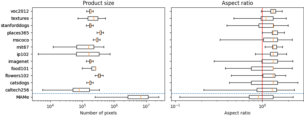
Figure 1: Product size and aspect ratio distribution over several datasets, both on log scale. The dashed horizontal blue line separates a sample of current image classification datasets, and the proposed MAMe dataset. The vertical red line at aspect ratio 1.0 shows the border between portrait (left side) and landscape (right side) images.

2 Related work

There are many visual challenge datasets in the current literature. There are however, very few containing images larger than 500x500 pixels, and with a significant variance in their aspect ratio. To illustrate that point we analyze a sample of popular datasets which satisfy three conditions we consider essential for attracting and generating high quality research:

• The dataset is publicly available.

• The dataset labels are reliable.

• The dataset has at least 100 instances per class.

The first requires data to be as public as possible, to reach the largest possible number of researchers. The second one excludes all datasets that contain labels not validated by humans or that have been crowd-labeled, as these may contain a significant amount of noise (and noise reduces the reliability of experimental results). The third enforces a minimum number of instances. We consider this a necessity for thorough research experimentation. We were nonetheless flexible in this regard, as some datasets of those analized contain some classes with less than 100 instances.

The sample analyzed contains the following 12 datasets: ImageNet 2012 [1], Food101 [25], IP102 [26], Places365 [27], Mit67 [28], Flower102 [29], CatsDogs [30], StanfordDogs [31], Textures [32], Caltech256 [33], Microsoft COCO [34] and Pascal VOC 2012 [35]. For each one we compute the product size (i.e., width multiplied by height) and aspect ratio (i.e., width divided by height) distributions. For the three datasets with more than 100,000 total samples (ImageNet 2012, Places365 and Microsoft COCO) we use a random sample of 100,000 images. Distributions for all 12 datasets can be seen in Figure 1.

In terms of number of pixels (left plot), current image classification datasets rarely contain images with more than 1 megapixel (MP). For reference purposes, none of the 12 datasets contain images bigger than 1,000 x 1,000 pixels, assuming unitary aspect ratio. This already indicates a significant bias in current research, and a mismatch with current technology, as popular image taking resolutions are well above that size. Obviously, there are datasets with images larger than 1 MP, but these are typically either private, unreliability labeled [22], or have very few instances per class [36]. In this context, as shown at the bottom of Figure 1, the MAMe dataset stands out, containing a large volume of reliable labeled HR images. In fact, all images in the Q1-Q3 interval of the MAMe dataset are bigger than the largest image found on all analyzed datasets. The mean image size for the MAMe dataset is 6.6MP (e.g., 2350x2350 in a squared image), one order of magnitude larger than all images contained in the analyzed datasets.

Regarding aspect ratio, the right plot of Figure 1 shows how the majority of images found in current datasets are landscape. All datasets have their median in the landscape side, only half of the datasets contain Q1 within the portrait side, and only 3 contain a significant amount of portrait images (Food101, CatsDogs and Caltech256). However, even these have their aspect ratio distribution clearly skewed towards landscape images (notice that the median is quite close to the third quartile on all three cases). In contrast, the proposed MAMe dataset has a balanced distribution, containing approximately the same number of portrait and landscape images. The aspect ratio distribution is also much wider than the other datasets, showing how the MAMe dataset contains infrequently wide and tall images.

3 The MAMe dataset

In this work we propose the Museum Artworks Medium dataset, abbreviated as the MAMe dataset. MAMe is an image classification dataset focused on the recognition of mediums in artworks and heritage held by museums (e.g., Oil on canvas, Bronze or Woodcut). Medium is a broad technical term used to describe several aspects of artworks [37]. On one hand, it can be used to describe the main physical components used for the creation of an artwork, such as Oil on canvas. However, medium can also refer to the technique used to produce the artwork. Engraving, for example, is the printed result of engraving a metal plate. Both of these interpretations of medium are freely used by museums to organize their collections.

As detailed in §1, the classes considered in the MAMe dataset comprise a wide variety of mediums according to both interpretations of the term. These can range from simple material aspects (e.g., Bronze, Silver or Gold) to complex, high-level techniques (e.g., Faience, Woodblock or Woven fabric). The variety of relevant features in MAMe requires both attention to detail and to the overall image structure. Meanwhile, the essence of art causes widely different artworks to share the same label. The degree of intra-class variance of MAMe is exemplified in Figure 2.

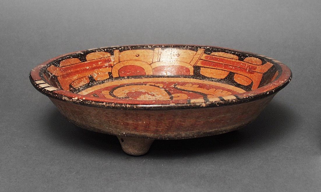
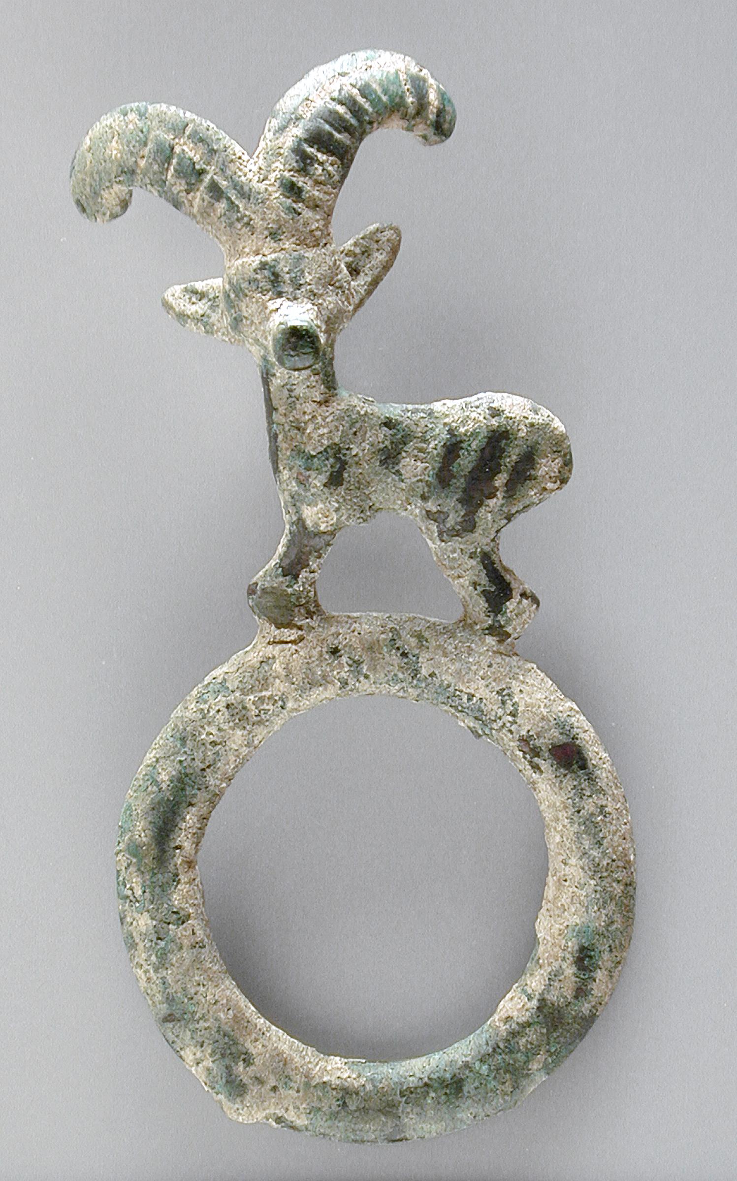
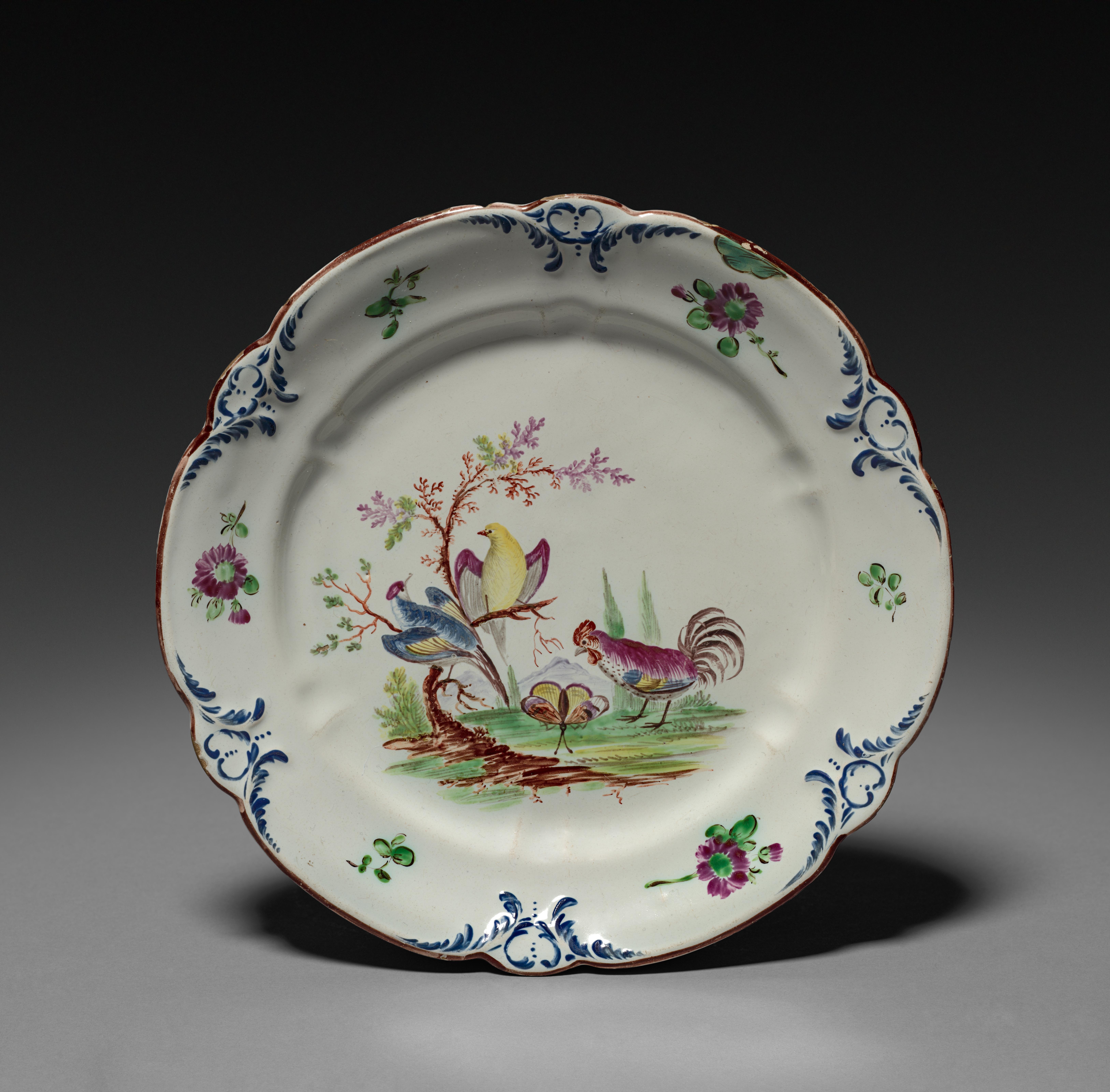
Figure 2: Example of intra-class variance. Images in the same row belong to the same medium class, but share few visual features. The first row belongs to Ceramic, the second row to Bronze and the third row to Faience.

3.1 Data acquisition

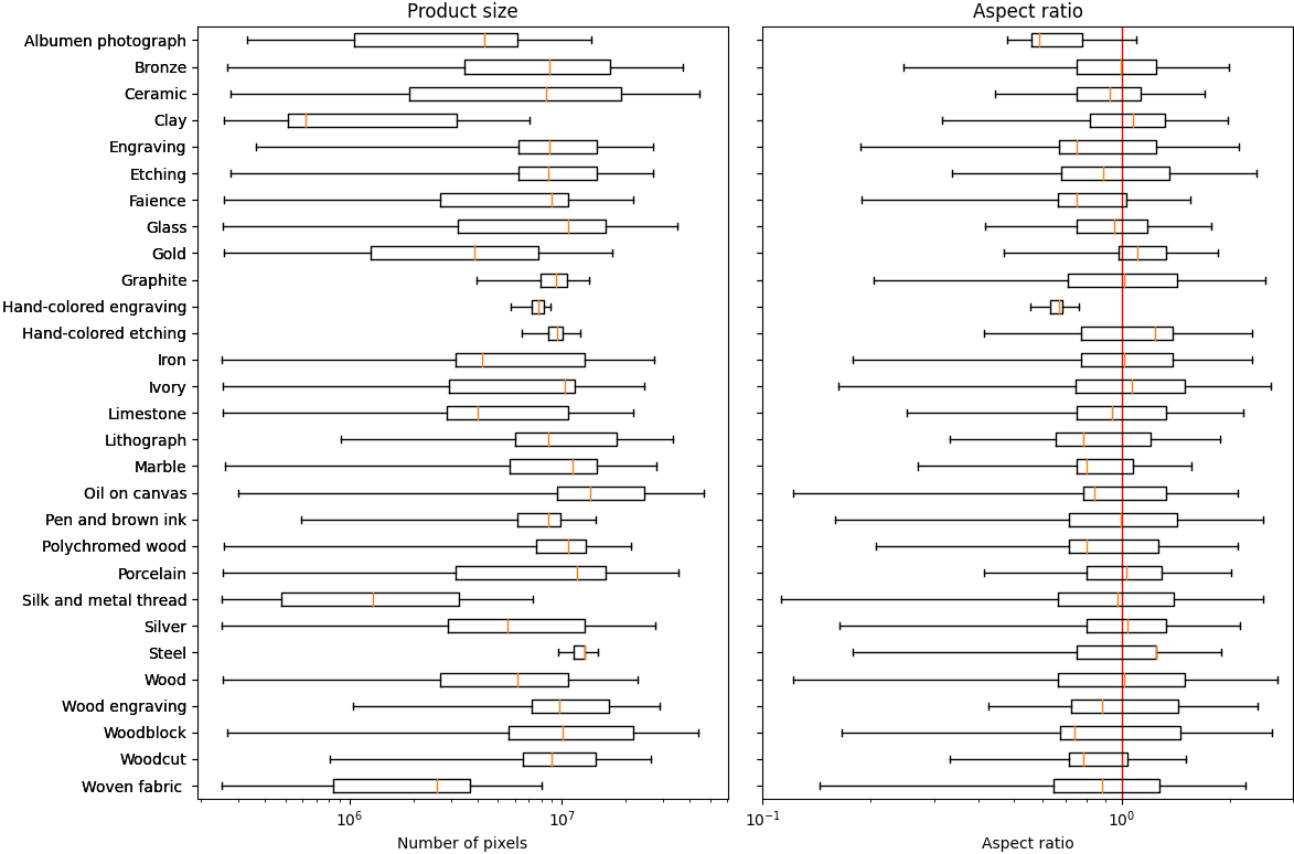
Figure 3: Product size and aspect ratio distribution over all classes of the MAMe dataset. Distributions are represented in box-plots, both of them on log scale. The vertical red line at aspect ratio 1.0 shows the border between portrait (left side) and landscape (right side) images.

In the past few years, museums around the world have been endorsing the policy of publicly releasing images of their heritage. Some of these museums release HR images under a CC0 license, allowing a free and unrestricted use of the data. We base our work on the data released by three museums. These were chosen because all three endorse the CC0 license, include a large number of images, provide accessible labels for them, and make it feasible to access their data in an automatized manner:

• The Metropolitan Museum of Art of New York (from now on the Met museum) [38].

• The Los Angeles County Museum of Art (from now on the Lacma museum) [39].

• The Cleveland Museum of Art (from now on the Cleveland museum) [40].

All three museums hold large artistic collections with a general scope, including artworks from all over the world, from very early cultures to recent ones. For accessing the data, the Cleveland museum publishes an API to automatically download images. Lacma and Met on the other hand provide access to their images only through their webpages. This implies an image-by-image download process, for which we built museum-specific crawlers. By these means we downloaded approximately 232,000 images from the Met museum, 26,000 from the Lacma museum and 32,000 from the Cleveland museum. From this data, we define the MAMe dataset, composed by an expertly-curated subset of the data. The final selection includes 37,407 images belonging to 29 classes. The class selection process was made following several technical criteria, including balance between museums (to avoid potential bias), balance and volume of class instances (to facilitate research), and image resolution (to enable HR exploration). Grey scale images were discarded. Significantly, museum images have a natural tendency towards VS (e.g., human sculptures tend to be tall, while paintings tend to be wide). Although we did not encouraged its presence, this natural feature is shown in the dataset statistics (see right plot of Figure 3).

Table 1: For each medium class within MAMe, distributions of instances among museums. The Met, Lacma and Cleveland museums are labeled as "Met", "Lac" and "Cle" respectively. Museum distributions are divided by data splits, into training, validation and test ("Train", "Val" and "Test" respectively). The last four columns show values aggregated for all data splits ("All"). The "Test" and "All" sections contain a 4th column indicating the total ("Total"). These values are not provided for "Train" and "Val" since these are constant (700 and 50 respectively).

Medium	Train			Val			Test				All
	Met	Lac	Cle	Met	Lac	Cle	Met	Lac	Cle	Total	Met	Lac	Cle	Total
Albumen photo	700	0	0	50	0	0	700	0	0	700	1450	0	0	1450
Bronze	234	233	233	16	17	17	233	233	234	700	483	483	484	1450
Ceramic	242	242	216	17	18	15	241	241	218	700	500	501	449	1450
Clay	695	5	0	49	1	0	310	2	1	313	1054	8	1	1063
Engraving	234	233	233	16	17	17	233	234	233	700	483	484	483	1450
Etching	234	233	233	16	17	17	233	234	233	700	483	484	483	1450
Faience	599	63	38	43	5	2	598	63	39	700	1240	131	79	1450
Glass	576	53	71	41	3	6	575	55	70	700	1192	111	147	1450
Gold	448	95	157	32	7	11	448	96	156	700	928	198	324	1450
Graphite	565	8	127	40	0	10	151	3	34	188	756	11	171	938
H-C engraving	30	641	29	3	45	2	14	300	14	328	47	986	45	1078
H-C etching	699	1	0	50	0	0	582	2	0	584	1331	3	0	1334
Iron	569	2	129	40	0	10	215	1	49	265	824	3	188	1015
Ivory	611	31	58	43	2	5	498	27	47	572	1152	60	110	1322
Limestone	593	56	51	42	5	3	591	56	53	700	1226	117	107	1450
Lithograph	277	147	276	19	11	20	276	148	276	700	572	306	572	1450
Marble	520	86	94	37	6	7	190	32	35	257	747	124	136	1007
Oil on canvas	265	171	264	18	12	20	264	172	264	700	547	355	548	1450
P&B ink	665	12	23	47	1	2	271	6	9	286	983	19	34	1036
Poly wood	525	59	116	37	4	9	281	32	62	375	843	95	187	1125
Porcelain	447	56	197	31	4	15	446	57	197	700	924	117	409	1450
S&M thread	680	0	20	48	0	2	92	1	2	95	820	1	24	845
Silver	452	81	167	32	5	13	450	83	167	700	934	169	347	1450
Steel	628	0	72	44	0	6	118	1	14	133	790	1	92	883
Wood	577	43	80	41	3	6	576	44	80	700	1194	90	166	1450
Wood engraving	410	15	275	29	1	20	211	9	141	361	650	25	436	1111
Woodblock	259	258	183	18	19	13	258	258	184	700	535	535	380	1450
Woodcut	417	51	232	30	3	17	416	52	232	700	863	106	481	1450
Woven fabric	658	3	39	46	0	4	656	5	39	700	1360	8	82	1450

3.2 Label mapping

All three museums (Met, Lacma and Cleveland) reported the medium used to represent their artworks as metadata. Unfortunately, there is not a unique ontology behind, as each museum uses a different level of detail and interpretation of medium. Some mediums are subtypes of another mediums. Some mediums are reported under different names. And some mediums are combinations of other mediums. Experts from the art domain grouped the medium metadata into coherent classes, following their professional understanding of artistic coherency and visual discriminability. Classes which could not be discriminated visually by a human without technical aid (e.g., a microscope) were discarded. The main expert criteria used to determine the classes are the following:

• Written coherency: Medium categories written in different forms refering to the same term are aggregated (e.g., Bronze and bronze)

• Terminology coherency: Medium categories which are considered to be analogous are aggregated (e.g., Ceramic and Pottery).

• Taxonomic coherency: Object belonging to the same parent medium are sometimes aggregated (e.g., Terracotta and Ceramic). Where technical criteria allows, medium subtypes are left as a separate class (e.g., Porcelain).

• Visual coherency: Medium categories which cannot be visually differentiated at plain sight are aggregated (e.g., Hard-paste porcelain and Soft-paste porcelain into Porcelain, Cotton and Linen into Woven fabric).

After enforcing a minimum amount of 850 samples per medium (adding up train, val and test), the MAMe dataset contains 29 different classes. These are shown in the left column of Table 1. Notice we made an exception with the Silk and metal thread medium, which only contains 845 samples. A detailed description of the nature of each class is provided in Table 2. Visual details on how to discriminate some of these classes are discussed in §5.

Table 2: Descriptions of the medium classes. Some descriptions are obtained from the museum sources [41].

Medium Description Albumen photograph Photographic prints on paper support. Paper is coated with egg white and silver nitrate, and exposed to sunlight in contact with a glass negative. Bronze Objects mainly made of bronze (cooper and tin alloy). Includes both polished and hammered bronze. Ceramic Includes pottery, stoneware, earthware and terracotta. It may include glazed, slip-painted or painted textures. Clay Objects made of clay or mud. In most cases the object has not been baked, or it has at very low temperatures. Engraving Intaglio printmaking process in which lines are cut into a metal plate in order to hold the ink. The plate can be made of copper or zinc. Etching Intaglio printmaking process in which lines or areas are incised using acid into a metal plate in order to hold the ink. The plate can be made of iron, copper, or zinc. Faience May contain egyptian faience (sintered quartz with a vitreous coating) or tin-glazed pottery. Glass Objects mainly made of glass (eg blown, or pressed). Stained glass windows are excluded. Gold Objects mainly made of gold. Includes polished gold, hammered gold and other surface textures. Graphite Drawings or sketches made with graphite lead on paper. Hand-colored engraving Engraving prints hand-colored after the printmaking process. Prints are colored using either watercolor or wash techniques. Hand-colored etching Etching prints hand-colored after the printmaking process. Prints are colored using either watercolor or wash techniques. Iron Objects mainly made of iron. Includes polished iron, hammered iron and other surface textures. Ivory Objects made mainly of ivory (elephant or walrus tusks). Includes watercolor on ivory miniature portraits (medallions). Limestone Objects mainly made of limestone, a sedimentary rock mainly composed by calcium carbonate. Lithograph Planographic printmaking process in which a design is drawn onto a flat stone (or prepared metal plate, usually zinc or aluminum) and affixed by means of a chemical reaction. May contain lithographic offset prints and hand-colored monochrome lithographs. Marble Objects mainly made of marble, a metamorphic rock composed of calcite or dolomite. Oil on canvas Fabric streched into frame (stretcher bar), with a preparation layer (or ground layer) painted with linseed oil and pigment. Pen and brown ink Drawings or sketches on paper, mainly made in brown ink (either with a dip pen, a fountain pen or a brush). Can be supplemented by other procedures such as wash (brown or black ink) or dry media. Some artworks may contain aged iron gall ink, or other similar brown inks such as bister or sepia ink. Polychromed wood Objects made of painted wood. Includes three-dimensional objects and painted surfaces, such as panel painting (oil on wood or tempera on wood). Porcelain A type of ceramic composed by quartz, feldspar and kaoli cooked at high temperatures. May contain soft-past porcelain. Silk and metal thread Woven fabric objects made of silk with metallic threads, typically forming an embroidery. Silver Objects mainly made of silver. Includes both polished and hammered silver. Steel Objects mainly made of steel (alloy of iron with carbon). Wood Non polychromed wood objects. Inlcudes several wood types such as oak, boxwood or limewood. Wood engraving A type of woodcut printmaking process characteristic for using a block cut along the end-grain. Woodblock A type of woodcut printmaking process typically used by oriental cultures. This type of woodcut is carved along the wood grain and uses a different block for each color printed. Woodcut The oldest form of printmaking. Relief process in which knives and other tools are used to carve a design into the surface of a wooden block. The raised areas that remain after the block has been cut are inked and printed, while the recessed areas that are cut away do not retain ink, and will remain blank in the final print. Woven fabric Fabric objects woven with a loom. Includes linen, cotton, silk and others. Fabrics appear in several forms such as plain fabrics, embroideries or printed fabrics.

3.3 Dataset details

The MAMe dataset is publicly available . The site provides access to all the original images, and a CSV file with metadata for each of them. This metadata includes the following information:

• the image filename

• the medium of the artwork (i.e., the classification label)

• the museum from where the image was obtained

• the artwork ID given by the museum

• the data split of the instance (i.e., train, validation or test set)

• the width of the image

• the height of the image

• the product size of the image (i.e., width multiplied by height)

• the aspect ratio of the image (i.e., width divided by height)

The dataset contains 29 medium classes. Each class is composed by at least 850 images and, at most 1,450. Each class contains 700 images for training, 50 images for validation and a variable amount of images for the test set (i.e., the test set is unbalanced). The minimum amount of instances in the test set is 100 (except for Silk and metal thread with 95) and the maximum is 700. In total, the MAMe dataset is composed by 37,407 HR images. All images in the MAMe dataset have, at least, a resolution of 0.25MP, equivalent to a squared image of 500x500 pixels. The mean resolution is around 10.3MP, corresponding to an image of more than 3,200x3,200 pixels, and the greatest image has more than 370MP corresponding to an image of 32,683x11,412 pixels (check Figure 1). The 37,407 images are divided in subsets as follows: 20,300 images for training and 1,450 images for validation and 15,657 for test. Of those, 24,911 images originate from the Met museum, 5,531 images from the Lacma museum and 6,965 images from the Cleveland museum. An effort was made to keep the data coming from the different museums as balanced as possible, to minimize the possibility of potential biases generated by the nature of artworks and the image taking particularities of each museum. The exact distributions of images per museum, class and data split are shown in Table 1. To assess the internal balance of MAMe with regards to HR and VS features, Figure 3 shows the product size and aspect ratio distributions for each medium class. Besides a few classes with particularly narrow or skewed distributions, most of the categories include a wide variety of product sizes and aspect ratios.

4 Baselines and Experiments

This section introduces and evaluates both a set of baseline models and a set of hypothesis. The purpose of baselines is to illustrate how the task proposed is coherently constructed (i.e., solvable) and worth receiving the attention of researchers. To this end, we employ prototypical solutions from the literature that provide good results on other challenges, and report their performance on the MAMe dataset.

Figure 4: Visualization of the different MAMe data types, exemplified for one particular instance. FS stands for fixed shape and VS for variable shape. R stands for resolution and A for axis.

Additionally, to highlight differences of high resolution (HR) and variable shape (VS) properties w.r.t. low resolution (LR) and fixed shape (FS) in the context of MAMe, we perform a set of experiments. These are designed to evaluate the following hypothesis:

Hypothesis 1 (H₁):

MAMe benefits from HR data w.r.t. LR data.

Hypothesis 2 (H₂):

MAMe benefits from VS data w.r.t. FS data.

Hypothesis 3 (H₃):

MAMe benefits from information gain w.r.t. only resolution gain.

All baseline models, hypothesis experiments and the code needed to replicate results are publicly available .

4.1 MAMe data types

Most of current solutions in the literature use squared images to feed their models, that is images with a fixed shape. Additionally, these squared images are typically of low resolution. Resolutions used are diverse, but the most common is 256x256 pixels, corresponding to a total amount of 65,536 pixels. For referencing purposes, we use this data type as a starting point and we call it R65k-FS. For comparison purposes, we use a second data type using the same resolution (i.e., same amount of total pixels) but keeping the original aspect ratio of the image, that is with the VS property. This second data type is called R65k-VS. We also produce the HR versions of these two data type. These HR versions contain a total of 360,000 pixels. They are the R360k-FS and the R360k-VS version. Notice that R360k-FS corresponds exactly to an squared image of 600x600 pixels, while R360k-VS contains images of variable shape but fixed number of pixels. See Figure 4 for an illustration of all data types used.

The final list of data types used in this section is as follows:

• R65k-FS: images are downsampled to 256 x 256 pixels, corresponding to an image size of 65,536 pixels.

• R65k-VS: the original aspect ratio is maintained forcing the total number of pixels to 65,536.

• R360k-FS: images are resized to 600 x 600 pixels (360,000 pixels)

• R360k-VS: images are rescaled to a total number of pixels to 360,000, maintaining the original aspect ratio.

4.2 Training configurations

In this work we use very well-known architectures: VGG [10], ResNet [3], DenseNet [23] and EfficientNet [16]. The specific architecture versions that we use are the following:

• VGG11 (configuration A)

• VGG16 (configuration D)

• ResNet18

• ResNet50

• EfficientNet-B0

• EfficientNet-B3

• DenseNet121

Our baselines and experiments use several types of input processing. This is divided into two main components: data processing and data augmentation. The first refers to all image transformations required to obtain each data type (according to subsection 4.1), while the second provides regularization during the training process. The data augmentation is independent of the data type, and is defined as follows:

1. Random rotation of the image from [-30, 30] degrees.

2. Random crop of (0.875 x width, 0.875 x height) pixels. Width and height refer to current dimensions at this point of the processing.

3. Random horizontal flip with 50% chance.

As a final step, images are normalized to have values in the range [0, 1] and standardized with $\mu=0.5$ and $\sigma=0.5$ (same value for all three channels). Notice that during validation, the data augmentation is adapted. In this phase, steps 1 and 3 are avoided and, step 2 does a center crop instead of random one.

We use the AMSGrad optimizer [42] for all the baselines and experiments, a variant of the original Adam optimizer [43]. Batch sizes and learning rates are optimized for each training, considering memory limitations, training speed and learning convergence. Executions are conducted in a single computing node of the CTE-Power9 cluster at the Barcelona Supercomputing Center, with the following characteristics:

• 2 Sockets x IBM Power9 8335-GTH @ 2.4GHz (20 cores and 4 threads/core, total 160 threads).

• 4 x GPU NVIDIA V100 (Volta) with 16GB HBM2.

4.3 Baselines performance

To show the feasibility and evaluate the difficulty of the MAMe task, we introduce a set of baseline models. Their purpose is to reach the best possible performance using current prototypical solutions. To that end, we employ the following CNN architectures: VGG11, VGG16, ResNet18, ResNet50, EfficientNet-B0, EfficientNet-B3 and DenseNet121. We train these using the four MAMe data types explained in subsection 4.2. Due to memory limitations, we only use a subset of architectures on the R360k data type: VGG11, ResNet18, EfficientNet-B0 and EfficientNet-B3. All baselines are trained on top of the corresponding ImageNet pre-trained models . Top 10 baseline results are shown in Table 4. These reported results correspond to the mean per class test accuracy using the models achieving minimum validation loss.

Table 3: Top 10 baseline results for the MAMe dataset. Notice the prevalence of high resolution to a great extent.

Architecture	Resolution	Shape	Accuracy
EfficientNet-B3	R360k	FS	88.95%
EfficientNet-B0	R360k	FS	88.25%
Resnet18	R360k	FS	88.15%
VGG11	R360k	VS	85.42%
EfficientNet-B3	R65k	FS	85.11%
VGG11	R360k	FS	85.04%
Resnet18	R360k	VS	84.59%
Resnet50	R65k	FS	84.29%
Resnet50	R65k	VS	84.07%
EfficientNet-B0	R65k	FS	83.73%

Table 4: Experiment results for H₁ (more resolution is better) and H₂ (less deformation is better) hypotheses. H₁ is assessed vertically (same shape policy, variable resolution), while H₂ is assessed horizontally (same resolution, variable shape policy).

	FS	VS	Architecture
R65k	81.35%	81.39%	VGG11
	81.20%	81.21%	VGG16
	83.33%	82.66%	ResNet18
	84.29%	84.07%	ResNet50
	73.14%	76.06%	DenseNet121
	83.73%	82.38%	EfficientNet-B0
	85.11%	83.48%	EfficientNet-B3
R360k	85.04%	85.42%	VGG11
	88.15%	84.59%	ResNet18
	88.25%	79.11%	EfficientNet-B0
	88.95%	80.04%	EfficientNet-B3

After training multiple models with combinations of seven architectures and four MAMe data types, finetuning each of the training models to optimize performance and using pre-trained models from ImageNet, most models achieve accuracies above 80%. The maximum 88.95% accuracy is obtained by the EfficientNet-B3 architecture on the R360k-FS data type. These results show that, indeed, the MAMe task is solvable. It also clearly illustrates the benefits of using higher resolutions, as the top 4 models are based on R360k data types. On the other hand, it seems that models are not properly exploiting the VS property, as only VGG11 manages to be in the top 4 with that shape policy. Next, let us assess the relevance of these properties in further detail.

4.4 Hypothesis evaluation

In this section we aim to validate the three hypothesis introduced in section 4. Our first hypothesis is H₁: MAMe benefits from HR data w.r.t. LR data. Since HR contains extra information that is not present in LR data, this hypothesis aims to measure to which degree is this additional information relevant for improving performance on MAMe.

To test H₁ we train a set of models using R65k-FS and R360k-FS MAMe data types, where the only difference is the resolution of images. Notice both data types share the same proportional distortion w.r.t. the original shape of images. We do the same experiment using variable shape (i.e., R65k-VS and R360k-VS data types). In this case the only difference is the resolution of images because there is no distortion added to the aspect ratio. The architectures used for validating this hypothesis are VGG11, ResNet18, EfficientNet-B0 and EfficientNet-B3. We use this subset of shallow architectures due to the high-memory requirements when using R360k data. The models are trained starting from their corresponding ImageNet pre-trained models. Results are shown in Table 4 and Table 6.

Table 5: Difference in performance between models trained using R65k and R360k data. This results are used to validate hypothesis H₁.

	FS	VS	Architecture
R65k to R360k	+3.69%	+4.03%	VGG11
	+4.82%	+1.93%	ResNet18
	+4.52%	-3.27%	EfficientNet-B0
	+3.84%	-3.44%	EfficientNet-B3

Table 6: Difference in performance between models trained using FS and VS data. This results are used to validate hypothesis H₂.

	FS to VS	Architecture
R65k	+0.04%	VGG11
	+0.01%	VGG16
	-0.67%	ResNet18
	-0.22%	ResNet50
	+2.92%	DenseNet121
	-1.35%	EfficientNet-B0
	-1.63%	EfficientNet-B3
R360k	+0.38%	VGG11
	-3.56%	ResNet18
	-9.14%	EfficientNet-B0
	-8.91%	EfficientNet-B3

H₁ is validated for 6 out of 8 comparison pairs. In these, the models trained on HR data (i.e., R360k) achieve a boost in performance around 4%. This happens for all four architectures tested (VGG11, ResNet18 and the EfficientNet variants). Noticeably, the two cases where using HR data does not yield benefits (and instead degrades around 3%) are VS settings using the EfficientNet architectures. This phenomenon will be further studied and discussed next, when we assess the validity of H₂ hypothesis.

Let us now consider the second hypothesis H₂: MAMe benefits from VS data w.r.t. FS data. Since the FS property deforms the original image adding some distortion, this hypothesis aims to measure to which degree is this deformation relevant for performance on MAMe. For this purpose we compare models which have the same resolution and only differ in shape; we compare R65k-FS with R65k-VS, and R360k-FS with R360k-VS. The architectures used for the R65k comparison are all architectures listed in section 4.2, but architectures used in the R360k comparison are a subset of them due to high-memory requirements: VGG11, ResNet18, EfficientNet-B0 and EfficientNet-B3. All models are trained starting from ImageNet pre-trained models. Results are shown in Table 4 and Table 6.

With regards to H₂, results do not fully validate nor reject it. Prototypical architectures do not adequately take advantage of the VS property, either by obtaining insignificant accuracy variations (VGG11, VGG16, ResNet18-R65k and ResNet50) or even producing a negative effect on performance due to VS (ResNet18-R360k, EfficientNet-B0 and EfficientNet-B3). Only for the case of DenseNet121 on R65k data, performance increases when moving from FS to VS. Overall, results are inconclusive regarding this second hypothesis H₂.

The experiments with regards to H₂ are affected by the padding. To process images of VS in a single batch, it is required that they all have exactly the same shape for computational purposes. Doing so without changing the shape implies the addition of padding pixels, that is, non-informative values (typically zeros) that are used to uniform batch shape. However, existing architectures do not differentiate padding pixels from image pixels, counting as noise during the training process. Remarkably, this noise increases considerably under a HR setting, where the absolute amount of padding pixels increases. In this regard, some preliminary experiments conducted on a previous version of the MAMe dataset [44] indicate that reducing padding in a VS setting can yield to accuracy improvements between 3% and 5%.

As illustrated in the results of the H₁, on the MAMe dataset a gain in resolution implies a gain in performance. However, as suggested by Sandler et. al. [24], such increase in performance may be due to an increase of the input size or due to an increase of the internal representation of the model. In their publication [24], they evaluate the impact of these two factors with an experiment on the ImageNet dataset. This experiment consist on comparing information gain against resolution gain, by assessing pairs of models trained with images of same resolution but different amount of information:

• Full-information images: Images that are downsampled to a target resolution and contain their corresponding amount of information.

• Capped-information images: Images that are, first, downsampled to a 224x224 resolution and, second, upsampled to a larger target resolution (Bilinear interpolation). Notice that such image will be of same resolution than its corresponding full-information image, but it will contain less original information.

Full-information images increase the model internal representation and the input information, while capped-information images increase the model internal representation as well, but do not increase the input information. By comparing performances using both, we can isolate the impact of the input information when increasing the image resolution.

To evaluate the impact of image information gain on the MAMe dataset, we formulated our third hypothesis H₃: MAMe benefits from information gain w.r.t. only resolution gain. While this hypothesis is rejected in ImageNet according to [24], next we test if this is also the case for MAMe. To conduct this experiment, we train FS models on VGG11 and ResNet18 architectures using the following target resolutions: 50k, 90k, 160k, 250k and 360k pixels. These correspond to squared image widths of 224, 300, 400, 500 and 600 pixels. For each target resolution, we use full-information and capped-information images. Notice both full-information image and capped-information image are equivalent for the image width of 224 pixels. Results are shown in Figure 5.

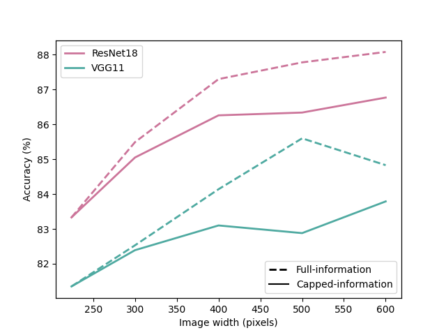
Figure 5: Results when training VGG11 and ResNet18 architectures using full-information (downsampled from original) and capped-information (upsampled from 224) images. Target resolutions used are the ones corresponding to image widths of 224, 300, 400, 500 and 600 pixels. Both settings improve with size, indicating that both resolution and information gain contribute to better performances in MAMe. Notice the experiment at 224 width is not capped information.

Results obtained by Sandler et. al. [24] on ImageNet dataset [1] indicate that there is no gain in performance due to information gain (see their Figure 2b). Indeed, improvement in their experiments is only caused by the use of larger model internal representations. In the MAMe dataset, this very same experiment shows that improvement occurs for both reasons. Increasing the model internal representation (capped-information) entails some consistent improvement in performance. However, performance is further boosted when also increasing the information (full-information). These results suggest the third hypothesis holds for the MAMe dataset, and further highlights the inherent differences between MAMe and ImageNet.

5 Expert and explainability analysis of MAMe

The domain of artworks and heritage is defined by human technology, skill and creativity. Art experts can identify a set of visual queues useful for the characterization of art, but remains to be seen if AI models learn these same features. To analyze these features in the context of the MAMe dataset, we analyze several medium classes from an expert point of view and perform explainability experiments. We perform explainability on two models trained from scratch with two data types. On one hand, the R65k-FS is used to characterize a low resolution and fixed shape setting (LR&FS). On the other hand, to highlight a high resolution and variable shape (HR&VS) we introduce a new data type version: the A500-VS. This new HR&VS version ensures a minimum size of 500 pixels per axis, preserving the original aspect ratio, as illustrated in Figure 4. The main reason for using A500-VS instead of R360k-VS is to facilitate visualization. In this case we use the architecture most widely used for this kind of experiments, the VGG [10]. In our case, we use the shallow version VGG11 to handle the high-memory requirements of A500-VS. By understanding the focus of the LR&FS and HR&VS models, we can detect the most relevant class features according to them. These explanations allow experts to assess the consistence of the decisions made, and detect the potential existence of bias. Finally, comparison between LR&FS and HR&VS explanations offers an additional exploration about the impact of HR and VS properties in the MAMe dataset.

5.1 Layer-wise relevance propagation

In our analysis we use post-hoc interpretability [45]: Methods used to interpret the model predictions once the model has been trained. For image classification, a widely used visual explanation are the saliency methods. These methods use saliency maps to show the features on the image that contribute to a prediction. In other words, which pixels in the input image are important for the classification task. Among this family of methods [46, 47, 48, 49, 50], we use Layer-wise Relevance Propagation (LRP) [51] which has been used in different fields performing meaningful explanations [52, 53, 54, 55]. The LRP technique backpropagates the output prediction to the input image, by computing the contribution of each neuron w.r.t. the output prediction. That is, effectively mapping the relevance of an specific class into the pixels of the input image.

Although different LRP rules have been proposed, we implement the recent Composite LRP [56]. This technique proposes to combine different propagation rules depending on the depth of the layer. Our Composite LRP makes use of LRP$-0$ for last layers, LRP$-\epsilon$ ($\epsilon=0.25$) and LRP$-\gamma$ ($\gamma=0.25$) for intermediate layers, and LRP$-z^{B}$ for the first layer of the network, as illustrated in Figure 6.

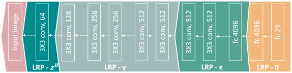
Figure 6: LRP rules applied to each layer of the VGG11 network.

So, given an image $I$ and a specific class $c$, the Composite LRP produces an explanation heatmap $E_{I,c}$. The color convention for this heatmap is as follows: red is used for positive contributions, while blue indicates negative contributions. That means, the red areas are considered descriptive patterns of the given class by the model. Meanwhile, the blue areas are considered typical patterns of other classes.

We perform two types of LRP analysis, one for the correctly predicted images, and another one for the incorrectly predicted images. In case of correctly predicting the medium $m$, we produce its corresponding explanation heatmap $E_{I,m}$. In this case, the red areas of the heatmap correspond to descriptive patterns of the predicted medium $m$ and blue areas to descriptive patterns of the rest of mediums. In the case of incorrectly predicted images, we computed the explanation as the difference between two heatmaps. The one associated to the real medium $r$, minus the one associated to the predicted medium $p$:

$$E_{I,r,p}=E_{I,r}-E_{I,p}$$ (1)

This difference allows to remove the contributions to the predicted class, focusing on the features that contribute to the real class. In this visualization, the red areas will be considered typical patterns of the real class but not of the predicted class, while blue areas will be considered typical patterns of other classes (most of them probably from the predicted class).

5.2 Best and worst performances

First, let us focus on the classes that are best and worst recognized by the two models trained on the two versions of the MAMe dataset introduced before:

• The model trained from scratch on images of LR&FS (R65k-FS), using the VGG11 architecture.

• The model trained from scratch on images of HR&VS (A500-VS), using the VGG11 architecture.

Among the best ones we can count Albumen photograph, Gold and Graphite. In the case of Albumen photograph, we only have one type of photographic technique in the MAMe dataset, making these images easily distinguishable from other cultural assets. The class Gold is a similar case, since the golden color differentiates it from other metals, despite having other objects in the dataset of similar shapes. Lastly, Graphite is a drawing technique that uses similar grey tones with metallic brightness and smooth strokes that usually end at the edge of the paper. These characteristics help avoiding confusions between Graphite and Lithograph, which in some cases may be similar. For these reasons these mediums are easily recognizable, not only for the LR&FS and HR&VS model, but also for human experts.

On the other side of the spectrum we have the classes that are most poorly recognized by these two models. These are Woven fabric, Polychromed wood, Etching and Silk and metal thread. These classes are hard to predict because they belong to fine-grained groups of classes, with many common features. Following expert guidelines we identify the following fine-grained groups. These are discussed in further detail next.

• Prints: Etching, Engraving, Wood engraving, Woodcut, Woodblock, Lithograph

• Fabrics: Woven fabric, Silk and metal thread

• Paintings: Polychromed Wood, Oil on canvas

5.2.1 Prints group

From an expert perspective, the most complex fine-grained group is Prints. They are hard to differentiate because they may look very similar, despite having been printed through different procedures. Common clues used by experts for their discrimination include the definition of lines, the appearance of strokes, the homogeneity of shadows or color areas, as well as the intensity of blacks. A common feature used to identify different kinds of prints is the platemark. Platemark is the rectangular ridge created in the paper of a print by the edge of an intaglio plate. These marks can be essential for the discrimination of certain print classes: While both Engraving or Wood engraving have very defined lines and grid patterns, they can be told apart through platemarks since these only appear on the edges of an Engraving. Within the same group Prints, Woodblocks are distinguishable from the rest because of their oriental aesthetics. They are usually colored prints that use one block for each ink. As a result, colors sometimes overlap, and/or leave gaps in the outlines. However, this last characteristic is also found on other colored prints like Lithographs or Woodcuts. One last example to illustrate the complexity within Prints could be Etching and Engraving. These two techniques are very similar, having the same aforementioned platemarks and often the same grid patterns in their printed areas. In this case, experts need to appreciate the contours of the lines for differentiation. They are more vibrant and less defined in Etchings, and they have convex edges for Engravings.

In sight of the expert knowledge, image resolution seems key to properly detect main discriminating patterns. In some cases, even our HR&VS images seem to fall short in resolution (e.g., grid patterns are lost). As an example, Figure 7 shows a rectangular region of an Engraving in original resolution (left side) and in HR&VS (right side). Zoomed area shows the central figure of the print, a fisherman. If we focus on the clothes, we can clearly perceive the characteristic grid pattern of an Engraving in the original resolution image, but these are lost on the HR&VS image, where the grid become a gray blur due to the interpolation when resizing the image.

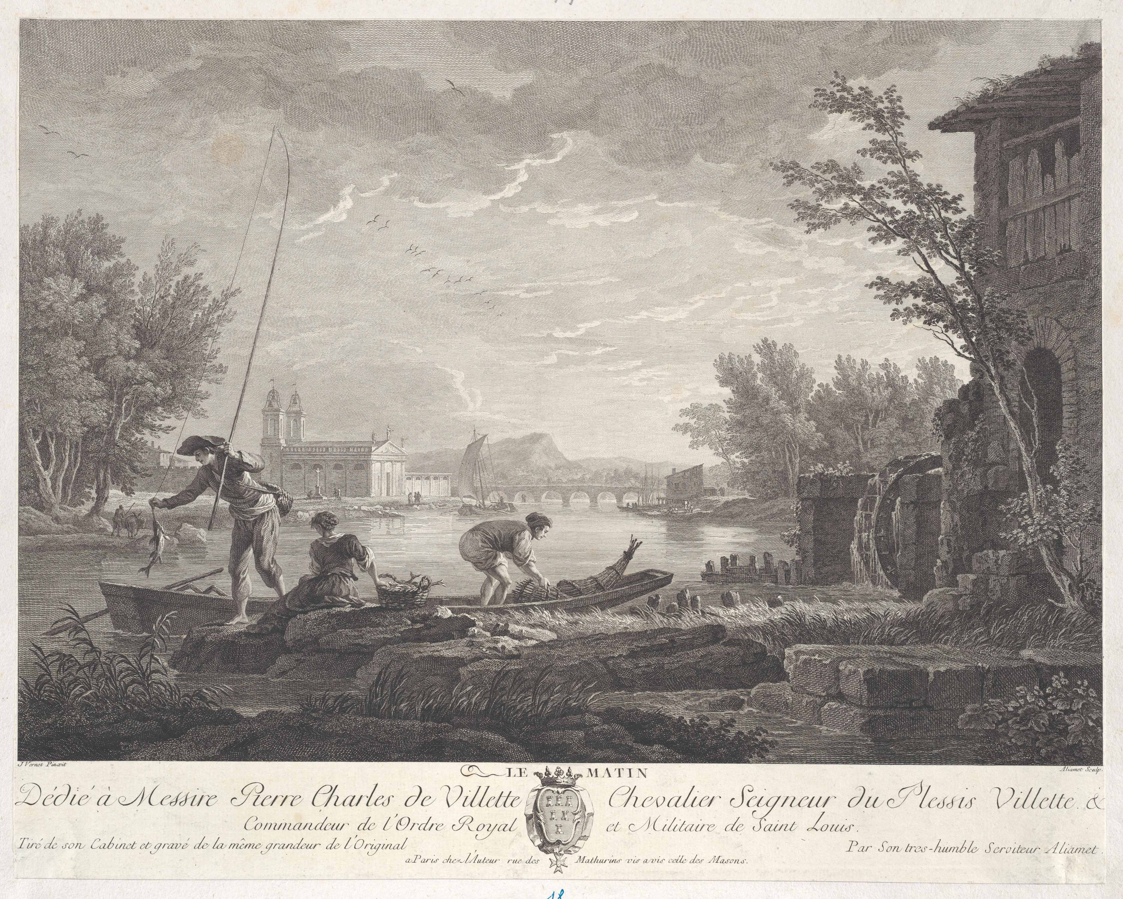
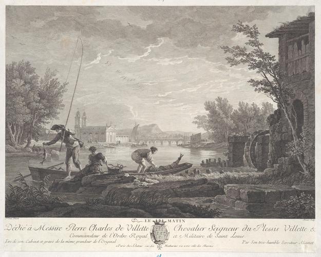
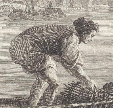
Figure 7: Example of an Engraving artwork at its original size (left side) and HR&VS (right side). The second row shows the same zoomed area for both images, where the grid pattern can only be perceived on the original resolution (left).
Met museum: 53.600.1616

5.2.2 Fabrics group

The second group of fine-grained classes is Fabrics. To discriminate these with total confidence it is necessary to identify the fibers using microscopy techniques. This condition motivated the aggregation of several classes within Woven fabric (e.g., linen, cotton, silk and others). Nonetheless, one particular type of woven fabric can be visually recognized without the aid of external machinery. That is Silk and metal thread, which are clearly distinguishable from other textile fibers due to the glitter of metallic threads.

Figure 8: Example of Silk and metal thread in HR&VS (left) and LR&FS (right). The brightness of the metal threads is visible in both cases.
Met museum: 2002.494.278

In Figure 8, we can see the metallic glitter in LR&FS and HR&VS images (more clearly on the latter). However, both models have been unable to properly discriminate these two classes. If the model does not detect this feature, it will learn other patterns for differentiating these two classes, such as ornamental motifs. However, this is not a reliable discriminatory feature and, therefore, it could be a source of error. We performed explainability experiments on several images and found cases where the model focuses on the ornamental motifs as shown in Figure 9.

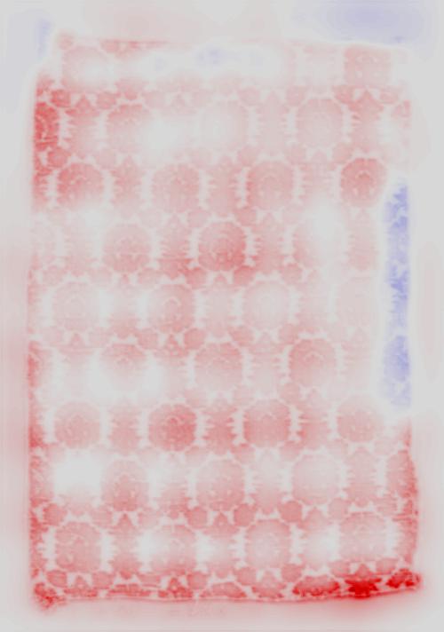
Figure 9: Example of Silk and metal thread in HR&VS (left) and its LRP explanation (right). The ornamental motifs (red zones) have positively contributed to the Silk and metal thread class classification.
Met museum: 2002.494.366

5.2.3 Paintings group

The third group of fine-grained classes is Paintings. This group contains two classes: Polychromed wood and Oil on canvas. The main reason why these classes are hard to differentiate is because Polychromed wood contains the subclass panel paintings (i.e., a painting on a flat panel made of wood), which are similar to Oil on canvas. Both, Polychromed wood panel paintings and Oil on canvas, hide the support behind the paint layer, complicating the identification of the support material (fabric or wood). In this context, experts pay attention to cracks, leaks or textures that may be characteristic of the support below the paint. Nonetheless, these features may not be properly visible in a single LR&FS or HR&VS images.

There are several Oil on canvas images that are incorrectly predicted as Polychromed wood, both in LR&FS and in HR&VS. It makes sense from an expert point of view since, in several HR&VS images, it is impossible to appreciate any detail that may suggest whether the support is wood or fabric, forcing the model to guess the class based on alternative patterns that may be misleading. For example, one of the key properties that identify an Oil on canvas is the canvas weave pattern. Unfortunately, this seems to be visible only on a few HR&VS images. Within this work, art experts reviewed around 1̃50 images where the two models failed to discriminate between Oil on canvas and Polychromed wood, and considered that they could only see the canvas weave pattern in approximately 5% of the HR&VS images. In Figure 10, we show an example of an Oil on canvas image where it is possible to perceive the canvas weave pattern. Although this pattern is present in the HR&VS image but not in the LR&FS image, both models misclassified this example, indicating that the HR&VS model does not pay attention to this property.

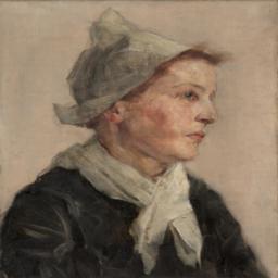
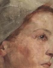
Figure 10: Example of Oil on canvas in HR&VS (left side) and LR&FS (right side). The second row shows the zoomed area where it is possible to perceive the canvas wave pattern in the HR&VS but not in the LR&FS image.
Cleveland museum: 1943.324

5.3 LR&FS and HR&VS comparison

In this section we explore the classes with greatest difference in accuracy between the two models we are exploring: the one trained on LR&FS images and the one trained on HR&VS images. In order, these classes are Lithograph (+16.28% gain by HR&VS), Bronze (+15.71% gain by HR&VS) and Engraving (+14.85% gain by HR&VS). Lithograph and Engraving are within the Prints group which, as reviewed in §5.2.1, can benefit from more detailed inputs for their discrimination. The third, Bronze is a material which can be easily differentiated by a human expert.

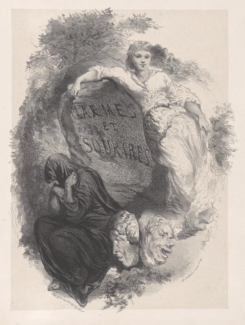
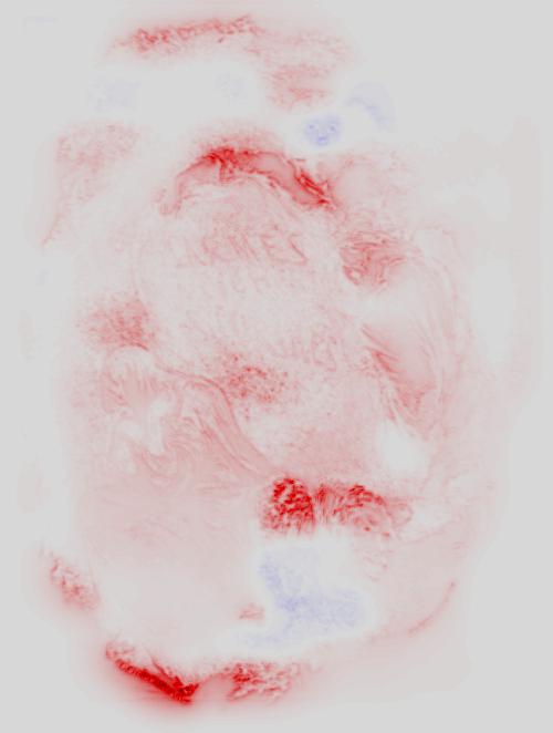
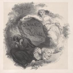
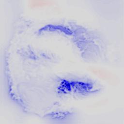
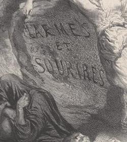
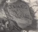
Figure 11: Lithograph example in HR&VS and LR&FS. There is a top side and a bottom side divided by an horizontal black line. Top shows the image in HR&VS and its corresponding LRP explanation. Both models focus on the general texture for their predictions, although LR&FS mispredicts Wood engraving. Bottom side shows a zoomed area of the print in HR&VS (left) and LR&FS (right). In here we can see the granular texture of the surface typical of this class in HR&VS, but not in LR&FS.
Met museum: 49.21.53

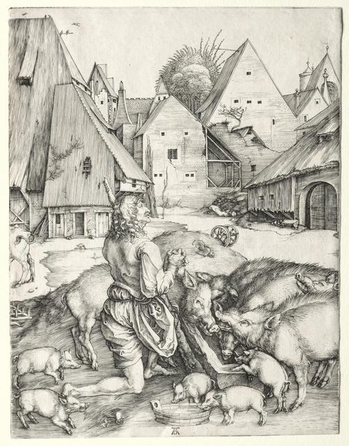
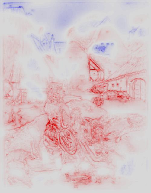
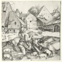
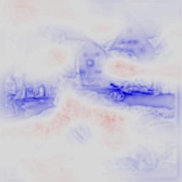
Figure 12: Engraving example in HR&VS and LR&FS and its corresponding LRP explanations. Check how the contours of the figures positively contribute to the prediction of the class in HR&VS format. LR&FS loses most these details, and mispredicts it as Wood engraving.
Cleveland museum: 1958.105

Let us start with the case of Lithograph. Figure 11 shows a representative example of this class, illustrating both the input and the LRP for the HR&VS and LR&FS models. Both models focus on the overall texture of the image (the LRP relevance is spread throughout the image), but with different impacts on the prediction: it represents negative evidence for LR&FS (which ends up in mispredicting the class Wood engraving) but positive evidence for HR&VS. Experts highlight the relevance of the texture of Lithographs for their discrimination from other similar classes like Woodblock, Hand-colored etching, Wood engraving or Hand-colored engraving. Lithographs contain a granular texture that is not present on the other classes, but this texture is only visible at a certain resolution, as shown in the zoomed tombstone at the bottom of Figure 11. This LRP results indicate that the HR&VS model follows a similar strategy to distinguish Lithograph from other classes, successfully recognizing the textures from prints and properly interpreting them for the final prediction. The LR&FS model, unable to recognize the granular texture, fails at finding relevant features towards Lithograph.

Figure 12 shows an example of the Engraving class, which has been correctly predicted by the HR&VS but not by the LR&FS (mispredicted as Wood engraving). The Figure contains the entire image and its corresponding LRP explanation for both, HR&VS and LR&FS, which target really different aspects of the print: While HR&VS focuses on the contours of the print figures, LR&FS does not. According to experts, these figure contours are dark areas that encode essential information for discriminating the mediums within the Prints group. Contours can only be properly inspected at high resolutions. Some of this information is retained in HR&VS images, as reviewed by experts. Meanwhile LR&FS images lose all relevant details.

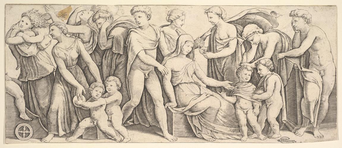
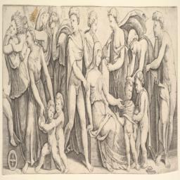
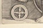
Figure 13: First row shows an Engraving in HR&VS and LR&FS. Notice the deformation of the latter. Second row shows a zoomed area, to illustrate how the grid lines become blurred in the LR&FS version.
Met museum: 17.3.3169

As mentioned in subsection 5.2.1, another property to distinguish printing techniques is the grid pattern. Although in some cases it can only be perceived in the original resolution image, some HR&VS image retain this information. However, this is always lost in the LR&FS images. On top of that, the image distortion produced by the shape variation of LR&FS images forces the grid lines closer in one axis (unpredictably, as it depends on the original image aspect ratio), complicating its identification. As an example of that, Figure 13 shows an Engraving image in HR&VS and LR&FS format, where the latter shows a great image distortion. It also shows a zoomed area, highlighting the differences in the grid pattern.

The last case we consider in this section is the third class with the biggest difference in performance. This is the Bronze class, which includes a great variety of objects (e.g., sculptures, ornaments), but specially coins. One of the main reasons why there are so many coins inside the Bronze class is that, historically, Bronze has been a usual alloy used to mint coins. One of the main characteristics of a coin is its circular shape. However, this property is lost when deforming the image due to the uniformization of aspect ratio inherent to LR&FS inputs. The lack of a uniform shape of coins has a negative impact on their recognition, which is not found on the HR&VS model. A clear example of this can be observed in Figure 14. The corresponding LRP explanations show, on one side, the positive impact of the rounded coin contour for the HR&VS image and, on the other side, the negative impact of the deformed coin for the prediction of the LR&FS image. This particular LR&FS example is mispredicted with Steel, which makes sense from an expert point of view because the model must focus on the detection of the material, as it can not rely on the shape of the coin for the prediction. Indeed, classes like Steel and Iron are among the most frequent confusions for Bronze. As as result, Bronze is significantly better predicted by the HR&VS, with a 15.7% increase in accuracy with respect to LR&FS.

Another example is shown in Figure 15, where we can see the characteristic corrosion and patinas of Bronze. This corrosion or green patinas on the surface comes from the oxidation of copper, which is one of the main components of the Bronze alloy. Experts underline that these properties make quite easy to recognize the class. While these are perfectly visible in HR&VS images, they become hard to perceive in the LR&FS images.

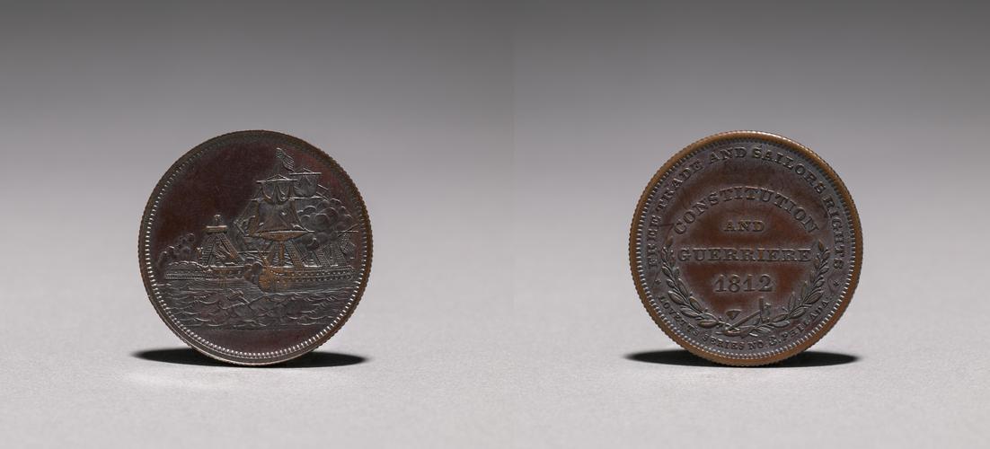
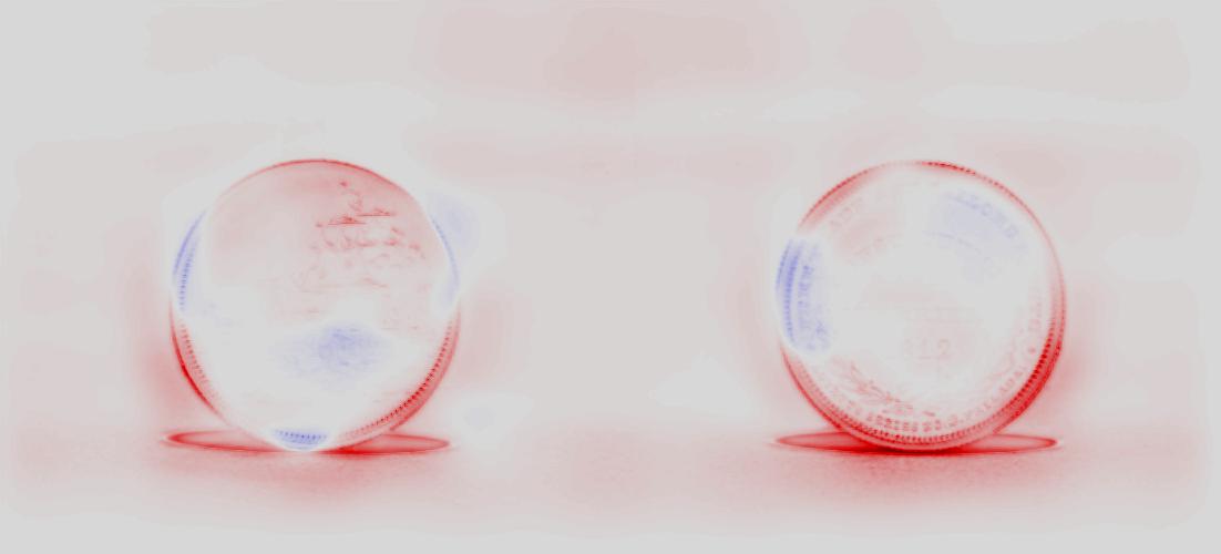
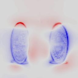
Figure 14: Example of coins within the Bronze class in HR&VS (left side) and LR&FS (right side), and its corresponding LRP explanations (bottom). Shape of coins is lost in LR&FS, which affects the prediction.
Cleveland museum: 1916.1877

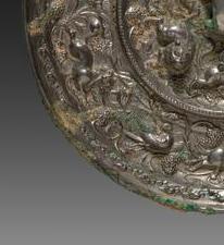
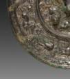
Figure 15: Zoom in of a Bronze artwork in HR&VS (left) and in LR&FS (right) respectively. Notice how the corrosion and patinas are easier to appreciate in HR&VS.
Cleveland museum: 1926.248

6 Conclusions

In this paper, we introduce the MAMe dataset, a novel challenge for the prediction of artwork mediums based on its visual appearance. The images of the dataset come from three different museums for a total of 37,407 images. Museums do not share a common scheme for labeling mediums, which required intensive work by art experts for its homogenization. For producing the dataset, we leverage technical requirements (sample size, balance, image resolution, etc.) and domain requirements (visual coherency, taxonomical properties, etc.). At the end, the MAMe is composed by 29 classes of mediums, each containing at least 850 images (always 700 for training) of high resolution (at least 500 pixels in the smaller axis) and variable shape.

In comparison with commonly available datasets, the MAMe provides a significantly larger distribution of high resolution and variable-shaped images. These properties are of relevance for future applications in domains such as medicine or autonomous driving; domains where attention to detail, understanding the overall structure and avoiding image pattern deformation/loss is crucial. Recognizing a lack of focus on these topics by the AI community, MAMe provides a good testing environment for new research ideas in the field.

Baselines and hypothesis results provide several conclusions. Regarding baselines, results presented in Table 4 show the capability of such models to solve the task proposed by the MAMe dataset up to certain degree, with a top performance of 88.95% accuracy achieved by EfficientNet-B3 architecture using R360k-FS data format. Regarding hypothesis evaluation, results shown in Table 4 and Figure 5 support H₁ and H₃ hypotheses but not H₂. We conclude from our first hypothesis H₁ that performance on the MAMe task increases when using images of high resolution over standard low resolution ones. Furthermore, based on the validated third hypothesis H₃, we see that this performance gain comes not only from larger image resolution but also from an increase of the image information (unlike ImageNet [1]). In contrast, results on the H₂ hypothesis do not validate it. We consider prototypical architectures to be specifically designed for FS data, hence not taking proper advantage of the VS property. Moreover, the current way of handling VS introduce padding on batching, increasing the amount of noise during training, specially in high resolution settings (i.e., R360k in our case). We consider that there is room for improvement in this area based on studies in a previous version of the MAMe dataset, where padding reduction on VS models provides performance improvements of 3% to 5% [44].

Lastly, we perform an explainability and expert analysis to further understand the differences when training models with either, low resolution and fixed-shape (R65k-FS) images or high resolution and variable-shape (A500-VS). The results of these analysis allow us to assess how the models we explored fail to discriminate between certain classes due to a lack of resolution. In several cases we found that even the A500-VS resolution is insufficient to perceive the patterns that experts would pay attention to. This forces the models to learn on alternative patterns that may not generalize well.

Overall, the MAMe dataset constitutes a large scale challenge which benefits from the use of HR. Benefit from using HR images does not only come from bigger internal representation of the models, but also from an increase of the image information. This is particularly characteristic for MAMe, since differs from the prototypical and well-known ImageNet dataset. Further research is needed to efficiently handle VS data, and MAMe dataset serves as a good candidate for such use case.

References

- Russakovsky et al. [2015] Olga Russakovsky, Jia Deng, Hao Su, Jonathan Krause, Sanjeev Satheesh, Sean Ma, Zhiheng Huang, Andrej Karpathy, Aditya Khosla, Michael Bernstein, et al. Imagenet large scale visual recognition challenge. International journal of computer vision, 115(3):211–252, 2015.
- Szegedy et al. [2015] Christian Szegedy, Wei Liu, Yangqing Jia, Pierre Sermanet, Scott Reed, Dragomir Anguelov, Dumitru Erhan, Vincent Vanhoucke, and Andrew Rabinovich. Going deeper with convolutions. In Proceedings of the IEEE conference on computer vision and pattern recognition, pages 1–9, 2015.
- He et al. [2016] Kaiming He, Xiangyu Zhang, Shaoqing Ren, and Jian Sun. Deep residual learning for image recognition. In Proceedings of the IEEE conference on computer vision and pattern recognition, pages 770–778, 2016.
- Srivastava et al. [2014] Nitish Srivastava, Geoffrey Hinton, Alex Krizhevsky, Ilya Sutskever, and Ruslan Salakhutdinov. Dropout: a simple way to prevent neural networks from overfitting. The journal of machine learning research, 15(1):1929–1958, 2014.
- Nair and Hinton [2010] Vinod Nair and Geoffrey E Hinton. Rectified linear units improve restricted boltzmann machines. In Proceedings of the 27th international conference on machine learning (ICML-10), pages 807–814, 2010.
- Glorot and Bengio [2010] Xavier Glorot and Yoshua Bengio. Understanding the difficulty of training deep feedforward neural networks. In Proceedings of the thirteenth international conference on artificial intelligence and statistics, pages 249–256, 2010.
- He et al. [2015] Kaiming He, Xiangyu Zhang, Shaoqing Ren, and Jian Sun. Delving deep into rectifiers: Surpassing human-level performance on imagenet classification. In Proceedings of the IEEE international conference on computer vision, pages 1026–1034, 2015.
- [8] Beyond imagenet large scale visual recognition challenge. http://image-net.org/challenges/beyond_ilsvrc. Accessed: 2019-11-14.
- Xie et al. [2019] Qizhe Xie, Eduard Hovy, Minh-Thang Luong, and Quoc V. Le. Self-training with noisy student improves imagenet classification, 2019.
- Simonyan and Zisserman [2014] Karen Simonyan and Andrew Zisserman. Very deep convolutional networks for large-scale image recognition. arXiv preprint arXiv:1409.1556, 2014.
- Szegedy et al. [2016] Christian Szegedy, Vincent Vanhoucke, Sergey Ioffe, Jon Shlens, and Zbigniew Wojna. Rethinking the inception architecture for computer vision. In Proceedings of the IEEE conference on computer vision and pattern recognition, pages 2818–2826, 2016.
- Zoph et al. [2018] Barret Zoph, Vijay Vasudevan, Jonathon Shlens, and Quoc V Le. Learning transferable architectures for scalable image recognition. In Proceedings of the IEEE conference on computer vision and pattern recognition, pages 8697–8710, 2018.
- Huang et al. [2019] Yanping Huang, Youlong Cheng, Ankur Bapna, Orhan Firat, Dehao Chen, Mia Chen, HyoukJoong Lee, Jiquan Ngiam, Quoc V Le, Yonghui Wu, et al. Gpipe: Efficient training of giant neural networks using pipeline parallelism. In Advances in Neural Information Processing Systems, pages 103–112, 2019.
- He et al. [2017] Kaiming He, Georgia Gkioxari, Piotr Dollár, and Ross Girshick. Mask r-cnn. In Proceedings of the IEEE international conference on computer vision, pages 2961–2969, 2017.
- Lin et al. [2017] Tsung-Yi Lin, Piotr Dollár, Ross Girshick, Kaiming He, Bharath Hariharan, and Serge Belongie. Feature pyramid networks for object detection. In Proceedings of the IEEE conference on computer vision and pattern recognition, pages 2117–2125, 2017.
- Tan and Le [2019] Mingxing Tan and Quoc V Le. Efficientnet: Rethinking model scaling for convolutional neural networks. arXiv preprint arXiv:1905.11946, 2019.
- Ghosh et al. [2019] Swarnendu Ghosh, Nibaran Das, and Mita Nasipuri. Reshaping inputs for convolutional neural network: Some common and uncommon methods. Pattern Recognition, 93:79–94, 2019.
- Geras et al. [2017] Krzysztof J Geras, Stacey Wolfson, Yiqiu Shen, Nan Wu, S Kim, Eric Kim, Laura Heacock, Ujas Parikh, Linda Moy, and Kyunghyun Cho. High-resolution breast cancer screening with multi-view deep convolutional neural networks. arXiv preprint arXiv:1703.07047, 2017.
- Lotter et al. [2017] William Lotter, Greg Sorensen, and David Cox. A multi-scale cnn and curriculum learning strategy for mammogram classification. In Deep Learning in Medical Image Analysis and Multimodal Learning for Clinical Decision Support, pages 169–177. Springer, 2017.
- Chen et al. [2017] Xiaozhi Chen, Huimin Ma, Ji Wan, Bo Li, and Tian Xia. Multi-view 3d object detection network for autonomous driving. In Proceedings of the IEEE Conference on Computer Vision and Pattern Recognition, pages 1907–1915, 2017.
- Treml et al. [2016] Michael Treml, José Arjona-Medina, Thomas Unterthiner, Rupesh Durgesh, Felix Friedmann, Peter Schuberth, Andreas Mayr, Martin Heusel, Markus Hofmarcher, Michael Widrich, et al. Speeding up semantic segmentation for autonomous driving. In MLITS, NIPS Workshop, volume 2, page 7, 2016.
- Kuznetsova et al. [2018] Alina Kuznetsova, Hassan Rom, Neil Alldrin, Jasper Uijlings, Ivan Krasin, Jordi Pont-Tuset, Shahab Kamali, Stefan Popov, Matteo Malloci, Tom Duerig, and Vittorio Ferrari. The open images dataset v4: Unified image classification, object detection, and visual relationship detection at scale. arXiv:1811.00982, 2018.
- Huang et al. [2017] Gao Huang, Zhuang Liu, Laurens Van Der Maaten, and Kilian Q Weinberger. Densely connected convolutional networks. In Proceedings of the IEEE conference on computer vision and pattern recognition, pages 4700–4708, 2017.
- Sandler et al. [2019] Mark Sandler, Jonathan Baccash, Andrey Zhmoginov, and Andrew Howard. Non-discriminative data or weak model? on the relative importance of data and model resolution, 2019.
- Bossard et al. [2014] Lukas Bossard, Matthieu Guillaumin, and Luc Van Gool. Food-101–mining discriminative components with random forests. In European Conference on Computer Vision, pages 446–461. Springer, 2014.
- Wu et al. [2019] Xiaoping Wu, Chi Zhan, Yu-Kun Lai, Ming-Ming Cheng, and Jufeng Yang. Ip102: A large-scale benchmark dataset for insect pest recognition. In Proceedings of the IEEE Conference on Computer Vision and Pattern Recognition, pages 8787–8796, 2019.
- Zhou et al. [2017] Bolei Zhou, Agata Lapedriza, Aditya Khosla, Aude Oliva, and Antonio Torralba. Places: A 10 million image database for scene recognition. IEEE transactions on pattern analysis and machine intelligence, 40(6):1452–1464, 2017.
- Quattoni and Torralba [2009] Ariadna Quattoni and Antonio Torralba. Recognizing indoor scenes. In Computer Vision and Pattern Recognition, 2009. CVPR 2009. IEEE Conference on, pages 413–420. IEEE, 2009.
- Nilsback and Zisserman [2008] Maria-Elena Nilsback and Andrew Zisserman. Automated flower classification over a large number of classes. In Computer Vision, Graphics & Image Processing, 2008. ICVGIP’08. Sixth Indian Conference on, pages 722–729. IEEE, 2008.
- Parkhi et al. [2012] Omkar M Parkhi, Andrea Vedaldi, Andrew Zisserman, and CV Jawahar. Cats and dogs. In Computer Vision and Pattern Recognition (CVPR), 2012 IEEE Conference on, pages 3498–3505. IEEE, 2012.
- Khosla et al. [2011] Aditya Khosla, Nityananda Jayadevaprakash, Bangpeng Yao, and Fei-Fei Li. Novel dataset for fine-grained image categorization: Stanford dogs. In Proc. CVPR Workshop on Fine-Grained Visual Categorization (FGVC), volume 2, 2011.
- Cimpoi et al. [2014] Mircea Cimpoi, Subhransu Maji, Iasonas Kokkinos, Sammy Mohamed, and Andrea Vedaldi. Describing textures in the wild. In Proceedings of the IEEE Conference on Computer Vision and Pattern Recognition, pages 3606–3613, 2014.
- Griffin et al. [2007] Gregory Griffin, Alex Holub, and Pietro Perona. Caltech-256 object category dataset. 2007.
- Lin et al. [2014] Tsung-Yi Lin, Michael Maire, Serge Belongie, James Hays, Pietro Perona, Deva Ramanan, Piotr Dollár, and C Lawrence Zitnick. Microsoft coco: Common objects in context. In European conference on computer vision, pages 740–755. Springer, 2014.
- [35] M. Everingham, L. Van Gool, C. K. I. Williams, J. Winn, and A. Zisserman. The PASCAL Visual Object Classes Challenge 2012 (VOC2012) Results. http://www.pascal-network.org/challenges/VOC/voc2012/workshop/index.html.
- Foundation [2019] Common Visual Data Foundation. Google landmarks v2 dataset. https://github.com/cvdfoundation/google-landmark##release-history, 2019.
- Maynor and Reyden [1993] Catherine I Maynor and D Reyden. Paper conservation catalog. The American Institute for Conservation of Historic and Artistic Works Book and Paper Group. Ninth Edition., 1993.
- Met [a] Met museum: Image and data resources. https://www.metmuseum.org/about-the-met/policies-and-documents/image-resources, a. Accessed: April 2020.
- [39] Lacma launches new collections online website. https://www.lacma.org/press/lacma-launches-new-collections-online-website. Accessed: April 2020.
- [40] Cleveland museum: Open access. https://www.clevelandart.org/open-access. Accessed: April 2020.
- Met [b] Printmaking descriptions. https://www.metmuseum.org/about-the-met/curatorial-departments/drawings-and-prints/materials-and-techniques/printmaking, b. Accessed: May 2020.
- Reddi et al. [2019] Sashank J Reddi, Satyen Kale, and Sanjiv Kumar. On the convergence of adam and beyond. arXiv preprint arXiv:1904.09237, 2019.
- Kingma and Ba [2014] Diederik P Kingma and Jimmy Ba. Adam: A method for stochastic optimization. arXiv preprint arXiv:1412.6980, 2014.
- Sotiropoulos [2020] Ioannis Nektarios Sotiropoulos. Handling variable shaped & high resolution images for multi-class classification problem. Master’s thesis, Universitat Politècnica de Catalunya, 2020.
- Lipton [2018] Z.C. Lipton. The mythos of model interpretability: In machine learning, the concept of interpretability is both important and slippery. Queue, 16, 05 2018.
- Selvaraju et al. [2019] Ramprasaath R. Selvaraju, Michael Cogswell, Abhishek Das, Ramakrishna Vedantam, Devi Parikh, and Dhruv Batra. Grad-cam: Visual explanations from deep networks via gradient-based localization. International Journal of Computer Vision, 128(2):336–359, Oct 2019. ISSN 1573-1405. doi:10.1007/s11263-019-01228-7. URL http://dx.doi.org/10.1007/s11263-019-01228-7.
- Simonyan et al. [2013] Karen Simonyan, Andrea Vedaldi, and Andrew Zisserman. Deep inside convolutional networks: Visualising image classification models and saliency maps, 2013.
- Springenberg et al. [2014] Jost Tobias Springenberg, Alexey Dosovitskiy, Thomas Brox, and Martin Riedmiller. Striving for simplicity: The all convolutional net, 2014.
- Sundararajan et al. [2017] Mukund Sundararajan, Ankur Taly, and Qiqi Yan. Axiomatic attribution for deep networks, 2017.
- Zeiler and Fergus [2013] Matthew D Zeiler and Rob Fergus. Visualizing and understanding convolutional networks, 2013.
- Lapuschkin et al. [2015] Sebastian Lapuschkin, Alexander Binder, Grégoire Montavon, Frederick Klauschen, Klaus-Robert Müller, and Wojciech Samek. On pixel-wise explanations for non-linear classifier decisions by layer-wise relevance propagation. PLoS ONE, 10:e0130140, 07 2015. doi:10.1371/journal.pone.0130140.
- Arbabzadah et al. [2016] Farhad Arbabzadah, Grégoire Montavon, Klaus-Robert Müller, and Wojciech Samek. Identifying individual facial expressions by deconstructing a neural network. In Bodo Rosenhahn and Bjoern Andres, editors, Pattern Recognition, pages 344–354, Cham, 2016. Springer International Publishing. ISBN 978-3-319-45886-1.
- Sturm et al. [2016] Irene Sturm, Sebastian Bach, Wojciech Samek, and Klaus-Robert Müller. Interpretable deep neural networks for single-trial EEG classification. CoRR, abs/1604.08201, 2016. URL http://arxiv.org/abs/1604.08201.
- Thomas et al. [2018] Armin W Thomas, Hauke R Heekeren, Klaus-Robert Müller, and Wojciech Samek. Interpretable lstms for whole-brain neuroimaging analyses. Preprint at https://arxiv. org/abs/1810.09945, 2018.
- Binder et al. [2018] Alexander Binder, Michael Bockmayr, Miriam Hägele, Stephan Wienert, Daniel Heim, Katharina Hellweg, Albrecht Stenzinger, Laura Parlow, Jan Budczies, Benjamin Goeppert, Denise Treue, Manato Kotani, Masaru Ishii, Manfred Dietel, Andreas Hocke, Carsten Denkert, Klaus-Robert Müller, and Frederick Klauschen. Towards computational fluorescence microscopy: Machine learning-based integrated prediction of morphological and molecular tumor profiles, 2018.
- Montavon et al. [2019] Grégoire Montavon, Alexander Binder, Sebastian Lapuschkin, Wojciech Samek, and Klaus-Robert Müller. Layer-Wise Relevance Propagation: An Overview, pages 193–209. 09 2019. ISBN 978-3-030-28953-9. doi:10.1007/978-3-030-28954-6_10.