Adaptive Height Optimisation for Cellular-Connected UAVs: A Deep Reinforcement Learning Approach

Abstract

Providing reliable connectivity to cellular-connected Unmanned Aerial Vehicles can be very challenging; their performance highly depends on the nature of the surrounding environment, such as density and heights of the ground Base Stations. On the other hand, tall buildings might block undesired interference signals from ground BSs, thereby improving the connectivity between the UAVs and their serving BSs. To address the connectivity of UAVs in such environments, this paper proposes a Reinforcement Learning (RL) algorithm to dynamically optimise the height of a UAV as it moves through the environment, with the goal of increasing the throughput or spectrum efficiency that it experiences. The proposed solution is evaluated in two settings: using a series of generated environments where we vary the number of BS and building densities, and in a scenario using real-world data obtained from an experiment in Dublin, Ireland. Results show that our proposed RL-based solution improves UAV Quality of Service (QoS) by 6% to 41%, depending on the scenario. We also conclude that, when flying at heights higher than the buildings, building density variation has no impact on UAV QoS. On the other hand, BS density can negatively impact UAV QoS, with higher numbers of BSs generating more interference and deteriorating UAV performance.

I Introduction

UAVs can leverage 5G connectivity to perform different applications, such as security surveillance, search and rescue operations, and building inspections. However, providing reliable connectivity to such UAVs is still an open problem, as they present a paradigm shift when compared to their ground counterparts such as smartphones. According to the specifications (release 14 of 3rd Generation Partnership Project (3GPP) [release14]), a UAV needs to maintain continuous connectivity with the mobile network at speeds up to 300km/h.

Previous work, such as [rami1, rami2], investigates the feasibility of using existing network infrastructure to provide reliable wireless connectivity for UAVs. These studies conclude that currently deployed networks would need to adapt some of their design configurations, such as increasing BS heights [reshape] or changing the tilt of the antennas [network-adapt] so as to enable connectivity for UAVs. Redesigning the terrestrial network infrastructure may be unfeasible, and an adaptable solution on the UAV side may be necessary to accelerate the UAV integration into the network.

Due to the height at which UAVs fly, there are often no obstacles and therefore no blockage between the UAVs and their serving BS. However, at high altitudes, the increased probability of Line-of-Sight (LoS) to ground BSs results in high levels of interference at the UAVs. The work in [reshape] states that the optimal height at which the UAV can fly to maintain reliable communication depends on the BS density and height. Similarly, the authors in [rami3] show that the vertical movements of the UAV affect their coverage probability.

Motivated by the above, this paper proposes a RL approach for dynamic optimisation of the height of a UAV connected to the cellular network once it moves through a city. We propose optimising the altitude of the UAV, separating it from the problem of a horizontal trajectory decision. We separate it from the horizontal optimisation trajectory as in some applications, such as surveillance and organ delivery, the horizontal path will be defined by the application, and only the altitude will have the freedom to be adapted. We evaluate our proposed approach with generated environment and a experimental measurement dataset. We investigate the proposed solution in a generated environment to evaluate which are the main characteristics to influence the approach. In this environment, we vary the BS and building densities to understand if these variables interfere with the optimal UAV altitude.

Then to complement the investigation we adapt the proposed approach to be used with data collected from real-world scenario. To the best of our knowledge, this is the first work to optimise connectivity of a cellular-connected UAV by dynamically adapting the height at which it is flying, as well as the first to evaluate a UAV connectivity optimisation approach on experimentally-obtained real-world data. The main contributions of this paper are described bellow:

• We define a problem of optimising QoS of an UAV as an RL problem, defining states and actions.

• We propose a solution to adapt the UAV’s height dynamically, which uses Deep Q-Learning (DQN) and replay memory to optimise QoS parameters as the spectrum efficiency and throughput.

• We provide an evaluation of the influence of building density on the UAV height adaptation.

• We provide an evaluation of the proposed solution in a generated environment and using a real-world based dataset.

• We analyse how the proposed solution and the baselines affect the height.

The remainder of the paper is organised as follows. In Section II we discuss the existing work done on the issue of connectivity of UAVs to the wireless network. In Section III we present the system model of our generated environment. In Section IV we introduce the problem statement, where we define the scenario and how the UAV moves. In Section V the design and implementation of our proposed RL solution is explained. We detail the parameters of our RL model, as well as the algorithm. In Section VI, we evaluate our solution for the scenario where we use generated data. In Section VII-A we introduce the real-world dataset and detail small changes on the proposed solution to use this data, then in Section VII, we present the results using the real-world dataset. Finally, in Section LABEL:sec:conclusion, we conclude the paper and discuss the issues that remain open for future work.

II UAV movement optimisation: Related Work

The works on trajectory optimisation focus on 2D optimisation and rarely mention the height or the UAV. In this section, we introduce works that optimise the trajectory considering the UAV-BS access link.

[HTML]C0C0C0                                    [HTML]C0C0C0Paper				[HTML]C0C0C0Type of UAV	[HTML]C0C0C0Optimise	[HTML]C0C0C0Method
[trajectory1]	Connected UAV	Distance to BS	Graph
[rami3]	connected UAV	Coverage Prediction	Cauchy’s inequality
[trajec-mobile]	Connected UAV	Horizontal Optimisation	Graph
[rival]	Connected UAV	Horizontal Optimisation	Deep RL
[3d-2]	UAV BS	3D position	Bisection search
[3d-1]	UAV BS	3D position	Particle swarm optimisation
[3d-3]	UAV BS	3D position	DQN

TABLE I: UAV movement optimisation works.

In [trajec-mobile], the authors propose optimising the horizontal path of a cellular connected UAV that flies from an initial to a final location, while maintaining reliable communication with the underlying mobile network. This approach proposes that the UAV flies at the fixed minimum height allowed by the regulatory entities. In this study, the authors do not consider the interference from BSs to which the UAV is not connected and blockage from the buildings blocking the link from UAV to BS. To accomplish the study objectives, a graph representation of the network is proposed, with 3 solutions: first, a graph where each node is a BS; second, a graph where the nodes are the handover points between the BSs; and third, where the handover points are the optimal point in an intersection area. Dijkstra algorithm is used to find the route of the UAV and show it is close to the optimal solution. Height optimisation was not considered, and the authors conclude that introducing a height variable to the problem is not a trivial task and that their proposed horizontal trajectory solution is not the most appropriate one for 3D movement. They conclude that it would be unfeasible to represent all the possible heights a UAV could have at all the nodes, as each of them should be a new node increasing the system’s complexity.

The work in [rival] creates an optimised path with the objective of maintaining a uninterrupted connection to the BSs. This work only considers the uplink from the UAV to the BS network. This work also highlights the importance of the altitude of the UAV and calculates the upper and lower bounds for the height at which the UAV should fly to satisfy the minimum rate requirements of the uplink, considering the known BSs locations. Authors calculate a range of heights at which the UAV should fly to provide a minimum achievable rate. In addition, building blockage on the link UAV - BS is not considered. With this approach, each UAV decides its next horizontal location. The authors conclude that the altitude is vital to minimise the transmission delay of the UAV and that it should be a function of the ground network density, network parameters as the transmission power, ground network data requirements and the UAV’s action. The exact height of the UAV is not calculated as it would increase the complexity of the algorithm exponentially.

The height planning of a connected UAV is a new field, however several works have studied the height placement of UAVs acting as BSs. The techniques used to optimise the heights at which a UAV acting as a BS should fly can also overlap with our problem of interest as it also consider the radio link between a UAV and a element that is located at lower heights.

In many examples of the prior art, works on UAV wireless connectivity, either for UAV as network end-user or UAV as BS, did not consider the effect of interference conditions. The quality of the link between UAV and a BS can suffer from interference coming from other BSs, from objects or buildings intercepting the directional connection between them (shadow zone), or even the natural fading on the propagation. The work in [44] assumes UAV as BS and provides coverage to Ground User Equipments. The authors propose a sigmoid model to investigate the probability of LoS channel in the UAV - GUE link as a function of the vertical angle between them. In the paper, a UAV with an omnidirectional antenna flies over an urban area. The authors do not consider any source of interference, leaving the link limited with only the path loss. They conclude that a bigger angle decreases the probability of a building block the link. They also add that there exists an optimal height for the UAV BS, which increases the coverage area.

In [61] and [62], authors applied stochastic geometry to model the coverage probability of a UAV-BS network in a fading-free and Nakagami-m fading channel. The authors fix the number of UAVs operating in an area at a certain height above the ground and demonstrate that with an increase in height, the coverage probability decreases. Also, in [62] authors demonstrate that bigger values of fading parameter reduce the variance of the Signal-to-Interference-and-Noise Ratio (SINR) for the GUE.

In [3d-2] authors propose the approach to calculate the 3D position of UAV as a BS, by applying the interior point optimiser of bisection search. Their main objective is to maximise the coverage area by a UAV cell without providing to a GUE a QoS below a threshold. They consider building blockage and non-Line-of-Sight (NLoS) between the UAV as BS and its users. The covered area changes depending on UAV’s height, and for the lower density of GUEs the coverage is larger when compared to higher density, showing the worst coverage for urban scenarios.

In [3d-1], the authors find the optimal positions for a network of UAV as BS in order to minimise the number of BSs required to provide the needed QoS for their users. The study considers the blockage generated by buildings in an urban area and NLoS occurrences between the UAV and its users. The proposed solution used an heuristic algorithm based on the number of BS that can serve the GUE, coverage and capacity requirements. The number of users on the network was essential to define the height and number of UAVs as BSs. The authors concluded that with their solution it is possible to decrease the amount of UAV as BS and provide the same quality on data rate.

Similarly, the work in [3d-3] proposes a 3-step solution for horizontal and vertical optimisation for UAV-BSs with different machine learning algorithms for each step. The bounds of the UAV height are the UAV maximum transmission power for its greatest height, and the minimum required distance between the UAV and the users, defined by the regulatory entities, for the minimum height. In the first instance, it considers a static problem, where the users of the network do not move. As a first step, it partitions the area into cells for the UAV-BSs to cover, by applying K-means (GAK-means) algorithm. Next, it uses a Q-learning algorithm, where each UAV is an agent and has to decide its position by learning from its mistakes. As the final step, they consider a scenario where users move between BSs and the network have to adapt to these movements. The authors apply Deep Neural Network (DNN), as it enables each UAV to gradually learn the dynamic movements of the users. They conclude that the proposed solution outperforms the K-means algorithm and IGK algorithm with low complexity.

The UAV-BS scenario defers from the connected UAV problem because the connect UAV moves through the city and do not divide it into cells, so the use of K-mean for clustering, for example, is not applicable. However, the use of RL to adapt its height depending on the cellular network radio technology and the regulatory entities definitions is a valuable insight. To apply DNN into the connected UAV scenario, one needs to investigate what is relevant to a UAV as User Equipment (UE), which are the information a UE has from its connection, how the UAV can interact with the environment, and design a model that can learn all these characteristics and be effective through different topologies.

Table II provides a summary of the state of the art in connected UAV movement optimisation.

While some existing work has looked into optimising the height of UAV BSs, there is a significant lack of work looking at UAVs when they are the end users. In this paper, we propose dynamically optimising the altitude of the UAV. The proposed solution applies RL to decide, based on environmental measurements, if the UAV needs to move above, below, or stay at the same height in order to experience the best QoS possible from the cellular network in the long run.

III System Model

We consider an urban scenario where a UAV flies while connected to the cellular network. The UAV’s initial and final positions are denoted as $(x_{1},y_{1},z_{1})$ and $(x_{f},y_{f},z_{f})$, with $f$ representing the total number of discrete steps in the experiment. $x$ and $y$ denote coordinates on the horizontal plane, while $z$ denotes height above ground. At each step, the UAV moves in the $x$ coordinate in direction to its final destination.

III-1 Building and BS distribution

The buildings distributed in the area might affect the UAV LoS, as they can block the channel between the UAV and the BSs. In order to check if a signal is in LoS or not, we verify if there is a tall enough building between the UAV and BS. If the signal is blocked by a building, NLoS, it causes the signal to be attenuated, which is reflected in the SINR expression in Equation 1. We use a commonly-adopted model for the urban environment which models the buildings as a square grid with the locations of building centerpoints $(x_{bl},y_{bl})$, that was presented in [ITUR_2012] and used in works as [galkincoverage, 3d-1, 3d-2]. The area occupied by each building, $Bl_{a}$, is constant, and the density of buildings, $Build_{dens}$, is denominated by the number of building per square kilometre. The individual building height, $h_{b}l$ is randomly distributed according to a Poisson distribution, with scale parameter $a$.

To define the position of the building centerpoints and BSs we run a Poisson distribution with the building and BS densities as input.

III-2 UAV and BS Antennas

The UAV is equipped with one omnidirectional antenna to connect to a serving BS and receive data. The antenna has an omnidirectional radiation pattern, and it has an antenna gain equal to 1. We express the coordinates of the BS which the UAV is associated as $b_{s}=\{x_{s},y_{s}\}\in\Phi$ and its horizontal distance to the UAV as $r_{s}$. The BSs that the UAV is not connected will be called as neighbours BSs.

The BS has a directional antenna with a horizontal and vertical beam-width $\omega$ along with a rectangular radiation pattern; The antenna gain is defined as $\eta(\omega)=0$ outside of the main lobe; and $16\pi/(\omega^{2})$ inside of the main lobe.

Spectrum efficiency $SE$ is the maximum bit rate that can be transmitted per unit of bandwidth. It is a measure of the QoS in the network. The Shannon–Hartley theorem bounds the maximum achievable rate a user can reach once it establishes a wireless link. As we want to improve user’s experience providing reliable connectivity to UAVs, our purpose is to increase spectrum efficiency. We calculate the spectrum efficiency value for the calculated SINR based on Shannon–Hartley theorem. The SINR is a function of the antenna gain and channel model and given as:

$$SINR=\frac{p\eta(\omega)c(\Delta x^{2}+\Delta y^{2})^{-\alpha_{t_{s}}/2}}{I_{L}+I_{N}+\sigma^{2}}$$ (1)

where $p$ is the BS transmit power, $\alpha_{t_{s}}$ is the pathloss exponent, $t_{s}\in\{\text{L},\text{N}\}$ indicates whether the UAV has LoS or NLoS to its serving BS, $\Delta x^{2}$ and $\Delta y^{2}$ is the distance between the BS and the UAV, $c$ is the near-field pathloss, $\sigma^{2}$ is the noise power, and $I_{L}$ and $I_{N}$ are the aggregate interference from LoS and NLoS, respectively.

III-3 Horizontal route adaptation

The UAV horizontal route is defined by an independent approach that focuses on bringing the UAV closer to the BS it is connected. We introduce this adaptation to the horizontal path so we can investigate the independence of the proposed height adaptation method to the horizontal route. The UAV flies in direction to its final destination but approximates its Y trajectory to get closer to the BS that it is connected by $d$. At every time step, the UAV connects to the BS with stronger SINR and get closer in the Y coordinates to this BS by $d$, being maximum of $d$ distant to the straight line between $(x_{1},y_{1})$ and $(x_{f},y_{f})$ as illustrated in Figure 1(b). The focus of our approach is to investigate if the approach is able to adapt the height of the UAV and can adapt to any underlying routes decision that a UAV might take during its path, showing its independence from the horizontal path decisions.

III-4 UAV-BS Link

The UAV connects to the BS with the best SINR at all times. Therefore, as the UAV moves through the environment some BSs become stronger and others weaker. When it reaches the point where its serving BS is no longer the BS with strongest signal, it will reconnect to the new LoS with the strongest signal. We assume that this handover occurs seamlessly, and there is no disconnect or loss of signal quality when it happens.

We assume that the UAV will have access to the SINR measurements from the BS it is connected to and from the 5 neighbours BS with strongest signals, the spectrum efficiency it is achieving with the serving BSs, and its height at all steps. SINR and spectrum efficiency data is easily obtained by the UAV from its cellular connection, while the height information is obtained via other UAV sensors located on the UAV.

IV Problem Statement

In this work, as the focus is on UAV height optimisation and many approaches for optimising 2D trajectories already exist, we assume a simple horizontal path. Note that simplification of the path does not affect the applicability of our proposed approach, as due to its design, it can be integrated with more complex horizontal path algorithms (which are out of the scope of this paper). In other words, the only coordinate that can be optimised is $z$. We assume that the maximum height change at each time step is $d$, so $|z_{t}-z_{t-1}|\leq d$, where $|.|$ denotes absolute value.

Usually, UAVs are allowed to fly in a height range defined by safety regulation, with the minimum allowed height denoted as $Z_{min}$, and the maximum allowed height as $Z_{max}$. We assume that the UAV starts at $Z_{min}$. Figure 1 shows UAVs horizontal movement and vertical movement in the generated environment analyses. Figure 1(a) illustrates the possible path of the UAV, where $d$ is the maximum distance the UAV can move up or down in each step. It is an representation of a limitation of how much a UAV can move realistic up or down and horizontally in a time-step.

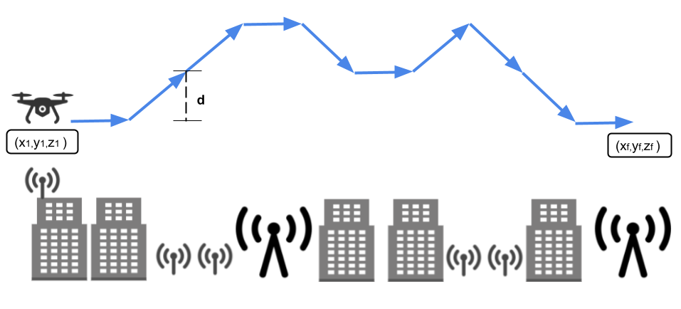
(a) Side view of a UAV connected to the mobile network adjusting its height to maximise its spectrum efficiency.

(b) Top view of a UAV connected to the mobile network when it moves closer to the connected BS through the path in an urban area from position ($x_{1},y_{1}$) to the final position ($(x_{f},y_{f})$). In red shows which BS the UAV is connected at each point of the trajectory.

Figure 1: UAV vertical and horizontal movement assumed in this paper.

Our main objective is to optimise $z$ coordinate at each step, in order to improve the QoS experienced by the UAV. The metric used to represent the QoS is the spectrum efficiency $SE$.

We formulate the optimisation problem as follows:

$$\underset{(z_{1},...,z_{f-1},z_{f})}{\text{max}}\quad\sum_{t=1}^{f}SE(t);$$ (2a)

s.t. $$z_{t}>Z_{min}\quad\forall\quad t$$ (2b)

$$z_{t}<Z_{max}\quad\forall\quad t$$ (2c)

$$|z_{t}-z_{t-1}|\leq d\quad\forall\quad t$$ (2d)

We assume that the UAV will have access to the SINR measurements from its connection, the spectrum efficiency $SE$ of its actual location, and its height at all steps. SINR and spectrum efficiency data is easily obtained by the UAV from its cellular connection, while the height information is obtained via other UAV sensors located on the UAV.

V Proposed Solution

Figure 2: Graphical representation of the designed DNN.

To solve the height optimisation problem for a specific position of the UAV given a particular topology of the BSs and buildings, one could apply stochastic geometry as in [boris_dic_ant]. The main issue with this approach is that to represent this problem via stochastic geometry, one has to know the statistical distribution of the features of the environment for each position that the UAV assumes during flight. This can be computationally expensive to run and the environmental statistics may not be accurate to what the UAV would find once it is flying in the real world.

V-A RL agent definition

To tackle this issue our solution is based on RL. In particular, we apply DQN as it does not require a predefined model of the environment, since it learns by interacting with the environment in an online manner. The agent of our model is the UAV, as it is the one taking the action of changing the height. Bellow we define the other main components of our model.

State Space $S$

$S$ is all the possible values of the state, and $s$ is the individual single value of the state. We just considered in the state space values a normal UE would have from the network and measurements of sensors that a UAV should have to have a safe fly. Follow the components of $S$:

• Height $z$: which is obtained by UAV sensors and it is relevant for UAV’s decision-making process, as in order to know whether to move next and stay within the hard limits.

• Received $SINR$ and the strongest 5 SINR of neighbours BSs-$SINRn$: which is obtained by UE sensors to perform the measurement reports. This value impacts the UE QoS that is what we intent to maximise.

• 4 last $z$, $SINR$, $SINRn$, $a$, $r$: which will be stored from the previous steps. In order to achieve better optimisation, we extended the state with the four previous $z$, $SINR$, action $a$ and reward $r$, following the lines of the original DQN implementation [sutton2018reinforcement], as well its implementation in UAV connectivity [reqiba].

The agent has as input at each time step $s_{t}$, where t represents the time step the follow state. $s=\{SINR_{t},z_{t},SINR_{t-1},z_{t-1},a_{t-1},r_{t-1},SINRn_{t-1}$ SINRt-2,zt-2,at-2,rt-2,SINRnt-2,SINRt-3,zt-3, at-3,rt-3,SINRnt-3,SINRt-4,zt-4,at-4,rt-4, SINRnt-4}.

Action Space $A$

The action is the adjustment of the UAV height. An action $a\in\{-d,0,+d\}$ will be taken at the end of each time-step, where:

• $a=-d\Rightarrow z_{t+1}=z_{t}-d$

• $a=0\Rightarrow z_{t+1}=z_{t}$

• $a=d\Rightarrow z_{t+1}=z_{t}+d$.

Reward $R$

As the primary goal of our approach is to improve the UAV QoS during flight, our reward at each time step $r_{t}$ is defined as the spectrum efficiency achieved after the action at point $x_{t+1}$ at height $z_{t+1}$ in the experiment.

Our model has three hidden layers, with 200 neurons in each. Figure 2 illustrates the graphical representation of the proposed DNN.

In our solution, we use epsilon greedy approach, this is an strategy to balance exploration and exploitation in RL algorithms. We selected the initial $\epsilon=1$, where we select an action at random, and we decrease it at every step of the training process until it reaches 0.05, which in our experiment took 30 steps to reach.

V-B Hyper-parameters

We needed to perform a deep investigation to choose the hyper-parameters and design the model. We changed several of the hyper-parameters and inputs of the model until finding the proposed one. These parameters were experimentally selected among a number of model variations in which the number of layers, number of neurons per layer, activation function, number of epochs, regularisation, and the inputs were varied. As we apply experience replay, the epochs are how many times the model is trained with the mini-batch at each time-step. Depending on the complexity of the DQN network (for example number of input features, number and size of layers), the training can be performed in a few steps, or require thousands or larger number of steps. However, for the UAV height adaptation scenario it is imperative to have as few training steps as possible, so that the model can learn to optimise height quickly in any new city environment is applied in. In order to have a fast adaptation in a new environment, the model needs to adapt its weights quickly to not interfere with the UAV performance at the end of the path. For this evaluation, the value of $\epsilon$ and $\epsilon$-decay are 1 and 0.9 respectively, effectively meaning that the proposed model trains in 30 steps. We apply replay memory as an strategy to accelerate the learning process, where at each step the model trains with the mini batch for the number of epochs.

V-C RL algorithm for UAV height optimisation

The pseudo-code of the RL algorithm to optimise $z_{t}$ is shown in Algorithm V-C. Some parameters must be chosen and passed as input to the code to run the algorithm. They are the $Z_{min}$ and $Z_{max}$, the minimum and maximum allowed height that the UAV could fly. $X$ and $Y$ are the vectors with the horizontal coordinates the UAV should acquire during its movement. Where $X={x_{1},x_{2},..,x_{f}}$ and $Y={y_{1},y_{2},..,y_{f}}$, as the horizontal path is predefined. $\epsilon$, $\epsilon_{Decay}$ and $\epsilon_{min}$ are needed to apply the $\epsilon$-greedy approach. The input $\epsilon$ is the starting value for $\epsilon$, and $\epsilon_{Decay}$ is a value that will multiply $\epsilon$ and reduce its value at each interaction until $\epsilon_{min}$.

$\beta$ and $\beta_{min}$ are, respectively, the batch array and the minimum size of the batch needed to apply memory replay. While using memory replay, the number of $epochs$ to train the model and the $Discount$ factor to calculate the new Q value ($newQ$) is required. Finally, $var$ is an integer that indicates how often the target model should be updated. The expected output of this algorithm is the UAV next height in the next step.

The first step of the proposed RL-based algorithm for UAV height optimisation is to initiate the DQN model and the target DQN model, lines 1 and 2, respectively. Then we initialise the UAV coordinates in line 3 and initialise variable $t$, which refers to the timestep the UAV is during the each step. The while statement in line 5 is the overall while loop that represents the full flight path of the UAV, and has as many steps as that set of $X$ and $Y$.

Inside the step loop, it is needed to update $t$ and collect the current value of $SINR$ and $SINRns$. Then, we update the state value in $s_{t}$. After that, we randomly select a number, $randomNum$, and compare its value to $\epsilon$ in line 10. This step is necessary to evaluate the comparison of the $\epsilon$-greedy approach. In line 10, we also check $t$ value to be at least 4, as we need the state information values from the last 4 states for the input of the model. If the condition is satisfied, which means $randomNum>\epsilon$ and $t>4$, we use the DQN model to predict the best action $a_{t}$. If the condition is not satisfied, we randomly choose the action $a_{t}$. Once the action $a_{t}$ is defined, we execute it in line 16, ie modify the UAV height, moving the UAV up or down if it does not go above the permitted flight boundaries ($Z_{min}$ and $Z_{max}$). Then, the UAV also moves based on the sets $X$ and $Y$ its horizontal coordinates to the next position in line 17. We obtain the reward which represents the quality of our selected action, and is later used to update the learning process. The reward $r_{t}$ is equal to the measure throughout after executing the action, as shown in line 18. The $\epsilon$ decrease value is then performed in lines 19 to 21. The $\epsilon$ decrease is needed to decrease the amount of of random actions we perform once the model is being trained.

Algorithm 1 RL-based algorithm for UAV height optimisation

$\epsilon$; $\epsilon_{Decay}$;$\epsilon_{min}$; {//$\epsilon$-greedy parameters} $d$; $Z_{min}$; $Z_{max}$;$x$;$y$;{//Coordinates parameters} $epochs$;$var$;$Discount$;{//Replay memory parameters}

1:  $DQNModel\leftarrow InitialiseDQLModel()$

2:  $targetDQNModel\leftarrow InitialiseDQLModel()$

3:  $(x_{t},y_{t},z_{t})\leftarrow(x_{1},y_{1},Z_{min})$

4:  $t\leftarrow 0$

5:  while  $(x_{t},y_{t})\neq(x_{f},y_{f})$ do

6:     $t\leftarrow t+1$

7:     $SINR_{t}\leftarrow uav.GetCurrentSINR(x_{t},y_{t},z_{t})$

8:     $SINRns_{t}\leftarrow Get.SINR.Neighbours(x_{t},y_{t},z_{t})$

9:     $s_{t}\leftarrow SINR_{t},SINRns_{t},z_{t},s_{t}$

10:     $\textit{randomNum}\leftarrow RandomNumber(0-1)$

11:     if $\textit{randomNum}>\epsilon$ and $t>4$  then

12:        $a_{t}\leftarrow\textit{DQNModel.predictMaxValue}(s_{t})$

13:     else

14:        $a_{t}\leftarrow\textit{Random}(+d,0,-d)$

15:     end if

16:     uav.takeSelectedHeightAction(d,a, $Z_{min}$, $Z_{max}$)

17:     $(x_{t},y_{t})\leftarrow(x_{t+1},y_{t+1})$

18:     $r_{t}\leftarrow uav.GetQoS(x_{t},y_{t},z_{t})$

19:     if $\epsilon$ ¿ $\epsilon_{min}$ then

20:        $\epsilon\leftarrow\epsilon*\epsilon_{Decay}$

21:     end if

22:     $s_{t+1}\leftarrow a_{t},r_{t},s_{t}.removeState(s_{-4t})$

23:     $\beta\leftarrow StoreTransition(\beta,s_{t},a_{t},r_{t},s_{t+1})${//Applying replay memory}

24:     if $length(\beta)>\beta_{min}$ then

25:        $tempBatch\leftarrow BatchSample(\beta)$

26:        for i in $1:length(\beta_{min})$ do

27:           $CurrentQValue\leftarrow\textit{DQNModel.predict}(tempBatch.state)$

28:           $FutureQValue\leftarrow\textit{targetDQNModel.predict}(tempBatch.nextState)$

29:           $maxFutureQ\leftarrow\textit{FutureQValue.maxValue(i)}$

30:           $newQ(i)\leftarrow\textit{tempBatch.reward}+Discount*maxFutureQ$

31:           $newQTable\leftarrow CurrentQValue(tempBatch.a(i))$

32:           $newQTable\leftarrow\textit{DQNModel.update}(tempBatch.state)$

33:        end for

34:        $DQNModel.train(tempBatch.state,newQtable,epochs)$

35:     end if

36:     if $t\%var$ then {//Updating target model}

37:        $targetDQNModel\leftarrow setWeights(DQNModel.getWeights())$

38:     end if

39:  end while

After decreasing the value of $\epsilon$, we then save the new state $s_{t+1}$ with the action $a_{t}$, reward $r_{t}$ and the state $s_{t}$, in order to apply the replay memory later. Therefore, we need to discard the most old values from the previous 4, that refer to the ${}_{4t}$ timestep, so $s_{t+1}$ has only its last 4 timesteps. Once we have the values of $a_{t},r_{t},s_{t}$ and $s_{t+1}$, we can save them in the batch $\beta$, which will record the last values in order to train the model later using them.

To apply replay memory, the batch $\beta$ needs to have a minimum size that is determined before the algorithm starts by $\beta_{min}$. In line 24, we check if this condition is satisfied. If it is not satisfied, we cannot yet apply replay memory. If it is satisfied, a batch sample of size $\beta{min}$ is taken from $\beta$ and saved in the variable $tempBatch$, as illustrated in line 25. For each value in $tempBatch$ in the loop that starts in line 26, we keep in the variable $CurrentQValue$ the update of the Q value made by the actual DQN model in line 27. Then, update the Q value for the $tempBatch$ next state with the target model and save in the variable $FutureQValue$ in line 28. In line 29, for each value in $tempBatch$, we store the maximum Q value calculated by the target model in $maxFutureQ$. In order to update the new Q value in line 30, $newQ$, for each value in $tempBatch$, we weight the formula by $Discount$ the actual reward of the saved values with the calculated $maxFutureQ$. In possession of the $newQ$ value and the states from $tempBatch$, we calculate the new Q table in lines 31 and 32, $newQTable$, with the values of the chosen actions updated. Then we train the model with the $tempBatch$, the $newQTable$ a number of $epochs$ defined in the input. We then update, or do not update, the target model in line 36 to 38, and come back to the beginning of the loop. The target DQN model increases stability during the replay memory implementation, as the target network only updates its weights at each $var$ step.

The code where we apply Algorithm V-C is available to the community in our public GitHub.

VI Evaluation

We evaluate how our RL approach can adapt the UAV heights with a purpose to optimise the UAV’s QoS. The main points that we want to evaluate in this section are how the BS density and building densities influence the optimal height of a connected UAV.

We investigate the BS density influence to the UAV height as it can influence the interference suffered on the UAV. Furthermore, as the BSs can be of different heights, the density of the building can also influence the LoS between the UAV and the BSs, which can interfere with the QoS. As it was never investigated if the building density influences the connected UAV, we designed an evaluation on the building density variety and if it affects the approaches.

In order to assess each of these factors separately, we divide this section in three parts. First, we introduce the benchmarks used to compare our proposed approach, then we analyse the mean spectrum efficiency by BS density and building density. Finally, we inspect height changes within each approach. We investigate the mean spectrum efficiency as the QoS metric that needs to be improved, and we show how the approaches behave on the actual height changes. We run the same algorithm in 100 different Monte Carlo (MC) trials, simulating 100 different cities for each BS and building density. The evaluation always start the model from scratch, so it does not use the trained weights from the last run emulating a new Mc trial.

The hyper-parameters that provided the best results and were used in the evaluation of the proposed approach are illustrated in Table II.

[HTML]C0C0C0 Parameters	Value
Epoch	200
Epsilon	1
Epsilon_decay	0.9
Neurons per hidden layer	200
Number of hidden layers	3
Regularisation after hidden layers	RELU
Output layer	Softplus
Optimisation function	Adam

TABLE II: Values of hyper-parameters for the proposed DQN model.

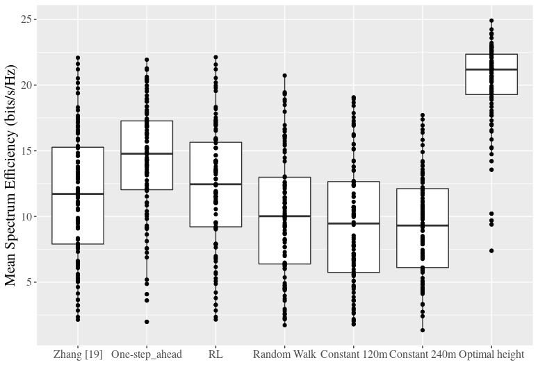
(a) Spectrum efficiency per unit of bandwidth (bits/s/Hz) for low building density

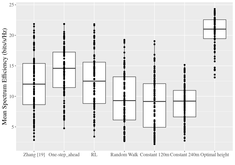
(b) Spectrum efficiency per unit of bandwidth (bits/s/Hz) for medium BS density.

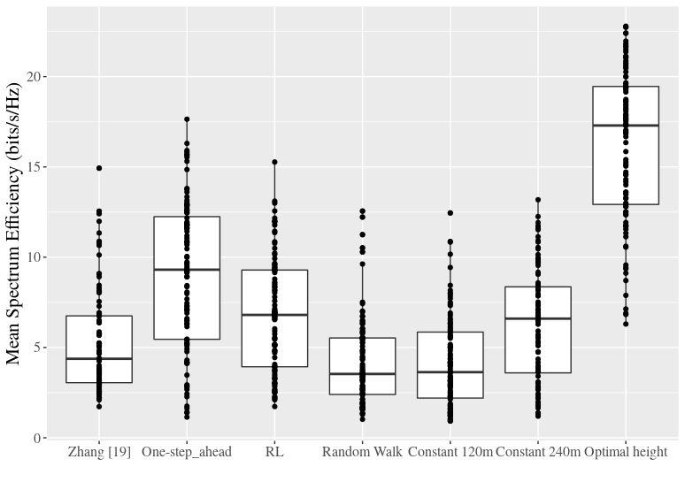
(c) Spectrum efficiency per unit of bandwidth (bits/s/Hz) for high BS density.

Figure 3: Spectrum efficiency per unit of bandwidth (bits/s/Hz) for 3 different BS densities and medium building density.

VI-A Baselines

We choose five different height selection strategies to which we compare performance of our proposed RL algorithm. For the first one, we use the baseline proposed by Zhang [trajec-mobile], which suggests that the UAV maintain the minimum allowed height during its flight. One of the most common approaches to UAV height selection is to maintain a constant height [nallanathan, rami1, reshape, network-adapt], but there is no consensus on which height value to choose. To make a fair comparison, we also benchmark our approach against two constant height values. These heights will be the maximum possible height (120 m), and half of the maximum (60 m). When following these fixed height strategies, the UAV will begin at the minimum height at timestep 1, before increasing its height in each timestep until it reaches the required height, after which it will make no further adjustments.

To confirm that our solution is actually learning based on observed environment information and not acting randomly, we also compare it to a bounded Random walk height selection strategy, in which the UAV in each timestep randomly selects one of three actions: increase the height, decrease the height, or keep the current height. It is bounded as all the solutions and cannot fly outside the allowed flight range.

In order to compare our solution to a more complex baseline, we implement an approach that we call One-step-ahead solution. In the One-step-ahead approach, the UAV knows whether the maximum SINR in the next time step will be found above or below its current height, and will move up or down (in a fixed increment of d = 10 m) depending on this knowledge. To be able to apply the One-step-ahead solution, the UAV needs previous information about the environment; this is not feasible in a real-world application, but we include this to assess whether and by how much such information would improve performance when compared to our RL approach.

We also compare our RL solution with one based on optimal height at each time step as obtained from the real-world dataset. In this approach, it is assumed that the UAV is able to move to any height in the next timestep, without restrictions of $d$. This represents the ideal-case performance which would not be possible in a real-world UAV application.

Bellow are benchmark approaches:

• Zhang [trajec-mobile]: this benchmark proposes that the UAV should maintain the minimal allowed height at all times.

• Constant at 60 m: this benchmark starts at the minimal height, like all others, and then moves up at every step until it achieves 60 m height. After achieving 60 m, the UAV should not move up or down.

• Constant at 120 m: this benchmark starts at the minimal height, like all others, and then moves up at every step until it achieves 120 m height. After achieving 120 m, the UAV should not move up or down.

• Random walk: this benchmark chooses its action randomly at each step.

• Optimal height: this is a reference benchmark of the maximum possible QoS values. In this approach, the UAV does not have any limitations on the maximum height change from step to step and also know which height has the maximum QoS.

• One-step-ahead: this benchmark follows the optimal height next position to decide its next action. If in the next step the optimal height is above the actual height of the UAV, the chosen action will be to move up. If in the next step the optimal height is bellow the actual height of the UAV, the chosen action will be to move down. In case the optimal height in the next step is the same as the actual height, the UAV should not move.

VI-B Spectrum efficiency

In this section we analyse the mean of spectrum efficiency per unit of bandwidth, that is a mean of the spectrum efficiency over an entire episode, for varying BS densities and building densities. We inspect the spectrum efficiency as this is the parameter that we wish to optimise.

VI-B1 Varying BS densities

To demonstrate how the RL solution can have its performance affected by different BS densities, we study in detail three different BS densities $(1,2.5,5)/km^{2}$, denoted as low, medium and high, as illustrated in Figure 3.

Figure 3(a) shows the mean spectrum efficiency per approach. As expected, the optimal height provides much better spectrum efficiency, achieving median of 23 bits/s/Hz. This happens because it does not have any movement restriction, being able to move any distance from step to step. For low BS density, One-step-ahead, Zhang [trajec-mobile] and the proposed RL approach perform similarly, with all archiving median of 20 bits/s/Hz. The constant height at 240 m is the approach with the worse spectrum efficiency, with 15 bits/s/Hz, showing that high heights for low BS density do not perform as good as other approaches do. Constant at 120 m performed slightly worse than the Random walk approach, with median of 18.5 bits/s/Hz and Random walk approach with 19 bits/s/Hz. It is interesting to note that the approaches do not vary much its mean spectrum efficiency, and all have a relatively small first and third quartile of around 2 bits/s/Hz, with exception of Constant at 240 m with 4 bits/s/Hz.

Figure 3(b) shows that our RL approach performs better, 4%, then Zhang [trajec-mobile] for medium BS density, and 26% better than Constant at 120 m, Constant at 240 m and Random walk. It indicates that maintaining higher heights at all times provides worse spectrum efficiency for the medium BS and building densities when compared to the proposed RL approach that adapts the height dynamically to the environment. One-step-ahead showed the best performance compared to the approaches that could only move ”d”, achieving 14.5 bits/s/Hz, showing that for medium BS density having previous knowledge of the radio characteristics of the environment can improve the UAV QoS.

When investigating the high BS density in Figure 3(c), Constant at 120 m and Random walk are the worst solutions achieving 3.5 bits/s/Hz, with the Zhang [trajec-mobile] being slightly better than them, showing that maintaining the lowest altitude for all topologies is not the best approach. The proposed RL approach shows performance comparable to Constant at 240 m, with 4% better performance. Therefore, its third quartile is higher, which means that the RL performed better in more runs. The One-step-ahead approach showed the best performance with its median achieving 9 bits/s/Hz, showing the previous knowledge of the environment can improve UAVs QoS. However, it is unrealistic to expect to have this knowledge for each set of coordinates in the environment.

When analysing a macro view between the different densities, Figure 3 shows that the general mean spectrum efficiency for low BS density is much better than for medium and high BS density, with solutions archiving near 20 bits/s/Hz. We can also analyse that One-step-ahead and the proposed RL solution are always the best approaches for all densities, showing that an intelligent and adaptable decision can provide a good QoS for all densities. Moreover, the proposed RL solution can adapt its response to the environment on the fly without previous knowledge.

VI-B2 Varying building densities

(a) Spectrum efficiency per unit of bandwidth (bits/s/Hz) for low building density

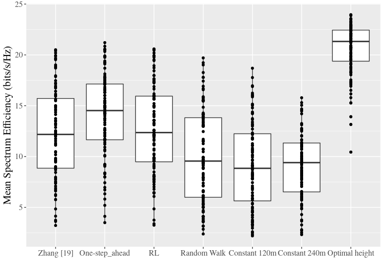
(b) Spectrum efficiency per unit of bandwidth (bits/s/Hz) for high building density.

Figure 4: Spectrum efficiency per unit of bandwidth (bits/s/Hz) for different building densities with medium BS density.

Figure 4 illustrates the spectrum efficiency for low and high building density. In Figure 4(a), the One-step-ahead provides the best approach achieving median of 15 bits/s/Hz, and the proposed RL approach is the second best with 12.5 bits/s/Hz. We can observe that Zhang [trajec-mobile] approach achieves 11.7 bits/s/Hz, that is 6% worse than the proposed RL solution. The Constant at 240 m performs as well as the Constant at 120 m, and both are worse than all other solutions, which show a deterioration for those heights, implying that the UAV would be most of the time in a poor coverage area. Random walk approach performed slightly better then the higher constant approaches, showing that the Random walk movement of the UAV is comparable to maintaining high constant values.

Figure 4(b) illustrates the mean spectrum efficiency for high building density. It shows a similar pattern when compared to the low building density, with One-step-ahead being the best approach and the proposed RL solution being slightly better, 2%, than Zhang [trajec-mobile]. We can conclude that since it has no impact, it is providing an indication that building density is not a factor that needs to be taken account when determining UAV’s height. It shows that that same approach should work in density urban areas and rural ones. As an overall performance between the three different densities, we discovered that the difference in the building density when the UAV is flying above the buildings did not influence the mean spectrum efficiency as the approaches performed similar in all the distributions.

VI-C Height variation

While in the previous section we focus our analyses on the spectrum efficiency of each approach, in this section we inspect in more detail underlying height variations that achieve the discussed performance.

To make a more detailed investigation over the 100 MC trials, Figure 5 illustrates the mean of the heights for different BS and building densities. The constant approaches have no variance on the height after they achieve their constant heights. In Figure 5(a), the average height of the optimal height approach varies with the BS density, being lower for low BS density, and higher for high BS density. As we can notice, the intelligent approaches, One-step-ahead and the proposed RL solution, adapt their altitude to the one that better serves the BS distribution, also increasing its heights when the BS density increases. The Random walk approach, as it does not consider any information of the environment, it also maintains, in average, the same height in all cases.

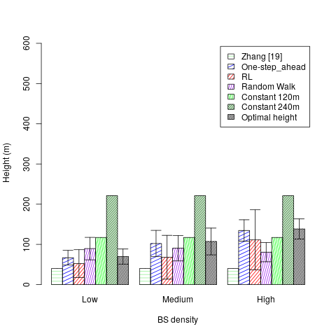
(a) Mean height per BS density.

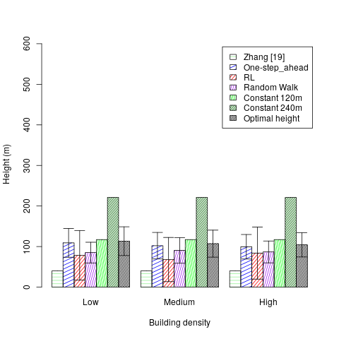
(b) Height per building density.

Figure 5: Height analyses for varying BS and building densities.

When we analyse in Figure 5(b) the height adaptation by the building density, the optimal height is not related with the density. The approaches does not change its mean height considerably during the different building densities. The RL approach varies from 68 m in medium building densities, to 83 m in high building densities.

Observing behaviours for both BS and building densities, we conclude that RL is a competent approach to solve UAV height optimisation. As we can see in Figure 5, the RL solution demonstrated to be learning the best height, resulting in a spectral efficiency improvement. We can also conclude that the RL approach does not make changes on its height at all steps, making intelligent changes when needed and avoiding spending extra energy to move its height at all steps.

VII Real-world Data Evaluation

In this section, we evaluate how our RL approach can adapt the UAV heights with the objective to optimise the total throughput. We first introduce the experimental measurement data-set and then provide a detailed evaluation of the proposed solution using the real-world dataset.

VII-A Experimental measurement Dataset

To evaluate the proposed height adaptation solution, we also use the real-world measurements obtained by a UAV connected to a two-tier cellular network in two different areas of Dublin city’s Smart Docklands, which includes massive Multiple Input Multiple Output (MIMO) macro cells and MIMO small cells. Below, we recap the details of the experiment relevant for our evaluation, while full details of measurements are presented in [measurament].

The experimental cellular network testbed, in which the measurements were conducted, is shown in Figure 6. Connectivity data was collected in two environments: Grand Canal Quay (GCQ) and North Wall Quay (NWQ), as illustrated in Figure 6. The UAV flew at a fixed height back-and-forth in the designated areas. This flight pattern was repeated at 10 meter increments for all heights between 30 and 120 meters (the legal flight ceiling in Dublin).

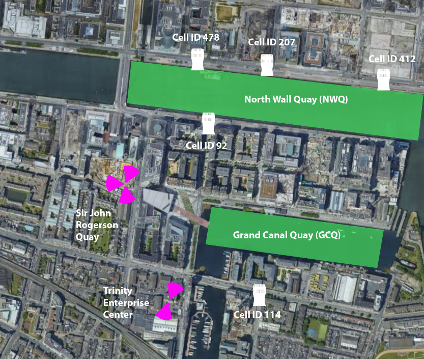
Figure 6: Testbed area from the top. Macro cells are labelled in purple, and small cells are denoted with white icons—the measurement area where the UAV flew is marked in green.

Table III summarises the main characteristics of the experimental environment for NWQ and GCQ. The Table shows: the height of the BS antennas; the velocity the UAV was flying; the total distance the UAV passed in each height; the quantity of measurements reports in each area, denoted as steps; the size of each step in meters; the variation of heights; the building height variation; and the distance $d$ in each scenario. The measurements were reported every 2 seconds most of the time. We also observe that the flight in NWQ resulted in fewer measurements despite being the one where the UAV flies for a longer distance. While a UE is performing handover, it does not sense the spectrum; consequently, it does not report any measurement. In the small cell area, the UAV was performing handovers, which resulted in fewer measurement reports when compared to the macro cell area, where the UAV did not perform measurement reports.

[HTML]C0C0C0 Variable	NWQ Value	GCQ Value
BS height	$6.5m$	$29m$
Speed	4.2 $m/s$	2.6 $m/s$
UAV travel distance	1160 $m$	890 $m$
Steps	161	171
Horizontal step size	7.2m	5.2
Allowed UAV height range	$[30-120]m$	$[20-120]m$
Building height variation	$[20-80]m$	$[20-80]m$
d	$10m$	$10m$

TABLE III: Collection environments.

In order to use the proposed approach with the available real-world data we had slightly modify the definition of an RL agent. In the real-world data the QoS information available is the throughput, so we used this information instead of the spectrum efficiency in the proposed solution. The real-world dataset also had no information about the sensed neighbours, so we do not include this as input of the model. The remainder or the algorithm is exactly the same as in the generated environment. The final state space of the adapted solution is: $s=\{SINR_{t},z_{t},SINR_{t-1},z_{t-1},a_{t-1},r_{t-1},SINR_{t-2},z_{t-2}$ at-2,rt-2,SINRt-3,zt-3