A semi-linear wave model for critical collapse

Abstract

In spherical symmetry compelling numerical evidence suggests that in general relativity solutions near the threshold of black hole formation exhibit critical behavior. One aspect of this is that threshold solutions themselves are self-similar and are, in a certain sense, unique. To an extent yet to be fully understood, the same phenomena persist beyond spherical symmetry. It is therefore desirable to construct models that exhibit such symmetry at the threshold of blow-up. Starting with deformations of the wave equation, we discuss models which have discretely self-similar threshold solutions. We study threshold solutions in the past light cone of the blow-up point. In spherical symmetry there is a sense in which a unique critical solution exists. Spherical numerical evolutions are also presented for more general models, and exhibit similar behavior. Away from spherical symmetry threshold solutions attain more freedom. Different topologies of blow-up are possible, and even locally the critical solution needs reinterpretation as a parameterized family.

I Introduction

The veracity of the weak and strong cosmic censorship conjectures is of monumental importance in classical $3+1$ dimensional gravity. Of these, the weak cosmic censorship conjecture can be thought of informally as the statement that, given generic asymptotically flat initial data, the resulting solution will exist globally outside of a black hole region Penrose (1969); Christodoulou (1999). Strong cosmic censorship is likewise the conjecture of uniqueness of solutions emanating from generic initial data, and is directly related to regularity of solutions at blow-up. A natural role for numerical relativity in this context is in the construction of potential counterexamples. A hope might be to give convincing evidence that an open set of initial data do not have complete black hole exteriors, or are sufficiently regular at blow-up so that they may be extended non-uniquely.

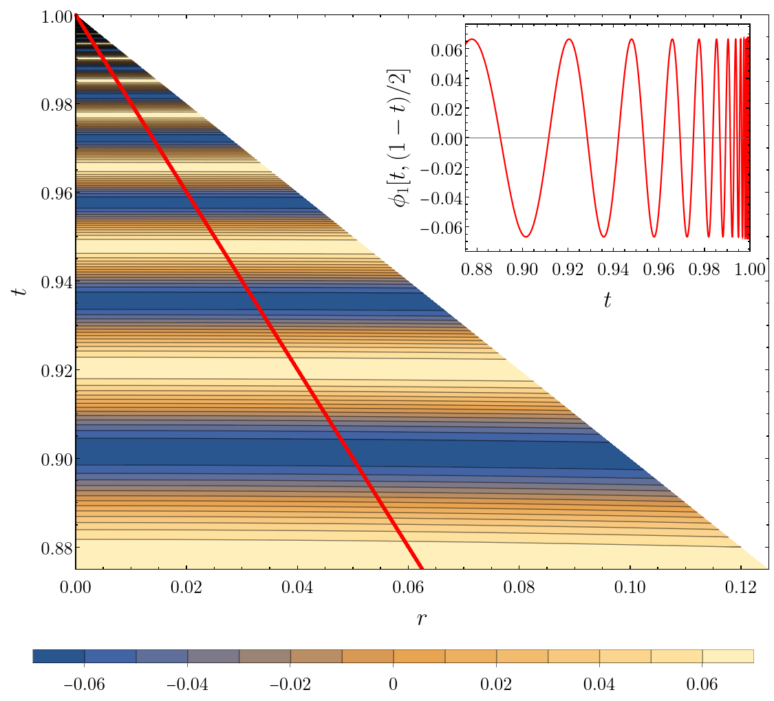
Figure 1: A contour plot of a threshold solution of model 3 with $A_{3}=1/15$, see Eqn. (III). The parameter here was chosen simply for clarity of plotting. This threshold solution blows up in $H^{1}$ (and not in $L^{2}$) in a discretely self-similar fashion at $(t_{\star},r_{\star})=(1,0)$. In the inset the solution is plotted along the red curve $t+2r(t)=1$ indicated in the main plot. The figure is naturally compared with Fig. $1$ of Reiterer and Trubowitz (2019).

One strategy to try and construct such extreme spacetimes is the following: consider a one-parameter family of initial data such that small values of the (strength) parameter result in data close to flat-space, with larger values being more and more deformed. Then tune that strength parameter to the threshold of black hole formation. Starting with the pioneering work of Choptuik Choptuik (1993), studies along these lines in spherical symmetry revealed behavior which has since come to be known as critical phenomena in gravitational collapse Gundlach and Martín-García (2007). In short, it has been found that for a given family there is, in a sense, a single solution lying between dispersion and collapse to form a black hole. Numerical evidence suggests that these solutions have naked singularities, but these are not considered true counterexamples to the cosmic censorship because the phenomena occurs only by fine-tuning the initial data. These threshold solutions are fascinating. Empirically, they are either continuously or discretely self-similar, and, remarkably, for a given model appear to be unique, in the sense that all families of initial data exhibit the same threshold solution, called the critical solution, and are thus in some sense as close as possible to being attractors in solution space. Consequently, when considered as a function of the strength parameter, solutions naturally give rise to power law behavior near the threshold. For example, when the critical solution is discretely self-similar, the maximum of any non-vanishing curvature scalar, viewed as a function of distance from the threshold in phase space, follows a power law with a superposed periodic wiggle Gundlach (1997); Hod and Piran (1997); Garfinkle and Duncan (1998). Beyond spherical symmetry similar behavior has also been observed, although typically with features that have yet to be persuasively explained. For example in the collapse of electromagnetic waves Baumgarte et al. (2019), threshold solutions appear to be only approximately self-similar.

Much of the picture of critical collapse described above was formed through a combination of the empirical findings of numerical studies and thoughtful heuristic modeling. To understand what might be shown rigorously it is therefore desirable to construct maximally simple models that capture the qualitative behavior near the threshold of blow-up. Various such investigations have been made in the literature Liebling (2002); Bizon et al. (2004); Liebling (2005); Bizoń et al. (2007); Bizon and Zenginoglu (2009), but all so far exhibit continuous, rather than discrete self-similarity. From the point of view of nonlinear PDEs we therefore seek a simple system that admits a small-data global existence result, but with large data breaking down, and a unique discretely self-similar critical solution at the threshold between the two regimes. Illustrative would furthermore be if, just as the system,

$$\square\phi=\nabla_{a}\phi\nabla^{a}\phi\,,$$ (1)

can be used to motivate the utility of the classical null condition Klainerman (1980), the model were to indicate the structural form of nonlinear terms that generate self-similar critical solutions. We denote by $\nabla$ the Levi-Civita derivative compatible with $\eta_{ab}$, the Minkowski metric, and $\square$ the flat space d’Alembertian. The first aim of this work is to give, for the first time, such a model. In what follows we therefore present a number of different toys. With the simplest parameter choice, one of our models is

$$\square\phi+\frac{\phi-\sqrt{1-\phi^{2}}}{1-\phi^{2}}\nabla_{a}\phi\nabla^{a}\phi=0\,.$$ (2)

In Figure 1 we plot a spherical solution to the associated model equation at the threshold of blow-up (albeit with slightly different parameters for the purposes of plotting) in the past light-cone of the blow-up point.

We are furthermore interested in the properties of solutions near blow-up and in the status of conjectures related to cosmic censorship both in and beyond spherical symmetry. All of the models we study, like (2), are semi-linear or equivalent to a semi-linear PDE. That is, there is no nonlinearity whatsoever in the principal part. The principal part is furthermore taken to be the d’Alembert operator associated with the Minkowski metric. With the metric so fixed, there are no notions of either trapped surface, or black hole formation intrinsic to the model. Therefore, in any setup with this restriction, if blow-up is present without fine-tuning initial data, the obvious conjecture directly analogous to weak cosmic censorship must be false. Our focus is instead on the nature of solutions at the threshold of blow-up, and the extent to which critical behavior is obtained for solutions nearby in phase space.

The paper is structured as follows. In section II we discuss different notions of blow-up and self-similarity. Then in section III we explain the construction of our various models. In section IV we study the behavior of threshold and near-threshold solutions. Afterwards, we restrict to spherical symmetry and present a set of numerical evolutions in section V. We conclude in section VI.

II Self-similar functions

Solutions to our models either live forever or terminate at some finite time. The manner in which solutions blow up in our models splits into two categories depending on the model. Either just first derivatives, or the field itself explodes pointwise. Each of these has an obvious, although inequivalent, analogue in $L^{2}$-like norms. Solutions at the threshold of blow-up may exhibit more structure, described in many cases by self-similarity, a special class of scale invariance. Likewise, in our examples two types of self-similarity, discrete and continuous, manifest. Since these threshold solutions are just examples of blow-up, there must then be a relationship between these notions, which we discuss in this section.

Notions of blow-up.

The choice of a function space in which mathematical results are formulated and proven is subtle, but for our models a simple overview will suffice. A function $f(t,x^{i})$ is said to be in $L^{2}$ at instant $t$ if the integral

$$||f||_{L^{2}}\equiv\left(\int_{\mathcal{D}[f(t,\cdot)]}\textrm{d}\Sigma\left|f(t,x^{i})\right|^{2}\right)^{1/2}$$ (3)

exists and is finite, where $\mathcal{D}[f(t,\cdot)]$ is the domain of $f(t,x^{i})$. Throughout, the coordinates $t,x^{i}$ are taken to be global inertial on Minkowski and $\textrm{d}\Sigma$ denotes the natural volume form induced in level sets of $t$. Another norm that appears in the study of wave equations is given by

$$||f||_{H^{1}}\equiv$$

$$\left(\int_{\mathcal{D}[f(t,\cdot)]}\textrm{d}\Sigma\,\Big{(}\left|f(t,x^{i})\right|^{2}+\sum_{i}\left|\partial_{i}f(t,x^{i})\right|^{2}\Big{)}\right)^{1/2}\,.$$ (4)

When this quantity is finite we will colloquially refer to the function as being $H^{1}$. Here and in what follows $\partial_{i}$ denotes the partial derivative $\partial/\partial{x^{i}}$. More generally, a function $f(t,x^{i})$ is said to be in the Sobolev space $H^{k}$ at instant $t$ if the norm Ringström (2009)

$$||f||_{H^{k}}\equiv\left(\int_{\mathcal{D}[f(t,\cdot)]}\textrm{d}\Sigma\sum_{|\alpha|\leq k}\left|\partial^{\alpha}_{i}f(t,x^{i})\right|^{2}\right)^{1/2}$$ (5)

is finite. In the last expression, we are using the multi-index notation with the $3$-tuple $\alpha=(\alpha_{1},\alpha_{2},\alpha_{3})$ of non-negative integers, where $|\alpha|=\alpha_{1}+\alpha_{2}+\alpha_{3}$ and $\partial_{i}^{\alpha}f\equiv\partial_{x}^{\alpha_{1}}\partial_{y}^{\alpha_{2}}\partial_{z}^{\alpha_{3}}f$. Note that $H^{0}\equiv L^{2}$. We additionally consider the $E^{1}$-norm Klainerman (1980)

$$||f||_{E^{1}}\equiv$$

$$\left(\int_{\mathcal{D}[f(t,\cdot)]}\textrm{d}\Sigma\,\Big{(}\left|\partial_{t}f(t,x^{i})\right|^{2}+\sum_{i}\left|\partial_{i}f(t,x^{i})\right|^{2}\Big{)}\right)^{1/2}\,,$$ (6)

which is perhaps the norm that appears most naturally for wave equations. When a function which is initially in $H^{k}$ ($E^{1}$) fails to be so at some instant $t^{\prime}$, we say that it “blows up” in $H^{k}$ ($E^{1}$) at that instant $t^{\prime}$. Clearly, if a function blows up in $H^{k}$, it blows up also in $H^{k^{\prime}}$ with $k^{\prime}>k$.

We might like to restrict our attention exclusively to classical solutions with bounded derivatives (called $C_{b}^{k}$) and discuss blow-up exclusively in terms of the field or derivatives thereof. Alternatively, we may want to consider the function space $L^{\infty}$ of measurable bounded functions; this space contains and has the same norm of $C_{b}^{0}$. However, besides the inconvenient fact that proofs of existence and so forth do not naturally appear in these spaces, the formulation of the weak cosmic censorship itself Christodoulou (1999) is given in terms of local $L^{2}$ integrability of the connection coefficients. Intuitively this makes sense, because we can introduce local inertial coordinates at any point, and so if some blow-up occurs and is unavoidable we might expect it to be associated with at least one derivative of the metric, and hence the connection appears naturally. From a modeling point of view, we are therefore more interested in finding semi-linear wave equations with blow-up in $E^{1}$ rather than in $L^{2}$.

Self-similar functions.

The notion of self-similarity has to do with invariance under certain scale transformations. We consider two kinds of self-similarity; continuous (CSS) and discrete (DSS). A scalar function $f$ is said to be CSS if there exists a coordinate system $(t,x^{i})$ and a $\nu\in\mathbb{R}$ such that

$$f(\lambda t,\lambda x^{i})=\lambda^{\nu}f(t,x^{i})\,,$$ (7)

for any $\lambda>0$. Notice that we have chosen our coordinates so that the origin coincides with the center of the symmetry. When $\nu$ is an integer, $f$ is also called a homogeneous function of degree $\nu$. On the other hand, a function $f$ is said to be DSS if there exists coordinate system $(t,x^{i})$, a $\nu\in\mathbb{R}$, and some $\Delta>0$ such that (7) holds for $\lambda=e^{-m\Delta}$, with any $m\in\mathbb{Z}$. Thus, DSS functions have a fractal-type behavior under scale transformations. The condition (7) is often expressed in similarity coordinates $(T,X^{i})=(-\log|t|,x^{i}/t)$ as

$$f(T+\tau,X^{i})=e^{-\nu\tau}f(T,X^{i})\,,$$ (8)

where $\tau=-\log\lambda$. In the case of DSS functions the last condition is satisfied for $\tau=m\Delta$.

Self-similarity and blow-up.

Interestingly, self-similar functions offer special examples of blow-up, either pointwise or under some integral norm. For example, a CSS function satisfying (7) – with $x^{i}$ the canonical Cartesian coordinates – satisfies also

$$\int_{\mathbb{R}^{3}}\textrm{d}\Sigma\sum_{|\alpha|=k}\left|\partial^{\alpha}_{i}f(t,x^{i})\right|^{2}=$$

$$\frac{1}{\lambda^{2(\nu-k+3/2)}}\int_{\mathbb{R}^{3}}\textrm{d}\Sigma\sum_{|\alpha|=k}\left|\partial^{\alpha}_{i}f(\lambda t,x^{i})\right|^{2},$$ (9)

with any $\lambda$. Here we are assuming that the domain of $f$ is $\mathbb{R}^{3}$, except (possibly) a set of zero measure. Choosing $\lambda=1/|t|$ we see that for $t<0$

$$\int_{\mathbb{R}^{3}}\textrm{d}\Sigma\sum_{|\alpha|=k}\left|\partial^{\alpha}_{i}f(t,x^{i})\right|^{2}=$$

$$\frac{1}{|t|^{2(k-\nu-3/2)}}\int_{\mathbb{R}^{3}}\textrm{d}\Sigma\sum_{|\alpha|=k}\left|\partial^{\alpha}_{i}f(-1,x^{i})\right|^{2},$$ (10)

Thus, a nontrivial CSS function with $\nu\leq-3/2+k$ cannot be in $H^{k}$ for all times; if it is in $H^{k}$ at a particular instant $t<0$, it must blow up at $t=0$. It is easy to see that the same argument goes through for CSS functions in $E^{1}$; if a non-trivial CSS function with $\nu\leq-1/2$ is in $E^{1}$ at a particular instant $t<0$, it must blow up at $t=0$. A CSS function satisfies

$$\partial_{t}^{\alpha}f(t,x^{i}) =\frac{1}{\lambda^{\nu-k}}\,\partial_{\lambda t}^{\alpha}f(\lambda t,\lambda x^{i})\,,\qquad|\alpha|=k\,,$$

$$\partial_{x^{i}}^{\alpha}f(t,x^{i}) =\frac{1}{\lambda^{\nu-k}}\,\partial_{\lambda x^{i}}^{\alpha}f(\lambda t,\lambda x^{i})\,,\qquad|\alpha|=k\,.$$ (11)

with any $\lambda$. Choosing again $\lambda=1/|t|$, we obtain

$$\partial_{t}^{\alpha}f(t,x^{i}) =\frac{1}{|t|^{k-\nu}}\,\partial_{\lambda t}^{\alpha}f(\lambda t,\lambda x^{i})_{|(-1,x^{i}/|t|)}\,,\quad|\alpha|=k\,,$$

$$\partial_{x^{i}}^{\alpha}f(t,x^{i}) =\frac{1}{|t|^{k-\nu}}\,\partial_{\lambda x^{i}}^{\alpha}f(\lambda t,\lambda x^{i})_{|(-1,x^{i}/|t|)}\,,\quad|\alpha|=k\,.$$ (12)

So, a CSS function with $\nu<k$ cannot be in $C_{b}^{k}$ for all times; if it is in $C_{b}^{k}$ at a particular instant $t<0$, it must blow up at $t=0$. The two arguments above can be easily extended to DSS functions with the same bounds on $\nu$ by taking the limit $t\to 0^{-}$ through a sequence $t_{m}=-1/\lambda_{m}=-e^{-m\Delta}$. Note that DSS functions satisfy (II) and (II) for a discrete set of values of $\lambda$. The results of this section are summarized in Tab. 1.

$H^{k}$	$E^{1}$	$C_{b}^{k}$
$\nu\leq-3/2+k$	$\nu\leq-1/2$	$\nu<k$

Table 1: A CSS or DSS function with degree $\nu$ (see Eqn. (7)) must blow up in a given function norm (first line) if the associated condition in $\nu$ (second line) is satisfied.

Sobolev embedding.

It can be shown (for details see Theorem 6.5 in Ringström (2009)) that, for each $k$ a non-negative integer and $s>k+3/2$, there is a constant $c$ such that

$$||f||_{C_{b}^{k}}\leq c\,||f||_{H^{s}}\,,$$ (13)

with $f$ an arbitrary function. In particular, for $k=0$ and $s=2$,

$$||f||_{C_{b}^{0}}\leq c\,||f||_{H^{2}}\,.$$ (14)

This implies that if a function blows up in $C_{b}^{0}$, it also blows up in $H^{2}$. Since the $C_{b}^{0}$-norm is equal to the $L^{\infty}$-norm, if a function blows up in $L^{\infty}$ it also blows up in $H^{2}$.

III Model Equations

In this section we present a simple method to generate nonlinear wave equations with analytically known solutions, which we state explicitly in terms of partial waves. We then list the specific models used throughout the article. Some, but not all, of our models follow this procedure directly.

The wave equation and partial wave solutions.

Let $(r,\theta^{A})$ be spherical polar coordinates built from $x^{i}$ in the usual manner. In these coordinates the flat-space wave equation is,

$$\square\varphi\equiv-\partial_{t}^{2}\varphi+\partial_{r}^{2}\varphi+\tfrac{2}{r}\partial_{r}\varphi+\not{\Delta}\varphi=0\,,$$ (15)

with $\not{\Delta}$ the standard Laplacian on the round two-sphere of area radius $r$. The general solution can be written in terms of partial waves $\varphi_{lm}(t,r)$, with the full solution constructed as

$$\varphi=\sum_{l=0}^{\infty}\sum_{m=-l}^{l}\varphi_{lm}(t,r)Y_{lm}(\theta^{A})\,,$$ (16)

with $Y_{lm}$ the standard spherical harmonics. Each partial wave solves the associated equation,

$$-\partial_{t}^{2}\varphi_{lm}+\partial_{r}^{2}\varphi_{lm}+\tfrac{2}{r}\partial_{r}\varphi_{lm}-\tfrac{l(l+1)}{r^{2}}\varphi_{lm}=0\,.$$ (17)

For our needs a convenient representation for the exact regular solution of this equation is Gundlach et al. (1994),

$$\varphi_{lm}=\sum_{k=0}^{l}\frac{(k+l)!}{2^{k}k!(l-k)!}\frac{1}{r^{k+1}}[F^{l-k}(u)-(-1)^{l-k}F^{l-k}(v)]\,,$$ (18)

with retarded time $u=t-r$ and advanced time $v=t+r$ defined in the usual way, and $F$ a real-valued function which we take to decay at large argument, and which is determined by the desired initial data for the partial wave and its time derivative.

Deformation-functions.

To generate nonlinear equations, we use the deformed scalar field $\phi\equiv D(\varphi)$, which, whenever $\varphi$ satisfies (15), must solve

$$\square\phi-\chi\nabla_{a}\phi\nabla^{a}\phi=0\,,$$ (19)

where $\nabla_{a}\phi\nabla^{a}\phi\equiv-(\partial_{t}\phi)^{2}+(\partial_{r}\phi)^{2}+\not{\nabla}_{a}\phi\not{\nabla}^{a}\phi$ and $\not{\nabla}$ denotes the covariant derivative induced by $\eta_{ab}$ on the two-spheres of constant $u$ and $v$. The deformation function $D$ is taken to be twice continuously differentiable and such that

$$\chi=\tfrac{D^{\prime\prime}}{D^{\prime 2}}$$ (20)

is single-valued when viewed as a function of $\phi$. We require moreover that $D(\varphi)\simeq\varphi$ for small $\varphi$. This implies, by construction, that the model has global solutions for small initial data, that analytic solutions can be trivially constructed using (18). Moreover the manner of blow up for larger data, should that occur, is determined by the specific choice of $D$. We will see below that when the deformation function involves a periodic function this construction has to be adjusted slightly, but the core idea is unaltered. Below we list the models studied in the article.

Model $\bm{1}$.

This model is generated by the deformation function

$$\phi=D(\varphi)\equiv A_{1}^{-1}\log(1+A_{1}\varphi)\,,$$ (21)

which results in the nonlinear wave equation

$$\square\phi+A_{1}\nabla_{a}\phi\nabla^{a}\phi=0\,.$$ (22)

The parameter $A_{1}$ is a real constant that we are free to choose. Similar parameters appear in the subsequent models. This is the classical example of Nirenberg which motivates the classical null condition for nonlinear wave equations and was discussed in Klainerman (1980). We use it primarily to determine reliability of our code in preparation for solving models that do not arise as deformations of the wave equation.

Model $\bm{2}$.

Ultimately we are interested not in equations that arise by manipulation of the wave equation, but those that appear in physical applications in GR. To build at least some confidence that the properties of threshold solutions of the former are not peculiar to those specific models, we will compute numerical solutions for systems that cannot be constructed in the same way. The first of these is a modification extension of model $1$ to a system of two coupled scalar fields. It is described by the system

$$\square\phi_{1}+A_{2}\nabla_{a}\phi_{2}\nabla^{a}\phi_{2}=0\,,$$

$$\square\phi_{2}+B_{2}\nabla_{a}\phi_{1}\nabla^{a}\phi_{1}=0\,.$$ (23)

Here we do not know solutions analytically, but in the special case that $A_{2}=B_{2}=A_{1}$ they coincide with those of (22) provided that $\phi_{1}$ and $\phi_{2}$ and their time derivatives agree as functions.

Model $\bm{3}$.

Looking at plots of the Choptuik solution, for example Figs. $3$ and $4$ of Baumgarte (2018), one is starkly reminded of the topologists sine curve. We therefore want to consider deformations involving periodic functions. To avoid subtleties with branch-cuts however we adjust the construction made in (19) as follows,

$$\phi_{1}=D_{1}(\varphi)\equiv A_{3}\sin\left[A_{3}^{-1}\log(1+\varphi)\right]\,,$$

$$\phi_{2}=D_{2}(\varphi)\equiv A_{3}\cos\left[A_{3}^{-1}\log(1+\varphi)\right]\,.$$ (24)

Although these deformations are not globally invertible, $D_{1}^{\prime\prime}/D_{1}^{\prime 2}$ and $D_{2}^{\prime\prime}/D_{2}^{\prime 2}$ are single-valued functions of both $\phi_{1}$ and $\phi_{2}$. Together these generate the nonlinear coupled equations

$$\square\phi_{1}+\frac{\phi_{1}+A_{3}\phi_{2}}{A_{3}^{2}-\phi_{1}^{2}}\nabla_{a}\phi_{1}\nabla^{a}\phi_{1}=0\,,$$

$$\square\phi_{2}+\frac{\phi_{2}-A_{3}\phi_{1}}{A_{3}^{2}-\phi_{2}^{2}}\nabla_{a}\phi_{2}\nabla^{a}\phi_{2}=0\,,$$ (25)

with the algebraic constraint $\phi_{1}^{2}+\phi_{2}^{2}=A_{3}^{2}$. Using the constraint we obtain

$$\frac{\nabla_{a}\phi_{1}\nabla^{a}\phi_{1}}{A_{3}^{2}-\phi_{2}^{2}}-\frac{\nabla_{a}\phi_{2}\nabla^{a}\phi_{2}}{A_{3}^{2}-\phi_{1}^{2}}=0\,,$$ (26)

and also

$$\phi_{1}\square\phi_{1}+\phi_{2}\square\phi_{2}+\nabla_{a}\phi_{1}\nabla^{a}\phi_{1}+\nabla_{a}\phi_{2}\nabla^{a}\phi_{2} =0\,,$$ (27)

which, with system (III), results in,

$$\nabla_{a}\phi_{1}\nabla^{a}\phi_{1}+\nabla_{a}\phi_{2}\nabla^{a}\phi_{2}=A_{3}^{2}\frac{\nabla_{a}\phi_{1}\nabla^{a}\phi_{1}}{A_{3}^{2}-\phi_{2}^{2}}.$$ (28)

Using this relation it is easy to see that system (III), subject to the algebraic constraint, is equivalent to

$$\square\phi_{1}+A_{3}^{-2}\left(\phi_{1}+A_{3}\phi_{2}\right)\left(\nabla_{a}\phi_{1}\nabla^{a}\phi_{1}+\nabla_{a}\phi_{2}\nabla^{a}\phi_{2}\right)=0\,,$$

$$\square\phi_{2}+A_{3}^{-2}\left(\phi_{2}-A_{3}\phi_{1}\right)\left(\nabla_{a}\phi_{1}\nabla^{a}\phi_{1}+\nabla_{a}\phi_{2}\nabla^{a}\phi_{2}\right)=0\,.$$ (29)

For the Cauchy problem, solutions with initial data satisfying the constraint will be of the form (III), and thus satisfy the constraint everywhere for all times. For the initial boundary value problem boundary conditions must be constraint preserving. At the continuum level there is thus no clear advantage of (III) over (III), but crucially for numerical approximation we avoid the explicit poles present in the latter. By using the constraint to eradicate either $\phi_{1}$ or $\phi_{2}$ in Eqn. (III), we see that the fields satisfy equations similar to (2).

Model $\bm{4}$.

Just as we view model $2$ as an extension model $1$, in model $4$ we extend model $3$ by dropping the algebraic constraint on $\phi_{1}^{2}+\phi_{2}^{2}$. We simultaneously adjust the equations of motion to

$$\square\phi_{1}+A_{4}^{-2}\left(\phi_{1}+A_{4}\phi_{2}\right)\left(\nabla_{a}\phi_{1}\nabla^{a}\phi_{1}+\nabla_{a}\phi_{2}\nabla^{a}\phi_{2}\right)=0\,,$$

$$\square\phi_{2}+B_{4}^{-2}\left(\phi_{2}-B_{4}\phi_{1}\right)\left(\nabla_{a}\phi_{1}\nabla^{a}\phi_{1}+\nabla_{a}\phi_{2}\nabla^{a}\phi_{2}\right)=0\,.$$ (30)

Again, since this model was not obtained from a deformation of the wave equation, solutions of this system are not known analytically in general, but are coincident when the constraint is satisfied and $A_{4}=B_{4}$. Blow-up solutions will be investigated carefully in the section IV, but it is already obvious that blow-up solutions for model $3$ will be oscillatory in nature. The key question here, which we examine numerically in section V, is whether or not this behavior persists generically with the present model.

Model $\bm{5}$.

Returning to the general deformation function, we can define the conformal metric $\tilde{\eta}_{ab}=\Omega^{2}\eta_{ab}$ with conformal factor $\Omega^{-2}=\partial_{\varphi}D$ viewed now as a function of $\phi$. We denote the inverse conformal metric by $\tilde{\eta}^{ab}$ and the associated covariant derivative by $\tilde{\nabla}_{a}$. In these terms the general deformation equation (19) can be rewritten as,

$$\tilde{\Box}\phi\equiv\tilde{\eta}^{ab}\tilde{\nabla}_{a}\tilde{\nabla}_{b}\phi=0\,.$$ (31)

It follows immediately that the deformed wave equation admits the standard stress-energy,

$$T_{ab}[\phi] =\tilde{\nabla}_{a}\phi\tilde{\nabla}_{b}\phi-\tfrac{1}{2}\tilde{\eta}_{ab}\tilde{\nabla}^{c}\phi\tilde{\nabla}_{c}\phi\,,$$ (32)

where, as is conventional, indices on the conformal covariant derivatives were raised using the conformal metric. The stress-energy (32) is of course covariantly conserved $\tilde{\nabla}^{b}T_{ab}[\phi]=0$. In this manner we have rewritten our original model in a clean geometric form that resulted in a quasilinear equation. This reformulation by itself is not particularly helpful, but in the future the conserved energy will certainly be useful in proving the findings of this paper rigorously. This construction also allows us to build more general ‘DSS’ type models too. Let $\phi=\phi_{0}$, and suppose that the original deformation function $D$ is monotonic increasing on its domain. Inspired by (III), set

$$\phi_{1} =P_{1}(\phi_{0})\,,\qquad\phi_{2}=P_{2}(\phi_{0})\,,$$ (33)

where $P_{1}$ and $P_{2}$ are any periodic functions that satisfy

$$P_{1}^{2}+P_{2}^{2}=\delta^{2}\,,\qquad P_{1}^{\prime 2}+P_{2}^{\prime 2}=\varepsilon^{2}\,,$$ (34)

with $\delta$ and $\varepsilon$ positive functions of $\phi_{0}$ uniformly bounded above and below away from $0$. Computations very similar to those for model $3$ in the build up to (III) then reveal the regularized equations of motion,

$$\tilde{\Box}\phi_{1}-\varepsilon^{-2}P_{1}^{\prime\prime}(\phi_{0})\big{(}\tilde{\nabla}^{a}\phi_{1}\tilde{\nabla}_{a}\phi_{1}+\tilde{\nabla}^{a}\phi_{2}\tilde{\nabla}_{a}\phi_{2}\big{)}=0\,,$$

$$\tilde{\Box}\phi_{2}-\varepsilon^{-2}P_{2}^{\prime\prime}(\phi_{0})\big{(}\tilde{\nabla}^{a}\phi_{1}\tilde{\nabla}_{a}\phi_{1}+\tilde{\nabla}^{a}\phi_{2}\tilde{\nabla}_{a}\phi_{2}\big{)}=0\,.$$ (35)

These equations can be solved alongside (31) for a complete model. The fields $\phi_{1}$ and $\phi_{2}$ have a combined conserved stress-energy that can again be obtained naturally by a conformal transformation. This model has the disadvantage of requiring more fields, but is more robust than model $3$, because it grants a large amount of freedom in choosing a compactifying function. A shortcoming of using (31) with (35) is that the coupling between the fields is one-directional, which makes it impossible, when choosing initial data, that violate the various constraints between the different fields, to seed non-trivial evolution in $\phi_{0}$ from $\phi_{1}$ and $\phi_{2}$. A final modification can be made to sidestep this. Using

$$\varepsilon^{2}\tilde{\nabla}^{a}\phi_{0}\tilde{\nabla}_{a}\phi_{0}=\tilde{\nabla}^{a}\phi_{1}\tilde{\nabla}_{a}\phi_{1}+\tilde{\nabla}^{a}\phi_{2}\tilde{\nabla}_{a}\phi_{2}\,,$$ (36)

Eqn. (31) can be rewritten as,

$$\hat{\Box}\phi_{0}-\varepsilon^{-2}\chi\big{(}\tilde{\nabla}^{a}\phi_{1}\tilde{\nabla}_{a}\phi_{1}+\tilde{\nabla}^{a}\phi_{2}\tilde{\nabla}_{a}\phi_{2}\big{)}=0\,,$$ (37)

where $\hat{\Box}\phi_{0}\equiv\tilde{\eta}^{ab}\nabla_{a}\nabla_{b}\phi_{0}$ denotes the reduced wave operator associated with $\tilde{\eta}_{ab}$, and $\chi$ is again to be viewed as a function of $\phi_{0}$. Interestingly, the combined system (35),(37) admits a natural analogy with GR. The fields $\phi_{1},\phi_{2}$ are akin to some field theory matter and, since it is required in building $\tilde{\eta}_{ab}$, the field $\phi_{0}$ to a metric component.

IV Criticality, regularity and the threshold of blow-up

In this section we focus on nonlinear equations, as exemplified by models $1$ and $3$, that are generated by a deformation of the wave equation. We examine the extent to which threshold solutions and those in a neighborhood of the threshold in phase space exhibit a behavior like that in gravitational collapse. We start with spherical solutions and then move on to the more general setting.

Bounds and blow-up in spherical symmetry.

We want to establish that spherical threshold solutions blow up at the origin. We start with solutions to the wave equation. In this context the d’Alembert solution (18) takes the well-known form

$$\varphi =\frac{1}{r}\,[F(t+r)-F(t-r)]\,.$$ (38)

Consider a subset $\{\varphi_{\star}(t,r)\}$ of the solutions (38), such that for $t<t_{\star}$, we have $\varphi_{\star}(t,r)>\xi_{\star}$, some constant, and $\varphi_{\star}(t_{\star},r_{\star})=\xi_{\star}$ is a local minimum. Loosely speaking we may think of the point $(t_{\star},r_{\star})$ as the location of blow-up in the deformed equation, so that the label $\star$, somewhat prejudicially, stands for “critical”. This minimum must be attained at the origin, $r_{\star}=0$. To see this, suppose on the contrary that $r_{\star}>0$. Since $(t_{\star},r_{\star})$ is a local extremum we have,

$$r_{\star}\left[F_{\star}^{\prime}(t_{\star}+r_{\star})+F_{\star}^{\prime}(t_{\star}-r_{\star})\right] =F_{\star}(t_{\star}+r_{\star})-F_{\star}(t_{\star}-r_{\star})\,,$$

$$F_{\star}^{\prime}(t_{\star}+r_{\star}) =F_{\star}^{\prime}(t_{\star}-r_{\star})\,,$$ (39)

which implies that

$$\varphi_{\star}(t_{\star},r_{\star})=2F_{\star}^{\prime}(t_{\star}-r_{\star})=\xi_{\star}\,.$$ (40)

At the origin however we have

$$\varphi_{\star}(t,0)=2F_{\star}^{\prime}(t)\,,$$ (41)

which gives

$$\varphi_{\star}(t_{\star}-r_{\star},0)=\varphi_{\star}(t_{\star},r_{\star})=\xi_{\star}\,.$$ (42)

By assumption $r_{\star}>0$, so this contradicts the assumption that $\varphi_{\star}(t,0)>\xi_{\star}$ for $t<t_{\star}$. Thus we have shown that $r_{\star}=0$. Consequently the global minimum of a spherical solution to the wave equation occurs at the origin. Consider now a compactifying deformation function $D\left[\varphi\right]=\mathcal{C}\left(\varphi\right)$, with $\mathcal{C}(\varphi)$ defined on $\varphi>\xi_{\star}$ and such that we have the blow-up

$$\lim_{\varphi\to\xi_{\star}}\mathcal{C}(\varphi)=\infty.$$ (43)

Recall from Section III that we additionally require $\mathcal{C}(\varphi)\simeq\varphi$ for small $\varphi$. For a one-parameter family of initial data, the solutions of Eqn. (19) at the threshold between global existence and blow-up in are of the form $\phi_{\star}(t,r)\equiv\mathcal{C}\left[\varphi_{\star}(t,r)\right]$. These are called threshold solutions, and by the previous discussion must blow up at $(t_{\star},0)$.

Criticality of spherical threshold solutions.

Interestingly, the threshold solutions of our deformation models are universal in the sense that the form of their blow-up near $(t_{\star},0)$ is independent of the initial conditions and, thus, of the family of initial data considered. We therefore call this “late time” universal solution a critical solution. To illustrate this notice that the original solution to the wave equation satisfies,

$$\lim_{(t,r)\to(t_{\star},0)}\varphi_{\star}(t,r)\sim\xi_{\star}+\tfrac{1}{2}\partial_{t}^{2}\varphi_{\star}(t_{\star},0)\left(t_{\star}-t\right)^{2}$$

$$\qquad-\tfrac{1}{2}\partial_{t}\partial_{r}\varphi_{\star}(t_{\star},0)\left(t_{\star}-t\right)r+\tfrac{1}{2}\partial_{r}^{2}\varphi_{\star}(t_{\star},0)r^{2}\,.$$ (44)

Moreover, it is easy to show that $\partial_{t}\partial_{r}\varphi(t,0)=0$ and $\partial^{2}_{t}\varphi(t,0)=3\partial^{2}_{r}\varphi(t,0)=2F^{\prime\prime\prime}(t)$ for any regular solution (18) of the wave equation. The last limit thus becomes

$$\lim_{(t,r)\to(t_{\star},0)}\varphi_{\star} (t,r)\sim\xi_{\star}+2F_{\star}^{\prime\prime\prime}(t_{\star})\left[\left(t_{\star}-t\right)^{2}+\tfrac{1}{3}r^{2}\right]$$

$$\sim\xi_{\star}+2F_{\star}^{\prime\prime\prime}(t_{\star})e^{-2T}\left(1+\frac{1}{3}X^{2}\right)\,,$$ (45)

where in the last line we have introduced similarity adapted coordinates

$$T=-\log(t_{\star}-t)\,,\qquad X=(t_{\star}-t)^{-1}r\,,$$ (46)

and expanded about $(t_{\star},r_{\star})$. Working with model $1$ and setting $A_{1}=1$ we have $\mathcal{C}(\varphi)=\log\left(1+\varphi\right)$. Then $\xi_{\star}=-1$, which gives

$$\lim_{(t,r)\to(t_{\star},0)}\phi_{\star}(t,r)\sim$$

$$\sim-2T+\log\left(1+\tfrac{1}{3}X^{2}\right)+\log\left[2F_{\star}^{\prime\prime\prime}(t_{\star})\right]\,,$$ (47)

where the first term is the critical solution; note that in the neighborhood of $(t_{\star},r_{\star})$, within its past light-cone, we have $X\leq 1$. To leading order this expression is independent of the initial data, which illustrates the universality of blow-up of threshold solutions. Evidently the critical solution blows up in $L^{\infty}$. Regularity in other function spaces is discussed below. The critical solution is approximately CSS, centered at the blow-up point, with $\nu=0$ (see Eqn. (7)),

$$\lim_{(t^{\prime},r)\to(0,0)}\phi_{\star}(t_{\star}+\lambda t^{\prime},\lambda r)\sim\phi_{\star}(t_{\star}+t^{\prime},r)\,.$$ (48)

Alternative compactifications.

For a more general class of models with $\xi_{\star}=-1$, we consider

$$\mathcal{C}(\varphi)=\frac{1}{n}\Big{(}1-\frac{1}{(1+\varphi)^{n}}\Big{)},$$ (49)

where $n>0$, and so one has

$$\lim_{(t,r)\to(t_{\star},0)}\phi_{\star}(t,r)\sim\tfrac{1}{n}\left[2F_{\star}^{\prime\prime\prime}(t_{\star})\right]^{-n}\left(1+\tfrac{1}{3}X^{2}\right)^{-n}e^{2nT}\,.$$ (50)

In this case, the universality of blow-up of threshold solutions is weaker since there is a dependence on the initial conditions through $\partial_{t}^{2}\varphi_{\star}(t_{\star},0)$. Nevertheless we still have a universal power $2n$. It is remarkable that the entire freedom within a large function space boils down to just one parameter at the threshold. It is appealing to think of the single remaining parameter as a single hair of ‘the’ critical solution, so that uniqueness can be understood in a parameterized sense as in the standard discussion of stationary black holes with symmetry. The threshold solutions of these models blow up in a CSS manner, centered at the blow-up point, with $\nu=-2n$ (see Eqn. (7)).

Deformations using periodic functions.

Now let us focus on a deformation with the functional form $D\left[\varphi\right]\equiv\mathcal{P}\circ\mathcal{C}(\varphi)$, with $\mathcal{P}$ a bounded periodic function with period $\Lambda$, satisfying $\lim_{\mathcal{C}\to 0}\mathcal{P}(\mathcal{C})\sim\mathcal{C}$. By construction, the solutions of Eqn. (19) have global existence for sufficiently small initial data and can never blow up in $L^{\infty}$ regardless of the initial conditions. First derivatives of solutions with sufficiently large initial data, however, must explode. Here the threshold solutions are the ones at the threshold between global existence and this blow-up, and are of the form $\phi_{\star}(t,r)\equiv\mathcal{P}\circ\mathcal{C}\left[\varphi_{\star}(t,r)\right]$. Similarly to the previous type of deformation functions, the blow-up of these threshold solutions is universal and happens at $(t_{\star},0)$. For this type of deformation function we have the first derivatives

$$\partial_{t}\phi_{\star}(t,r) =\mathcal{P}^{\prime}\circ\mathcal{C}\left[\varphi_{\star}(t,r)\right]\mathcal{C}^{\prime}\left[\varphi_{\star}(t,r)\right]\partial_{t}\varphi_{\star}(t,r)\,,$$

$$\partial_{r}\phi_{\star}(t,r) =\mathcal{P}^{\prime}\circ\mathcal{C}\left[\varphi_{\star}(t,r)\right]\mathcal{C}^{\prime}\left[\varphi_{\star}(t,r)\right]\partial_{r}\varphi_{\star}(t,r)\,.$$ (51)

Model $3$ has $\xi_{\star}=-1$, period $\Lambda=2\pi$ and

$$\phi_{1}=\mathcal{P}\circ\mathcal{C}(\varphi)=A_{3}\sin\left[A_{3}^{-1}\log(1+\varphi)\right]\,,$$ (52)

which results in the bounded field

$$\lim_{(t,r)\to(t_{\star},0)}\phi_{1\star}(t,r)\sim$$

$$A_{3}\sin\left[A_{3}^{-1}\log\left(2F_{\star}^{\prime\prime\prime}(t_{\star})e^{-2T}\left[1+\frac{1}{3}X^{2}\right]\right)\right]\,,$$ (53)

and the blow-up of the first derivatives

$$\lim_{(t,r)\to(t_{\star},0)}\partial_{t}\phi_{1\star}(t,r)\sim-\frac{2e^{T}}{1+\tfrac{1}{3}X^{2}}\cos(\star)\,,$$ (54)

and

$$\lim_{(t,r)\to(t_{\star},0)}\partial_{r}\phi_{1\star}(t,r)\sim\frac{2Xe^{T}}{3+X^{2}}\cos(\star)\,.$$ (55)

where $\star$ here denotes the argument of the $\sin$ term in (53). Thus the threshold solutions of this model blow up, and there are universal powers directly prior. Again, dependence on initial data reduces down to just one number, in this case appearing as a pure phase off-set. An interesting challenge for either this model or any other would be to diagnose such behavior by purely numerical means. The blow-up of $\partial_{t}\phi_{1\star}$ and $\partial_{r}\phi_{1\star}$ is DSS, centered at $(t_{\star},0)$, with $\nu=-1$ and $\lambda_{m}=e^{-m\Delta}=e^{m\pi A_{3}}$ (see Eqn.(7)),

$$\lim_{(t^{\prime},r)\to(0,0)}\partial_{\mu}\phi_{1\star}(t_{\star}+\lambda_{n}t^{\prime},\lambda_{n}r)\sim\lambda_{n}^{-1}\partial_{\mu}\phi_{1\star}(t_{\star}+t^{\prime},r)\,.$$ (56)

Using the construction of model $5$ we can build alternative $\mathcal{P}\circ\mathcal{C}$ deformation models. For example, by combining the compactification (49) with $\sin$, we get

$$\phi_{1}=\sin\left[\frac{1}{n}\left(1-\frac{1}{(1+\varphi)^{n}}\right)\right]\,.$$ (57)

The threshold solutions of this model have the form

$$\lim_{(t,r)\to(t_{\star},0)}\phi_{1\star}(t,r)\sim$$

$$\quad\sin\left(\tfrac{1}{n}\left[2F_{\star}^{\prime\prime\prime}(t_{\star})\right]^{-n}\left[\left(t_{\star}-t\right)^{2}+\tfrac{1}{3}r^{2}\right]^{-n}\right)\,,$$ (58)

which is bounded. Their first derivatives blow up with

$$\lim_{(t,r)\to(t_{\star},0)}\partial_{t}\phi_{1\star}(t,r)\sim$$

$$\quad 2\left[2F_{\star}^{\prime\prime\prime}(t_{\star})\right]^{-n}\frac{t_{\star}-t}{\left(\left[t_{\star}-t\right]^{2}+\tfrac{1}{3}r^{2}\right)^{n+1}}\cos(\star)\,,$$ (59)

and

$$\lim_{(t,r)\to(t_{\star},0)}\partial_{r}\phi_{1\star}(t,r)\sim$$

$$\quad-\tfrac{2}{3}\left[2F_{\star}^{\prime\prime\prime}(t_{\star})\right]^{-n}\frac{r}{\left(\left[t_{\star}-t\right]^{2}+\tfrac{1}{3}r^{2}\right)^{n+1}}\cos(\star)\,,$$ (60)

where $\star$ here denotes the argument of the $\sin$ term in (57). It is easy to verify (looking at the $\cos$ term) that in these coordinates the blow-up does not satisfy the symmetry (7). We have not found a coordinate system, which would imply a DSS blow-up, in which that property holds; however, this possibility is not excluded. Nevertheless the power of blow-up is still universal and (as before) it is $2n$. Again, the critical solution is unique modulo a single parameter. It is very interesting that much of the desired phenomenology can be achieved but with threshold solutions of an apparently different character. If we insisted on finding alternative models that do have DSS threshold solutions we could try deformation functions of the form,

$$D(\varphi)\simeq e^{\mathcal{C}(\varphi)}\mathcal{P}\circ\mathcal{C}(\varphi)\,.$$ (61)

but we are already content with the simpler option above. All of the power-laws discussed so far appear in physical space. Below we discuss similar results in phase space ($a-a_{\star}$).

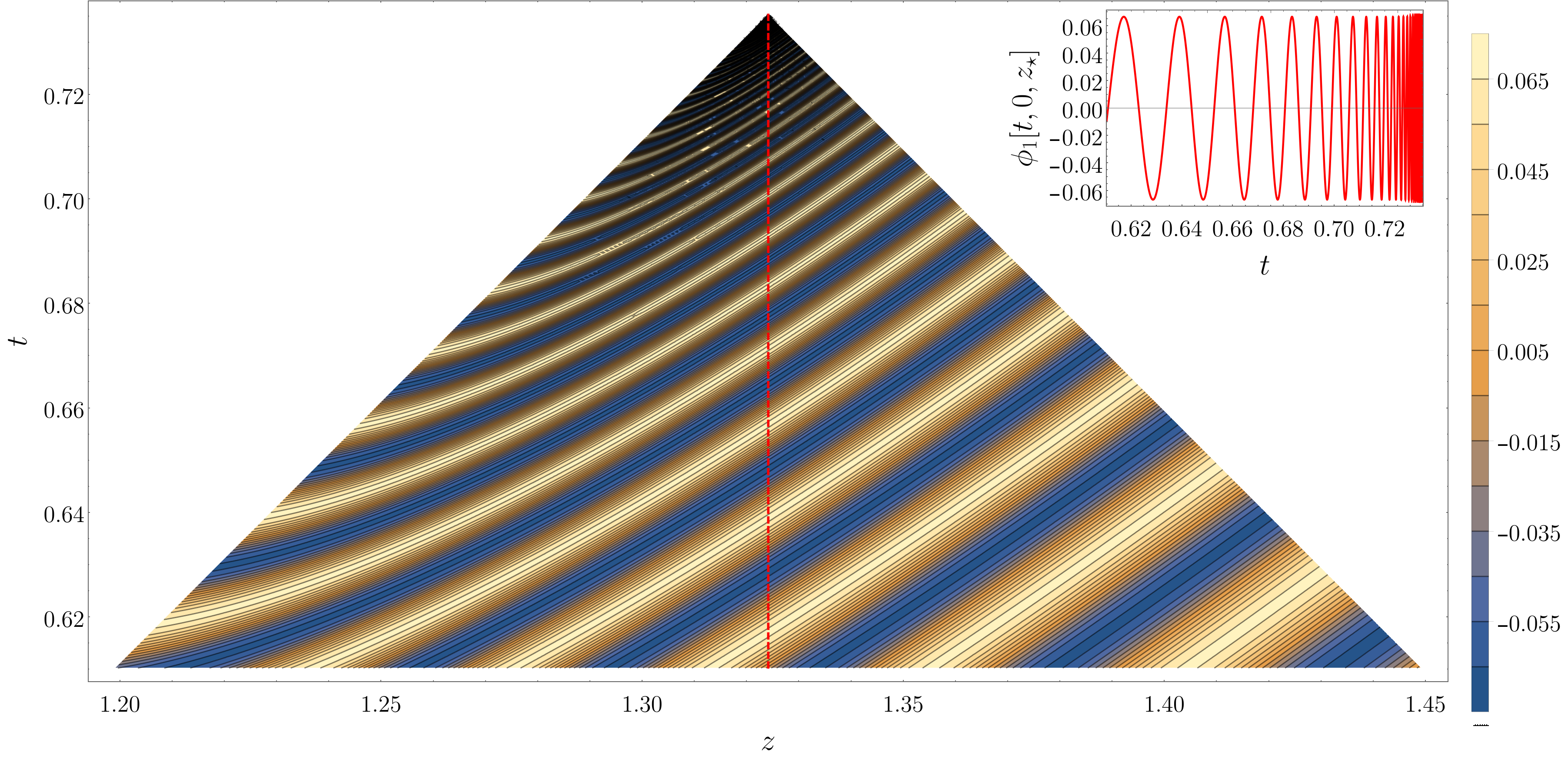
Figure 2: A contour plot of an axisymmetric threshold solution for model $3$ shown on the symmetry axis. Despite shared attributes with the spherical solution of Fig. 1, there are obvious differences too, as the data here leading to blow-up is mostly outgoing. For this model therefore the conjecture that there is in general a unique threshold solution regardless of initial data is false.

Regularity of spherical solutions at blow-up.

So far, we have focused only on pointwise blow-up, but a proper understanding of the threshold must also include statements about local integrability. Consider first deformation functions that involve only a compactification. As we have already discussed, with this setup blow-up solutions, whether generic or at the threshold, become unbounded pointwise. Therefore by Sobolev embedding $H^{2}$ must explode (see Eqn. (14)), but beneath that, the story is more subtle. By choosing initial data constant in space for the first time derivative out to some radius and then cutting off, it is clear that solutions can blow up in $L^{2}$ for any of our pure compactification deformation functions. But around the threshold, the solutions blow up in a special, localized manner, so that boundedness in $L^{2}$ depends on the specific deformation function / compactification. This must also fall-in line with the observations made in the previous section about regularity of self-similar functions. In fact, since the compactification determines also $\nu$, there must exist a relationship between the universal powers and regularity at the threshold. To examine this, we suppose that the integral is dominated by the values of the integrand at the origin. Expanding then, we find with the log compactification that

$$||\phi_{\star}||_{L^{2}} \sim e^{-3T/2}T\,, \quad||\phi_{\star}||_{E^{1}} \sim e^{-T/2}\,,$$

$$||\phi_{s}||_{L^{2}} \sim T\,, \quad||\phi_{s}||_{E^{1}} \sim e^{T}\,,$$ (62)

for threshold solutions. Here we used the fact that, at the threshold, the spatial scale on which the solution becomes large pointwise is fixed in the similarity coordinate $X$. We assumed that blow-up of the supercritical solution $\phi_{s}$ occurred at the origin with the spatial scale fixed in $r$, and set the slow-time $T=-\log(t_{\star}-t)$, with $t_{\star}$ the instant at which the solution explodes so that $T\to\infty$ at the blow-up. Thus this estimate on $\phi_{s}$ need not be verified in practice, and indeed it is easy to come up with examples in which $L^{2}(\phi_{s})$ is finite even at blow-up. For the alternative compactification (49) we find

$$||\phi_{\star}||_{L^{2}} \sim e^{(2n-3/2)T}\,, \quad||\phi_{\star}||_{E^{1}} \sim e^{(2n-1/2)T}\,,$$

$$||\phi_{s}||_{L^{2}} \sim e^{nT}\,, \quad||\phi_{s}||_{E^{1}} \sim e^{(n+1)T}\,.$$ (63)

Again these naive estimates on $\phi_{s}$ need not be satisfied, and serve only as an indication of possible behavior. All of these estimates can be verified numerically and are in agreement with the results in Section II. Moving on to deformation functions involving a periodic function, by construction, obviously solutions can never blow up in $L^{2}$. Proceeding as before, we have

$$||\phi_{\star}||_{E^{1}} \sim e^{-T/2}\,,\quad ||\phi_{s}||_{E^{1}}\sim e^{T}\,,$$ (64)

for model $3$ and

$$||\phi_{\star}||_{E^{1}} \sim e^{(2n-1/2)T}\,,\quad ||\phi_{s}||_{E^{1}}\sim e^{(n+1)T}\,,$$ (65)

with the composite deformation function $\sin\circ\,\mathcal{C}$ taking again the compactification (49). As mentioned in the discussion above, we have checked these predictions in practice by computing numerically norms for different blow-up solutions. Some examples are shown in Fig. 3. In summary, threshold solutions blow up at $t=t_{\star}$ in $H^{1}$ when $n\geq 1/4$ (that is $\nu\leq-1/2$), and in the CSS setting in $L^{2}$ when $n\geq 3/4$ ($\nu\leq-3/2$). The two take-aways are first, that generic blow-up solutions are less regular than threshold solutions, and second that there is a direct relationship between the universal power and the specific level of regularity.

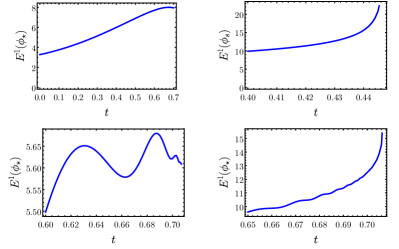
Figure 3: Plots of the $E^{1}$ norm for spherical solutions of various models up to the time at which some field quantity explodes in $L^{\infty}$. On the top left we have a threshold solution for model $1$. On the top right a supercritical solution for the same model is shown, demonstrating that a variation of behavior is possible at blow-up. On the bottom left we show the result for $\phi_{1}$ from model $3$ at the threshold. Finally in the lower right panel we show the same for the composite deformation function $\sin\circ\,\mathcal{C}$, with the compactification (49) and $n=1/4$, which can be used in practice within model $5$. These examples are compatible with our consideration of self-similar functions and our naive norm estimates.

Aspherical perturbations of spherical critical solutions.

So far we have established that in pure spherical symmetry threshold solutions of our deformation models depend to leading order on only one number from the initial data and are, in this sense, unique. Therefore, in accord with the usual picture of critical gravitational collapse, if we consider a one-parameter family of spherically symmetric initial data and tune this parameter to the threshold of blow-up we recover the critical solution. What is more, simply by continuous dependence on given data, spherical initial data close to the threshold generate solutions that appear like the critical solution for some time in their development. Evidently the latter statement is true also for nonspherical perturbations of the spherical critical solution. But in fact a stronger result holds. Take a family of spherical solutions $\phi_{a}(t,r)=D[a\,\varphi_{\star}(t,r)]$ normalized so that $a=1$ corresponds to the threshold solution $\phi_{\star}=\phi_{1}$. As discussed above, in the past light cone of the blow-up point, $\phi_{\star}$ is associated with a critical solution by simple Taylor expansion. Let $\tilde{\varphi}$ denote any regular partial wave solution (16) with vanishing spherical component $\tilde{\varphi}_{00}$. We may think of this solution as being parameterized by the infinite number of parameters stating how much of each of the individual partial wave solutions $\tilde{\varphi}_{lm}$, each of which also have a full functional degree of freedom, is present. Consider the perturbed solutions

$$\tilde{\phi}_{a}=D[a\,(\varphi_{\star}+\epsilon\,\tilde{\varphi})]\,,$$ (66)

and observe, crucially, from (18) that $\tilde{\varphi}_{lm}(t,r)=O(r^{l})$ near the origin. We then see that for $\epsilon$ sufficiently small $\tilde{\phi}_{\star}=\tilde{\phi}_{1}$ is also a threshold solution. Starting from $\tilde{\phi}_{\star}$, within this family the only way to restore global existence is to reduce the strength parameter $a$. It seems that this result would fit nicely with a perturbative analysis along the lines of that given in Martin-Garcia and Gundlach (1999). To understand the effect of the $\tilde{\varphi}$ on the asymptotic solution in the past light-cone of the blow-up point we present below a generalization of the spherical Taylor expansion given above.

Single-harmonic threshold solutions.

To this point the behavior exhibited by solutions of our models had a direct analog with the standard picture of critical collapse. In moving to consider general nonspherical threshold solutions we now part ways with that picture. The discussion here is focused on model $3$, but holds in fact more generally. We start by constructing a particular threshold solution from a pure $l=2$, $m=0$ partial wave solution $\varphi_{20}$ to the wave equation. Recalling the exact solution (18) and working with the family generated by the Gaussian,

$$F(r) =ae^{-(r+1)^{2}}\,,$$ (67)

we find that the threshold solution $\phi_{\star}$ is obtained with $a_{\star}\simeq 1.678$. As observed above, the partial wave vanishes at the origin, and therefore the blow-up point occurs elsewhere, in this case at $(t_{\star},x_{\star},y_{\star},z_{\star})\simeq(0.735,0,0,1.324)$. This threshold solution is plotted in Fig. 2. Although there clear are qualitative similarities with the spherical threshold solution plotted in Fig. 1 for the same model one could hardly claim that the two solutions are the same. Interestingly, even if we restrict to threshold solutions built from a single spherical harmonic in this manner there is still another distinct branch of threshold solutions. To see this consider, for example, the form of the $Y_{20}$ harmonic,

$$Y_{20} =\frac{1}{4}\sqrt{\frac{5}{\pi}}\big{(}3\cos^{2}\theta^{1}-1\big{)}\,,$$ (68)

which has local extrema on the $x$ and $z$-axes. Since we are concerned here with an axisymmetric solution we are free to identify $x$ with the cylindrical radial coordinate. Therefore our solution to the wave equation

$$\varphi =\varphi_{20}Y_{20}$$ (69)

giving rise to a solution of the deformed wave equation can explode the compactification in one of two ways,

$$\varphi_{20} =-2\sqrt{\frac{\pi}{5}}\,, \quad\varphi_{20} =4\sqrt{\frac{\pi}{5}}\,,$$ (70)

at some point, resulting in the first case in blow-up of $\phi$ on the symmetry axis as plotted in Fig. 2, or else on a ring in the $x\-y$-plane in the second. A snapshot of a solution close to this type of blow-up, obtained with the family

$$G(r) =-F(-r)\,,$$ (71)

with $F$ the Gaussian from before, is shown in Fig. 4.

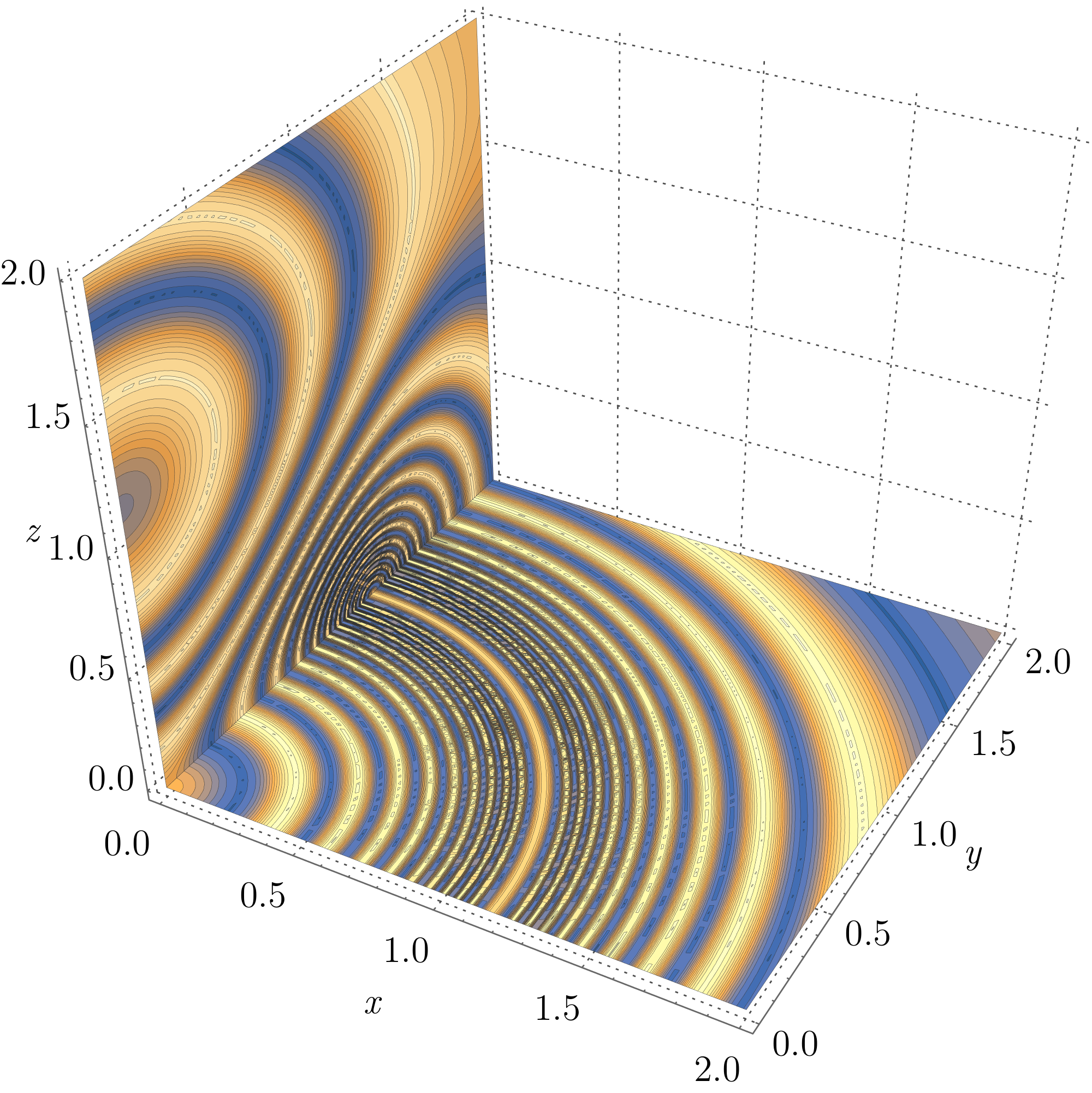
Figure 4: Here we plot a pure $l=2$, $m=0$ threshold solution for model $3$ shortly before blow-up. Special in this case is that the blow-up occurs on a ring in the $z=0$ plane. This was achieved with the family (71), which we may think of as the same data as (67), but evolved backwards in time. This shows that away from spherical symmetry, even when building threshold solutions purely from a single harmonic, there exist fundamentally different threshold solutions, although the number of such branches for each harmonic is always presumably finite. This story becomes even more involved with higher harmonics.

Blow-up amplitudes under perturbations.

The previous example shows that threshold solutions constructed from a generic single harmonic are not unique, and may differ even in the topology of their blow-up. In the spherical setting we have seen that adding arbitrary small perturbations to the initial data at the threshold nevertheless leave us with the same critical amplitude. So an obvious question is whether or not threshold solutions built from a single harmonic, or sum of harmonics are locally unaffected by adding additional harmonics in the same sense. The answer is no. To see this, recall that the mechanism for this outcome in the spherical case was that higher order partial wave solutions vanish at the origin, where blow-up is guaranteed to occur with spherical symmetry. In general the support of higher order partial waves includes however possible blow-up points induced by another partial wave solution. Therefore a small addition of a higher order partial wave can render a threshold solution small enough to avoid blow-up or drive it unambiguously over the threshold. The difference between the spherical and generic setup is illustrated by Fig. 5. General threshold solutions are thus described as a sum over all harmonics, with any individual harmonic potentially playing a role in the blow-up, and with different topologies, like the ring of Fig. 4, of the singular points possible. This behavior could be sidestepped if we re-expanded the solution in terms of translated spherical harmonics centered at the blow-up point, or more generally a point in the curve of blow-up points, to again recover a basis well-adapted to the solution at hand.

Self-similarity and generic threshold solutions.

By definition, a generic threshold solution can be obtained through the deformation $\phi_{\star}=D(\varphi_{\star})$, where $\varphi_{\star}$ is a solution of the flat-space wave equation such that for $t<t_{\star}$ we have $\varphi_{\star}(t,x^{i})>\xi_{\star}$, and $\varphi_{\star}(t_{\star},x^{i}_{\star})=\xi_{\star}$ is a local minimum. Again, the point $(t_{\star},x^{i}_{\star})$ is taken to be the location of blow-up of the deformed solution. Because $\varphi_{\star}$ is a local minimum at $(t_{\star},x^{i}_{\star})$, all first derivatives vanish at this point, and some second derivatives must be positive, like $\partial_{t}^{2}\varphi_{\star}$; however, the second derivatives $\partial_{t}\partial_{i}\varphi_{\star}$ and $\partial_{j}\partial_{i}\varphi_{\star}$ may be zero if the blow-up happens in a curve or a surface (as illustrated in Fig. 4). We assume here that the blow-up happens at a point, but the same discussion applies to any point in a curve or surface of blow-up, with the caveat that the past light cone of each such point can be treated locally as follows, with a global understanding to be tackled separately. Close to this blow-up point, the solution of the original flat-space wave equation is

$$\lim_{(t,x^{i})\to(t_{\star},x^{i}_{\star})}\varphi_{\star} \sim\xi_{\star}+\tfrac{1}{2}\partial_{t}^{2}\varphi_{\star}(t_{\star}-t)^{2}$$

$$-\partial_{t}\partial_{i}\varphi_{\star}(t_{\star}-t)(x^{i}-x^{i}_{\star})$$

$$+\tfrac{1}{2}\partial_{i}\partial_{j}\varphi_{\star}(x^{i}-x_{\star}^{i})(x^{j}-x^{j}_{\star})\,,$$ (72)

with all derivatives evaluated at $(t_{\star},x^{i}_{\star})$. Uniqueness of the threshold solution in the spherical case, and the lack thereof in general, can be understood here from the fact that the derivatives in the former case depend only on the $l=m=0$ partial wave solution, whereas in general higher harmonics can contribute. To count the number of free-parameters here, first observe that, performing a trace-trace-free decomposition on $\partial_{i}\partial_{j}\varphi_{\star}$, the Laplace piece can be replaced using the wave equation. We then count nine free parameters. If we introduce a spherical harmonic decomposition of $\varphi_{\star}$ centered at $x_{\star}^{i}$, it follows by the $O(r^{l})$ property of the partial waves that only the lowest order (up to $l=2$) harmonics can contribute, which gives a consistent count of parameters. The first derivatives are

$$\lim_{(t,x^{i})\to(t_{\star},x^{i}_{\star})}\partial_{t}\varphi_{\star} \sim\partial_{t}^{2}\varphi_{\star}(t_{\star}-t)+\partial_{t}\partial_{i}\varphi_{\star}(x^{i}-x^{i}_{\star})\,,$$

$$\lim_{(t,x^{i})\to(t_{\star},x^{i}_{\star})}\partial_{i}\varphi_{\star} \sim\partial_{i}^{2}\varphi_{\star}(t_{\star}-t)-\partial_{t}\partial_{i}\varphi_{\star}(t_{\star}-t)\,.$$ (73)

Let’s look at the models arising from deformations using periodic functions. Using model $3$, for instance, which has $\xi_{\star}=-1$, we have

$$\lim_{(t,x^{i})\to(t_{\star},x^{i}_{\star})}\partial_{t}\phi_{1\star}\sim$$

$$\quad-\lim_{(t,x^{i})\to(t_{\star},x^{i}_{\star})}\cos\left[A_{3}^{-1}\log\left(1+\varphi_{\star}\right)\right]\frac{\partial_{t}\varphi_{\star}}{1+\varphi_{\star}}$$ (74)

and

$$\lim_{(t,x^{i})\to(t_{\star},x^{i}_{\star})}\partial_{i}\phi_{1\star}\sim$$

$$\quad-\lim_{(t,x^{i})\to(t_{\star},x^{i}_{\star})}\cos\left[A_{3}^{-1}\log\left(1+\varphi_{\star}\right)\right]\frac{\partial_{i}\varphi_{\star}}{1+\varphi_{\star}}\,.$$ (75)

Close to the point $(t_{\star},x^{i}_{\star})$, the denominator $(1+\varphi_{\star})$ is quadratic in $(t_{\star}-t,x^{i}-x_{\star}^{i})$ and the first derivatives $\partial_{t}\varphi_{1\star}$ and $\partial_{i}\varphi_{1\star}$ are linear in the same argument. So, the argument applied to spherically symmetric solutions goes through, and we conclude that the blow-up of $\partial_{t}\phi_{1\star}$ and $\partial_{i}\phi_{1\star}$ is DSS, centered at $(t_{\star},x^{i}_{\star})$, with $\nu=-1$ and $\lambda_{m}=e^{-m\Delta}=e^{m\pi A_{3}}$. Thus we find that the CSS and DSS blow-up properties of spherically symmetric threshold solutions, and even the non-standard behavior with our more general compactifications like in model $5$, can be extended to arbitrary threshold solutions. Now, however, nine parameters rather than one are required to characterize the asymptotic solution in the past-light cone of the blow-up point.

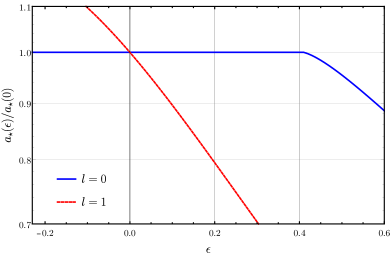
Figure 5: Plots of the blow-up threshold amplitude starting from either a pure spherical solution (blue curve) or an $l=1,m=0$ solution (red dashed curve), and adding in each case by $l=2,m=0$ spherical harmonic parameterized by $\epsilon$. See the main text following Eqn. (66) for details. There is a neighborhood around the spherical solution in which the nonspherical deformation makes absolutely no difference to critical amplitude, although the asymptotic solution in the past light cone of the blow-up point is modified. Once the perturbation is sufficiently large however the blue curve does bend away. At this point the threshold solution takes a structure similar to that illustrated in Fig. 2. We expect that when the blue curve is extended to the left, eventually the threshold solution will take the form illustrated in 4. In contrast, the pure $l=1$ threshold amplitude is immediately affected by the perturbation.

Power-law scaling around general threshold solutions.

So far we have discussed power-law behavior that occurs in physical space. In critical collapse such behavior is usually viewed in phase-space. We turn our attention to this next, working with the time derivative of the field, since this allows us to treat both types of model in a unified way. Consider a family of solutions $\phi_{a}=D[a\,\varphi]$, parameterized by $a$, with $\varphi$ a fixed, nontrivial solution of the wave equation which explodes the deformation function first at $a=a_{\star}$ as usual. Let $x^{\mu}(a)$ be the locus of maxima (in amplitude) of $\Pi_{a}=\partial_{t}\phi_{a}$, which we assume defines a curve when $a\lesssim a_{\star}$, with $a_{\star}$ the threshold amplitude. Since $\Pi_{a}$ attains a local maxima at $x^{\mu}(a)$, we have

$$\partial_{t}\Pi_{a}=aD^{\prime}(a\,\varphi)\partial_{t}^{2}\varphi+a^{2}D^{\prime\prime}(a\,\varphi)(\partial_{t}\varphi)^{2}=0\,,$$ (76)

which is understood to hold at $x^{\mu}(a)$, and which we can solve for $(\partial_{t}\varphi)^{2}$. Since this equation must hold for all values of $a$, we can derive in $a$, and obtain an expression for $t^{\prime}(a)$ in terms of the other variables. Assuming more regularity on the curve, we are free to take higher derivatives too. Starting with the general expression for $\Pi_{a}$ we then get

$$\Pi_{a}(x^{\mu}(a))^{-2} =\frac{D^{\prime\prime}(a\,\varphi)}{aD^{\prime}(a\,\varphi)^{3}\partial_{t}^{2}\varphi}\,,$$ (77)

again understood to hold at $x^{\mu}(a)$. From here we split our discussion into two cases. First suppose that $D=\mathcal{C}$ with our compatification (49), assuming that $n>0$. In this case (77) takes the form,

$$\Pi_{a}(x^{\mu}(a))^{-2} =-\frac{\mathcal{C}^{\prime\prime}(a\,\varphi)}{a\mathcal{C}^{\prime}(a\,\varphi)^{3}\partial_{t}^{2}\varphi}=\frac{(1+a\,\varphi)^{2n+1}}{a\,\partial_{t}^{2}\varphi}\,.$$ (78)

We need to extract the piece of this that dominates as $a\to a_{\star}$. Since $\partial_{t}^{2}\varphi$ is generically non-zero at the maximum and non-zero as $a\to a_{\star}$, we need only consider

$$\frac{\mathcal{C}^{\prime\prime}(a\,\varphi)}{\,\mathcal{C}^{\prime}(a\,\varphi)^{3}} =-(n+1)(1+a\,\varphi)^{2n+1}\,.$$ (79)

Raising this to the power $1/(2n+1)$, Taylor expanding at an arbitrary $a=a_{0}$, plugging in the result for $t^{\prime}(a)$, and taking the limit $a_{0}\to a_{\star}$ we conclude that, in the regime $a\lesssim a_{\star}$, we have

$$\Pi_{a}(x^{\mu}(a)) \simeq(a-a_{\star})^{-(2n+1)/2}\,.$$ (80)

The logarithmic compactification used in (21) is more subtle to treat, but corresponds to the case $n=0$. In fact for this model the range $-1/2<n<0$ may also be interesting to investigate, but we do not do so here. Moving now to the case $D=\mathcal{P}\circ\mathcal{C}$, again for concreteness taking the compactification from (49), we find that (78) is instead replaced by

$$-\Pi_{a}(x^{\mu}(a))^{-2} =\frac{\mathcal{P}^{\prime\prime}}{a\mathcal{P}^{\prime 3}\mathcal{C}(a\,\varphi)\partial^{2}_{t}\varphi}+\frac{\mathcal{P}^{\prime}\mathcal{C}^{\prime\prime}(a\,\varphi)}{a\mathcal{P}^{\prime 3}\mathcal{C}(a\,\varphi)^{3}\partial^{2}_{t}\varphi}\,.$$ (81)

Following from here the same procedure as before, noting that the first of these terms is now the leading piece, and raising to the power $1/(n+1)$, in the regime $a\lesssim a_{\star}$, we find that

$$\Pi_{a}(x^{\mu}(a)) \simeq(a-a_{\star})^{-(n+1)/2}\,.$$ (82)

Again the $\log$ compactification can be thought of as $n=0$. With a little more care we expect that one could see here also the superposed periodic wiggle. An important message here is that power-law behavior may appear even in models for which self-similarity is absent at the threshold, so evidence of both phenomena are needed for a confident diagnosis. In summary, we find that under mild assumptions on the regularity of $x^{\mu}(a)$, close to the threshold, all of our models admit universal power-laws regardless of the nature of the threshold solution itself. Nevertheless some care is needed in interpreting this result. For general data there may appear multiple “large-data” regions, and the peak of that which ultimately leads to blow-up in the limit $a\to a_{\star}$ may be obfuscated, over some range of $a$, by another.

Regularity of threshold vs. generic blow-up solutions.

Recovering results on the norms of threshold and blow-up solutions in the nonspherical setting is trickier than the previous case. Although the only numerical part of the calculation is in the evaluation of the norm itself, the solutions can be highly oscillatory. Nevertheless in all of the cases that we can reliably verify, which include all of those presented in Fig. 3, we find that our spherical results carry over without any surprises, and that threshold solutions are slightly more regular than generic blow-up solutions. In the future it will be interesting to use the geometric reformulation of our models given in Sec. III together with the conserved stress-energy to prove these properties beyond doubt.

V Numerical Results

In the previous section we gave a fairly complete picture of threshold solutions for the models that arise as a deformation of the wave equation. To address the obvious criticism that such models may not be qualitatively representative of systems that do not arise as a deformation, we now present numerical evidence that similar phenomenology does occur within our non-deformation models. Presently we restrict to spherical symmetry, postponing detailed numerical of generic threshold solutions for future work. We begin by explaining briefly the method used, before presenting the classification and numerical results for each model. Similar, though more comprehensive, numerical work for alternative models can be found in Liebling (2002); Bizon et al. (2004); Liebling (2005); Bizoń et al. (2007); Bizon and Zenginoglu (2009).

V.1 Methods

As presented in section III, all model equations are second order both in time and space. For the code we reduce the system to fully first order form and use centered finite differences. To do so we introduce the following auxiliary evolved fields,

$$\Phi=\partial_{r}\phi\,,\qquad\qquad\Pi=\partial_{t}\phi\,.$$ (83)

In order to deal with the coordinate singularity at the origin, we apply the Evans method, for any scalar field $\Psi$ and its derivative $\Psi^{\prime}=\frac{d\Psi}{dr}$, with $p=2$ Evans (1984),

$$\Psi^{\prime}+\tfrac{p}{r}\Psi=(p+1)\frac{d(r^{p}\Psi)}{d(r^{p+1})}\,,$$ (84)

where the differential operator can be expressed in terms of the grid points as,

$$(p+1)\frac{d(r^{p}\Psi)}{d(r^{p+1})}=(\tilde{D}\Psi)_{i}=(p+1)\frac{r^{p}_{i+1}\Psi_{i+1}-r^{p}_{i-1}\Psi_{i-1}}{r^{p+1}_{i+1}-r^{p+1}_{i-1}}.$$ (85)

In section II definitions for the different norms we consider were given, and their blow-up for CSS and DSS functions was introduced and related. Below in this section we classify the models presented in section III following this criteria. We employ the method of lines with a Runge-Kutta $4$ time integrator, and to avoid rapid growth of numerical error we use second order Kreiss-Oliger artificial dissipation Kreiss and Oliger (1973) with a small dissipation parameter of order $\sigma=0.02$. The particular boundary conditions for each model are stated at their corresponding section.

V.2 CSS and $L^{\infty}$ blow-up

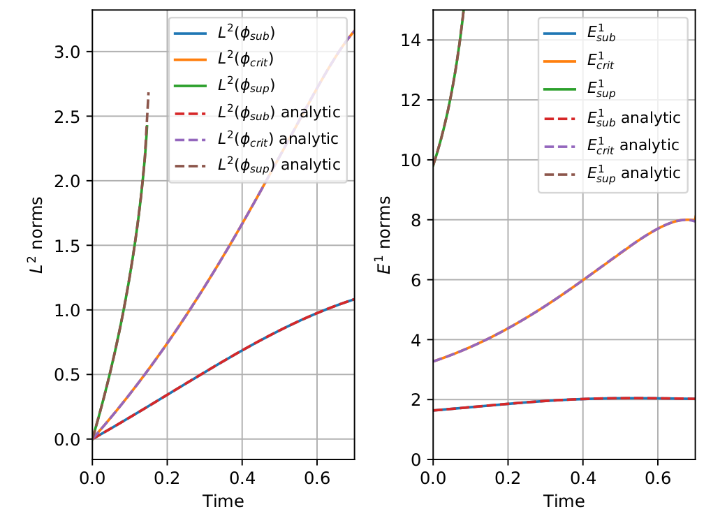
Figure 6: $L^{2}$ and $E^{1}$ for model $1$ for sub, critical and supercricital data computed from our numerical simulations and the exact solution for model $1$ with $A_{1}=-1$. The numerical data agree extremely well with the values computed from the exact solution. This indicates that, with suitable care, numerical evolutions can be of real value in determining regularity even at blow-up.

Model $\bm{1}$.

The equations of motion for the auxiliary fields are,

$$\partial_{t}\Phi =\partial_{r}\Pi\,,$$

$$\partial_{t}\Pi =\partial_{r}\Phi+\tfrac{2}{r}\Phi+A_{1}\left(\Phi^{2}-\Pi^{2}\right).$$ (86)

We impose the condition

$$\partial_{t}\Pi\;\hat{=}-\partial_{r}\Pi,$$ (87)

at the outer boundary. Modulo boundary effects which are negligible in our present study, we can write down closed form solutions for this model, so numerical work constitutes only a code-test. But such work can be highly valuable as it may give confidence in purely numerical studies and highlight algorithmic shortcomings. We have performed numerical evolutions with a variety of initial data and find that the method converges reliably at second order as expected. As observed in section IV this model is an example with approximately CSS threshold behavior. All blow-up solutions, including those at the threshold, explode in $L^{\infty}$, but nevertheless may remain finite and even in $L^{2}$ and even in the energy norm $E^{1}$. At the threshold solutions are finite in $E^{1}$, whereas generically blow-up solutions explode in $E^{1}$. An important question therefore is how well numerical methods can cope with data at these varying levels of regularity. Pessimistically one might expect that with standard methods when the solution explodes pointwise, numerical error becomes large so fast that any approximation to $L^{2}$ (and so forth) from the numerical data also diverges. We have investigated this, as shown for example in Fig. 6, and find that the numerics capture the expected behavior well. In the future it may be useful to examine the same question for models that have different regularity at blow-up, for example by using our parameterized compactification (49).

Model $\bm{2}$.

The equations of motion for the reduction variables are

$$\partial_{t}\Phi_{1} =\partial_{r}\Pi_{1}\,,\qquad\partial_{t}\Phi_{2}=\partial_{r}\Pi_{2}\,,$$

$$\partial_{t}\Pi_{1} =\partial_{r}\Phi_{1}+\tfrac{2}{r}\Phi_{1}+A_{2}\left(\Pi_{2}^{2}-\Phi_{2}^{2}\right)\,,$$

$$\partial_{t}\Pi_{2} =\partial_{r}\Phi_{2}+\tfrac{2}{r}\Phi_{2}+B_{2}\left(\Pi_{1}^{2}-\Phi_{1}^{2}\right)\,.$$ (88)

At the outer boundary we impose

$$\partial_{t}\Pi_{1}\;\hat{=}-\partial_{r}\Pi_{1}\,,\qquad\partial_{t}\Pi_{2}\;\hat{=}-\partial_{r}\Pi_{2}\,.$$ (89)

We have evolved and tuned to the threshold of blow-up with several families of initial data, but here discuss a representative example with initial data,

$$\Phi_{1}(0,r) =\Phi_{2}(0,r)=0\,,$$

$$\Pi_{1}(0,r) =\tfrac{2}{5}e^{1/2-r^{2}}\,,\quad\Pi_{2}(0,r)=ae^{1/2-r^{2}}\,.$$ (90)

We have experimented with various choices for the parameters $A_{2}$ and $B_{2}$, which do not seem to affect the qualitative behavior of solutions. Recall that if we choose $A_{2}=B_{2}=A_{1}$ and set $\phi_{1}=\phi_{2}$ we recover solutions of model $1$, making this choice of the parameters an interesting point to investigate in more detail. In Fig. 7 we do so by plotting the logarithm of the maximum of the time derivative of the scalar field at the origin ($\Pi_{1}(t,0)_{\textrm{max}}$, $\Pi_{2}(t,0)_{\textrm{max}}$) against the logarithmic distance to the critical point $a_{\star}$ together with their respective linear least-squares regressions. Note that hereafter $a$ is the only parameter in each family of solutions and $a_{\star}$ refers to its critical value in each case. Note that there are two lines, one red and one green, but near the threshold they perfectly overlap and give, as a result, the figures mentioned above. Interestingly, in fact we find that for any strong data, with $A_{2}=B_{2}$, the two sets $(\phi_{1},\Phi_{1},\Pi_{1})$ and $(\phi_{2},\Phi_{2},\Pi_{2})$ miraculously coincide, and so in fact threshold solutions agree with those of model $1$. This behavior is shown in the right panel of Fig. 7. Scaling shows that if $A_{2}B_{2}>0$ then,

$$A_{1}^{-1}(A_{2}B_{2}^{2})^{1/3}\phi_{1}\,,\qquad A_{1}^{-1}(A_{2}^{2}B_{2})^{1/3}\phi_{2}\,,$$ (91)

solve the same model with fresh constants $A_{2}^{\prime}=B_{2}^{\prime}=A_{1}$. This is of course borne out in our simulations. Our numerical evidence therefore strongly suggests that all spherical threshold solutions can be constructed directly from model $1$. We conclude that model $2$ does indeed have a unique critical solution in spherical symmetry. Given this, it is perhaps not surprising that experiments indicate the same level of regularity in $L^{2}$ and $E^{1}$ for this model as for model $1$ in Fig. 6 for subcritical, critical and supercritical initial data.

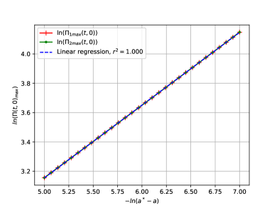
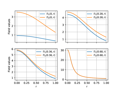
Figure 7: In the left panel we plot the scaling law obtained close to the threshold by taking the maximum of the time derivatives of the evolved fields $\phi_{1},\phi_{2}$ for Model $2$. We have chosen $A_{2}=B_{2}=-1$, and used initial data as stated in (90). The threshold amplitude $a_{\star}=1.5103468$ was obtained by numerical bisection. In the legend $r^{2}$ refers to the square of the Pearson correlation coefficient, which we computed using the Scipy Python library Virtanen et al. (2020). A best fit on the data at this resolution returns the gradient $0.49594$ with standard error $0.00018$. On the right we plot snapshots of the same fields close to blow-up for the threshold solution itself. Observe that the fields lie on top of each other in the at late times, indicating that the threshold solution is in fact described by the same critical solution of model $1$. Identical results are obtained with other families of initial data.

V.3 DSS models and their blow-up

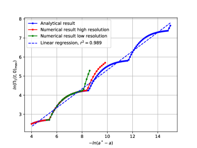
Figure 8: Scaling plot for $\Pi_{1}(t,0)_{\textrm{max}}$ for model $3$ with $A_{3}=1$ for the family of initial data (94). The threshold amplitude for this family is $a_{\star}=-\sqrt{2}$. For comparison the analytic result is also given. The drift between the numerical and analytic curves is caused by numerical error, but does converge away with resolution, as can be understood from the higher resolution data. In the legend $r^{2}$ again refers to the square of Pearson correlation coefficient, which was computed from the lower resolution data and is close to unity. Linear regression on the numerical data gives the gradient $0.4945$, with standard error $0.0049$, close to the expected value $1/2$ seen in Sec. IV.

Model $\bm{3}$.

The equations of motion for the third model,

$$\partial_{t}\phi_{1} =\Pi_{1}\,,\quad\quad\partial_{t}\phi_{2}=\Pi_{2}\,,$$

$$\partial_{t}\Phi_{1} =\partial_{r}\Pi_{1}\,,\quad\partial_{t}\Phi_{2}=\partial_{r}\Pi_{2}\,,$$

$$\partial_{t}\Pi_{1} =\partial_{r}\Phi_{1}+\tfrac{2}{r}\Phi_{1}$$

$$\quad+A_{3}^{-2}(\phi_{1}+A_{3}\phi_{2})[\Phi_{1}^{2}+\Phi_{2}^{2}-\Pi_{1}^{2}-\Pi_{2}^{2}]\,,$$

$$\partial_{t}\Pi_{2} =\partial_{r}\Phi_{2}+\tfrac{2}{r}\Phi_{2}$$

$$\quad+A_{3}^{-2}(\phi_{2}-A_{3}\phi_{1})[\Phi_{1}^{2}+\Phi_{2}^{2}-\Pi_{1}^{2}-\Pi_{2}^{2}]\,,$$ (92)

are supplemented with the corresponding boundary conditions,

$$\partial_{t}\Pi_{1}\;\hat{=}-\partial_{r}\Pi_{1}-\tfrac{1}{r}\Pi_{1}\,,\quad\partial_{t}\Pi_{2}\;\hat{=}-\partial_{r}\Pi_{2}-\tfrac{1}{r}\Pi_{2}\,.$$ (93)

These boundary conditions are modified with respect to those of the previous models simply to avoid code crashes, but in all applications we nevertheless keep the outer boundary causally disconnected from the region at the center we are actually interested in. Like model $1$, we know form solutions here, and so view these numerics primarily as a code-test. In this spirit, in Fig. 8 we again show the logarithm of the maximum of the time derivative $\Pi_{1}(t,0)_{\textrm{max}}$ against the logarithmic distance to the critical point for a representative family of initial data given by

$$\phi_{1}(0,r) =0\,, \quad\phi_{2}(0,r)=1\,,$$

$$\Phi_{1}(0,r) =0\,, \quad\Phi_{2}(0,r)=0\,,$$

$$\Pi_{1}(0,r) =ae^{1/2-r^{2}}\,, \quad\Pi_{2}(0,r)=0\,,$$ (94)

in this instance using $A_{3}=1$. In all cases we clearly observe the expected DSS behavior, which manifests as a straight line plus a periodic wiggle whose period depends on the value of $A_{3}$. Regarding regularity, recall that this model actually has the similar behavior as model $1$. Although the solution itself never diverges, first derivatives are divergent for any blow-up solution. Solutions are always finite in $L^{2}$. At the threshold $E^{1}$ is finite, but for all other blow-up solutions it diverges. We have examined how well this behavior is captured in our numerical approximation and find that results similar to those displayed in Fig. 6 are easily obtained, albeit with $L^{2}$ finite, and that these results agree very well with those computed directly from the exact solution, even at blow-up.

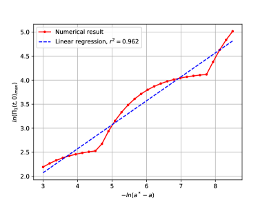
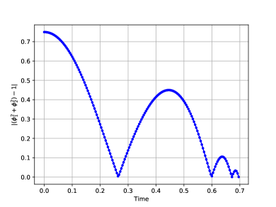
Figure 9: Representative plots obtained with model $4$ with $A_{4}=B_{4}=1$ and the initial data family (96). This is obtained with $a_{\star}\simeq-2.4122$. On the left we give the now familiar scaling plot for $\Pi_{1}$. As in model $3$ the curve looks like a straight line plus a periodic wiggle, indicating that we are in a DSS regime. Linear regression on the numerical data gives a slope $0.499$, with standard error $0.019$. On the right we plot the maximum of the absolute value at the origin of the quantity that serves as a constraint in model $3$. In fact this quantity is small in a neighborhood around the origin, so that near the threshold, solution of model $4$ are close to solutions of model $3$.

Model $\bm{4}$.

The final model that we implemented is an extension of model $3$ in which the constraint $\phi_{1}^{2}+\phi_{2}^{2}=A_{3}$ is violated. The equations of motion in the case are,

$$\partial_{t}\phi_{1} =\Pi_{1}\,,\quad\quad\partial_{t}\phi_{2}=\Pi_{2}\,,$$

$$\partial_{t}\Phi_{1} =\partial_{r}\Pi_{1}\,,\quad\partial_{t}\Phi_{2}=\partial_{r}\Pi_{2}\,,$$

$$\partial_{t}\Pi_{1} =\partial_{r}\Phi_{1}+\tfrac{2}{r}\Phi_{1}$$

$$\quad+A_{4}^{-2}(\phi_{1}+A_{4}\phi_{2})[\Phi_{1}^{2}+\Phi_{2}^{2}-\Pi_{1}^{2}-\Pi_{2}^{2}]\,,$$

$$\partial_{t}\Pi_{2} =\partial_{r}\Phi_{2}+\tfrac{2}{r}\Phi_{2}$$

$$\quad+B_{4}^{-2}(\phi_{2}-B_{4}\phi_{1})[\Phi_{1}^{2}+\Phi_{2}^{2}-\Pi_{1}^{2}-\Pi_{2}^{2}]\,.$$ (95)

In this case, the two scalar fields of the model are not, a priori, related to each other because solutions do not arise from a deformation of the wave equation. In Fig. 9 we plot the logarithm of the maximum of the time derivative $\Pi_{1}(t,0)_{\textrm{max}}$ against the logarithmic distance to the critical point and observe that this model, despite violating the constraint and not coming from a deformation of the wave equation, exhibits DSS behavior too. In this particular plot we worked with $A_{4}=B_{4}=1$, and the family of initial data,

$$\phi_{1}(0,r) =0\,, \quad\phi_{2}(0,r)=\tfrac{1}{2}\,,$$

$$\Phi_{1}(0,r) =0\,, \quad\Phi_{2}(0,r)=0\,,$$

$$\Pi_{1}(0,r) =ae^{1/2-r^{2}}, \quad\Pi_{2}(0,r)=0\,.$$ (96)

and tuned to the threshold $a_{\star}=-2.4122175$ by numerical bisection. Similar to model $2$, close to the threshold we observe that, at least for the families of data that we tested, the “constraint” is in fact small close to criticality. We observe similar behavior for any blow-up solution, but it is most pronounced at the threshold. This is illustrated in the second plot of Fig. 9. We do note however, that this behavior is not as striking as in model $2$, where the “constraint” seems identically satisfied over an entire region, rather than just being small as in this case. Concerning regularity, at the threshold the raw fields $\phi_{1}$ and $\phi_{2}$ remain finite (and thus the solution remains finite in $L^{2}$), but as shown in the discussion above first derivatives do explode. Our data suggest that the energy norm $E^{1}$ is finite at the threshold but diverges for supercritical solutions, in agreement with model $3$. Having examined several different families of initial data, our numerical evidence again suggests that in spherical symmetry model $4$ has a unique critical solution in the same sense as our other models.

VI Conclusions

The cosmic censorship conjectures are perhaps the most important open problems in strong-field gravity. In looking for evidence either for or against them it is imperative that we examine extreme regions of the solution space. Combining such considerations with numerical approximation, critical phenomena in gravitational collapse have been discovered. The standard picture of critical collapse is that, if we consider any one-parameter family of initial data and tune that parameter to the threshold of black hole formation, then as it heads towards blow-up the resulting threshold solution will approximate ever more closely, in the strong-field region, a unique self-similar critical solution which has a naked singularity. In suitable coordinates data within the family, but close to the threshold, approach the critical solution for some time interval $\sim-\gamma^{-1}\log|a-a_{\star}|$ before either dispersing or collapsing, with $\gamma$ a universal parameter independent of the particular family. Examining solutions parametrically in a neighborhood of the threshold reveals that the curvature scalars, black hole masses and so forth display power-law behavior, with power $\gamma$, in $a_{\star}-a$.

In spherical symmetry numerical evidence in favor of this picture is pristine, and there is even a proof Reiterer and Trubowitz (2019) that the Choptuik critical solution, with the posited discrete self-similarity, exists. Part of this phenomenology remains robustly without symmetry, but cracks have appeared in the picture. Prominent examples are given by the variability of the scaling parameters and apparent contradiction of uniqueness of the critical solution in scalar field collapse when large aspherical perturbations are present Choptuik et al. (2003); Baumgarte (2018), the seeming absence of a unique self-similar critical solution in the collapse of the electromagnetic fields Baumgarte et al. (2019) and the consistent challenge in treating threshold solutions in vacuum gravity Hilditch et al. (2013, 2016, 2017) and so in recovering the results of Abrahams and Evans (1993). In all of these cases however, we are reaching to the edge of what is possible with present numerical methods, so there are arguments against adjusting the standard picture until numerical error could be reliably controlled.

In the present study we therefore sought a way to side-step these difficulties by constructing the absolute simplest school-boy model that could capture the qualitative behavior of interest. Our models are based on a trick of Nirenberg, admit a small-data global existence result, and in most cases be solved analytically, making interpretation of threshold solutions unambiguous, regardless of symmetry. We call these deformation models. In contrast with earlier models, they also have the advantage, at least from the point of view of gravitation, that their nonlinearity appears in first derivatives of the fields, just as in GR nonlinearities are of the form “$\Gamma^{2}-\Gamma^{2}$”. To the best of our knowledge we have also given the first such model that admits discretely self-similar solutions. (Other examples with such solutions are known Tao (2016) but require a large number of fields). Although the models can be reformulated in a natural way that introduces a non-trivial spacetime metric, they are nevertheless fundamentally tied to the flat-metric, and so should not be thought of as a model for weak cosmic censorship. Rather, at best we can hope to capture the properties required for strong cosmic censorship in terms of regularity at blow-up and of course those of critical collapse. Our findings, conclusions and conjectures can be split into categories discussed in turn in the next paragraphs.

Spherical symmetry.

Restricting to pure spherical symmetry, the obvious analog of the standard picture of critical collapse was completely vindicated for all of our models regardless of how they arose. For our deformation models, simple Taylor expansion shows that generically at most one number from the initial data survives to parameterize the threshold solution near the blow-up point. In fact there is a measure-$0$ special case in which this parameter vanishes, but we have not investigated this in detail. We define this one-parameter family of Taylor expanded threshold solutions to be the critical solution. In that one parameter remains, it is unique in the same sense the Schwarzschild is the unique static vacuum solution. Extracting this parameter in any numerical setup seems impractical, however. For models that do not arise as a deformation of the wave equation, we tackled the spherical setting numerically and found evidence compatible with this picture. With either type of model we found that universal power-law behavior, for example in the maximum of any divergent field quantity, like for example energy density, was manifest. This was shown analytically for the deformation models. Moving on to consider small aspherical perturbations, to avoid having to perform more costly numerics we studied only deformation models. We found that the critical amplitude remains fixed, and that the blow-up itself is still dominated by the lowest spherical harmonic. From a purely mechanical point of view, this is a simple consequence of the fact that aspherical partial wave solutions all vanish at the origin. Nevertheless the asymptotic threshold solution, which maintains the scale-symmetry from the spherical setting, is deformed as perturbations are added, perhaps in contradiction expectations, so that a larger number of parameters are needed for its description. Power-law scaling in this regime, both in the physical and phase space pictures, also remains universal. The agreement with the standard picture of critical collapse in the regime in which numerical results are unambiguous, is striking. This gives us confidence that our models do capture qualitatively the phenomena of interest, and potentially do have predictive power for GR.

Strong cosmic censorship.

As mentioned in the introduction, the strong cosmic censorship conjecture may be thought of as the requirement that for generic initial data the resulting solution, when maximally extended, is unique. In the context of blow-up, typically in the context of black hole interiors as in Poisson and Israel (1990); Cardoso et al. (2018), this is taken to mean that at a Cauchy horizon, or more generally in the limit towards any the end-point of any incomplete geodesic, the metric should lose enough regularity that the solution can not be extended beyond the blow-up, even if we allow weak solutions. If this fails to be the case, perhaps by choosing fresh data at the singular surface, we may obtain many inequivalent extensions and so violate global uniqueness. The specific requirement in GR Christodoulou (1999) is that there exist no coordinates in which the Christoffel symbols are locally $L^{2}$. The natural analog for our models is the requirement that, at blow-up, solutions explode in the energy norm $E^{1}$. The conclusion from our models is that for each type of model there exists a direct, specific, relationship between the physical and phase space power-law parameters $\nu$ and $\gamma$, and the regularity of data at blow-up. We find that threshold solutions are more regular than generic blow-up solutions, and so depending on the values of these parameters solutions could be extended beyond the blow-up point. We have not investigated this in detail, and this result may have no direct counterpart in GR, but if it does it will permit numerical simulations a new say on strong cosmic censorship in a variety of scenarios.

The threshold of blow-up.

When considering either large aspherical deformations of spherical threshold solutions or general threshold solutions we depart from the standard picture of critical collapse. But from an empirical point of view, our results in this regime are nevertheless compatible with numerical results in GR. First, power-law scaling persists both in physical space near the blow-up point, and also in phase space as the threshold is approached. In GR there is evidence, in scalar field collapse, that power-law rates deviate from their values in spherical symmetry as large asphericity appears Choptuik et al. (2003); Baumgarte (2018) so this is a possible difference to the models. That said, it is not obvious that the available numerical data are sufficiently fine-tuned to recover the limiting rates, and the interactions of multiple fields complicate the interpretation. If spherical data for the models are perturbed by a sufficiently large asphericity, blow-up occurs away from the origin, with the solution displaying appearing very different to the spherical critical solution in the past light cone of the blow-up point, in contradiction with the expectation that there exist a unique critical solution in the general setting. This may manifest, for example by the formation of multiple nonspherical centers away from the origin. The latter has been observed in GR in both scalar field Choptuik et al. (2003); Baumgarte (2018) and vacuum collapse Hilditch et al. (2017). As illustrated in Fig. 4 blow-up can even occur on curves rather than points, an important possibility to be investigated in the gravitational context. Depending on the model, general threshold solutions may exhibit self-similarity, but require several parameters to describe them as they approach blow-up. In GR, by analogy, the existence of a single critical solution would be a red-herring in general. Instead, the threshold of collapse should be characterized by power-law scaling, and, crucially, additional regularity with respect to general blow-up solutions. Recalling that we have models which display these features, but do not satisfy the formal definition of self-similarity at the threshold, and the lack of exact self-similarity in nonspherical numerical work for GR, we conjecture that in the past light cone of a blow-up point, threshold solutions in GR can still be described by a finite number of parameters. In this way, we can still use the language critical solution, but that solution must now be thought of as a parameterized family, whose specific nature is, for now, uncertain.

Future work.

The study of model problems can never definitively solve problems in the full generality that we would wish. Several possibilities present themselves for future developments. Regarding our models, it is highly desirable to develop tools to rigorously prove, without using the exact solutions, the properties of the solutions we have uncovered, and to satisfactorily explain what are the structural conditions that determine either CSS or DSS behavior at the threshold. Obvious directions for numerical work are to compute threshold solutions to the models without symmetry, and to examine carefully whether or not the solution space of GR exhibits the properties suggested, but as yet verified, by our models. As mentioned in the introduction, a key shortcoming of all the models we worked with here is that they are fundamentally semi-linear, and thus admit no notion of black hole formation. Therefore the construction of more sophisticated models without this shortcoming must also be a priority. Progress on these fronts will be reported elsewhere.