Linear semi-infinite programming approach for entanglement quantification

Abstract

We explore the dual problem of the convex roof construction by identifying it as a linear semi-infinite programming (LSIP) problem. Using the LSIP theory, we show the absence of a duality gap between primal and dual problems, even if the entanglement quantifier is not continuous, and prove that the set of optimal solutions is non-empty and bounded. In addition, we implement a central cutting-plane algorithm for LSIP to quantify entanglement between three qubits. The algorithm has global convergence property and gives lower bounds on the entanglement measure for non-optimal feasible points. As an application, we use the algorithm for calculating the convex roof of the three-tangle and $\pi$-tangle measures for families of states with low and high ranks. As the $\pi$-tangle measure quantifies the entanglement of W states, we apply the values of the two quantifiers to distinguish between the two different types of genuine three-qubit entanglement.

I Introduction

Quantum entanglement is a special type of correlation of quantum systems with two or more parts, which admit global states that cannot be written with products of individual states of the parts. The interest in this phenomenon has origin in its importance in fundamental questions of quantum mechanics including EPR paradox and nonlocality, in its relationship with other physical phenomena such as super-radiance, superconductivity and disordered system, and in technological applications where the quantum entanglement is a valuable resource for many tasks in the areas of quantum computing and quantum information Horodecki et al. (2009).

As a consequence, the production, manipulation and quantification of entanglement are permanent topics of scientific interest. In particular, the quantification of entanglement can be accomplished using several different types of entanglement measures that are generally much simpler to define for pure states than for mixed states. Fortunately, the construction of a measure for mixed states can be done through the convex roof of an entanglement monotone Vidal (2000). However, the calculation of a convex roof is computationally expensive for high rank states, with the exception of a few cases whose analytical solution is known.

Most numerical algorithms for the convex roof calculations work to find the optimal pure state decomposition of the input state Życzkowski (1999); Audenaert et al. (2001); Röthlisberger et al. (2009); Cao et al. (2010); Röthlisberger et al. (2012). Although this approach can be very efficient for low rank states, the parameter space of the optimization problem grows fast with the rank and has a maximal number of parameters of $\sim 2n^{3}$ Ryu et al. (2012), where $n$ is the dimension of the system. Also, these methods usually lack global convergence, which means that they can guarantee only upper bounds on the optimal value. Another method obtains a sequence of lower bounds by solving semidefinite programming problems, but only for measures that are polynomials of expectation values of observables for pure states Tóth et al. (2015). A promising approach, with fewer optimization parameters, is solving the dual problem of the convex roof optimization task Brandão (2005). Following this idea, a minimax algorithm was proposed for the dual problem, which provides a verifiable globally optimal solution or a lower bound on the convex roof measure Ryu et al. (2012).

The concept of genuine multipartite entanglement, which applies to systems with three or more parts, differentiates the correlation among all subsystems from that restricted to a proper subset of them Horodecki et al. (2009); Bengtsson and Zyczkowski (2006). It is present in many quantum algorithms Bruß and Macchiavello (2011); Pan et al. (2017), cryptographic protocols Cabello (2000); Epping et al. (2017); Murta et al. (2020) and quantum phenomena Greenberger et al. (1990); Hauke et al. (2016); Smith et al. (2016). As a resource, it is essential to be able to quantify it, which have been done by quantifiers like the three-tangle Coffman et al. (2000), its generalization by means of hyperdeterminants MIYAKE (2004), the $\pi$-tangle Ou and Fan (2007) and others Guo and Zhang (2020). Analytical formulas for these measures are known only for special families of states, which means that a numerical approach is usually required.

Here, we explore the dual problem of the convex roof optimization procedure, which is shown to be a linear semi-infinite programming (LSIP). We prove some properties of the optimization problem using the LSIP theory and describe the pseudocode of a central cutting-plane algorithm (CCPA) adapted to solve the dual problem. To show how this method performs in practice, we implement the algorithm in the MATLAB language and calculate the multipartite entanglement quantifiers for two families of three-qubit states. The selected measures are the three-tangle and the $\pi$-tangle, both entanglement monotones that quantify genuine tripartite entanglement. We choose a mixture of GHZ and W states as one of the families, and the generalized Werner states, a rank eight class of states, as the other one. Finally, we numerically calculate the quantifiers and compare them with analytical values available in the literature.

II Basic concepts

II.1 three-tangle

Concurrence - an entanglement measure for the state $\rho$ of two qubits - is defined as $\mathcal{C}(\rho)\equiv\max\{0,\lambda_{1}-\lambda_{2}-\lambda_{3}-\lambda_{4}\}$, where $\lambda_{1},\dots,\lambda_{4}$ are the eigenvalues of $\sqrt{\sqrt{\rho}\tilde{\rho}\sqrt{\rho}}$ in decreasing order and $\tilde{\rho}\equiv(\sigma_{y}\otimes\sigma_{y})\rho^{\ast}(\sigma_{y}\otimes\sigma_{y})$, with $\sigma_{y}$ as a Pauli spin matrix Hill and Wootters (1997). To make the notation more economical, we symbolize a pure state of set of density matrices $\Omega$ as $[\psi]\equiv|\psi\rangle\langle\psi|$, where $|\psi\rangle$ is a normalized vector of the Hilbert space $\mathcal{H}$ of the system. Then, for state $|\psi\rangle$ of three qubits with partition $A(BC)$, the concurrence is defined as $\mathcal{C}_{A(BC)}([\psi])\equiv\sqrt{2(1-\operatorname{Tr}\circ\operatorname{Tr}_{BC}^{2}([\psi]))}$. The three-tangle $\tau$ is then defined as $\tau([\psi])\equiv\left(\mathcal{C}_{A(BC)}^{2}-\mathcal{C}^{2}\circ\operatorname{Tr}_{C}-\mathcal{C}^{2}\circ\operatorname{Tr}_{B}\right)([\psi])$ Coffman et al. (2000). It is a measure of genuine three-qubit entanglement and it is defined, for mixed states, as the convex roof $\tau$ in relation to the set of pure states $\mathcal{E}$:

$$\tau(\rho)\equiv\inf_{\{p_{k},|\psi_{k}\rangle\}}\sum_{k}p_{k}\tau([\psi_{k}]),$$ (1)

such that $\sum_{k}p_{k}[\psi_{k}]=\rho$, where $\sum_{k}p_{k}=1$, $p_{k}\geq 0$, $[\psi_{k}]\in\mathcal{E}$ and the infimum is taken over all possible pure state decompositions of $\rho$.

The three-tangle has analytical expressions for some families of states, for example, the families $\rho_{p}\equiv p[GHZ]+(1-p)[W]$ Lohmayer et al. (2006); Eltschka et al. (2008) and $\rho_{p}^{{}^{\prime}}\equiv p[GHZ]+(1-p)\mathbb{1}/8$ Siewert and Eltschka (2012), where $|GHZ\rangle\equiv(|000\rangle+|111\rangle)/\sqrt{2}$ and $|W\rangle\equiv(|001\rangle+|010\rangle+|100\rangle)/\sqrt{3}$ (namely GHZ and W states, respectively). Formulas are available in Appendix A.

II.2 $\pi$-tangle

An important quantifier of genuine three-qubit entanglement for pure states is called $\pi$-tangle, or three-$\pi$ Ou and Fan (2007). It is based on negativity Vidal and Werner (2002), an entanglement monotone given by $\mathcal{N}_{AB}(\rho)\equiv\|\rho^{T_{A}}\|_{1}-1$, where $\|\ldotp\|_{1}$ is the trace norm and the multiplicative constant “$1/2$” has been removed. Let $|\psi\rangle\in\mathcal{H}_{ABC}$ be a state of a three-qubit system $ABC$ and $\pi_{A}(|\psi\rangle)\equiv\mathcal{N}_{A(BC)}^{2}([\psi])-\mathcal{N}_{AB}^{2}(\rho_{AB})-\mathcal{N}_{AC}^{2}(\rho_{AC})$, where $\mathcal{N}_{A(BC)}([\psi])=\|[\psi]^{T_{A}}\|_{1}-1$, $\rho_{AB}\equiv\operatorname{Tr}_{C}([\psi])$ and $\rho_{AC}\equiv\operatorname{Tr}_{B}([\psi])$. Functions $\pi_{B}$ and $\pi_{C}$ are defined analogously. The $\pi$-tangle quantifier is then defined as $\pi(|\psi\rangle)\equiv(\pi_{A}(|\psi\rangle)+\pi_{B}(|\psi\rangle)+\pi_{C}(|\psi\rangle))/3$.

It is proved in Ou and Fan (2007) that $\pi$ is an entanglement monotone and vanishes for product state vectors, qualifying it as a measure of entanglement Vedral et al. (1997). It is an upper bound on the three-tangle: $\pi(|psi\rangle)\geq\tau(|\psi\rangle)$, implying that it is strictly positive for the states of the $GHZ\backslash W$ class. Moreover, it is also strictly positive for states of the $W$ class with the form $|\psi\rangle=\alpha|100\rangle+\beta|010\rangle+\gamma|001\rangle$ and, according to numerical calculations Ou and Fan (2007), this is valid for other $W\backslash B$ class states, where $B$ is the set of biseparable pure states.

II.3 Convex roof duality

Before talking about the dual problem of the convex roof procedure, let us introduce some notation and definitions. Let $\mathbb{R}^{(\mathcal{E})}$ be the set of all functions $f:\mathcal{E}\rightarrow\mathbb{R}$ such that $\operatorname{supp}(f)<\infty$. This is a kind of “generalized sequence” space, with only finite “sequences” of real numbers indexed by the set $\mathcal{E}$. The set $\mathbb{R}^{(\mathcal{E})}$ is a vector subspace of the space of real functions with $\mathcal{E}$ as domain. Defining $E$ as a non-negative continuous entanglement monotone for pure states, its convex roof $E^{\cup}$ is given by the optimization problem $P$:

$$\min_{f\in\mathbb{R}^{(\mathcal{E})}}\hskip 14.22636pt \sum_{[\psi]\in\mathcal{E}}f([\psi])E([\psi]),$$

subject to $$\sum_{[\psi]\in\mathcal{E}}f([\psi])[\psi]=\rho,\quad f\geq 0.$$ (2)

It is known that the Lagrangian dual problem of $P$ is given by $D$ Brandão (2005); Eisert et al. (2007):

$$\sup_{X\in H}\hskip 14.22636pt -\operatorname{Tr}(\rho X),$$

subject to $$E([\psi])+\operatorname{Tr}([\psi]X)\geq 0,\hskip 2.84544pt\forall[\psi]\in\mathcal{E},$$ (3)

with $H$ as the space of $n$-dimensional Hermitian matrices. As $D$ has linear objective function, a finite number of variables (setting a base in $H$, we have $n^{2}$ real variables) and an infinite number os linear inequalities, the problem is an LSIP Reemtsen and Rückmann (1998).

III The LSIP approach

III.1 Properties of $P$ and $D$

We are going to reformulate the problem $D$ according to the eigendecomposition of $\rho=\sum_{k=1}^{r}\lambda_{k}[\phi_{k}]$, where $r$ is the rank of $\rho$. If $|\phi_{1}\rangle,\ldots,|\phi_{r}\rangle$ are orthonormal eigenvectors of $\rho$, then any other pure state decomposition $\rho=\sum_{l}p_{l}[\psi_{l}]$ satisfies $|\psi_{l}\rangle\in\mathcal{H}_{\rho}\equiv\operatorname{span}\{|\phi_{1}\rangle,\ldots,|\phi_{r}\rangle\},\forall l$, where $\operatorname{span}(S)$ is the linear span of the set $S$. Defining $\mathcal{E}_{\rho}\equiv\{[\psi]\in\mathcal{E}:|\psi\rangle\in\mathcal{H}_{\rho}\}$ and $H_{\rho}$ as the set of Hermitian operators on $\mathcal{H}_{\rho}$, the reformulation of $D$ is then given by $D_{\rho}$:

$$-\inf_{X\in H_{\rho}}\hskip 14.22636pt \operatorname{Tr}(\rho X),$$

subject to $$E([\psi])+\operatorname{Tr}([\psi]X)\geq 0,\hskip 2.84544pt\forall[\psi]\in\mathcal{E}_{\rho}.$$ (4)

The linear semi-infinite system of $D_{\rho}$ is defined as $\sigma_{\rho}\equiv\{E([\psi])+\operatorname{Tr}([\psi]X)\geq 0,\psi\in\mathcal{E}_{\rho}\}$, where the set of solutions of $\sigma_{\rho}$ is the feasible set $F_{\rho}$. As $\mathcal{E}_{\rho}$ is a compact metric space and $E$ is continuous, $\sigma_{\rho}$ is a continuous system. Since $E$ is non-negative, for any positive-definite matrix $X$, $E([\psi])+\operatorname{Tr}([\psi]X)>0,\forall[\psi]\in\mathcal{E}_{\rho}$, implying that Slater’s condition is satisfied for $\sigma_{\rho}$. So, $\sigma_{\rho}$ is a Farkas-Minkowski system and we conclude that there is no duality gap between $D_{\rho}$ and $P$, which means that the optimal values $v(D_{\rho})$ and $v(P)$ are equal Reemtsen and Rückmann (1998).

The first-moment cone of $\sigma_{\rho}$ is given by $M_{c}\equiv\operatorname{cone}(\mathcal{E}_{\rho})$ Goberna and López (1998), which is the set of all conical combinations of elements of $\mathcal{E}_{\rho}$. As $\operatorname{cone}(\mathcal{E}_{\rho})$ is the cone of positive semi-definite matrices of $H_{\rho}$, we have that $\operatorname{int}(M_{c})\neq\emptyset$. As $\rho$ is a full rank matrix of $H_{\rho}$, then $c\in\operatorname{int}(M_{c})$. By Theorem 8.1 of Goberna and López (1998), we conclude that there exists an optimal solution $X_{\rho}^{\ast}$ of $D_{\rho}$ and that the set of all optimal solutions $F_{\rho}^{\ast}$ is bounded. Furthermore, by the same theorem, we could conclude the absence of the duality gap without making the continuity hypothesis on $E$. An example of discontinuous entanglement monotone is the Schmidt number Terhal and Horodecki (2000), which can be defined for mixed states by means of the convex roof procedure and, therefore, can be calculated by the dual problem.

Problem $D_{\rho}$ has several known optimality conditions, many of which are described by Theorem 7.1 of Goberna and López (1998). One of them is the Karush–Kuhn–Tucker sufficient condition: $\rho\in A(X)$, where $A(X)\equiv\operatorname{cone}(\mathcal{E}_{\rho}(X))$ is the cone of active constraints and $\mathcal{E}_{\rho}(X)\equiv\{[\psi]\in\mathcal{E}_{\rho}:E([\psi])+\operatorname{Tr}([\psi]X)=0\}$ is the set of active indexes. Since $\operatorname{Tr}(\rho)=1$, this condition can be reformulated as $\rho\in\operatorname{conv}(\mathcal{E}_{\rho}(X))$, where $\operatorname{conv}(\mathcal{E}_{\rho}(X))$ is the convex hull of $\mathcal{E}_{\rho}(X)$, which is the global optimality condition described in Lee and Sim (2012); Ryu et al. (2012).

There is a relationship between feasible and optimal points of $D_{\rho}$ and the so-called entanglement witnesses Brandão (2005). An entanglement witness $Y$ is a Hermitian operator, which is not positive semidefinite z satisfying $\operatorname{Tr}(\rho_{\text{sep}}Y)\geq 0$ for any separable $\rho_{\text{sep}}$ Horodecki et al. (2001). For the definition of an optimal witness, we can use a bounded set $\mathcal{C}$ and define $\mathcal{M}\equiv\operatorname{cl}(\mathcal{W}\cap\mathcal{C})$, where $\operatorname{cl}(\mathcal{W}\cap\mathcal{C})$ is the closure of $\mathcal{W}\cap\mathcal{C}$ and $\mathcal{W}$ is the set of all entanglement witnesses. Then, an entanglement witness $Y^{\ast}$ is $\rho$-optimal if $\operatorname{Tr}(\rho Y^{\ast})=\min_{Y\in\mathcal{M}}\operatorname{Tr}(\rho Y)$ Terhal (2002); Brandão (2005). If $E([\psi])=0$ for any separable state $|\psi\rangle$ (if this is not true, there exists $E_{0}\in\mathbb{R}$ such that $E+E_{0}$ is a non-negative entanglement monotone), it can be verified than any optimal solution $X_{\rho}^{\ast}\neq 0$ is a $\rho$-optimal entanglement witness (the set $\mathcal{C}$ can be any bounded set such that $F_{\rho}^{\ast}\subseteq\mathcal{C}$). In addition, any feasible $X$ such that $\operatorname{Tr}(\rho X)<0$ is an entanglement witness.

III.2 Central cutting-plane algorithm

To numerically solve an LSIP problem, several methods are available, mostly classified into five categories: discretization methods, local reduction methods, exchange methods, simplex-like methods and descent methods, ordered in decreasing order of efficiency according to reference Goberna and López (1998). Besides these approaches, other deterministic types of algorithms and uncertain LSIP methods are discussed in a recent review of the field Goberna and López (2017). We then choose the CCPA Gribik (1979) to tackle problem $D_{\rho}$, which is classified as a discretization method. For the sake of simplicity, we work with the first version of the algorithm, while subsequent improvements are found in Part IV in Goberna and López (1998) and in Betrò (2004). The CCPA has the advantage of having the property of global convergence, unlike the reduction procedure and almost all methods based on the primal problem $P$, such as the usual algorithms implemented for calculating the convex roof Życzkowski (1999); Audenaert et al. (2001); Röthlisberger et al. (2009); Cao et al. (2010); Röthlisberger et al. (2012). Also, it generates a sequence of feasible points that converges to an optimal value or to a limit point of an optimal value, implying that a convergent sequence of lower bounds is generated.

In order to successfully employ the CCPA, some conditions need to be satisfied by $D_{\rho}$. According to Gribik (1979), we need to restrict the feasible set $F_{\rho}$ to the set $F_{\rho}^{\prime}\equiv F_{\rho}\cap\mathcal{C}$, where $\mathcal{C}\subset H_{\rho}$ is a compact convex set. Since $F_{\rho}^{\ast}$ is bounded, there exists $\delta>0$ such that $F_{\rho}^{\ast}\subseteq B_{\delta}$, where $B_{\delta}\equiv\{X\in H_{\rho}:\|X\|\leq\delta\}$, with $\|\ldotp\|$ as the operator norm, is a compact convex set. A valid value of $\delta$ is provided for normalized measures ($0\leq E([\psi])\leq 1,\forall[\psi]\in\mathcal{E}_{\rho}$) by Lemma 1 in Appendix B. Other non-trivial conditions are the existence of a non-optimal Slater point (a point that satisfy the Slater’s condition) $X$, which is clearly satisfied, and the continuity of $E$. However, to make the optimization problem easier to solve, we choose an orthonormal basis $\{Z_{1},\ldots,Z_{r^{2}}\}$ of $H_{\rho}$, use the result of Corollary 1 and replace the problem $D_{\rho}$ by the problem $D_{c}$:

$$-\inf_{x\in\mathbb{R}^{r^{2}}}\hskip 14.22636pt \langle c,x\rangle,$$

subject to $$\tilde{E}(\psi)+\langle\psi,x\rangle\geq 0,\hskip 2.84544pt\forall\psi\in\tilde{\mathcal{E}}_{c},$$

$$|x_{m}|\leq r(r-1)\frac{\lambda_{r}}{\lambda_{1}},\hskip 2.84544pt1\leq m\leq r^{2},$$ (5)

where $X=\sum_{k}x_{k}Z_{k}$, $\rho=\sum_{k}c_{k}Z_{k}$, $\psi\equiv(\psi_{1},\ldots,\psi_{r^{2}})$, $x\equiv(x_{1},\ldots,x_{r^{2}})$, $c\equiv(c_{1},\ldots,c_{r^{2}})$, $\tilde{\mathcal{E}}_{c}\equiv\{\psi\in\mathbb{R}^{r^{2}}:\sum_{k}\psi_{k}Z_{k}\in\mathcal{E}_{\rho}\}$ and $\tilde{E}(\psi)\equiv E([\psi])$. To simplify the discussion of the CCPA, we omit the deletion rules in the pseudocode present in Gribik (1979), as they are not necessary for the convergence of the algorithm. The pseudocode of the CCPA in Gribik (1979), for a tolerance $\epsilon>0$, is given by following steps:

• Let $\bar{E}$ be strictly greater than $-v(D_{c})$. Let $SD_{c}^{0}$ be the program:

  $$\max_{(y,x)\in\mathbb{R}^{r^{2}+1}}\hskip 14.22636pt y,$$

  subject to $$\langle c,x\rangle+y\|c\|_{2}\leq\bar{E},$$

  $$|x_{m}|\leq r(r-1)\frac{\lambda_{r}}{\lambda_{1}},\hskip 2.84544pt1\leq m\leq r^{2}.$$ (6)

  Choose $w^{(0)}\in\mathbb{R}^{r^{2}}$ such that $|w^{(0)}|\leq r(r-1)\lambda_{r}/\lambda_{1},\hskip 2.84544pt1\leq m\leq r^{2}$. Let $k=1$.

• Let $(x^{(k)},y^{(k)})\in\mathbb{R}^{r^{2}+1}$ be a solution of $SD_{c}^{k-1}$. If $|y|<\epsilon$, stop. Otherwise, go to Step 2.

• • If $v(D_{\text{aux}}^{k})\geq 0$, where $D_{\text{aux}}^{k}:\inf_{\psi\in\tilde{\mathcal{E}}_{c}}\tilde{E}(\psi)+\langle\psi,x^{(k)}\rangle$, add the constraint $\langle c,x\rangle+y\|c\|_{2}\leq\langle c,x^{(k)}\rangle$ to program $SD_{c}^{k-1}$. Set $w^{(k)}=x^{(k)}$.

  • Otherwise, add the constraint $\langle\psi^{(k)},x\rangle-y\|\psi^{(k)}\|_{2}\geq-\tilde{E}(\psi^{(k)})$ to program $SD_{c}^{k-1}$. Set $w^{(k)}=w^{(k-1)}$.

  In either case, call the resulting program $SD_{c}^{k}$. Set $k=k+1$ and return to step 1.

By Lemma 1 of Gribik (1979) and the tolerance $\epsilon$ in Step 1, the algorithm always terminates. Furthermore, by Theorem 1 of Gribik (1979) and dropping the tolerance requirement in Step 1, the sequence of feasible points $\{w^{(k)}\}_{k=0}^{\infty}$ has limit points and they are optimal, which is the property of global convergence.

IV Numerical calculations for $\pi$-tangle and three tangle

IV.1 Convex roof of $\pi$-tangle

As an entanglement monotone for pure states Ou and Fan (2007), the convex roof of the $\pi$-tangle is also an entanglement monotone Vidal (2000). Also, it vanishes for any biseparable state, it is nonzero for $GHZ\backslash W$ class and it is nonzero for at least some states of the $W\backslash B$ class, which includes any mixed state with generalized W states Eltschka et al. (2008) and biseparable states in its optimal decomposition. To date, the $\pi$-tangle for mixed states has been calculated only for the mixture $\rho_{p}$ of W and GHZ states MA and FEI (2013), which has the analytical result described in Appendix A. Here, we numerically reproduce their analytical result and also calculate it for $\rho^{\prime}_{p}$.

IV.2 Numerical results

We implement the CCPA pseudocode in MATLAB scripts for numerical calculations. The two main procedures of the algorithm are the linear and nonlinear optimization problems $SD_{c}^{0}$ and $D_{\text{aux}}^{k}$, respectively, which were implemented by the linprog function and by the GlobalSearch object. We use the code to calculate the $\pi$-tangle and the three-tangle for two families of states: $\rho_{p}$ and $\rho^{\prime}_{p}$. We also compare the numerical calculations with the available analytical formulas in Appendix A. The results for the states $\rho_{p}$ are expressed in Fig. 1, which show good agreement with the analytical curves. With a tolerance $\epsilon=10^{-3}$, we achieve the results in few minutes using a common notebook [Processador e memória?]. For the states $\rho^{\prime}_{p}$, using $\epsilon=10^{-5}$, the numerical three-tangle is slightly lower than the exact nonzero values, according to Fig. 2. This agrees with the fact that the CCPA gives a lower bound on the convex roof when it finds a feasible suboptimal solution. As the CCPA has global convergence, one can generate a larger sequence of feasible points that gives values closer to the exact one. For $\rho^{\prime}_{p}$, sequences of no more than 12 feasible solutions were generated for each value of $p$ and each calculation spent few hours. Since $\rho^{\prime}_{p}$ is a rank 8 family of states, this higher computational cost is justified as $\rho_{p}$ has only rank 2. Furthermore, both quantifiers spend a similar amount of calculation time for each state.

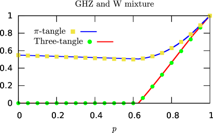
Figure 1: Three-tangle and $\pi$-tangle calculated for states $\rho_{p}$. Symbols (boxes and circles) and continuous lines represent numerical and analytical values, respectively.

Figure 2: Three-tangle and $\pi$-tangle calculated for states $\rho^{\prime}_{p}$. Symbols (boxes and circles) and the continuous line represent numerical and analytical values, respectively.

The three-tangle and $\pi$-tangle measures can be used to discriminate among the classes $B$, $W\backslash B$ and $GHZ\backslash W$ Ou and Fan (2007). For the family of states $2\rho_{p}$, the analytical results in Lohmayer et al. (2006); Eltschka et al. (2008), and described in Appendix A, show that $\rho_{p}$ belongs to the $W\backslash B$ class for $p\lesssim 0.62685$ and to the $GHZ\backslash W$ class for higher values of $p$. As show by Fig. 1, the positive values of the three-tangle indicate the $GHZ\backslash W$ class, whereas the positive values of the $\pi$-tangle in the region where the three-tangle is zero show that the state belongs to the $W\backslash B$ class. The graph around the class transition point, calculated with a tolerance $\epsilon=10^{-5}$ and depicted in Fig. 3, shows that the numerical result is in a good agreement with the analytical one. In the case of the family $\rho^{\prime}_{p}$, it belongs to the $B$ class for $p\leq p_{B}\equiv 3/7\approx 0.42857$, to the $W\backslash B$ class for $3/7<p\leq p_{W}\approx 0.69554$ and to the $GHZ\backslash W$ class for $p>p_{W}$ Gühne and Seevinck (2010); Eltschka and Siewert (2012). The plot in Fig. 4 shows that the class transition in $p_{B}$ occurs between $p=0.43$ and $p=0.44$, which is only slightly higher than $p_{B}$, which is expected since the algorithm gives a close lower bound to the optimal value. In addition, the numerical values in the graph show the transition between classes $W\backslash B$ and $GHZ\backslash W$.

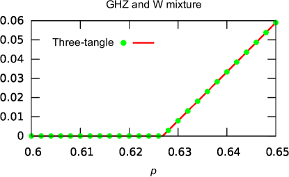
Figure 3: Three-tangle calculated for states $\rho_{p}$. Symbols (circles) and the continuous line represent numerical and analytical values, respectively.

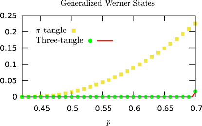
Figure 4: Three-tangle and $\pi$-tangle calculated for states $\rho^{\prime}_{p}$. Symbols (boxes and circles) and the continuous line represent numerical and analytical values, respectively.

V Conclusion

We explored the theory of LSIP to derive properties of the dual problem of the convex roof procedure that gives entanglement monotones for mixed states from pure state measures. We showed that the absence of the duality gap between primal and dual problems occurs in very general conditions. In addition, we proved that the set of optimal points is non-empty and bounded and we derived bounds on the coefficients of optimal solutions. For numerical calculations, we wrote the dual problem in a suitable LSIP form and described the pseudocode of an CCPA designed for this type of optimization. To check the performance of the algorithm, we calculated two measures of genuine three-qubit entanglement, three-tangle and $\pi$-tangle, for the mixture of GHZ and W states and for the generalized Werner states, a full rank family of states. We compared the numerical results with the available analytical values and verified that the CCPA results are very close the exact ones for the lower rank family of states, while providing lower bounds for the high rank ones. As the algorithm gives lower bounds on the amount of entanglement for suboptimal feasible points and global convergence, the results are in agreement with the expected behavior. Furthermore, we used the difference between the two measures to distinguish $GHZ\backslash W$ and $W$ classes, in agreement with the entanglement classification of these states in the literature.

We believe that our work gives a good alternative to the convex roof calculation of mixed states entanglement, especially when close lower bounds are required. The CCPA has very general applicability, working with discontinuous measures and multipartite states with any finite rank. For future works, we expect to apply other LSIP algorithms to the convex roof problem, with the necessary modifications and improvements.

Appendix A Thee-tangle and $\pi$-tangle for families of states

Here, we show the analytical expressions for the three-tangle and $\pi$-tangle for the families of states $\rho_{p}$ and $\rho^{\prime}_{p}$ available in the literature. First, we show the formulas for the three-tangle quantifier applied to the mixture of GHZ and W states: $\rho_{p}$. Set $s\equiv 8\sqrt{6}/9$, $p_{0}\equiv s^{2/3}/(1+s^{2/3})$, $p_{1}\equiv 1/2+1/\big{(}2\sqrt{1+s^{2}}\big{)}$. The three-tangle of $\rho_{p}$ is given by Lohmayer et al. (2006); Eltschka et al. (2008)

$$\tau(\rho_{p})=\Bigg{\{}\begin{matrix}0&\text{for $p\leq p_{0}$,}\\ \tau_{3}(p,0)&\hskip 14.22636pt\text{for $p_{0}<p\leq p_{1}$,}\\ \hskip 2.84544pt\tau_{3}^{\text{conv}}(p,p_{1})&\text{for $p>p_{1}$,}\end{matrix}$$ (7)

where $\tau_{3}(p,0)\equiv\big{\arrowvert}p^{2}-16\sqrt{p(1-p)^{3}}/3\sqrt{6}\big{\arrowvert}$ and $\tau_{3}^{\text{conv}}(p,p_{1})\equiv\big{[}p-p_{1}+(1-p)\big{(}p_{1}^{2}-s\sqrt{p_{1}(1-p_{1})^{3}}\big{)}\big{]}/(1-p_{1})$.

The family of states $\rho^{\prime}_{p}$, as the parameter $p$ ranges from 0 to 1, goes through all three-qubit entanglement classes: $S,B\backslash S,W\backslash B$ and $GHZ\backslash W$ Eltschka and Siewert (2012), where $S$ is the class of separable states. The value $p_{W}$ of $p$ that separates the classes $W$ and $GHZ\backslash W$ is $p_{W}\approx 0.6955427$. The three-tangle of $\rho^{\prime}_{p}$ is then given by Siewert and Eltschka (2012)

$$\tau(\rho^{\prime}_{p})=\bigg{\{}\begin{matrix}0&\text{for $p\leq p_{W}$,}\\ \hskip 2.84544pt\frac{p-p_{W}}{1-p_{W}}&\hskip 18.49411pt\text{for $p_{W}<p\leq 1$.}\end{matrix}$$ (8)

The last available analytical result is the $\pi$-tangle of the states $\rho_{p}$, which is given by MA and FEI (2013):

$$\pi(\rho_{p})=\Bigg{\{}\begin{matrix}\pi^{(1)}(\rho_{p})&\text{for $0\leq p\leq p_{0}$,}\\ \pi^{(2)}(\rho_{p})&\text{for $p_{0}<p\leq p_{1}$,}\\ \pi^{(3)}(\rho_{p})&\text{for $p_{1}<p\leq 1$,}\end{matrix}$$ (9)

where $\pi^{(1)}(\rho_{p})\equiv\big{\{}4(\sqrt{5}-1)(p_{0}-p)+p\big{[}5p_{0}^{2}-4p_{0}+8-18\big{(}\sum_{i=1}^{4}|\lambda_{i}(p_{0})|-1\big{)}^{2}\big{]}\big{\}}/9p_{0}$, $\pi^{(2)}(\rho_{p})\equiv\big{[}5p^{2}-4p+8-18\big{(}\sum_{i=1}^{4}|\lambda_{i}(p)|-1\big{)}^{2}\big{]}/9$ and $\pi^{(3)}(\rho_{p})\equiv\big{\{}p-p_{1}+(1-p)\big{[}5p_{1}^{2}-4p_{1}+8-18\big{(}\sum_{i=1}^{4}|\lambda_{i}(p_{1})|-1\big{)}^{2}\big{]}/9\big{\}}/(1-p_{1})$. For a fixed value of $p$, each $\lambda_{i}(p)$, for $i\in\{1,\ldots,4\}$, is a solution of the following equation:

$$\lambda^{4}-\lambda^{3}+\left(\frac{5}{36}p^{2}-\frac{p}{9}+\frac{2}{9}\right)\lambda^{2}+\bigg{[}\frac{(p(1-p))^{3/2}}{3\sqrt{6}}$$

$$-\frac{7}{27}p^{3}+\frac{7}{18}p^{2}-\frac{p}{6}+\frac{1}{27}\bigg{]}\lambda+\bigg{[}-\frac{p(p(1-p))^{3/2}}{6\sqrt{6}}$$

$$-\frac{41}{648}p^{4}+\frac{149}{648}p^{3}-\frac{13}{54}p^{2}+\frac{7}{81}p-\frac{1}{81}\bigg{]}=0.$$

Appendix B Bounding the feasible set

Lemma 1.

If $0\leq E([\psi])\leq 1,\forall[\psi]\in\mathcal{E}_{\rho},$ and $\delta\equiv(r-1)\lambda_{r}/\lambda_{1}$, where $r=\operatorname{rank}(\rho)$, $\lambda_{1}$ and $\lambda_{r}$ are the lowest and highest eigenvalues of $\rho$, respectively, then $F_{\rho}^{\ast}\subseteq B_{\delta}$.

Proof.

Let $x_{1}\leq\ldots\leq x_{r}$ be the eigenvalues of $X\in H_{\rho}$. By the constraint $E([\psi])+\operatorname{Tr}([\psi]X)\geq 0,\forall[\psi]\in\mathcal{E}_{\rho}$, of the problem $D_{\rho}$ and the min-max theorem, we have that $x_{1}\geq-1$ is a necessary condition for the feasibility of $X$. Let $\{|x_{1}\rangle,\ldots|x_{r}\rangle\}$ be an orthonormal basis with eigenvectors of $X$ and $\rho=\sum_{k,l}\lambda_{k,l}^{\prime}|x_{k}\rangle\langle x_{l}|$. As $x_{1}\geq-1$, $0\leq E^{\cup}(\rho)\leq 1$ and by the fact that there is no duality gap between $D_{\rho}$ and $P$, if $X\in F_{\rho}^{\ast}$ then

$$\operatorname{Tr}(\rho X)=\sum_{k}\lambda_{k,k}^{\prime}x_{k}\leq 0\Rightarrow x_{r}\leq(r-1)\frac{\lambda_{r}}{\lambda_{1}}.$$ (10)

Equation 10 implies that $\|X\|=\sup\{\|X|\psi\rangle\|_{2}:\||\psi\rangle\|_{2}=1\}=\max\{|x_{1}|,|x_{r}|\}\leq(r-1)\lambda_{r}/\lambda_{1}$. Thus, we conclude that $F_{\rho}^{\ast}\subseteq B_{\delta}$ for $\delta\equiv(r-1)\lambda_{r}/\lambda_{1}$. ∎

Corollary 1.

Let $\{Z_{1},\ldots,Z_{r^{2}}\}$ be an orthonormal basis of $H_{\rho}$, $r=\operatorname{rank}(\rho)$ and $\lambda_{1}\leq\ldots\leq\lambda_{r}$ the eigenvalues of $\rho$. If $X\in F_{\rho}^{\ast}$ then $x_{m}^{\prime}\equiv|\operatorname{Tr}(A_{m}X)|\leq r(r-1)\lambda_{r}/\lambda_{1}$.

Proof.

Let $\{|x_{1}\rangle,\ldots|x_{r}\rangle\}$ be an orthonormal basis with eigenvectors of $X$ and $X=\sum_{k}x_{k}[x_{k}]$. By Lemma 1, $|\operatorname{Tr}(Z_{m}X)|\leq\sum_{k}|x_{k}||\operatorname{Tr}(Z_{m}[x_{k}])|\leq\sum_{k}|x_{k}|\leq r(r-1)\lambda_{r}/\lambda_{1}$. ∎

References

- Horodecki et al. (2009) R. Horodecki, P. Horodecki, M. Horodecki, and K. Horodecki, Rev. Mod. Phys. 81, 865 (2009).
- Vidal (2000) G. Vidal, J. Mod. Opt. 47, 355 (2000), arXiv:9807077v2 [arXiv:quant-ph] .
- Życzkowski (1999) K. Życzkowski, Phys. Rev. A 60, 3496 (1999).
- Audenaert et al. (2001) K. Audenaert, F. Verstraete, and B. De Moor, Phys. Rev. A 64, 052304 (2001).
- Röthlisberger et al. (2009) B. Röthlisberger, J. Lehmann, and D. Loss, Phys. Rev. A 80, 042301 (2009).
- Cao et al. (2010) K. Cao, Z.-W. Zhou, G.-C. Guo, and L. He, Phys. Rev. A 81, 034302 (2010).
- Röthlisberger et al. (2012) B. Röthlisberger, J. Lehmann, and D. Loss, Comput. Phys. Commun. 183, 155 (2012).
- Ryu et al. (2012) S. Ryu, S.-S. B. Lee, and H.-S. Sim, Phys. Rev. A 86, 042324 (2012).
- Tóth et al. (2015) G. Tóth, T. Moroder, and O. Gühne, Phys. Rev. Lett. 114, 160501 (2015).
- Brandão (2005) F. G. S. L. Brandão, Phys. Rev. A 72, 022310 (2005).
- Bengtsson and Zyczkowski (2006) I. Bengtsson and K. Zyczkowski, “Geometry of Quantum States,” (Cambridge University Press, Cambridge, 2006) Chap. 17, pp. 493–543, 2nd ed.
- Bruß and Macchiavello (2011) D. Bruß and C. Macchiavello, Phys. Rev. A 83, 052313 (2011).
- Pan et al. (2017) M. Pan, D. Qiu, and S. Zheng, Quantum Inf. Process. 16, 211 (2017).
- Cabello (2000) A. Cabello, (2000), arXiv:0009025 [quant-ph] .
- Epping et al. (2017) M. Epping, H. Kampermann, C. Macchiavello, and D. Bruß, New J. Phys. 19, 093012 (2017).
- Murta et al. (2020) G. Murta, F. Grasselli, H. Kampermann, and D. Bruß, (2020), arXiv:2003.10186 .
- Greenberger et al. (1990) D. M. Greenberger, M. A. Horne, A. Shimony, and A. Zeilinger, Am. J. Phys. 58, 1131 (1990).
- Hauke et al. (2016) P. Hauke, M. Heyl, L. Tagliacozzo, and P. Zoller, Nat. Phys. 12, 778 (2016).
- Smith et al. (2016) J. Smith, A. Lee, P. Richerme, B. Neyenhuis, P. W. Hess, P. Hauke, M. Heyl, D. A. Huse, and C. Monroe, Nat. Phys. 12, 907 (2016).
- Coffman et al. (2000) V. Coffman, J. Kundu, and W. K. Wootters, Phys. Rev. A 61, 052306 (2000).
- MIYAKE (2004) A. MIYAKE, Int. J. Quantum Inf. 02, 65 (2004).
- Ou and Fan (2007) Y.-C. Ou and H. Fan, Phys. Rev. A 75, 062308 (2007).
- Guo and Zhang (2020) Y. Guo and L. Zhang, Phys. Rev. A 101, 032301 (2020).
- Hill and Wootters (1997) S. Hill and W. K. Wootters, Phys. Rev. Lett. 78, 5022 (1997).
- Lohmayer et al. (2006) R. Lohmayer, A. Osterloh, J. Siewert, and A. Uhlmann, Phys. Rev. Lett. 97, 260502 (2006).
- Eltschka et al. (2008) C. Eltschka, A. Osterloh, J. Siewert, and A. Uhlmann, New J. Phys. 10, 043014 (2008).
- Siewert and Eltschka (2012) J. Siewert and C. Eltschka, Phys. Rev. Lett. 108, 230502 (2012).
- Vidal and Werner (2002) G. Vidal and R. F. Werner, Phys. Rev. A 65, 032314 (2002).
- Vedral et al. (1997) V. Vedral, M. B. Plenio, M. A. Rippin, and P. L. Knight, Phys. Rev. Lett. 78, 2275 (1997).
- Eisert et al. (2007) J. Eisert, F. G. S. L. Brandão, and K. M. R. Audenaert, New J. Phys. 9, 46 (2007).
- Reemtsen and Rückmann (1998) R. Reemtsen and J.-J. Rückmann, eds., Semi-Infinite Programming, 1st ed., Nonconvex Optimization and Its Applications, Vol. 25 (Springer US, Boston, MA, 1998).
- Goberna and López (1998) M. A. Goberna and M. A. López, Linear Semi-Infinite Optimization, edited by B. Brosowski and G. F. Roach (John Wiley & Sons, 1998).
- Terhal and Horodecki (2000) B. M. Terhal and P. Horodecki, Phys. Rev. A 61, 040301 (2000).
- Lee and Sim (2012) S.-S. B. Lee and H.-S. Sim, Phys. Rev. A 85, 022325 (2012).
- Horodecki et al. (2001) M. Horodecki, P. Horodecki, and R. Horodecki, Phys. Lett. A 283, 1 (2001).
- Terhal (2002) B. M. Terhal, Theor. Comput. Sci. 287, 313 (2002).
- Goberna and López (2017) M. A. Goberna and M. A. López, 4OR 15, 221 (2017).
- Gribik (1979) P. R. Gribik, in Semi-Infinite Program., edited by R. Hettich (Springer-Verlag, Berlin/Heidelberg, 1979) pp. 66–82.
- Betrò (2004) B. Betrò, Math. Program. 101, 479 (2004).
- MA and FEI (2013) T. MA and S.-M. FEI, in Quantum Bio-Informatics V - Proc. Quantum Bio-Informatics 2011, Vol. 30, edited by L. Accardi, W. Freudenberg, and M. Ohya (World Scientific Publishing Co. Pte. Ltd., 2013) pp. 425–434.
- Gühne and Seevinck (2010) O. Gühne and M. Seevinck, New J. Phys. 12, 053002 (2010).
- Eltschka and Siewert (2012) C. Eltschka and J. Siewert, Phys. Rev. Lett. 108, 020502 (2012).