Saliency Prediction with External Knowledge

Abstract

The last decades have seen great progress in saliency prediction, with the success of deep neural networks that are able to encode high-level semantics. Yet, while humans have the innate capability in leveraging their knowledge to decide where to look (e.g. people pay more attention to familiar faces such as celebrities), saliency prediction models have only been trained with large eye-tracking datasets. This work proposes to bridge this gap by explicitly incorporating external knowledge for saliency models as humans do. We develop networks that learn to highlight regions by incorporating prior knowledge of semantic relationships, be it general or domain-specific, depending on the task of interest. At the core of the method is a new Graph Semantic Saliency Network (GraSSNet) that constructs a graph that encodes semantic relationships learned from external knowledge. A Spatial Graph Attention Network is then developed to update saliency features based on the learned graph. Experiments show that the proposed model learns to predict saliency from the external knowledge and outperforms the state-of-the-art on four saliency benchmarks.

1 Introduction

Visual attention is the ability to select the most relevant part of the visual input. It helps humans to rapidly process the overwhelming amount of visual information acquired from the environments. Saliency prediction is a computational task that models the visual attention driven by the visual input [20], which has wide applicability in different domains, such as image quality assessment [55], robot navigation [8] and video surveillance [37], and screening neurological disorders [24, 48, 49].

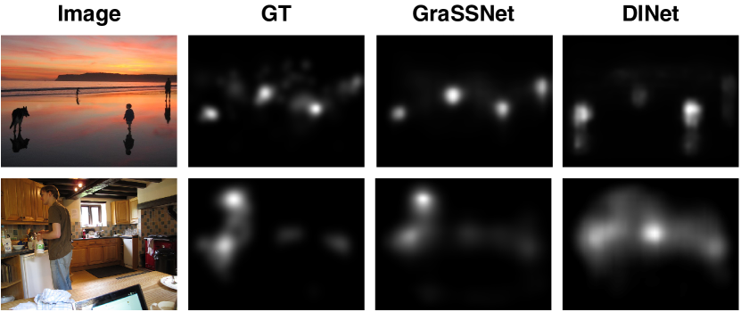
Figure 1: Examples of how semantic proximity affects saliency maps. External semantic relationships are effective in deciding the relative saliency of objects

Where humans look is involuntarily influenced by their prior knowledge. Such knowledge can be general commonsense knowledge or specific ones that require prior experience or training [9, 19, 33]. It is commonly noticed that salient objects tend to influence the saliency of similar objects. For example, as illustrated in Fig. 1, when multiple people and objects exist, their saliency values relevant to the closeness of their relationships. When one of them is salient, their related objects also tend to be salient.

Differently, despite the success of deep neural networks for saliency prediction [4, 18, 31], they rely on training data and learn ‘knowledge’ only in a data-driven and implicit manner. With the advancement of DNNs and the collection of more data, these networks learn better semantics that encode objects and maybe high-level context or relationship; it is, however, unclear to what degree what knowledge can be learned, and it heavily depends on the data quantity and content. Therefore, we in this work propose to leverage ground truth knowledge from external sources. Such knowledge could well complement the features learned from the neural networks to more intelligently decide where to look. Note that attention data are not trivial to scale [39], which makes this work more useful in practice, e.g. domain-specific knowledge could be directly used to guide saliency prediction in a clinical application without big attention ground truth.

To demonstrate the overarching goal, we use two external knowledge sources (MSCOCO image captioning [35] and WordNet [38]) that describe semantic relationships between objects. Semantic relationship is important to saliency prediction as objects are correlated and together they also reflect context; it is also one of the most well-structured and documented sources of external knowledge. We introduce this knowledge into a computational saliency model by designing a Graph Semantic Saliency Network (GraSSNet), which explicitly analyzes the semantic relationships of objects in a scene and uses such knowledge for saliency prediction. In particular, we propose a Semantic Proximity Network (SPN) that computes the semantic proximity of detected region proposals in semantic spaces of interest. While external knowledge is explicitly used to supervise the learning of the network, the relationships to be distilled is dependent on the input image by setting the distillation loss as a part of the objective. We further propose a Spatial Graph Attention Network (sGAT) to propagate the semantic features of region proposals based on their semantic proximity with maintained latent spatial structures, where the updated features will be used together with the multi-scale spatial feature maps to compute saliency maps.

In sum, we propose to explicitly leverage external knowledge for saliency prediction, as a complementary source of information to neural network based models. Extensive experiments on four datasets with comparisons with six models and analyses demonstrate the advantage of incorporating the knowledge. The main technical contributions are summarized as follows:

• We propose a new graph-based saliency prediction model by leveraging object-level semantics and their relationships.

• We propose a novel Semantic Proximity Network to explicitly distill semantic proximity from multiple external knowledge bases for saliency prediction.

• We propose Spatial Graph Attention Network to dynamically propagate semantic features across objects for the prediction of the saliency across multiple objects.

2 Related Works

In this section, we first review state-of-the-art visual saliency models. Next, we briefly introduce how external knowledge is utilized in other high-level computer vision tasks (e.g. relationship detection) and how we adapt it to predict saliency. Lastly, we review and compare graph convolution methods with ours.

2.1 Deep Saliency Prediction Models

The recent success of deep learning models has brought considerable improvements in saliency prediction tasks. One of the first work is Ensemble of Deep Networks (eDN) [47], which combines multiple features from a few convolution layers. Later DeepGaze I [32] leverages a deeper structure for better feature extraction. After that, many models [21, 29, 30] follow the framework that consists of a deep model and fully convolutional networks (FCN) to leverage the powerful capabilities in contextual feature extraction. These models are often pre-trained on large datasets (e.g. SALICON [23]) and then fine-tuned on small-scale fixation datasets. However, with the increasing model depth, many downsampling operations are performed, contributing to a lower spatial resolution and limited performance [36]. A recent state-of-the-art model named Dilated Inception Networks (DINet) [52] leverages dilated convolutions to tackle the issue. Another major strength of the deep model is its capabilities of high-level feature extraction. Many deep neural network based method [4, 18, 23, 31] have boosted saliency prediction performance by implicitly encoding semantics with different approaches (e.g. subnets in different scales [18], inception blocks [44], etc.).

However, none of the previous methods explored the saliency patterns among different objects in a scene. Our model differentiates itself from existing methods by leveraging the relationships of various semantics for saliency prediction, using a Semantic Proximity Network and a Spatial Graph Attention Network.

2.2 External Knowledge Distillation

External knowledge has gained great interest in natural language processing [3, 17] and computer vision [1, 11, 34]. As the information extracted from training sets are always insufficient to fully recover the real knowledge domain, previous works explicitly incorporate external knowledge to compensate it. Generally, there are two commonly used frameworks for knowledge distillation.

One framework is teacher-student distillation. For example, Yu et al. [53] leverages this structure to absorb linguistic knowledge in visual relationship detection tasks. Apart from the teacher-student structure, more existing works in object/relationship detection and scene graph generation adopt the graph framework. For instance, KG-GAN [13] improves the performance of scene graph generation by effectively propagating contextual information across the external knowledge graph. Similarly,  [22] adopts external knowledge graphs to solve the long-tail problems in object detection tasks.

Our model also employs a graph framework to distill external knowledge. However, unlike object/relationship detection tasks, where semantics are explicitly defined and structured (e.g. objects, relationships), semantics in saliency feature maps are always entangled, making them non-trivial to connect with external knowledge. To tackle this problem, we not only segment semantics by extracting region proposals, but also convert the external knowledge to image specific region-to-region semantic proximity graphs.

2.3 Graph Convolution Networks

Leveraging graphs in saliency prediction has been explored at the pixel level. GBVS [15] treats every pixel as node and diffuses its saliency information along the edges by Markov chains. Recently, graph convolution networks have been applied in various tasks that require information propagation. These methods can largely be categorized into spectral [5, 16, 27] and non-spectral [2, 12, 14] approaches. One recent approach named Graph Attention Network (GAT)[46] achieves state-of-the-art by leveraging self-attention mechanism.

Inspired by the GAT, we develop a Spatial Graph Attention Network (sGAT) to process spatial feature maps as node attributes. While SGAT assumes no spatial structure within node attributes, our proposed sGAT encodes spatial characteristics during feature propagation, because of their importance in predicting the spatial distribution of attention.

3 Method

This section presents the Graph Semantic Saliency Network (GraSSNet), as shown in Fig. 2. The task is formulated as follows: given a 2D image $I$ as the input, it aims to construct a semantic proximity graph and use it to predict a saliency map as a 2D probability distribution of eye fixations. We will first describe our model architecture, followed by the details of the two novel components: Semantic Proximity Network (SPN) and Spatial Graph Attention Network (sGAT). Finally, we present the objective function to optimize our model.

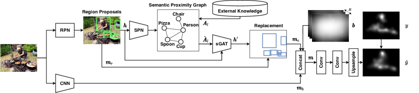
Figure 2: Architecture of the proposed graph semantic saliency network. The architecture mainly consists of a Region Proposal Network (RPN), a Semantic Proximity Network (SPN), a Spatial Graph Attention Network (sGAT), and a baseline saliency network. The concatenated features from external knowledge (top), baseline saliency network (bottom) and prior maps (optional) are fed into several convolutional and upsampling layers to compute saliency maps

3.1 Model Architecture

Object Feature Retrieval. Our method is based on detected region proposals. As shown in Fig. 2, the model uses a pre-trained Faster R-CNN [42] to detect all objects from the input image $I$, generating a set of bounding boxes $B=\{b_{1},\cdots,b_{p}\}$ where $p$ denotes the total number of detected instances. Their corresponding regional features ${\boldsymbol{h}}=\{h_{1},h_{2},\cdots,h_{p}\}$, $h_{i}\in\mathbb{R}^{d_{1}\times d_{2}\times d_{3}}$ are extracted from the outputs of the ROI pooling layer, where $d_{1}$, $d_{2}$ and $d_{3}$ denote the dimensions of features.

Semantic Proximity Graph Construction. To incorporate external knowledge from multiple sources, we process these regional features with a set of $N$ Semantic Proximity Networks (SPNs) that predict the semantic proximity graphs under the supervision from $N$ different external knowledge sources. This design makes it flexible to extend the model with additional knowledge bases. Given regional features ${\boldsymbol{h}}$, a semantic proximity graph is computed as

$$\hat{{\boldsymbol{A}}}_{l}=f_{\text{SPN}}^{l}({\boldsymbol{h}}),$$ (1)

where $f_{\text{SPN}}^{l}$ denotes the SPN supervised by an external knowledge graph ${\boldsymbol{A}}_{l}$ where $l=1,\cdots,N$.

Semantic Proximity Knowledge Distillation. Upon obtaining $N$ predicted graphs $\hat{{\boldsymbol{A}}}=\{\hat{{\boldsymbol{A}}}_{1},\hat{{\boldsymbol{A}}}_{1},\cdots,\hat{{\boldsymbol{A}}}_{N}\}$, the regional features are processed with $N$ different Graph Attention Networks (sGATs), sharing the saliency features to their immediate neighbors in the corresponding semantic proximity graphs to generate updated regional features ${\boldsymbol{h}}^{\prime}_{l}=\{h^{\prime}_{l1},h^{\prime}_{l2},\cdots,h^{\prime}_{lp}\}$:

$${\boldsymbol{h}}^{\prime}_{l}=f_{\text{sGAT}}^{\hat{{\boldsymbol{A}}_{l}}}({\boldsymbol{h}}).$$ (2)

By supervising the SPNs with different externally built ground-truth proximity graphs, diverse proximity knowledge can be learned from external knowledge, so that features can be propagated along the predicted graphs.

We concatenate all the updated regional features $\{{\boldsymbol{h}}^{\prime}_{l}\},\,l\in[1,2,\cdots,N]$ and use a convolution layer to compute the final updated features ${\boldsymbol{h}}^{\prime}$, which are projected back to replace the raw map features ${\boldsymbol{m}}_{r}$ in the detected bounding boxes. Features in overlapping regions are merged with the max operation.

Prior Maps Generation. As fixations tend to be biased towards the center of the image [45], we model this center bias ${\boldsymbol{b}}$ and combine it into the saliency map. Specifically, our model learns a total of $R$ Gaussian prior maps from the data to model the center bias, whose means ($\mu_{x},\mu_{y}$) and variances ($\sigma_{x}^{2},\sigma_{y}^{2}$) are learned as follows:

$$f_{\text{gau}}(x,y)=\frac{1}{2\pi\sigma_{x}\sigma_{y}}\exp(-(\frac{(x-\mu_{x})^{2}}{2\sigma_{x}^{2}}+\frac{(y-\mu_{y})^{2}}{2\sigma_{y}^{2}})).$$ (3)

Saliency Map Generation. Consequently, the saliency maps are constructed by concatenating spatial feature map ${\boldsymbol{m}}_{e}$, baseline feature map ${\boldsymbol{m}}_{b}$ and prior maps ${\boldsymbol{b}}$:

$$\hat{y}=f_{\text{end}}({\boldsymbol{m}}_{e}\mathbin{\|}{\boldsymbol{m}}_{b}\mathbin{\|}{\boldsymbol{b}}),$$ (4)

where $\mathbin{\|}$ denotes the concatenation operations and $f_{\text{end}}$ represents two convolution layers and one bilinear upsampling layer.

In the rest of this section, we describe two key components of the architecture.

3.2 Semantic Proximity Network

A key component of our model is the explicit modeling of semantic proximity, with the supervision from external knowledge. As shown in Fig. 3, the computation of an external proximity graph consists of two steps. First, we propose a Semantic Proximity Network (SPN) that predicts the semantic proximity graph based on the input features. Each node in the semantic proximity graph represents a detected object, and the edges indicate their pairwise semantic proximity. Next, we build an external knowledge graph from semantic databases (e.g. MSCOCO captions, WordNet), which models the semantic proximity between different object categories. While the external knowledge graph is used as the explicit supervision of the SPN, the distillation is not forced. Instead, with the distillation loss as a part of the model objective, the model can learn various semantic relationships, and how to incorporate such information is dependent on the input image. To include richer semantic proximity information, multiple knowledge graphs can be incorporated with different SPNs.

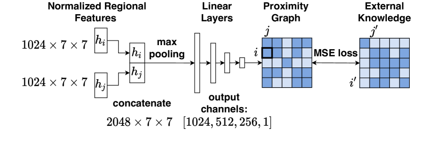
Figure 3: Learning of the Semantic Proximity Network. Region-to-region semantic proximity values are predicted by feeding concatenated regional features to a four-layer MLP. The weights of SPN are trained under the supervision of external object relationship knowledge with a MSE loss

We define the $l$-th semantic proximity graph as a $p\times p$ adjacency matrix ${\boldsymbol{\hat{A}_{l}}}$, and $\hat{e}_{ij}$ represents the learned edge connectivity between region $i$ and region $j$, where $p$ is the number of regions. The SPN aims to predict the edge connectivity between every two regions. Specifically, as shown in Fig. 3, the edge $\hat{e}_{ij}$ of specific graph’s adjacency matrix ${\boldsymbol{\hat{A}}}_{l}$ can be computed with a Multi-Layer Perceptron (MLP):

$$\hat{e}_{ij}=\text{MLP}_{{\boldsymbol{\hat{A}}}_{l}}(h_{i}\mathbin{\|}h_{j}),$$ (5)

where $\mathbin{\|}$ represents the concatenation operation. If $\hat{e}_{ij}$ is greater than a threshold $\theta_{l}$, an edge is formed between region $i$ and region $j$.

To supervise the learning of each SPN, we construct external knowledge graphs of semantic proximity. The proximity information can be obtained from multiple sources. Details about building external knowledge graphs will be discussed in Implementation Details (Section 4.3).

3.3 Spatial Graph Attention Network

We propose a Spatial Graph Attention Network (sGAT) to use the distilled external knowledge (i.e., semantic proximity graph) for saliency prediction. The sGAT is composed of multiple graph convolutional layers. The inputs to the sGAT are the regional features ${\boldsymbol{h}}=\{h_{1},h_{2},\cdots,h_{p}\}$, while its output is a group of updated regional features ${\boldsymbol{h}}_{l}^{\prime}=\{h^{\prime}_{l1},h^{\prime}_{l2},\cdots,h^{\prime}_{lp}\}$, $h^{\prime}_{li}\in\mathbb{R}^{d_{1}\times d_{2}\times d_{3}}$. The sGAT computes attention coefficients $c_{ij}$, where $i,j$ are the indices of the regions.

To predict saliency, it is important to preserve the spatial characteristics of the region proposals. Therefore, different from the standard GAT method, in this work $c_{ij}$ is computed as

$$c_{ij}=f_{\text{att}}({\boldsymbol{W}}\circ h_{i},{\boldsymbol{W}}\circ h_{j}),$$ (6)

where ${\boldsymbol{W}}$ are learnable weights of a spatial filter, $\circ$ denotes the convolution operation, and $f_{\text{att}}$ represents an attention block following GAT [46]. The sGAT computes the coefficients of the region $i$’s immediate neighbors (include $i$) in the predicted semantic proximity graph. With a softmax normalization on $c_{ij}$, we obtain attention values $\{\alpha_{ij}\}$, indicating region $j$’s importance towards region $i$.

Finally, we obtain an updated node features $h^{\prime}_{li}$ by linearly combining convoluted features from node $i$’s neighboring nodes with attention values as weights. We adopted a multi-head strategy to stabilize the learning process:

$$h^{\prime}_{li}=\mathbin{\|}_{k=1}^{K}\sigma(\sum_{j\in N_{i}}\alpha_{ij}{\boldsymbol{W}}\circ h_{j}),$$ (7)

where $\mathbin{\|}$ represents concatenation and $K=8$ is the number of attention heads.

3.4 Objective

In this work, we aim to jointly optimize the saliency prediction and the prediction of semantic proximity graph. Therefore, our model is optimized with two objective functions: the saliency prediction loss and the semantic proximity loss.

For the saliency prediction, our model is trained with a linear combination of $L_{1}$ loss following [52]) and two of the most recommended saliency evaluation metrics [7] CC and NSS. They complement each other and together ensure the model’s overall performance:

$$L_{\text{sal}}=L_{1}(\hat{y},y)-\beta L_{CC}(\hat{y},y)-\gamma L_{NSS}(\hat{y},y),$$ (8)

where $\hat{y}$ denotes the output saliency map and the ground truth is denoted as $y$.

To supervise the predicted semantic proximity graph $\hat{{\boldsymbol{A}}}_{l}$, we need to leverage instance labels in the training phase. Assume we are going to predict the connectivity between region $i$ and region $j$, we can find their corresponding class $i^{\prime}$ and $j^{\prime}$ based on the positions. Next, we retrieve the corresponding ground truth edge connectivity $e_{i^{\prime}j^{\prime}}$ from ${\boldsymbol{A}}_{l}$. Note that $\hat{{\boldsymbol{A}}}_{l}$ is in $m\times m$, while ${\boldsymbol{A}}_{l}$ is in $p\times p$, where $m$ is the number of proposed regions and $p$ is the number of classes from external knowledge. We generate multiple proximity graphs with different semantics with the mean squared error (MSE) loss:

$$L_{\text{prox}}=\sum_{0<=i<j<p}(\hat{e}_{ij}-e_{i^{\prime}j^{\prime}})^{2}.$$ (9)

The final loss is the linear combination between saliency prediction loss and semantic proximity loss:

$$L=L_{\text{sal}}+\lambda L_{\text{prox}}.$$ (10)

4 Experiments

This section reports extensive comparative experiments and analyses. We first introduce the datasets, evaluation metrics, and implementation details. Next, we quantitatively compare our proposed method to the state-of-the-art saliency prediction methods. Finally, we conduct ablation studies to examine the effect of each proposed component, and present qualitative results.

4.1 Saliency Datasets

We evaluate our models on four public saliency datasets: SALICON [23] is the largest available dataset for saliency prediction. It contains 10,000 training images, 5,000 validation images and 5,000 testing images, all selected from the MSCOCO dataset [35]. It provides ground-truth fixation maps by simulating eye-tracking with mouse movements. MIT1003 [25] includes 1,003 natural indoor and outdoor scenes, with 779 landscape and 228 portrait images. The eye fixations are collected from 15 observers aged between 18 to 35. CAT2000 [6] contains 4,000 images from 20 different categories, which are collected from a total of 120 observers. The dataset is divided into two sets, with 2,000 images in the training set and the rest in the test set. OSIE [51] consists of 700 indoor and outdoor scenes from Flickr and Google, with fixations collected from 15 observers between 18 to 30. The dataset has a total of 5,551 segmented objects with fine contours.

4.2 Evaluation Metrics

Metrics to evaluate saliency prediction performance can be classified into two categories: distribution-based metrics and location-based metrics [7, 43].

We evaluate saliency models with three location-based metrics. One of the most universally accepted location-based metrics is the Area Under the ROC curve (AUC) [25], which treats each pixel at the saliency map as a classification task. To take into account the center bias in eye fixations, we also use the shuffled AUC (sAUC) [54] that draws negative samples from fixations in other images. Another widely used metric is Normalized Scanpath Saliency (NSS) [41], which is computed as the average normalized saliency at fixated locations.

We also use three distribution-based metrics for model evaluation. One is the Linear Correlation Coefficient (CC) [7]. The CC metric is computed by dividing the covariance between predicted and ground-truth saliency map with ground truth. Besides, the similarity metric (SIM) [7] is also adopted to measure the similarity between two distributions. We also computed Kullback-Leibler divergence (KL) [7] that measures the difference between two distributions from the perspective of information theory.

Table 1: Evaluation results of the the compared models. RED and BLUE indicate the best performance and the second best. The proposed model is compared with six state-of-the-art models on SALICON, MIT1003, CAT2000 and OSIE datasets under six evaluation metrics. Respectively, GraSSNet+CB and GraSSNet denote the model with and without prior map generation as center bias

	SALICON							MIT1003
Methods	CC	AUC	NSS	sAUC	KL	SIM		CC	AUC	NSS	sAUC	KL	SIM
GraSSNet+CB	0.866	0.892	3.292	0.784	0.604	0.812		0.775	0.910	2.921	0.629	0.574	0.595
GraSSNet	0.867	0.888	3.261	0.786	0.598	0.805		0.772	0.909	2.897	0.641	0.633	0.577
DINet [52]	0.860	0.884	3.249	0.782	0.613	0.804		0.764	0.907	2.851	0.635	0.690	0.561
SAM-Res [10]	0.842	0.883	3.204	0.779	0.607	0.791		0.768	0.913	2.893	0.617	0.684	0.543
SAM-VGG [10]	0.825	0.881	3.143	0.774	0.610	0.793		0.757	0.910	2.852	0.613	0.676	0.568
DSCLRCN [36]	0.831	0.884	3.157	0.776	0.637	0.731		0.749	0.882	2.817	0.621	0.727	0.527
SalNet [40]	0.730	0.862	2.767	0.731	0.674	0.716		0.727	0.879	2.697	0.628	0.763	0.544
SALICON [18]	0.657	0.837	2.917	0.710	0.658	0.662		0.724	0.875	2.764	0.613	0.818	0.534
	CAT2000							OSIE
GraSSNet+CB	0.897	0.889	2.481	0.610	0.529	0.785		0.853	0.911	3.324	0.859	0.711	0.725
GraSSNet	0.894	0.886	2.413	0.617	0.567	0.779		0.847	0.906	3.317	0.864	0.729	0.724
DINet [52]	0.874	0.877	2.379	0.612	0.598	0.765		0.842	0.903	3.264	0.860	0.751	0.718
SAM-Res [10]	0.892	0.883	2.386	0.585	0.563	0.778		0.843	0.901	3.237	0.862	0.704	0.723
SAM-VGG [10]	0.891	0.882	2.387	0.581	0.547	0.762		0.832	0.893	3.196	0.858	0.727	0.690
DSCLRCN [36]	0.834	0.861	2.357	0.541	0.851	0.684		0.667	0.882	2.621	0.831	0.878	0.499
SalNet [40]	0.817	0.864	2.361	0.563	0.674	0.663		0.805	0.887	2.897	0.837	0.764	0.624
SALICON [18]	0.801	0.862	2.343	0.524	0.867	0.652		0.686	0.890	2.849	0.842	0.725	0.566

4.3 Implementation Details

Our CNN backbone follows the design of DINet [52], which is a dilated ResNet-50 network with the convolution layers in the last two blocks replaced with dilated convolution. The parameters of the backbone are initialized using a ResNet-50 network pre-trained on ImageNet [28].

The Faster R-CNN object detector is trained on the MSCOCO dataset with default hyper-parameters [42]. Instead of using the original anchor size, we adopt a small anchor size $\{64,128,256\}$, which shows a better performance in detecting small objects in the scene.

We consider two external knowledge sources for building the ground-truth semantic proximity graph: MSCOCO image captioning and WordNet, learned with two SPNs. For the MSCOCO image captioning data, if different semantics (i.e., MSCOCO object categories, for simplicity) are frequently mentioned in the captions of different images, we consider them to be close to each other in the semantic space. Specifically, we use the number of occurrence between two semantics divided by the max occurrence as the value of the entry. For the WordNet data, we can retrieve the wup_similarity value [50] between every pair of object categories from the WordNet to produce a ground-truth semantic proximity graph. The thresholds to identify a predicted edge from the SPNs are $0.3$ for MSCOCO image captioning and $0.5$ for WordNet.

In our experiments, we train and evaluate our model with and without modeling the center bias. We set the number of prior maps $R=16$. For the SALICON dataset, we train the model on its training set and evaluate it on the validation set. The size of mini-batch is 10 and the optimizer is Adam optimizer [26]. The initial learning rate is $10^{-3}$ and the learning decay rate is $10^{-4}$. For the other datasets, we fine-tuned the model trained on SALICON with the corresponding eye-tracking data. We randomly select 80% of the samples for training and use the rest 20% for validation. During the fine-tuning, the size of mini-batch is 10, and the optimizer is Adam optimizer. The initial learning rate is decreased to $10^{-4}$ and the learning decay rate is $10^{-4}$. To ensure a fair comparison, we replicated the compared models using the same training and validation sets as ours.

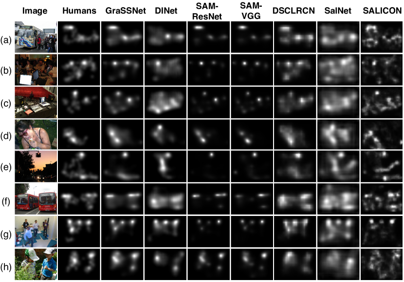
Figure 4: Qualitative comparison between our model and state-of-the-art saliency prediction methods. In each row, we list the image, ground truth, saliency maps without prior maps of our method and six state-of-the-arts models. Examples (a)-(e) demonstrate images with different object categories and examples (f)-(h) demonstrate images with the same object categories

4.4 Quantitative Analysis

As shown in Table 1, our method achieves state-of-the-art performances on all the datasets. It consistently outperforms other methods in all the metrics on SALICON. The promising results suggest that modeling semantic proximity is effective for improving the overall performance of saliency prediction. On the other datasets, GraSSNet also achieves better performances than the DINet that shares the same backbone as ours. Also, due to the differences in image characteristics among these datasets, the promising results demonstrate that the knowledge learned from the SALICON data can be successfully transferred to the other saliency datasets. It is noteworthy that GraSSNet includes CC and NSS as part of the objective, which gives advantages on CAT2000, MIT1003 and OSIE under both metrics. They complement each other and together ensure the model’s overall performance. The SIM scores of our model are also significantly better than the others even though SIM is not used as a training loss. Similarly, the KL scores are the best on SALICON, MIT1003, CAT2000 and the second-best on OSIE. Besides, our model also maintains improved sAUC values over DINet on SALICON when center bias is explicitly modeled.

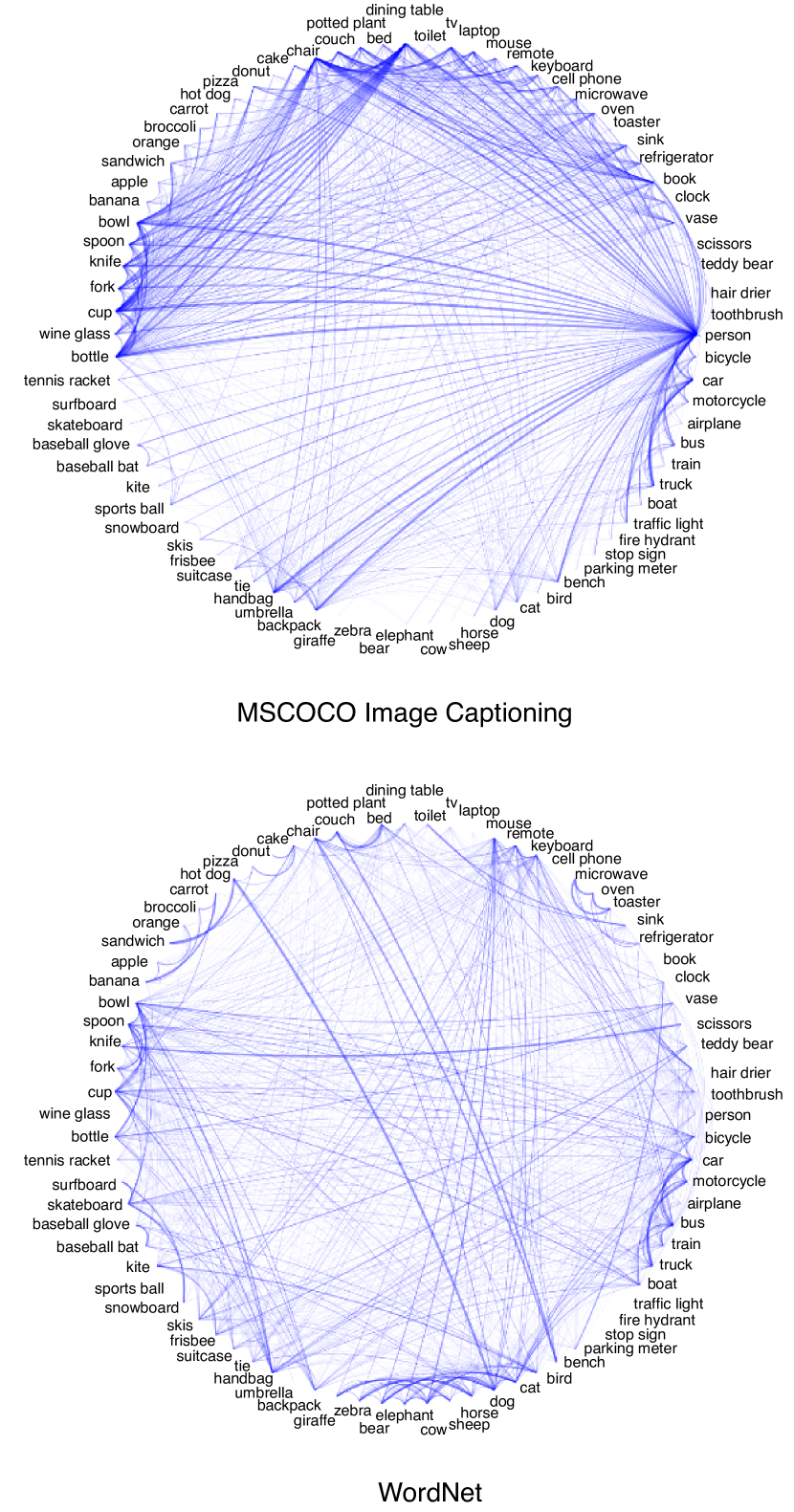
Figure 5: Visualization of external semantic proximity graphs. We visualize knowledge graph from MSCOCO image captioning (left) and WordNet (right) with classes as nodes in cycle layout. The width of the link indicates the strength of semantic proximity between the connected classes

4.5 Qualitative Analysis

We report the qualitative results of our model, in comparison with the state-of-the-art approaches. These qualitative examples are selected from the SALICON validation set, which demonstrates complex scenes in which semantic proximity can effectively improve saliency prediction. As shown in Fig. 4, our GraSSNet method performs the best for complex scenes with many objects in the foreground and background. In particular, for salient objects with strong semantic relationships, including both different objects (e.g. people and computers in Fig. 4c) and similar objects (e.g. multiple people in Fig. 4g), our method successfully predicts the relative saliency among these salient regions. To be more specific, taking Fig. 4a-d for example, our method captures the close relationship between the person and bus/computer/food, and hence highlights both. Similarly, both the traffic light and the car (Fig. 4e) get highlighted due to their strong semantic relationship. Besides, as can be seen from (Fig. 4f-h), which consists of multiple buses/people, the features are interchanged among them to intensify the saliency. A more detailed analysis of how regions are connected to produce proximity graph and how the distilled information benefits saliency prediction are discussed in Section 4.6.3.

4.6 Ablation Studies

To demonstrate the effectiveness of the various components and hyper-parameters used in the model, we conduct ablation studies on the SALICON dataset.

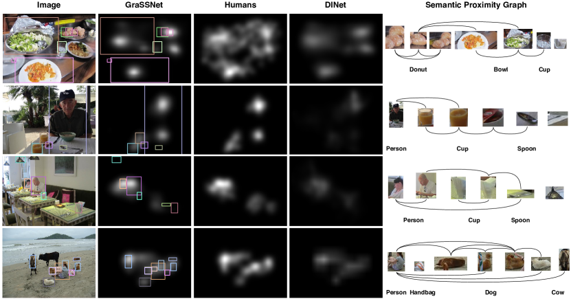
Figure 6: Visualization of region proposals and semantic proximity graphs. We show the proposed bounding boxes (the first column), saliency prediction results of our method without prior maps (the second column) and connected the regions with predicted edges from SPN (the last column). Besides, we list the ground truth fixation maps (the third column) and the saliency map of DINet (the fourth column)

Table 2: Ablation study of the external knowledge on the SALICON dataset. We test the performance of models without prior maps trained with different combinations of external knowledge for three different backbones (ResNet-50, ResNet-101 and VGG-19)

Backbone	External Knowledge	CC	AUC	NSS	sAUC
ResNet-50	-	0.851	0.874	3.239	0.762
ResNet-50	MSCOCO	0.863	0.886	3.251	0.784
ResNet-50	WordNet	0.861	0.884	3.247	0.778
ResNet-50	MSCOCO + WordNet	0.867	0.888	3.261	0.786
ResNet-101	-	0.841	0.864	3.084	0.757
ResNet-101	MSCOCO	0.861	0.887	3.252	0.777
ResNet-101	WordNet	0.859	0.879	3.234	0.761
ResNet-101	MSCOCO + WordNet	0.864	0.888	3.254	0.778
VGG-19	-	0.834	0.854	2.915	0.749
VGG-19	MSCOCO	0.855	0.882	3.246	0.775
VGG-19	WordNet	0.853	0.877	3.243	0.772
VGG-19	MSCOCO + WordNet	0.859	0.886	3.249	0.776

4.6.1 Effects of External Knowledge

We first examine how external knowledge benefits the saliency prediction. Table 2 reports the ablation study on the incorporation of external knowledge. On three different backbone networks, the comparison between models with and without external knowledge supervision shows that inclusion of external knowledge from MSCOCO image captioning and WordNet both improve the model performance. The results suggest that external knowledge about semantic proximity from both data sources can provide essential information for saliency prediction. Fig. 5 visualizes the semantic proximity graphs built from MSCOCO image captioning and WordNet, where nodes represent the 80 MSCOCO categories and the width of edges represents proximity. The figure illustrates that knowledge in MSCOCO is human-centric, providing a list of classes that commonly occur at the presence of the person type (e.g. handbag, spoon, cup, bowl, etc.). Besides, the knowledge graph from WordNet is relevant to the taxonomy of object types. It is quite effective in saliency prediction because objects of the same class are likely to appear together (e.g. knife, fork and spoon often present together as dinnerware). Taking multiple knowledge bases into account is helpful for the model’s generalizability to a broader domain.

4.6.2 Effects of Hyper-Parameters

Here we examine the choice of hyper-parameters. Firstly, since our loss function is a linear combination of $L_{1}$ distance, CC and NSS, as well as the MSE loss of edge predictions, we explore how different combinations of the parameters $\{\beta,\gamma,\lambda\}$ influence model performance. Results from Table 3 indicate that setting $\beta=0.3$, $\gamma=0.15$ and $\lambda=0.8$ can optimally balance the scores of different evaluation metrics and achieve the overall best performance.

Table 3: Ablation study of the hyper-parameters on the SALICON dataset. We report model performances without prior maps in four metrics (CC, AUC, NSS and sAUC) under different combinations of $\beta$, $\gamma$, $\lambda$

$\beta$	$\gamma$	$\lambda$	CC	AUC	NSS	sAUC
0.3	0.15	0.8	0.867	0.888	3.261	0.786
0.01	0.15	0.8	0.848	0.880	3.248	0.782
0.1	0.15	0.8	0.864	0.887	3.254	0.785
1	0.15	0.8	0.857	0.882	3.241	0.774
10	0.15	0.8	0.85	0.876	3.227	0.769
0.3	0.01	0.8	0.858	0.873	3.227	0.776
0.3	0.1	0.8	0.862	0.881	3.242	0.781
0.3	1	0.8	0.843	0.879	3.255	0.773
0.3	10	0.8	0.837	0.868	3.240	0.756
0.3	0.15	0.1	0.841	0.870	3.236	0.770
0.3	0.15	1	0.861	0.884	3.250	0.778
0.3	0.15	10	0.839	0.868	3.212	0.772

4.6.3 Visualizations

We visualize detected object regions and predicted semantic proximity graphs in Fig. 6, to illustrate the effects of semantic proximity information on saliency prediction. As can be seen, regions of the same category or related categories are interconnected with edges. Generally, edges are formed among all the donuts in Fig. 6a, most dogs in Fig. 6d, cups, spoons, and bowls in Fig. 6b. Such semantic proximity reflects the taxonomy of these words from the WordNet. Besides, some categories of objects are more related to people (e.g. handbag, cup, spoon, dog, etc.). This kind of human-centric semantic proximity is mostly derived from the MSCOCO image captioning. By taking into account the semantic proximity graphs, our model can better predict the saliency of semantically related regions.

5 Conclusion

In this paper, we present a novel saliency prediction network that explicitly models the semantic proximity as a graph, based on detected objects from the input. One of our key technical contributions is the novel SPN supervised by external knowledge. Beyond that, we proposed the sGAT to propagate the semantic information across the graph nodes, while preserving spatial features in node attributes. The modeling of semantic proximity allows our model to take the semantic relationships among multiple objects into account, and to better predict their relative saliency. The proposed method achieves promising performances on multiple saliency datasets. In future studies, we aim to extend this work by considering specific relationship modeling with the scene graph. We will also extend this work to video saliency and top-down saliency prediction.

References

- [1] Somak Aditya, Yezhou Yang, and Chitta Baral. Explicit reasoning over end-to-end neural architectures for visual question answering. In Thirty-Second AAAI Conference on Artificial Intelligence, 2018.
- [2] James Atwood and Don Towsley. Diffusion-convolutional neural networks. In Advances in Neural Information Processing Systems, pages 1993–2001, 2016.
- [3] Junwei Bao, Nan Duan, Ming Zhou, and Tiejun Zhao. Knowledge-based question answering as machine translation. In Proceedings of the 52nd Annual Meeting of the Association for Computational Linguistics (Volume 1: Long Papers), pages 967–976, 2014.
- [4] Neil DB Bruce, Christopher Catton, and Sasa Janjic. A deeper look at saliency: Feature contrast, semantics, and beyond. In Proceedings of the IEEE Conference on Computer Vision and Pattern Recognition, pages 516–524, 2016.
- [5] Joan Bruna, Wojciech Zaremba, Arthur Szlam, and Yann LeCun. Spectral networks and locally connected networks on graphs. arXiv preprint arXiv:1312.6203, 2013.
- [6] Zoya Bylinskii, Tilke Judd, Ali Borji, Laurent Itti, Frédo Durand, Aude Oliva, and Antonio Torralba. Mit saliency benchmark.
- [7] Zoya Bylinskii, Tilke Judd, Aude Oliva, Antonio Torralba, and Frédo Durand. What do different evaluation metrics tell us about saliency models? IEEE transactions on pattern analysis and machine intelligence, 41(3):740–757, 2018.
- [8] Chin-Kai Chang, Christian Siagian, and Laurent Itti. Mobile robot vision navigation & localization using gist and saliency. In 2010 IEEE/RSJ International Conference on Intelligent Robots and Systems, pages 4147–4154. IEEE, 2010.
- [9] Hans Colonius and Adele Diederich. Computing an optimal time window of audiovisual integration in focused attention tasks: illustrated by studies on effect of age and prior knowledge. Experimental Brain Research, 212(3):327–337, 2011.
- [10] Marcella Cornia, Lorenzo Baraldi, Giuseppe Serra, and Rita Cucchiara. Predicting human eye fixations via an lstm-based saliency attentive model. IEEE Transactions on Image Processing, 27(10):5142–5154, 2018.
- [11] Jia Deng, Nan Ding, Yangqing Jia, Andrea Frome, Kevin Murphy, Samy Bengio, Yuan Li, Hartmut Neven, and Hartwig Adam. Large-scale object classification using label relation graphs. In European conference on computer vision, pages 48–64. Springer, 2014.
- [12] David K Duvenaud, Dougal Maclaurin, Jorge Iparraguirre, Rafael Bombarell, Timothy Hirzel, Alán Aspuru-Guzik, and Ryan P Adams. Convolutional networks on graphs for learning molecular fingerprints. In Advances in neural information processing systems, pages 2224–2232, 2015.
- [13] Jiuxiang Gu, Handong Zhao, Zhe Lin, Sheng Li, Jianfei Cai, and Mingyang Ling. Scene graph generation with external knowledge and image reconstruction. In Proceedings of the IEEE Conference on Computer Vision and Pattern Recognition, pages 1969–1978, 2019.
- [14] Will Hamilton, Zhitao Ying, and Jure Leskovec. Inductive representation learning on large graphs. In Advances in Neural Information Processing Systems, pages 1024–1034, 2017.
- [15] Jonathan Harel, Christof Koch, and Pietro Perona. Graph-based visual saliency. In Advances in neural information processing systems, pages 545–552, 2007.
- [16] Mikael Henaff, Joan Bruna, and Yann LeCun. Deep convolutional networks on graph-structured data. arXiv preprint arXiv:1506.05163, 2015.
- [17] Geoffrey Hinton, Oriol Vinyals, and Jeff Dean. Distilling the knowledge in a neural network. arXiv preprint arXiv:1503.02531, 2015.
- [18] Xun Huang, Chengyao Shen, Xavier Boix, and Qi Zhao. Salicon: Reducing the semantic gap in saliency prediction by adapting deep neural networks. In Proceedings of the IEEE International Conference on Computer Vision, pages 262–270, 2015.
- [19] Katherine Humphrey and Geoffrey Underwood. Domain knowledge moderates the influence of visual saliency in scene recognition. British Journal of Psychology, 100(2):377–398, 2009.
- [20] Laurent Itti and Christof Koch. Computational modelling of visual attention. Nature reviews neuroscience, 2(3):194, 2001.
- [21] Sen Jia and Neil DB Bruce. Eml-net: An expandable multi-layer network for saliency prediction. Image and Vision Computing, page 103887, 2020.
- [22] Chenhan Jiang, Hang Xu, Xiaodan Liang, and Liang Lin. Hybrid knowledge routed modules for large-scale object detection. In Advances in Neural Information Processing Systems, pages 1552–1563, 2018.
- [23] Ming Jiang, Shengsheng Huang, Juanyong Duan, and Qi Zhao. Salicon: Saliency in context. In Proceedings of the IEEE conference on computer vision and pattern recognition, pages 1072–1080, 2015.
- [24] Ming Jiang and Qi Zhao. Learning visual attention to identify people with autism spectrum disorder. October 2017.
- [25] Tilke Judd, Krista Ehinger, Frédo Durand, and Antonio Torralba. Learning to predict where humans look. In 2009 IEEE 12th international conference on computer vision, pages 2106–2113. IEEE, 2009.
- [26] Diederik P Kingma and Jimmy Ba. Adam: A method for stochastic optimization. arXiv preprint arXiv:1412.6980, 2014.
- [27] Thomas N Kipf and Max Welling. Semi-supervised classification with graph convolutional networks. arXiv preprint arXiv:1609.02907, 2016.
- [28] Alex Krizhevsky, Ilya Sutskever, and Geoffrey E Hinton. Imagenet classification with deep convolutional neural networks. In Advances in neural information processing systems, pages 1097–1105, 2012.
- [29] Alexander Kroner, Mario Senden, Kurt Driessens, and Rainer Goebel. Contextual encoder-decoder network for visual saliency prediction. arXiv preprint arXiv:1902.06634, 2019.
- [30] Srinivas SS Kruthiventi, Kumar Ayush, and R Venkatesh Babu. Deepfix: A fully convolutional neural network for predicting human eye fixations. IEEE Transactions on Image Processing, 26(9):4446–4456, 2017.
- [31] Srinivas SS Kruthiventi, Vennela Gudisa, Jaley H Dholakiya, and R Venkatesh Babu. Saliency unified: A deep architecture for simultaneous eye fixation prediction and salient object segmentation. In Proceedings of the IEEE Conference on Computer Vision and Pattern Recognition, pages 5781–5790, 2016.
- [32] Matthias Kümmerer, Lucas Theis, and Matthias Bethge. Deep gaze i: Boosting saliency prediction with feature maps trained on imagenet. arXiv preprint arXiv:1411.1045, 2014.
- [33] Olivier Le Meur and Patrick Le Callet. What we see is most likely to be what matters: Visual attention and applications. In 2009 16th IEEE International Conference on Image Processing (ICIP), pages 3085–3088. IEEE, 2009.
- [34] Guohao Li, Hang Su, and Wenwu Zhu. Incorporating external knowledge to answer open-domain visual questions with dynamic memory networks. arXiv preprint arXiv:1712.00733, 2017.
- [35] Tsung-Yi Lin, Michael Maire, Serge Belongie, James Hays, Pietro Perona, Deva Ramanan, Piotr Dollár, and C Lawrence Zitnick. Microsoft coco: Common objects in context. In European conference on computer vision, pages 740–755. Springer, 2014.
- [36] Nian Liu and Junwei Han. A deep spatial contextual long-term recurrent convolutional network for saliency detection. IEEE Transactions on Image Processing, 27(7):3264–3274, 2018.
- [37] Matei Mancas, Nicolas Riche, Julien Leroy, and Bernard Gosselin. Abnormal motion selection in crowds using bottom-up saliency. In 2011 18th IEEE International Conference on Image Processing, pages 229–232. IEEE, 2011.
- [38] George A Miller. Wordnet: a lexical database for english. Communications of the ACM, 38(11):39–41, 1995.
- [39] Tam V Nguyen, Qi Zhao, and Shuicheng Yan. Attentive systems: A survey. International Journal of Computer Vision, 126(1):86–110, 2018.
- [40] Junting Pan, Elisa Sayrol, Xavier Giro-i Nieto, Kevin McGuinness, and Noel E O’Connor. Shallow and deep convolutional networks for saliency prediction. In Proceedings of the IEEE Conference on Computer Vision and Pattern Recognition, pages 598–606, 2016.
- [41] Robert J Peters, Asha Iyer, Laurent Itti, and Christof Koch. Components of bottom-up gaze allocation in natural images. Vision research, 45(18):2397–2416, 2005.
- [42] Shaoqing Ren, Kaiming He, Ross Girshick, and Jian Sun. Faster r-cnn: Towards real-time object detection with region proposal networks. In Advances in neural information processing systems, pages 91–99, 2015.
- [43] Nicolas Riche, Matthieu Duvinage, Matei Mancas, Bernard Gosselin, and Thierry Dutoit. Saliency and human fixations: State-of-the-art and study of comparison metrics. In Proceedings of the IEEE international conference on computer vision, pages 1153–1160, 2013.
- [44] Christian Szegedy, Wei Liu, Yangqing Jia, Pierre Sermanet, Scott Reed, Dragomir Anguelov, Dumitru Erhan, Vincent Vanhoucke, and Andrew Rabinovich. Going deeper with convolutions. In Proceedings of the IEEE conference on computer vision and pattern recognition, pages 1–9, 2015.
- [45] Benjamin W Tatler. The central fixation bias in scene viewing: Selecting an optimal viewing position independently of motor biases and image feature distributions. Journal of vision, 7(14):4–4, 2007.
- [46] Petar Veličković, Guillem Cucurull, Arantxa Casanova, Adriana Romero, Pietro Lio, and Yoshua Bengio. Graph attention networks. arXiv preprint arXiv:1710.10903, 2017.
- [47] Eleonora Vig, Michael Dorr, and David Cox. Large-scale optimization of hierarchical features for saliency prediction in natural images. In Proceedings of the IEEE Conference on Computer Vision and Pattern Recognition, pages 2798–2805, 2014.
- [48] Shuo Wang, Shaojing Fan, Bo Chen, Shabnam Hakimi, Lynn K Paul, Qi Zhao, and Ralph Adolphs. Revealing the world of autism through the lens of a camera. Current Biology, 26(20):R909–R910, 2016.
- [49] Wenguan Wang, Jianbing Shen, and Fatih Porikli. Saliency-aware geodesic video object segmentation. In Proceedings of the IEEE conference on computer vision and pattern recognition, pages 3395–3402, 2015.
- [50] Zhibiao Wu and Martha Palmer. Verbs semantics and lexical selection. In Proceedings of the 32nd annual meeting on Association for Computational Linguistics, pages 133–138. Association for Computational Linguistics, 1994.
- [51] Juan Xu, Ming Jiang, Shuo Wang, Mohan S Kankanhalli, and Qi Zhao. Predicting human gaze beyond pixels. Journal of vision, 14(1):28–28, 2014.
- [52] Sheng Yang, Guosheng Lin, Qiuping Jiang, and Weisi Lin. A dilated inception network for visual saliency prediction. arXiv preprint arXiv:1904.03571, 2019.
- [53] Ruichi Yu, Ang Li, Vlad I Morariu, and Larry S Davis. Visual relationship detection with internal and external linguistic knowledge distillation. In Proceedings of the IEEE international conference on computer vision, pages 1974–1982, 2017.
- [54] Lingyun Zhang, Matthew H Tong, Tim K Marks, Honghao Shan, and Garrison W Cottrell. Sun: A bayesian framework for saliency using natural statistics. Journal of vision, 8(7):32–32, 2008.
- [55] Wei Zhang, Ali Borji, Zhou Wang, Patrick Le Callet, and Hantao Liu. The application of visual saliency models in objective image quality assessment: A statistical evaluation. IEEE transactions on neural networks and learning systems, 27(6):1266–1278, 2015.