A critical quartet for queuing couples

Abstract

We enumerate arrangements of $n$ couples, i.e. pairs of people, placed in a single-file queue, and consider four statistics from the vantage point of a distinguished given couple. In how many arrangements are exactly $p$ of the $n-1$ other couples i) interlaced with the given couple, ii) contained within them, iii) containing the given couple, and iv) lying outside the given couple? We provide generating functions which enumerate these arrangements and obtain the associated continuous asymptotic distributions in the $n\to\infty$ limit. The asymptotic distributions corresponding to cases i), iii), and iv) evince critical phenomena around the value $p_{c}=(n-1)/2$, such that the probability that 1) the couple is interlaced with more than half of the other couples, and 2) the couple is contained by more than half of the other couples, are both zero in the strict $n\to\infty$ limit. We further show that the cumulative probability that less than half of the other couples lie outside the given couple is $\pi/4$ in the limit, and that the associated distribution is uniform for $p<p_{c}$ .

1 Introduction and main results

The purpose of this paper is to study linear arrangements of $n$ distinguishable pairs of objects, treating the two members of a pair as indistinguishable. The connection to linear chord diagrams is immediate, as we can represent the pairs as chords joining two of $2n$ vertices laid out in a line, see Figure 1. The main difference is that we treat the $n$ chords, ab initio, as distinguishable.

The study of (indistinguishable) chord diagrams has a rich history. Touchard [9] and Riordan [6] enumerated configurations by the total number of crossings, and the limiting Normal distribution was obtained by Flajolet and Noy [2]. More recently Pilaud and Rué [5] have extended the study of crossings in several directions. Kreweras and Poupard [4] enumerated configurations by the number of so-called short pairs, where adjacent vertices are joined by a chord, finding that they are asymptotically Poisson in distribution; c.f. Cameron and Killpatrick [1] and Krasko and Omelchenko [3] for more modern treatments.

We will enumerate configurations from the vantage point of a distinguished given pair (which might appear in any position) according to the relative position of the remaining $n-1$ pairs. Each of these remaining pairs can be in one of four relative positions: i) interlaced with the given pair, ii) entirely contained within the endpoints of the given pair, iii) arching over the given pair and hence entirely containing it, or iv) positioned entirely outside, either to the left, or to the right, of the given pair.

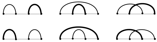
Figure 1: The 6 configurations for the case $n=2$. The given pair is indicated as a bold arc. There are 4 configurations where the given pair is not crossed, hence $K_{2,0}=4$, whilst there are 2 where it is crossed once, hence $K_{2,1}=2$. Similarly $C_{2,0}=G_{2,0}=5$, $C_{2,1}=G_{2,1}=1$, and $X_{2,0}=4$, $X_{2,1}=2$.

It is clear that the total number of arrangements of the $n$ distinguishable pairs is $n!\,(2n-1)!!$, as there are $(2n-1)!!$ different linear chord diagrams. Due to the fact that we are essentially interested in a single marked pair, i.e. the given pair, we can safely paint the remaining $n-1$ pairs with the same brush and treat them as indistinguishable – this yields $n\,(2n-1)!!$ configurations, and is the number of linear chord diagrams with one marked chord.

Definition 1.

A pair is said to be crossed by another pair if the other pair has one endpoint contained within the first pair, and the other outside of it, i.e. the two pairs are interlaced.

Definition 2.

A pair is said to be contained by another pair if its endpoints are both located within the endpoints of the other pair.

Definition 3.

A pair is said to be containing another pair if the other pair is contained by it.

Definition 4.

A pair is said to be excluded by another pair if its endpoints are both to the left, or both to the right of the other pair.

Amongst the $n\,(2n-1)!!$ arrangements, let there be $K_{n,p}$ where exactly $p\in[0,n-1]$ of the remaining $n-1$ pairs are crossed by the given pair. Similarly we define $C_{n,p}$, $G_{n,p}$, and $X_{n,p}$ to be the number of configurations where exactly $p$ of the remaining pairs are, respectively, contained by, containing, and finally excluded by the given pair; see Figure 1.

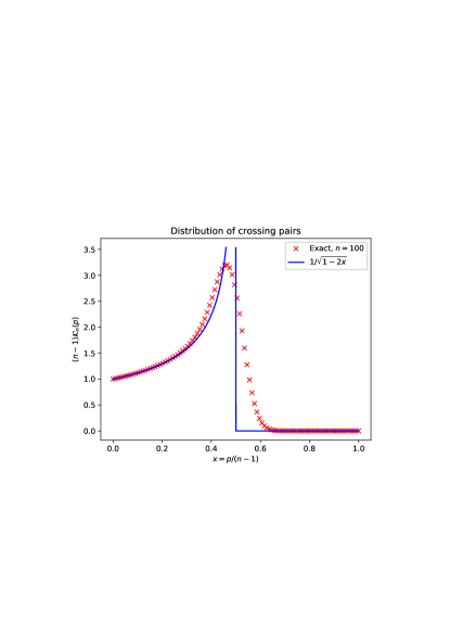
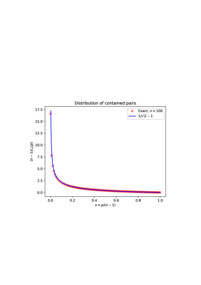
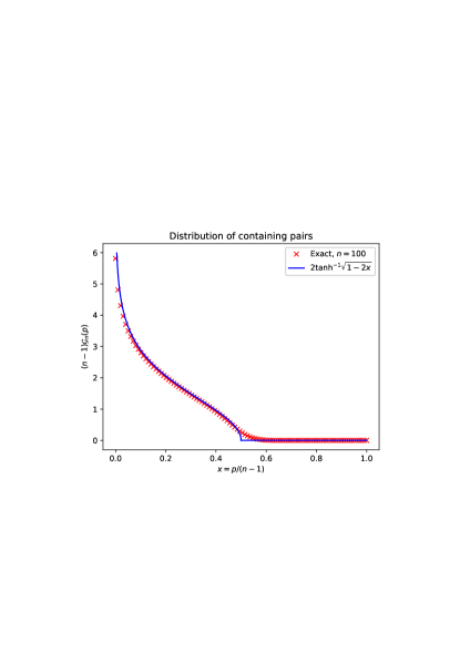
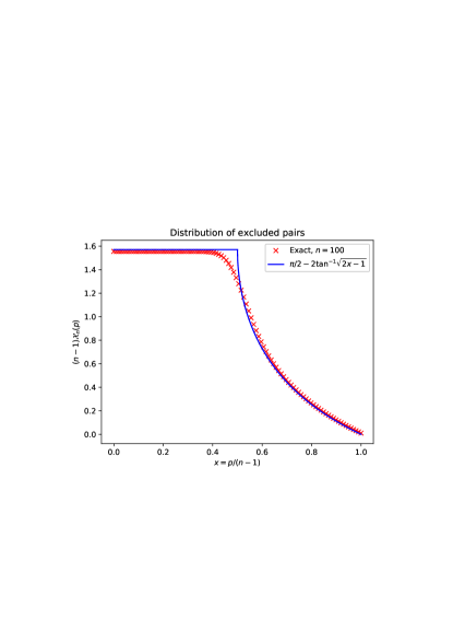
Figure 2: The quartet of distributions. On the top row: on the left the distribution of pairs crossing the given pair, on the right pairs contained within the given pair. On the bottom row: on the left pairs which contain the given pair, on the right pairs situated outside the given pair. In each case the solid blue line is the asymptotic distribution, while the red “x” is the discrete value from the exact distribution for $n=100$.

Generating functions We define exponential generating functions as follows

$$K(y,z)=\sum_{n\geq 1}\sum_{p=0}^{n-1}K_{n,p}\,y^{p}\,\frac{z^{n}}{n!},$$

and similarly for the $C_{n,p}\to C(y,z)$, $G_{n,p}\to G(y,z)$, and $X_{n,p}\to X(y,z)$. In Theorems 8, 13, 18, and 24 we prove that

$$\begin{split}&K(y,z)=\frac{z}{\sqrt{1-2z}\left(1-z(1+y)\right)},\quad C(y,z)=\frac{\sqrt{1-2yz}-\sqrt{1-2z}}{(1-2z)(1-y)},\\ &G(y,z)=\frac{1}{(1-y)\sqrt{1-2z}}\ln\left(\frac{1-z(1+y)}{1-2z}\right),\\ &X(y,z)=\frac{1}{(1-y)\sqrt{1-2z}}\tan^{-1}\frac{(1-y)z}{\sqrt{(1-2z)(1-2yz)}}.\end{split}$$

The form of $K(y,z)$ implies the recursion relation $K_{n,p}=n\,K_{n-1,p}+n\,K_{n-1,p-1}$, $K_{n,0}=[z^{n}]K(0,z)$.

Asymptotic distributions We will also be interested in the associated discrete probability distributions

$$P(\text{exactly $p$ pairs cross the given pair})={\cal K}_{n}(p)=\frac{1}{n\,(2n-1)!!}\,K_{n,p},$$

and so for ${\cal C}_{n}(p)$, ${\cal G}_{n}(p)$, and ${\cal X}_{n}(p)$, where we treat all $n\,(2n-1)!!$ arrangements as equally likely. In the limit as $n\to\infty$ we define a continuous real variable $x=\lim_{n\to\infty}p/(n-1)\in[0,1]$, and an associated continuous probability distribution

$${\cal K}(x)=\lim_{n\to\infty}(n-1)\,{\cal K}_{n}\left((n-1)x\right),$$

and so for ${\cal C}(x)$, ${\cal G}(x)$, and ${\cal X}(x)$. In Theorems 11, 15, 21, and 26 we prove that

$$\begin{split}&{\cal K}(x)=\begin{cases}1/\sqrt{1-2x}&0\leq x<1/2\\ 0&1/2\leq x\leq 1\end{cases},\qquad{\cal C}(x)=\frac{1}{\sqrt{x}}-1,\quad 0<x\leq 1,\\ &{\cal G}(x)=\begin{cases}2\tanh^{-1}\sqrt{1-2x}&0<x\leq 1/2\\ 0&1/2<x\leq 1\end{cases},\\ &{\cal X}(x)=\begin{cases}\pi/2&0\leq x<1/2\\ \pi/2-2\tan^{-1}\sqrt{2x-1}&1/2\leq x\leq 1\end{cases}.\end{split}$$

In Figure 2 the four distributions are shown. It is remarkable that ${\cal K}(x)$, ${\cal G}(x)$, and ${\cal X}(x)$ all show critical phenomena at $x=1/2$, corresponding to half of the $n-1$ pairs. This is most striking in the discontinuity observed in ${\cal K}(x)$, where the asymptotic probability that the given pair is crossed by more than half of the remaining pairs is zero, while the mode of the distribution is also half of the remaining pairs. In ${\cal G}(x)$ we see that the asymptotic probability that the given pair is contained within more than half of the remaining pairs is also zero. The distribution ${\cal X}(x)$ shows that the asymptotic (cumulative) probability that less than half of the remaining pairs are outside the given pair is given by $\pi/4$, while the distribution itself is uniform in this region.

In Lemmas 10, 14, 19, and 25, we obtain expressions for the $m^{\text{th}}$ factorial moments of the exact distributions. In particular,

$$\begin{split}&\sum_{p=0}^{n-1}\frac{p!}{(p-m)!}\,{\cal K}_{n}(p)=\frac{(n-1)!}{(n-m-1)!}\frac{m!}{(2m+1)!!},\\ &\sum_{p=0}^{n-1}\frac{p!}{(p-m)!}\,{\cal C}_{n}(p)=\frac{(n-1)!}{(n-m-1)!}\frac{1}{(m+1)(2m+1)},\\ &\sum_{p=0}^{n-1}\frac{p!}{(p-m)!}\,{\cal G}_{n}(p)=\frac{(n-1)!}{(n-m-1)!}\frac{m!}{(m+1)(2m+1)!!},\\ &\sum_{p=0}^{n-1}\frac{p!}{(p-m)!}\,{\cal X}_{n}(p)=\frac{(n-1)!}{(n-m-1)!}\frac{1}{m+1}\int_{1/2}^{1}dx\,\frac{x^{m}}{\sqrt{2x-1}}.\end{split}$$

The mean values for the four distributions tell us that, on average, a third of the remaining pairs cross the given pair, a sixth are contained by it, another sixth contain the given pair, and the remaining third are excluded by it.

2 Enumeration by crossings

Definition 5.

We define the size of a pair to be the number of vertices contained between its endpoints; the minimum size is zero, while the maximum size achievable is $2n-2$.

Distribution of sizes There are clearly $(2n-d-1)$ positions a given pair of size $d$ can occupy. Once placed, there are $(2n-3)!!$ ways of placing the remaining $(n-1)$ indistinguishable pairs. The probability ${\cal S}_{n}(d)$ that the given pair has size $d$ is therefore

$${\cal S}_{n}(d)=(2n-d-1)\frac{(2n-3)!!}{n\,(2n-1)!!}=\frac{1}{n}\left(1-\frac{d}{2n-1}\right),$$

which is a trapezoidal distribution. Straightforward computations yield a mean of $2(n-1)/3$, or a third of the maximal distance, and a variance of $(2n+1)(n-1)/9$.

Counting by crossings The minimum number of times a given pair can be crossed is zero – this is when all its contained vertices are matched amongst one another, and so with all its excluded vertices. The maximum number of times a given pair can be crossed is $n-1$ as there are $2n-2$ vertices other than those occupied by the endpoints of the given pair, and to achieve the maximal crossing we require half of them to be contained (i.e. the given pair has a size of $n-1$) and then each matched with one of the $n-1$ excluded vertices. Let $p$ be the number of times a given pair of size $d$ is crossed. It is clear that $p\equiv d\pmod{2}$.

Proposition 6.

The number $K_{n,p,d}$ of configurations in which the given pair has size $d$, and is crossed by $p$ other pairs, is given by

$$K_{n,p,d}=\frac{2^{p-n+1}\,d!\,(2n-d-1)!}{p!\,\left(n-1-\frac{d-p}{2}\right)!\,\left(\frac{d-p}{2}\right)!},$$

where $d\,\mathrm{mod}\,2\leq p\leq\min(d,2n-d-2)$, and $0\leq d\leq 2n-2$.

Proof.

In order to enumerate configurations where a given pair of size $d$ is crossed $p$ times, we consider the $d$ contained vertices, and choose $p$ of these to be matched with another selection of $p$ excluded vertices. The remaining contained vertices are then matched amongst themselves, and so for the remaining excluded vertices.

• There are $p!{d\choose p}{2n-d-2\choose p}$ ways of choosing the $p$ contained and $p$ excluded vertices and then matching them up.

• There are $(d-p-1)!!\,(2n-d-p-3)!!$ ways of matching the remaining vertices.

• There are $(2n-d-1)$ positions for the given pair to occupy.

We therefore have that

$$K_{n,d,p}={d\choose p}{2n-d-2\choose p}\,p!\,(d-p-1)!!\,(2n-d-p-3)!!\,(2n-d-1).$$

Using the identity $(2n-1)!!=(2n)!/(n!2^{n})$, and simplifying this expression, we obtain the desired result. ∎

$n$ \$p$	0	1	2	3	4	5
1	1
2	4	2
3	21	18	6
4	144	156	96	24
5	1245	1500	1260	600	120
6	13140	16470	16560	11160	4320	720

Table 1: The numbers $K_{n,p}$, A336598 in the OEIS, to appear. The first column is A233481. The leading diagonal are the factorials $n!$.

Lemma 7.

The number $K_{n,p}$ of configurations in which the given pair is crossed by $p$ other pairs, is given by

$$K_{n,p}=n\,(2n-1)!!\int_{0}^{1}d\alpha\,2(1-\alpha)\,{n-1\choose p}\left(2\alpha(1-\alpha)\right)^{p}\left(1-2\alpha(1-\alpha)\right)^{n-p-1}.$$

Proof.

We sum the result of Proposition 6 over sizes $d$ to produce $K_{n,p}$. For fixed $p$, we must sum $d$ over the range $p\leq d\leq 2n-2-p$, where $d$ is incremented by $2$ in each successive term. To make this summation more convenient we write $d=2k+p$ and sum $k$ over $0\leq k\leq n-p-1$:

$$K_{n,p}=\frac{2^{p-n+1}}{p!}\sum_{k=0}^{n-p-1}\frac{(2k+p)!\,(2n-2k-p-1)!}{(n-p-k-1)!\,k!}.$$

We now exploit the following integral representation of the Euler Beta function:

$$\frac{(2k+p)!\,(2n-2k-p-1)!}{(2n)!}=\int_{0}^{1}d\alpha\,\alpha^{2k+p}\,(1-\alpha)^{2n-2k-p-1},$$

to obtain

$$\begin{split}K_{n,p}&=\frac{2^{p-n+1}\,(2n)!}{p!}\int_{0}^{1}d\alpha\,\sum_{k=0}^{n-p-1}\frac{\alpha^{2k+p}\,(1-\alpha)^{2n-2k-p-1}}{(n-k-p-1)!\,k!}\\ &=\frac{2^{p-n+1}\,(2n)!}{p!}\int_{0}^{1}d\alpha\,\sum_{k=0}^{n-p-1}\frac{\alpha^{p}\,(1-\alpha)^{2n-p-1}}{(n-k-p-1)!\,k!}\,\left(\frac{\alpha^{2}}{(1-\alpha)^{2}}\right)^{k}\\ &=\frac{2^{p-n+1}\,(2n)!}{p!}\int_{0}^{1}d\alpha\,\frac{\alpha^{p}\,(1-\alpha)^{2n-p-1}}{(n-p-1)!}\,\left(1+\frac{\alpha^{2}}{(1-\alpha)^{2}}\right)^{n-p-1}\\ &=n\,(2n-1)!!\,{n-1\choose p}\int_{0}^{1}d\alpha\,2(1-\alpha)\,\left(2\alpha(1-\alpha)\right)^{p}\left((1-\alpha)^{2}+\alpha^{2}\right)^{n-p-1}\\ &=n\,(2n-1)!!\int_{0}^{1}d\alpha\,2(1-\alpha)\,{n-1\choose p}\left(2\alpha(1-\alpha)\right)^{p}\left(1-2\alpha(1-\alpha)\right)^{n-p-1}.\end{split}$$

∎

Theorem 8.

The exponential generating function $K(y,z)$ is given by

$$K(y,z)=\sum_{n\geq 1}\sum_{p=0}^{n-1}K_{n,p}\,y^{p}\,\frac{z^{n}}{n!}=\frac{z}{\sqrt{1-2z}\left(1-z(1+y)\right)}.$$

Proof.

We sum the result of Lemma 7 against $y^{p}$ to obtain

$$\sum_{p=0}^{n-1}K_{n,p}\,y^{p}=n\,(2n-1)!!\int_{0}^{1}d\alpha\,2(1-\alpha)\,\bigl{(}1-(1-y)2\alpha(1-\alpha)\bigr{)}^{n-1}.$$

We then perform the sum over $n$ against $z^{n}/n!$

$$\begin{split}&\sum_{n,p}K_{n,p}\,y^{p}\,\frac{z^{n}}{n!}=\sum_{n}\frac{n\,(2n-1)!!}{n!}\,z^{n}\int_{0}^{1}d\alpha\,2(1-\alpha)\,\bigl{(}1-(1-y)2\alpha(1-\alpha)\bigr{)}^{n-1}\\ &=\int_{0}^{1}d\alpha\,2(1-\alpha)\frac{z}{\left(1-2z\left(1-(1-y)2\alpha(1-\alpha)\right)\right)^{3/2}}=\frac{z}{\sqrt{1-2z}\left(1-z(1+y)\right)}.\end{split}$$

∎

Corollary 9.

The $K_{n,p}$ obey the following recursion relation

$$K_{n,p}=n\,K_{n-1,p}+n\,K_{n-1,p-1},\qquad K_{n,0}=[z^{n}]\frac{z}{\sqrt{1-2z}\left(1-z\right)},$$

where we note that $K_{n,0}$ is $\href http://oeis.org/A233481$ in the OEIS – the number of singletons (strong fixed points) in pair-partitions.

Proof.

The recursion relation is implied by the factor $1-z(1+y)$ in the denominator of the generating function $K(y,z)$. ∎

Probability distribution and asymptotics

We define a discrete random variable $K$ which corresponds to the number of pairs which cross the given pair. The result of Lemma 7 implies that the probability that $K$ takes the value $p$ is given by

$${\cal K}_{n}(p)=\frac{K_{n,p}}{n\,(2n-1)!!}=\int_{0}^{1}d\alpha\,2(1-\alpha)\,{n-1\choose p}\left(2\alpha(1-\alpha)\right)^{p}\left(1-2\alpha(1-\alpha)\right)^{n-p-1},$$

which is an integral over Binomial distributions. In order to compute the factorial moments of this distribution, we define a generating function as follows

$${\cal P}_{n}(y)=\sum_{p=0}^{n-1}{\cal K}_{n}(p)\,y^{p}=\int_{0}^{1}d\alpha\,2(1-\alpha)\,\bigl{(}1-(1-y)2\alpha(1-\alpha)\bigr{)}^{n-1}.$$

Lemma 10.

The $m^{\text{th}}$ factorial moment of ${\cal K}_{n}(p)$ is given by

$$\sum_{p=0}^{n-1}\frac{p!}{(p-m)!}\,{\cal K}_{n}(p)=\frac{(n-1)!}{(n-m-1)!}\frac{m!}{(2m+1)!!}.$$

In particular this provides the mean $E(K)=(n-1)/3$, and the variance $\mathrm{Var}(K)=(n-1)(n+8)/45$.

Proof.

$$\begin{split}&\sum_{p=0}^{n-1}\frac{p!}{(p-m)!}\,{\cal K}_{n}(p)=\left.\frac{d^{m}}{dy^{m}}\right|_{y=1}{\cal P}_{n}(y)=\int_{0}^{1}d\alpha\,2(1-\alpha)\,\frac{(n-1)!}{(n-m-1)!}\left(2\alpha(1-\alpha)\right)^{m}\\ &=2^{m+1}\frac{(n-1)!}{(n-m-1)!}\frac{m!\,(m+1)!}{(2m+2)!}=\frac{(n-1)!}{(n-m-1)!}\frac{m!}{(2m+1)!!}.\end{split}$$

∎

In the limit as $n\to\infty$ we define a continuous real variable $x=\lim_{n\to\infty}p/(n-1)\in[0,1]$, and an associated continuous probability distribution

$${\cal K}(x)=\lim_{n\to\infty}(n-1)\,{\cal K}_{n}\left((n-1)x\right),$$

Theorem 11.

The asymptotic distribution ${\cal K}(x)$ is given by

$${\cal K}(x)=\begin{cases}1/\sqrt{1-2x}&0\leq x<1/2\\ 0&1/2\leq x\leq 1\end{cases}.$$

Proof.

The most satisfying proof of this fact is to show that the large-$n$ limit of the factorial moments is correctly reproduced. To wit,

$$\int_{0}^{1/2}dx\,\frac{x^{m}}{\sqrt{1-2x}}=\frac{1}{2^{m+1}}\int_{0}^{1}du\,u^{-1/2}(1-u)^{m}=\frac{m!}{(2m+1)!!},$$

where we have used the substitution $u=1-2x$. Comparing to Lemma (10), we see that in the large-$n$ limit $\frac{(n-1)!}{(n-m-1)!}\to n^{m}$, and so we are indeed recovering the factorial moments correctly. ∎

Alternative proof Another perspective is to return to the following representation of the exact distribution

$$\int_{0}^{1}d\alpha\,2(1-\alpha)\,{n-1\choose p}\left(2\alpha(1-\alpha)\right)^{p}\left(1-2\alpha(1-\alpha)\right)^{n-p-1},$$

and to use the Normal approximation of the Binomial distribution. When $\alpha$ is near 0 or 1, this will not be a good approximation, but this seems to be a set of small enough measure not to impact the overall approximation for $n\to\infty$. We begin by changing the integration variable $\alpha=\sin^{2}{\theta\over 2}$

$$\int_{0}^{\pi}d\theta\,\sin\theta\,\frac{1+\cos\theta}{2}\,{n-1\choose p}\left(\frac{\sin^{2}\theta}{2}\right)^{p}\left(\frac{1+\cos^{2}\theta}{2}\right)^{n-p-1},$$

where we note that $1+\cos\theta$ may be replaced by $1$ as the rest of the integrand is even about $\theta=\pi/2$. We now take an integral over Normal distributions with mean ${1\over 2}(n-1)\sin^{2}\theta$ and variance ${1\over 4}(n-1)\sin^{2}\theta\left(1+\cos^{2}\theta\right)={1\over 4}(n-1)\left(1-\cos^{4}\theta\right)$

$$N(x)=\frac{\sqrt{n-1}}{\sqrt{2\pi}}\int_{0}^{\pi}\frac{d\theta}{\sqrt{1+\cos^{2}\theta}}\,\mathrm{Exp}\left(\frac{-2\,(n-1)\left(x-{1\over 2}\sin^{2}\theta\right)^{2}}{1-\cos^{4}\theta}\right).$$

This distribution interpolates between the discrete values of the actual distribution remarkably well, and the integral over $\theta$ converges well enough to allow for efficient numerical integration for all values of $x$. It has a tail for $x<0$ which is suppressed for large $n$. It is straightforward to show that all the moments match the actual distribution in the strict $n\to\infty$ limit; $N(x)$ also has the exact mean and variance, and the third moment is correct at ${\cal O}(n^{-1})$. Taking the $n\to\infty$ limit, we may use the method of steepest descent to evaluate the integral. For $x\in[0,1/2)$, there are two saddle points located at the following values of $\theta$

$$\theta_{0}=\arcsin\sqrt{2x},\qquad\theta_{1}=\pi-\arcsin\sqrt{2x},$$

which yield the dominant contributions to the integral. Representing $N(x)$ as

$$\int d\theta\,f(\theta)\,e^{(n-1)S(\theta)},$$

one finds that

$$\left.\frac{d^{2}S}{d\theta^{2}}\right|_{\theta=\theta_{0}}=\left.\frac{d^{2}S}{d\theta^{2}}\right|_{\theta=\theta_{1}}=-\frac{4\cos^{2}\theta_{0}}{1+\cos^{2}\theta_{0}},$$

and so the two saddle points contribute the same result, namely

$$\begin{split}&\frac{\sqrt{2\pi}}{\sqrt{n-1}}\,f(\theta_{0})\,\left(-\left.\frac{d^{2}S}{d\theta^{2}}\right|_{\theta=\theta_{0}}\right)^{-1/2}=\frac{\sqrt{2\pi}}{\sqrt{n-1}}\,f(\theta_{1})\,\left(-\left.\frac{d^{2}S}{d\theta^{2}}\right|_{\theta=\theta_{1}}\right)^{-1/2}\\ &=\frac{1}{2|\cos\theta_{0}|}=\frac{1}{2|\cos\theta_{1}|}=\frac{1}{2}\frac{1}{\sqrt{1-2x}},\end{split}$$

and so the sum of the two contributions yields the desired result.

3 Enumeration by contained pairs

We now enumerate configurations according to the number $p$ of pairs contained within the given pair. We begin by summing the result of Proposition 6 over all possible crossings, noting that if a contained vertex is not part of a crossing pair, it is necessarily part of a contained pair. We let $d=2p+k$, so that the number of crossings $k$ is bounded between $0\leq k\leq n-p-1$.

Lemma 12.

The number $C_{n,p}$ of configurations in which the given pair contains $p$ other pairs, is given by

$$C_{n,p}=\sum_{k=0}^{n-p-1}K_{n,k,2p+k}=n\,(2n-1)!!\int_{0}^{1}d\alpha\,2(1-\alpha){n-1\choose p}\left(\alpha^{2}\right)^{p}\left(1-\alpha^{2}\right)^{n-1-p}.$$

Proof.

We exploit the Euler Beta integral used in the proof of Lemma 7.

$$\begin{split}C_{n,p}&=\frac{2^{k-n+1}\,(2n)!}{p!}\int_{0}^{1}d\alpha\,\sum_{k=0}^{n-p-1}\frac{\alpha^{2p+k}\,(1-\alpha)^{2n-2p-k-1}}{(n-k-p-1)!\,k!}\\ &=\frac{2^{-n+1}\,(2n)!}{p!}\int_{0}^{1}d\alpha\,\sum_{k=0}^{n-p-1}\frac{\alpha^{2p}\,(1-\alpha)^{2n-2p-1}}{(n-k-p-1)!\,k!}\,\left(\frac{2\alpha}{1-\alpha}\right)^{k}\\ &=n\,(2n-1)!!\,{n-1\choose p}\int_{0}^{1}d\alpha\,2(1-\alpha)\,\alpha^{2p}(1-\alpha)^{n-p}\left(1+\alpha\right)^{n-p-1}\\ &=n\,(2n-1)!!\int_{0}^{1}d\alpha\,2(1-\alpha){n-1\choose p}\left(\alpha^{2}\right)^{p}\left(1-\alpha^{2}\right)^{n-1-p}.\end{split}$$

∎

Theorem 13.

The exponential generating function $C(y,z)$ is given by

$$C(y,z)=\sum_{n\geq 1}\sum_{p=0}^{n-1}C_{n,p}\,y^{p}\,\frac{z^{n}}{n!}=\frac{\sqrt{1-2yz}-\sqrt{1-2z}}{(1-2z)(1-y)}.$$

Proof.

We sum the result of Lemma 12 against $y^{p}$ to obtain

$$\sum_{p=0}^{n-1}C_{n,p}\,y^{p}=n\,(2n-1)!!\int_{0}^{1}d\alpha\,2(1-\alpha)\,\bigl{(}1-(1-y)\alpha^{2}\bigr{)}^{n-1}.$$

We then perform the sum over $n$ against $z^{n}/n!$

$$\begin{split}&\sum_{n,p}C_{n,p}\,y^{p}\,\frac{z^{n}}{n!}=\sum_{n}\frac{n\,(2n-1)!!}{n!}\,z^{n}\int_{0}^{1}d\alpha\,2(1-\alpha)\,\bigl{(}1-(1-y)\alpha^{2}\bigr{)}^{n-1}\\ &=\int_{0}^{1}d\alpha\,2(1-\alpha)\frac{z}{\left(1-2z\left(1-(1-y)\alpha^{2}\right)\right)^{3/2}}=\frac{\sqrt{1-2yz}-\sqrt{1-2z}}{(1-2z)(1-y)}.\end{split}$$

∎

$n$ \$p$	0	1	2	3	4	5
1	1
2	5	1
3	33	9	3
4	279	87	39	15
5	2895	975	495	255	105
6	35685	12645	6885	4005	2205	945

Table 2: The numbers $C_{n,p}$, A336599 in the OEIS, to appear. The leading diagonal are the double factorials $(2n-3)!!$. The first column is A129890. The second column is A035101.

Probability distribution and asymptotics

We define a discrete random variable $C$ which corresponds to the number of pairs which are contained by the given pair. The result of Lemma 12 implies that the probability that $C$ takes the value $p$ is given by

$${\cal C}_{n}(p)=\frac{C_{n,p}}{n\,(2n-1)!!}=\int_{0}^{1}d\alpha\,2(1-\alpha)\,{n-1\choose p}\left(\alpha^{2}\right)^{p}\left(1-\alpha^{2}\right)^{n-p-1},$$

which is an integral over Binomial distributions. In order to compute the factorial moments of this distribution, we define a generating function as follows

$${\cal P}_{n}(y)=\sum_{p=0}^{n-1}{\cal C}_{n}(p)\,y^{p}=\int_{0}^{1}d\alpha\,2(1-\alpha)\,\bigl{(}1-(1-y)\alpha^{2}\bigr{)}^{n-1}.$$

Lemma 14.

The $m^{\text{th}}$ factorial moment of ${\cal C}_{n}(p)$ is given by

$$\sum_{p=0}^{n-1}\frac{p!}{(p-m)!}\,{\cal C}_{n}(p)=\frac{(n-1)!}{(n-m-1)!}\frac{1}{(m+1)(2m+1)}.$$

In particular this provides the mean $E(C)=(n-1)/6$, and the variance $\mathrm{Var}(C)=(n-1)(7n+11)/180$.

Proof.

$$\begin{split}&\sum_{p=0}^{n-1}\frac{p!}{(p-m)!}\,{\cal C}_{n}(p)=\left.\frac{d^{m}}{dy^{m}}\right|_{y=1}{\cal P}_{n}(y)=\int_{0}^{1}d\alpha\,2(1-\alpha)\,\frac{(n-1)!}{(n-m-1)!}\,\alpha^{2m}\\ &=\frac{(n-1)!}{(n-m-1)!}\frac{1}{(m+1)(2m+1)}.\end{split}$$

∎

In the limit as $n\to\infty$ we define a continuous real variable $x=\lim_{n\to\infty}p/(n-1)\in[0,1]$, and an associated continuous probability distribution

$${\cal C}(x)=\lim_{n\to\infty}(n-1)\,{\cal C}_{n}\left((n-1)x\right),$$

Theorem 15.

The asymptotic distribution ${\cal C}(x)$ is given by

$${\cal C}(x)=\frac{1}{\sqrt{x}}-1.$$

Proof.

The most satisfying proof of this fact is to show that the large-$n$ limits of the factorial moments are correctly reproduced. To wit,

$$\int_{0}^{1}dx\,x^{m}\left(\frac{1}{\sqrt{x}}-1\right)=\frac{1}{(m+1)(2m+1)}.$$

Comparing to the result of Lemma 14, we see that in the large-$n$ limit $\frac{(n-1)!}{(n-m-1)!}\to n^{m}$, and so we are indeed recovering the factorial moments correctly. ∎

Alternative proof We use the same method presented in the alternate proof of Theorem 11. Beginning with the exact distribution

$$\int_{0}^{1}d\alpha\,2(1-\alpha)\,{n-1\choose p}\left(\alpha^{2}\right)^{p}\left(1-\alpha^{2}\right)^{n-p-1},$$

we approximate using an integral over Normal distributions with mean $(n-1)\alpha^{2}$ and variance $(n-1)\alpha^{2}(1-\alpha^{2})$

$$N(x)=\sqrt{\frac{n-1}{2\pi}}\int_{0}^{1}d\alpha\,\frac{2(1-\alpha)}{\sqrt{\alpha^{2}(1-\alpha^{2})}}\,\mathrm{Exp}\left(-\frac{(n-1)\left(x-\alpha^{2}\right)^{2}}{2\alpha^{2}(1-\alpha^{2})}\right).$$

There is a single saddle point at $\alpha=\alpha_{0}=\sqrt{x}$, and the method of steepest descent proceeds as follows. Representing $N(x)$ as

$$\int d\alpha\,f(\alpha)\,e^{(n-1)S(\alpha)},$$

one finds that

$$\left.\frac{d^{2}S}{d\alpha^{2}}\right|_{\alpha=\alpha_{0}}=-\frac{4\alpha_{0}^{2}}{\alpha_{0}^{2}(1-\alpha_{0}^{2})}.$$

The contribution to the integral is then

$$\frac{\sqrt{2\pi}}{\sqrt{n-1}}\,f(\alpha_{0})\,\left(-\left.\frac{d^{2}S}{d\alpha^{2}}\right|_{\alpha=\alpha_{0}}\right)^{-1/2}=\frac{1-\alpha_{0}}{\alpha_{0}}=\frac{1}{\sqrt{x}}-1,$$

where we have used the fact that $S(\alpha_{0})=0$.

4 Enumeration by containing pairs

We remind the reader that a containing pair as a pair whose left endpoint is left of the given pair’s left endpoint, and whose right endpoint is right of the given pair’s right endpoint.

Figure 3: Parameters used in the proof of Proposition 16; the given pair is indicated by the arc.

Proposition 16.

The number $H_{n,q}$ of configurations with at least $q$ containing pairs is given by

$$H_{n,q}=\sum_{d=0}^{2n-2-2q}\sum_{\ell=q}^{2n-d-2-q}{\ell\choose q}{2n-d-\ell-2\choose q}\,q!\,(2n-2q-3)!!.$$

Proof.

We begin by parameterising the size and position of the given pair as indicated in Figure 3. We select $q$ vertices from the set of $\ell$ vertices to the left of the given pair, and also a further $q$ vertices from the set of $2n-2-d-\ell$ vertices to the right of the given pair, then match them in all possible ways. The remaining vertices are matched amongst themselves in all possible ways. We note that

• There are ${\ell\choose q}$ ways of selecting $q$ vertices from the $\ell$.

• There are ${2n-d-\ell-2\choose q}$ ways of selecting $q$ vertices from the $2n-2-d-\ell$.

• There are $q!$ ways of matching these two sets of $q$ vertices.

• There are $(2n-2q-3)!!$ ways to match the remaining $2n-2q-2$ vertices.

These enumerations correspond to the factors of the summand; the sum is over all possible values of position $\ell$ and size $d$ of the given pair. ∎

$n$ \$p$	0	1	2	3	4	5
1	1
2	5	1
3	32	11	2
4	260	116	38	6
5	2589	1344	594	174	24
6	30669	17529	9294	3774	984	120

Table 3: The numbers $G_{n,p}$, A336600 in the OEIS, to appear. The leading diagonal are the factorials $(n-1)!$. The first sub-leading diagonal is A001344.

Lemma 17.

The number $G_{n,p}$ of configurations with exactly $p$ containing pairs is given by

$$G_{n,p}=n\,(2n-1)!!\,[y^{p}]\int_{0}^{1}d\alpha\,\frac{\left(1+2\alpha(1-\alpha)(y-1)\right)^{n}-1}{2n\alpha(1-\alpha)(y-1)}.$$

Proof.

We begin with the result of Proposition 16, and shift the summation variable, defining $m=\ell-q$, so that

$$H_{n,q}=\sum_{d=0}^{2n-2-2q}\sum_{m=0}^{2n-2q-d-2}\frac{(m+q)!}{m!\,q!}\frac{(2n-d-m-q-2)!}{(2n-d-m-2q-2)!}\,(2n-2q-3)!!.$$

We exploit the Euler Beta integral used in the proof of Lemma 7 to obtain

$$\begin{split}H_{n,q}&=\sum_{d=0}^{2n-2-2q}\sum_{m=0}^{2n-2q-d-2}\int_{0}^{1}d\alpha\,\frac{\alpha^{m+q}}{m!\,q!}\frac{(1-\alpha)^{2n-d-m-q-2}\,(2n-d-1)!}{(2n-d-m-2q-2)!}\,(2n-2q-3)!!\\ &=\sum_{d=0}^{2n-2-2q}\int_{0}^{1}d\alpha\,\frac{\alpha^{q}(1-\alpha)^{2n-d-q-2}}{(2n-d-2q-2)!}\frac{(2n-d-1)!}{q!}\,(2n-2q-3)!!\\ &\qquad\times\sum_{m=0}^{2n-2q-d-2}{2n-d-2q-2\choose m}\left(\frac{\alpha}{1-\alpha}\right)^{m},\end{split}$$

where we have rearranged the summand to make the binomial nature of the sum over $m$ manifest; performing this sum we obtain

$$\begin{split}H_{n,q}&=\sum_{d=0}^{2n-2-2q}\int_{0}^{1}d\alpha\,\frac{\alpha^{q}(1-\alpha)^{2n-d-q-2}}{(2n-d-2q-2)!}\frac{(2n-d-1)!}{q!}\,(2n-2q-3)!!\left(1+\frac{\alpha}{1-\alpha}\right)^{2n-d-2q-2}\\ &=\frac{(2n-2q-3)!!}{q!}\int_{0}^{1}d\alpha\,\alpha^{q}(1-\alpha)^{q}\sum_{d=0}^{2n-2-2q}\frac{(2n-d-1)!}{(2n-d-2q-2)!}\\ &=\frac{(2n-2q-3)!!}{q!}\int_{0}^{1}d\alpha\,\alpha^{q}(1-\alpha)^{q}\,\frac{n(2n-1)!}{(q+1)(2n-2q-2)!}\\ &=n\,(2n-1)!!\int_{0}^{1}d\alpha\,\frac{1}{q+1}{n-1\choose q}\left(2\alpha(1-\alpha)\right)^{q}.\end{split}$$

We now form a generating function by summing over $q$ against $y^{q}$

$$H_{n}(y)=\sum_{q=0}^{n-1}H_{n,q}\,y^{q}=n\,(2n-1)!!\int_{0}^{1}d\alpha\,\frac{\left(1+2\alpha(1-\alpha)y\right)^{n}-1}{2n\alpha(1-\alpha)y}.$$

Finally we note that by inclusion-exclusion (c.f. [10]), $G_{n,p}=[y^{p}]H_{n}(y-1)$, which yields the desired result. ∎

Theorem 18.

The exponential generating function for the numbers $G_{n,p}$ is given by

$$\sum_{n,p}G_{n,p}\frac{z^{n}}{n!}y^{p}=\frac{1}{(1-y)\sqrt{1-2z}}\ln\left(\frac{1-z(1+y)}{1-2z}\right).$$

Proof.

We sum the result of Lemma 17 against $z^{n}/n!$, and then perform the integral over $\alpha$

$$\begin{split}&\sum_{n,p}G_{n,p}\frac{z^{n}}{n!}y^{p}=\int_{0}^{1}d\alpha\,\sum_{n}\frac{(2n-1)!!}{n!}\frac{\left(1+2\alpha(1-\alpha)(y-1)\right)^{n}-1}{2\alpha(1-\alpha)(y-1)}\\ &=\int_{0}^{1}d\alpha\,\frac{1}{2\alpha(1-\alpha)(y-1)}\left(\frac{1}{\sqrt{1-2z\left(1+2\alpha(1-\alpha)(y-1)\right)}}-\frac{1}{\sqrt{1-2z}}\right).\end{split}$$

We use a Feynman parameter (c.f. [8]) $\beta$ to combine the denominator outside the parenthesis with those inside

$$\begin{split}\frac{1}{2(y-1)}\int_{0}^{1}d\beta\,\frac{1}{\sqrt{1-\beta}}\int_{0}^{1}d\alpha\,&\Biggl{(}\frac{1}{\left(2\alpha(1-\alpha)\beta+(1-\beta)\left(1-2z\left(1+2\alpha(1-\alpha)(y-1)\right)\right)\right)^{3/2}}\\ &-\frac{1}{\left(2\alpha(1-\alpha)\beta+(1-\beta)(1-2z)\right)^{3/2}}\Biggr{)}.\end{split}$$

The integral over $\alpha$ is straightforward and yields

$$\begin{split}\frac{1}{(y-1)\sqrt{1-2z}}\int_{0}^{1}d\beta\,\Biggl{(}\frac{1}{(1-\beta)\left(2-\beta-2(1-\beta)(1+y)z\right)}-\frac{1}{(1-\beta)\left(2-\beta-4(1-\beta)z\right)}\Biggr{)},\end{split}$$

where the apparent singularity at $\beta=1$ cancels between the two terms. The integration over $\beta$ is trivial and yields the desired result. ∎

Probability distribution and asymptotics

We define a discrete random variable $G$ which corresponds to the number of pairs which are contained by the given pair. The result of Lemma 17 implies that the probability that $G$ takes the value $p$ is given by

$${\cal G}_{n,p}=[y^{p}]\int_{0}^{1}d\alpha\,\frac{\left(1+2\alpha(1-\alpha)(y-1)\right)^{n}-1}{2n\alpha(1-\alpha)(y-1)}.$$

In order to compute the factorial moments of this distribution, we define a generating function as follows

$$\begin{split}{\cal P}_{n}(y)=\sum_{p=0}^{n-1}{\cal G}_{n}(p)\,y^{p}&=\int_{0}^{1}d\alpha\,\frac{\left(1+2\alpha(1-\alpha)(y-1)\right)^{n}-1}{2n\alpha(1-\alpha)(y-1)}\\ &=\int_{0}^{1}d\alpha\,\sum_{m=0}^{n-1}\left(2\alpha(1-\alpha)(y-1)\right)^{m}{n-1\choose m}\frac{1}{m+1}\\ &=\sum_{m=0}^{n-1}\frac{2^{m}(m!)^{2}}{(2m+1)!}(y-1)^{m}{n-1\choose m}\frac{1}{m+1}\\ &=\sum_{m=0}^{n-1}\frac{(n-1)!}{(n-m-1)!}\frac{2^{m}m!}{(m+1)(2m+1)!}(y-1)^{m}.\end{split}$$

Lemma 19.

The $m^{\text{th}}$ factorial moment of ${\cal G}_{n}(p)$ is given by

$$\sum_{p=0}^{n-1}\frac{p!}{(p-m)!}\,{\cal G}_{n}(p)=\frac{(n-1)!}{(n-m-1)!}\frac{m!}{(m+1)(2m+1)!!}.$$

In particular this provides the mean $E(G)=(n-1)/6$, and the variance $\mathrm{Var}(G)=(n-1)(3n+19)/180$.

Proof.

Using the form of ${\cal P}_{n}(y)$ given above, we find

$$\sum_{p=0}^{n-1}\frac{p!}{(p-m)!}\,{\cal G}_{n}(p)=\left.\frac{d^{m}}{dy^{m}}\right|_{y=1}{\cal P}_{n}(y)=\frac{(n-1)!}{(n-m-1)!}\frac{2^{m}(m!)^{2}}{(m+1)(2m+1)!},$$

which yields the desired result upon simplification. ∎

In the limit as $n\to\infty$ we define a continuous real variable $x=\lim_{n\to\infty}p/(n-1)\in[0,1]$, and an associated continuous probability distribution

$${\cal G}(x)=\lim_{n\to\infty}(n-1)\,{\cal G}_{n}\left((n-1)x\right).$$

We note the similarity in the factorial moments between ${\cal G}_{n}(p)$ and ${\cal K}_{n}(p)$ (see Lemma 10); indeed those of ${\cal G}_{n}(p)$ are equal to $1/(m+1)$ times those of ${\cal K}_{n}(p)$. The following lemma allows us to exploit this fact to determine the functional form of ${\cal G}(x)$.

Lemma 20.

Let ${\cal P}(x)$ be a distribution with support on $x\in[a,b]$. Then

$$\frac{1}{m+1}\int_{a}^{b}dx\,x^{m}{\cal P}(x)=\int_{0}^{b}dx\,x^{m}c_{b}-\int_{0}^{a}dx\,x^{m}c_{a}-\int_{a}^{b}dx\,x^{m}\int^{x}dy\,\frac{{\cal P}(y)}{y},$$

holds true, assuming the integrals are convergent. The constants $c_{a}$ and $c_{b}$ are given by

$$c_{a}=\int^{a}dy\,\frac{{\cal P}(y)}{y},\quad c_{b}=\int^{b}dy\,\frac{{\cal P}(y)}{y}.$$

Proof.

We begin with the last term on the right hand side and apply integration by parts, integrating $x^{m}$ and differentiating $\int dy\,y^{-1}{\cal P}(y)$

$$\int_{a}^{b}dx\,x^{m}\int^{x}dy\,\frac{{\cal P}(y)}{y}=\frac{b^{m+1}}{m+1}\int^{b}dy\,\frac{{\cal P}(y)}{y}-\frac{a^{m+1}}{m+1}\int^{a}dy\,\frac{{\cal P}(y)}{y}-\frac{1}{m+1}\int_{a}^{b}dx\,x^{m}{\cal P}(x).$$

We then re-express the boundary terms as integrals over $x$, and obtain the desired result. ∎

Theorem 21.

The asymptotic distribution ${\cal G}(x)$ is given by

$${\cal G}(x)=\begin{cases}2\tanh^{-1}\sqrt{1-2x}&0\leq x<1/2\\ 0&1/2\leq x\leq 1\end{cases}$$

Proof.

We use Lemma 20, letting ${\cal P}(x)={\cal K}(x)$ from Theorem 11, in order to deduce the distribution which produces moments which are those of ${\cal K}(x)$ dressed by $(m+1)^{-1}$. We note that

$$\int^{x}dy\,\frac{{\cal K}(y)}{y}=\int^{x}\frac{dy}{y\sqrt{1-2y}}=-2\tanh^{-1}\sqrt{1-2x}.$$

The boundary terms are zero as $c_{b}=0$ since $b=1/2$ whilst $a=0$. ∎

5 Enumeration by excluded pairs

We remind the reader that an excluded pair as a pair whose left and right endpoints are both either to the left of the given pair’s left endpoint, or to the right of the given pair’s right endpoint.

Proposition 22.

The number $Y_{n,q,r}$ of configurations with at least $q$ excluded pairs to the left of the given pair, and at least $r$ excluded pairs to the right of the given pair, is given by

$$Y_{n,q,r}=\sum_{d=0}^{2n-2-2q-2r}\sum_{\ell=2q}^{2n-d-2-2r}{\ell\choose 2q}(2q-1)!!{2n-d-\ell-2\choose 2r}\,(2r-1)!!\,(2n-2q-2r-3)!!.$$

Proof.

We begin by parameterising the size and position of the given pair as indicated in Figure 3. We select $2q$ vertices from the set of $\ell$ vertices to the left of the given pair, and match them amongst themselves in all possible ways. Similarly, we select $2r$ vertices from the set of $2n-2-d-\ell$ vertices to the right of the given pair, and match them amongst themselves in all possible ways. The remaining vertices are matched amongst themselves in all possible ways. We note that

• There are ${\ell\choose 2q}$ ways of selecting $2q$ vertices from the $\ell$.

• There are $(2q-1)!!$ ways of matching these vertices amongst themselves.

• There are ${2n-d-\ell-2\choose 2r}$ ways of selecting $2r$ vertices from the $2n-2-d-\ell$.

• There are $(2r-1)!!$ ways of matching these vertices amongst themselves.

• There are $(2n-2q-2r-3)!!$ ways to match the remaining $2n-2q-2r-2$ vertices.

These enumerations correspond to the factors of the summand; the sum is over all possible values of position $\ell$ and size $d$ of the given pair. ∎

$n$ \$p$	0	1	2	3	4	5
1	1
2	4	2
3	22	16	7
4	160	136	88	36
5	1464	1344	1044	624	249
6	16224	15504	13344	9624	5484	2190

Table 4: The numbers $X_{n,p}$, A336601 in the OEIS, to appear. The first column is A087547, the leading diagonal is A034430.

Lemma 23.

The number $X_{n,p}$ of configurations with exactly $p$ excluded pairs is given by

$$X_{n,p}=n\,(2n-1)!!\,[y^{p}]\int_{0}^{1}d\alpha\,\frac{\left(1+(1-2\alpha(1-\alpha))(y-1)\right)^{n}-1}{n(1-2\alpha(1-\alpha))(y-1)}.$$

Proof.

We begin with the result of Proposition 22, and shift the summation variable, defining $m=\ell-2q$, so that

$$\begin{split}Y_{n,q,r}&=\sum_{d=0}^{2n-2-2q-2r}\sum_{m=0}^{2n-d-2-2r-2q}{m+2q\choose 2q}(2q-1)!!\\ &\qquad\qquad\times{2n-d-m-2q-2\choose 2r}\,(2r-1)!!\,(2n-2q-2r-3)!!\\ &=\frac{(2n-2q-2r-3)!!}{2^{q+r}\,q!\,r!}\sum_{d=0}^{2n-2-2q-2r}\sum_{m=0}^{2n-d-2-2r-2q}\frac{(m+2q)!\,(2n-2-d-m-2q)!}{m!\,(2n-2-2q-2r-d-m)!}\end{split}$$

We exploit the Euler Beta integral used in the proof of Lemma 7 to obtain

$$\begin{split}Y_{n,q,r}&=\frac{(2n-2q-2r-3)!!}{2^{q+r}\,q!\,r!}\sum_{d=0}^{2n-2-2q-2r}(2n-d-1)!\\ &\qquad\times\sum_{m=0}^{2n-d-2-2r-2q}\int_{0}^{1}d\alpha\,\frac{\alpha^{m+2q}(1-\alpha)^{2n-d-m-2q-2}\,}{m!\,(2n-d-m-2q-2r-2)!}\\ &=\frac{(2n-2q-2r-3)!!}{2^{q+r}\,q!\,r!}\sum_{d=0}^{2n-2-2q-2r}\frac{(2n-d-1)!}{(2n-d-2q-2r-2)!}\,\int_{0}^{1}d\alpha\,\alpha^{2q}(1-\alpha)^{2n-d-2q-2}\\ &\qquad\times\sum_{m=0}^{2n-d-2-2r-2q}{2n-d-2q-2r-2\choose m}\left(\frac{\alpha}{1-\alpha}\right)^{m},\end{split}$$

where we have rearranged the summand to make the binomial nature of the sum over $m$ manifest; performing this sum we obtain

$$\begin{split}Y_{n,q,r}&=\frac{(2n-2q-2r-3)!!}{2^{q+r}\,q!\,r!}\sum_{d=0}^{2n-2-2(q+r)}\frac{(2n-d-1)!}{(2n-d-2q-2r-2)!}\\ &\qquad\times\int_{0}^{1}d\alpha\,\alpha^{2q}(1-\alpha)^{2n-d-2q-2}\,\left(1+\frac{\alpha}{1-\alpha}\right)^{2n-d-2q-2r-2}\\ &=\frac{(2n-2q-2r-3)!!}{2^{q+r}\,q!\,r!}\int_{0}^{1}d\alpha\,\alpha^{2q}(1-\alpha)^{2r}\sum_{d=0}^{2n-2-2q}\frac{(2n-d-1)!}{(2n-d-2q-2r-2)!}\\ &=\frac{(2n-2q-2r-3)!!}{2^{q+r}\,q!\,r!}\int_{0}^{1}d\alpha\,\alpha^{2q}(1-\alpha)^{2r}\,\frac{n(2n-1)!}{(q+r+1)(2n-2q-2r-2)!}\\ &=\frac{n\,(2n-1)!!}{q+r+1}{n-1\choose q,r}\int_{0}^{1}d\alpha\,\alpha^{2q}(1-\alpha)^{2r}.\end{split}$$

We now form a generating function by summing both $q$ and $r$ against $y^{q+r}$

$$Y_{n}(y)=\sum_{q,r=0}^{n-1}Y_{n,q,r}\,y^{q+r}=n\,(2n-1)!!\int_{0}^{1}d\alpha\,\frac{\left(1+(1-2\alpha(1-\alpha))y\right)^{n}-1}{n(1-2\alpha(1-\alpha))y}.$$

Finally we note that by inclusion-exclusion (c.f. [10]), $X_{n,p}=[y^{p}]Y_{n}(y-1)$, which yields the desired result. ∎

Theorem 24.

The exponential generating function for the numbers $X_{n,p}$ is given by

$$X(y,z)=\sum_{n,p}X_{n,p}\frac{z^{n}}{n!}y^{p}=\frac{1}{(1-y)\sqrt{1-2z}}\tan^{-1}\frac{(1-y)z}{\sqrt{(1-2z)(1-2yz)}}.$$

Proof.

We sum the result of Lemma 23 against $z^{n}/n!$, and then perform the integral over $\alpha$

$$\begin{split}&\sum_{n,p}X_{n,p}\frac{z^{n}}{n!}y^{p}=\int_{0}^{1}d\alpha\,\sum_{n}\frac{(2n-1)!!}{n!}\frac{\left(1+(1-2\alpha(1-\alpha))(y-1)\right)^{n}-1}{(1-2\alpha(1-\alpha))(y-1)}\\ &=\int_{0}^{1}d\alpha\,\frac{1}{(1-2\alpha(1-\alpha))(y-1)}\left(\frac{1}{\sqrt{1-2z\left(1+(1-2\alpha(1-\alpha))(y-1)\right)}}-\frac{1}{\sqrt{1-2z}}\right).\end{split}$$

We change the integration variable to $x$, where $x^{2}=1-4\alpha(1-\alpha)$, yielding

$$\begin{split}X(y,z)&=\frac{1}{(1-y)^{3/2}\sqrt{z}}\int_{-1}^{1}dx\,\frac{1}{1+x^{2}}\left(\frac{1}{\sqrt{A-1}}-\frac{1}{\sqrt{A+x^{2}}}\right),\\ &=\frac{1}{(1-y)^{3/2}\sqrt{z}}\left(\frac{\pi}{2\sqrt{A-1}}-\int_{-1}^{1}dx\,\frac{1}{1+x^{2}}\frac{1}{\sqrt{A+x^{2}}}\right).\end{split}$$

where $A=(1-(1+y)z)/(z(1-y))$. A final change of variable to $u$, where $\tan u=x\,\sqrt{A-1}/\sqrt{A+x^{2}}$ renders the remaining integral trivial

$$\begin{split}\int_{-1}^{1}dx\,\frac{1}{1+x^{2}}\frac{1}{\sqrt{A+x^{2}}}&=\frac{1}{\sqrt{A-1}}\int_{-\tan^{-1}\sqrt{(A-1)/(A+1)}}^{\tan^{-1}\sqrt{(A-1)/(A+1)}}du=\frac{2}{\sqrt{A-1}}\tan^{-1}\sqrt{\frac{A-1}{A+1}}\\ &=\frac{1}{\sqrt{A-1}}\tan^{-1}\sqrt{A^{2}-1},\end{split}$$

where in the last equality we have exploited the double angle formula for $\tan$. We thus obtain

$$\begin{split}X(y,z)&=\frac{1}{(1-y)^{3/2}\sqrt{z}}\left(\frac{\pi}{2\sqrt{A-1}}-\frac{1}{\sqrt{A-1}}\tan^{-1}\sqrt{A^{2}-1}\right)\\ &=\frac{1}{(1-y)^{3/2}\sqrt{z}}\frac{1}{\sqrt{A-1}}\tan^{-1}\frac{1}{\sqrt{A^{2}-1}},\end{split}$$

which yields the desired result. ∎

Probability distribution and asymptotics

We define a discrete random variable $X$ which corresponds to the number of pairs which are excluded by the given pair. The result of Lemma 23 implies that the probability that $X$ takes the value $p$ is given by

$${\cal X}_{n,p}=[y^{p}]\int_{0}^{1}d\alpha\,\frac{\left(1+(1-2\alpha(1-\alpha))(y-1)\right)^{n}-1}{n(1-2\alpha(1-\alpha))(y-1)}.$$

In order to compute the factorial moments of this distribution, we define a generating function as follows

$$\begin{split}{\cal P}_{n}(y)=\sum_{p=0}^{n-1}{\cal X}_{n}(p)\,y^{p}&=\int_{0}^{1}d\alpha\,\frac{\left(1+(1-2\alpha(1-\alpha))(y-1)\right)^{n}-1}{n(1-2\alpha(1-\alpha))(y-1)}\\ &=\int_{0}^{1}d\alpha\,\sum_{m=0}^{n-1}\left(1-2\alpha(1-\alpha)(y-1)\right)^{m}{n-1\choose m}\frac{1}{m+1}\\ &=\sum_{m=0}^{n-1}\frac{(n-1)!}{(n-m-1)!}\frac{1}{m+1}\frac{(y-1)^{m}}{m!}\int_{0}^{1}d\alpha\,\left(1+(1-2\alpha(1-\alpha))\right)^{m}.\end{split}$$

Lemma 25.

The $m^{\text{th}}$ factorial moment of ${\cal X}_{n}(p)$ is given by

$$\sum_{p=0}^{n-1}\frac{p!}{(p-m)!}\,{\cal X}_{n}(p)=\frac{(n-1)!}{(n-m-1)!}\frac{1}{m+1}\int_{1/2}^{1}dx\,\frac{x^{m}}{\sqrt{2x-1}}.$$

In particular this provides the mean $E(X)=(n-1)/3$, and the variance $\mathrm{Var}(X)=2(n-1)(n+3)/45$.

Proof.

We use the form of ${\cal P}_{n}(y)$ given above to obtain

$$\sum_{p=0}^{n-1}\frac{p!}{(p-m)!}\,{\cal X}_{n}(p)=\left.\frac{d^{m}}{dy^{m}}\right|_{y=1}{\cal P}_{n}(y)=\frac{(n-1)!}{(n-m-1)!}\frac{1}{m+1}\int_{0}^{1}d\alpha\,\left(1+(1-2\alpha(1-\alpha))\right)^{m}.$$

We change the integration variable to $x=1-2\alpha(1-\alpha)$, and obtain the desired result. ∎

In the limit as $n\to\infty$ we define a continuous real variable $x=\lim_{n\to\infty}p/(n-1)\in[0,1]$, and an associated continuous probability distribution

$${\cal X}(x)=\lim_{n\to\infty}(n-1)\,{\cal X}_{n}\left((n-1)x\right).$$

Theorem 26.

The asymptotic distribution ${\cal X}(x)$ is given by

$${\cal X}(x)=\begin{cases}\pi/2&0\leq x<1/2\\ \pi/2-2\tan^{-1}\sqrt{2x-1}&1/2\leq x\leq 1\end{cases}$$

Proof.

We use Lemma 20, letting ${\cal P}(x)=(2x-1)^{-1/2}$ from the integrand of Lemma 25, in order to deduce the distribution which produces moments which are those of $(2x-1)^{-1/2}$ dressed by $(m+1)^{-1}$. We note that

$$\int^{x}dy\,\frac{1}{y\sqrt{2y-1}}=2\tan^{-1}\sqrt{2x-1}.$$

We further note that $a=1/2$ and $b=1$, yielding $c_{a}=0$ and $c_{b}=\pi/2$. Thus the distribution receives a constant contribution of $\pi/2$ across the entire interval $x\in[0,1]$. By Lemma 20 we obtain the desired result. ∎

References

- [1] N. Cameron and K. Killpatrick, Statistics on Linear Chord Diagrams, Discrete Math. Theor. Comput. Sci. 21:2,(2019).
- [2] P. Flajolet, M. Noy, Analytic combinatorics of chord diagrams, Formal Power Series and Algebraic Combinatorics, Springer, 2000, pp. 191–201.
- [3] E. Krasko and A. Omelchenko, Enumeration of Chord Diagrams without Loops and Parallel Chords, Electron. J. Combin. 24 (2017), Article P3.43.
- [4] G. Kreweras and Y. Poupard, Sur les partitions en paires d’un ensemble fini totalement ordonné, Publications de l’Institut de Statistique de l’Université de Paris 23 (1978), 57–74. Copy from OEIS here.
- [5] V. Pilaud, J. Rué, Analytic combinatorics of chord and hyperchord diagrams with crossings, Adv. Appl. Math., 57 (2014), 60–100
- [6] J. Riordan, The distribution of crossings of chords joining pairs of points on a circle, Math. Comp. 29 (1975), 215–222.
- [7] G. Slade, Probabilistic Models of Critical Phenomena, The Princeton Companion to Mathematics, Princeton University Press, 2008, pp. 660.
- [8] V.A. Smirnov, Feynman Integral Calculus, Springer-Verlag Berlin Heidelberg, 2006, pp. 31-55.
- [9] J. Touchard, Sur un problème de configurations et sur les fractions continues, Canad. J. Math. 4 (1952), 2–25.
- [10] H. S. Wilf, generatingfunctionology, Academic Press Inc., 1990, pp. 112.