Enhancing Secure MIMO Transmission via Intelligent Reflecting Surface

Abstract

In this paper, we consider an intelligent reflecting surface (IRS) assisted Guassian multiple-input multiple-output (MIMO) wiretap channel (WTC), and focus on enhancing its secrecy rate. Due to MIMO setting, all the existing solutions for enhancing the secrecy rate over multiple-input single-output WTC completely fall to this work. Furthermore, all the existing studies are simply based on an ideal assumption that full channel state information (CSI) of eavesdropper (Ev) is available. Therefore, we propose numerical solutions to enhance the secrecy rate of this channel under both full and no Ev’s CSI cases. For the full CSI case, we propose a barrier method and one-by-one (OBO) optimization combined alternating optimization (AO) algorithm to jointly optimize the transmit covariance ${\bf R}$ at transmitter (Tx) and phase shift coefficient ${\bf Q}$ at IRS. For the case of no Ev’s CSI, we develop an artificial noise (AN) aided joint transmission scheme to enhance the secrecy rate. In this scheme, a bisection search (BS) and OBO optimization combined AO algorithm is proposed to jointly optimize ${\bf R}$ and ${\bf Q}$. Such scheme is also applied to enhance the secrecy rate under a special scenario in which the direct link between Tx and receiver/Ev is blocked due to obstacles. In particular, we propose a BS and minorization-maximization (MM) combined AO algorithm with slightly faster convergence to optimize ${\bf R}$ and ${\bf Q}$ for this scenario. Simulation results have validated the monotonic convergence of the proposed algorithms, and it is shown that the proposed algorithms for the IRS-assisted design achieve significantly larger secrecy rate than the other benchmark schemes under full CSI. When Ev’s CSI is unknown, the secrecy performance of this channel also can be enhanced by the proposed AN aided scheme, and there is a trade-off between increasing the quality of service at Rx and enhancing the secrecy rate.

I Introduction

Physical-layer security (PLS) has emerged as a very valuable technology to deal with eavesdropping attacks in wireless systems. In this approach, the secrecy of communication is ensured at the physical layer by exploiting the properties of wireless communication channels so that the transmitted information to users can be completely “hidden” from eavesdropping and cannot be recovered by malicious eavesdroppers [1]. This approach greatly makes up for the defects of high complexity and high cost of hardware resources in traditional encryption method. Secrecy rate (capacity) is the key issue of guaranteeing the user’s secret communication in PLS, and how to maximize the secrecy rate in multi-antenna wiretap channel (WTC) has drawn wide attentions in the past decade. The earliest research starts from the secrecy capacity of Gaussian multiple-input single-output (MISO) WTC [2], and several signal processing strategies such as artificial noise (AN) was also established for maximizing the secrecy rate [3]. Later on, The secrecy capacity of Gaussian multi-input multi-output (MIMO) WTC was deeply analyzed in [4], and numerical solutions were proposed to maximize the secrecy rate [5]. Besides, the study of cognitive radio MIMO WTC was also established, and several analytical solutions were being put forward to enhance user’s secrecy performance [6][7]. In addition, large number of research results were established to enhance the secrecy performance of 5G based multi-antenna wireless networks via PLS [8].

Recently, intelligent reflecting surface (IRS), also known as reconfigurable intelligent surface, has been proposed and it has drawn wide attention for its applications in wireless communications. IRS is a software-controlled metasurface consisting of large numbers of passive reflecting elements. These reflecting elements could induce certain phase shift by a software based controller for the incident electromagnetic signal waves with very low power consumption [9] so that the propagation channel can be adjusted intelligently. Compared with the traditional reflecting surface, relaying and backscatter communications, the great benefits of IRS are concluded as three key aspects. Firstly, the phase shift in traditional reflecting surface is fixed and cannot be changed, while IRS could continuously change the phase shift by its small scale controller [10]. Secondly, IRS is with low complexity and can be easily deployed on buildings, ceilings or indoor spaces, and it is not affected by the receiver noise since it is not equipped with any signal processing equipments such as analog-to-digital, digital-to-analog converter and modulator or demodulator. Thirdly, IRS can be as a special “relay” since it just reflects the signal passively without any transmit power consumptions while the traditional relay requires a certain amount of power for signal transmission [11]. These significant advantages make IRS as a green energy-efficient technique for beyond 5G and even 6G, and can be applied into various communication scenarios such as multi-cell, massive device-to-device, wireless information and power transfer, and secure communications [12].

Several contributions have been established for boosting user’s transmission rate by deploying IRS in wireless systems [13]-[18]. In [13], an IRS-assisted MISO channel was considered and an algorithm was proposed to jointly optimize the active beamforming at transmitter and passive phase shift coefficients at IRS. Simulation results showed that a significantly larger transmission rate can be achieved with the aid of IRS than that without IRS. Later, the model was extended to IRS-assisted MISO downlink multi-user channel in [15]. The energy efficiency of IRS-assisted MISO downlink channel was also studied in [16][17], and it was shown that with the aid of IRS, a huge increase of 300% energy efficiency can be achieved compared with the regular multi-antenna amplify-and-forward relaying [16]. The algorithms for maximizing the transmission rate of IRS-assisted MIMO channel is established in [18]. All these results indicate that IRS greatly boosts the transmission rate compared with no IRS case.

I-A Related work

Inspired by these research results, IRS was recently combined with PLS to deal with eavesdropping attack issues. By adjusting the phase shift coefficients, the propagation channel between transmitter and receiver/eavesdropper can be adjusted so that the reflected signal by IRS not only can be added constructively with the non-reflected signal at the user, but also added destructively with the non-reflected signal at eavesdropper, thus significantly boosting the secrecy rate. Several research results about secure IRS-assisted MISO WTC were established [19]-[26]. In [19]-[20], the algorithms for secrecy rate maximization were proposed, and it was shown that IRS significantly helps improve the secrecy performance compared with no IRS case. In [21], a low complexity deep learning based solution was proposed, and it was shown that a comparable secrecy performance can be achieved compared with the solution illustrated in [19]. In [22], it was shown that with IRS, the transmitter could use significantly less power to meet the target secrecy rate at receiver. A special case where the direct link between transmitter and receiver/eavesdropper was blocked was also considered in [23][24]. The secrecy rate optimization of multi-user MISO downlink WTC has been studied and several algorithms were proposed to maximize the secrecy rate [25][26]. In addition, an algorithm for enhancing IRS-assisted MIMO WTC was studied in [27]. All these results again validate that IRS significantly enhance the user’s secrecy rate compared with the existing solutions for no IRS case.

However, all the aforementioned works in the current literatures [19]-[26] are only restricted to MISO setting, i.e., only one antenna at the receiver is considered. When MIMO setting is considered, there are two significant differences about the optimization problems compared with conventional MISO case. Firstly, in MIMO systems, beamforming is not always optimal solution and hence the variable at transmitter changes from a beamforming vector to a covariance matrix in the corresponding secrecy rate maximization problem. Secondly, in the MIMO case, the objective function in the problem is a complicated log of determinant expression compared with a simpler log of scalar formular in the MISO case. Therefore, the difficulty of maximizing the secrecy rate is significantly increased and all these existing numerical solutions for the MISO case fail to the MIMO case. Although [27] proposes a numerical solution to enhance the IRS-assisted MIMO WTC, it only applies for a special case in which there is no direct communication link between transmitter and receiver/eavesdropper. When the direct links exist in the general case, how to numerically enhance the secrecy rate for this model is still an open problem. Furthermore, all these current works [19]-[27] are simply based on an ideal assumption that full CSI is available at transmitter, which is not practical since the eavesdropper is usually a passive user and it does not actively exchange its CSI with the transmitter. And currently, there is no approaches about how to effectively guarantee secure communication in the IRS-assisted design if eavesdropper’s CSI is unknown.

I-B Contributions

Hence, motivated by these aforementioned significant benefits brought by IRS as well as the current research defects, in this paper, we proceed to combine IRS with PLS to enhance the secrecy performance of MIMO channels. Specifically, we consider a general IRS-assisted Gaussian MIMO WTC in which one multi-antenna transmitter, receiver, eavesdropper as well as an IRS are involved, and aim at developing numerical solutions to maximize its secrecy rate. The main novelty and contribution of this paper is summarized as follows.

1). Firstly, we assume that full CSI is available at the transmitter, and to maximize the secrecy rate, an alternating optimization (AO) algorithm is proposed to jointly optimize the transmit covariance ${\bf R}$ at transmitter as well as phase shift coefficient ${\bf Q}$ at IRS in two independent sub-problems. To optimize ${\bf R}$ given ${\bf Q}$, the non-convex sub-problem is firstly equivalently transformed to a convex-concave problem whose optimal solution is a saddle point. Then, a barrier method in combination with Newton method and backtracking line search method is proposed to globally optimize ${\bf R}$. To optimize ${\bf Q}$ given ${\bf R}$ in the non-convex sub-problem, an one-by-one (OBO) optimization method is proposed in which each one of the $n$ phase shift coefficients are optimized in order by fixing the other $n-1$ coefficients as constant. As the convergence is reached, the results returned by the AO is a limit point solution of the original problem. Simulation results show that our algorithm for the proposed IRS-assisted design greatly enhance the secrecy rate compared with the existing benchmark schemes with and without IRS.

2). Secondly, we assume that the eavesdropper’s CSI is completely unknown at transmitter. To maximize the secrecy rate of this channel given a fixed total power at transmitter, we propose an AN aided joint transmission scheme, in which a minimum transmit power is firstly optimized subject to a quality-of-service (QoS) constraint by jointly optimizing ${\bf R}$ and ${\bf Q}$, and then AN is applied to jam the eavesdropper by using the residual power at transmitter. When solving the power minimization problem, a bisection search (BS) and OBO combined AO algorithm is to jointly optimize ${\bf R}$ given ${\bf Q}$. As the convergence is reached, the results returned by the AO is also a limit point solution of the original problem. Simulation results show that our proposed AN aided joint transmission scheme also greatly enhance the secrecy rate under QoS constraint, and it is shown that there is a trade-off between increasing the QoS and enhancing secrecy rate.

3). For the case of no eavesdropper’s CSI, a special scenario is considered in which the direct communication link between the transmitter and receiver/eavesdropper is blocked by obstacles, and AN aided scheme is still applied to enhance the secrecy rate in this case. In particular, in addition to BS and OBO combined AO algorithm, we propose a BS and minorization-maximization (MM) combined algorithm to solve the power minimization problem. In this MM algorithm, all the $n$ phase shift coefficients are simultaneously optimized iteratively given fixed ${\bf R}$ in the sub-problem. The key difficulty is how to obtain a proper lower bound (i.e., surrogate function) of the objective function in the sub-problem so that MM can be applied to optimize ${\bf Q}$. Therefore, we propose three successive approximations for the objective function to find a proper surrogate lower bound of the objective function, which is significantly different from the MISO case [19][23] where only one approximation is used to obtain the bound due to the simple structure of the objective function. Simulation results show that the proposed MM and BS combined AO algorithm has less performance on enhancing the secrecy rate but with slightly faster speed of convergence compared with the OBO and BS combined AO algorithm.

The rest of the paper is organized as follows: Section II describes the channel model and formulate the optimization problem. In section III, the AO algorithm is proposed to jointly maximize ${\bf R}$ and ${\bf Q}$ under full CSI case. In section IV, the AN aided joint transmission scheme is proposed to maximize the secrecy rate under no eavesdropper’s CSI case. Simulation results have been carried out to evaluate the performance and convergence of proposed algorithm in section V. Finally, section VI concludes the paper.

Notations: bold lower-case letters (${\bf a}$) and capitals (${\bf A}$) denote vectors and matrices respectively; ${\bf A}^{\rm T}$, ${\bf A}^{*}$ and ${\bf A}^{\rm H}$ denote transpose, conjugate and Hermitian conjugate of ${\bf A}$, respectively; ${\bf A}\geq{\bf 0}$ means positive semi-definite; ${\rm E}\left\{\cdot\right\}$ is statistical expectation, $\lambda_{i}({\bf A})$ denotes eigenvalues of ${\bf A}$, which are in decreasing order unless indicated otherwise, i.e. $\lambda_{1}\geq\lambda_{2}\geq\lambda_{3}...$; ${\rm rank}({\bf A})$ denotes the rank of ${\bf A}$; $|{\bf A}|$ and ${\rm tr}({\bf A})$ are determinant and trace of ${\bf A}$; ${\bf I}$ is an identity matrix of appropriate size; $|{\bf a}|$ denotes the norm of the vector ${\bf a}$; $\mathbb{C}^{M\times N}$ and $\mathbb{R}^{M\times N}$ denote the space of $M\times N$ matrix with complex-valued elements and real-valued elements, respectively; $\otimes$ denotes Kronecker product and $\odot$ denotes Hadamard product; ${\rm vec}({\bf A})$ is the vector obtained by stacking all columns of matrix ${\bf A}$ on top of each other; ${\rm arg}(a)$ denotes the phase of the complex value $a$; ${\rm diag}({\bf a})$ is to transform the vector ${\bf a}$ as a diagonal matrix with diagonal elements in ${\bf a}$; ${\rm Re}\{{\bf A}\}$ denotes the real elements in ${\bf A}$.

II Channel Model And Problem Formulation

Let us consider an IRS-assisted MIMO WTC model shown as Fig.1, in which a transmitter Alice, receiver Bob, eavesdropper Eve and an IRS are included. The number of antennas deployed at Alice, Bob and Eve are $m$, $d$, $e$ respectively, and the number of reflecting elements on the IRS is $n$. The task for IRS in this model is to adjust the phase shift coefficient of the reflecting elements by the controller, and reflect the information signals from Alice passively to Bob and Eve (without generating any extra noise) so as to constructively add with the non-reflected signal from Alice-Bob link and destructively add with the non-reflected signal from Alice-Eve link. Based on this setting, the received signals at Bob and Eve are expressed as

$${\bf y}_{B}={\bf H}_{AB}{\bf x}+{\bf H}_{IB}{\bf Q}{\bf H}_{AI}{\bf x}+\bm{\xi}_{B},$$

$${\bf y}_{E}={\bf H}_{AE}{\bf x}+{\bf H}_{IE}{\bf Q}{\bf H}_{AI}{\bf x}+\bm{\xi}_{E}$$

respectively where ${\bf x}\in\mathbb{C}^{m\times 1}$ is the transmitted signal, ${\bf H}_{AB}\in\mathbb{C}^{d\times m}$, ${\bf H}_{AE}\in\mathbb{C}^{e\times m}$, ${\bf H}_{AI}\in\mathbb{C}^{n\times m}$, ${\bf H}_{IB}\in\mathbb{C}^{d\times n}$ and ${\bf H}_{IE}\in\mathbb{C}^{e\times n}$ are the channel matrices representing the direct link of Alice-Bob, Alice-Eve, Alice-IRS, IRS-Bob and IRS-Eve respectively, $\bm{\xi}_{B}\in\mathbb{C}^{d\times 1}$ and $\bm{\xi}_{E}\in\mathbb{C}^{e\times 1}$ represent complex noise at Bob and Eve respectively with i.i.d entires distributed as $\mathcal{CN}(0,1)$, ${\bf Q}={\rm diag}([q_{1},q_{2},...,q_{n}]^{\rm T})$ is the diagonal phase shift matrix for IRS, $q_{i}=e^{j\theta_{i}}$ is the phase shift coefficient at reflecting element $i$ ($i=1,2,...,n$). In addition, the controller shown in Fig.1 is used to coordinate Alice and IRS for channel acquisition and data transmission tasks [18].

Based on the this signal model ${\bf y}_{B}$ and ${\bf y}_{E}$, the achievable transmission rate $C_{B}$ at Bob and $C_{E}$ at Eve can be expressed as

$$C_{B}$$

$$= \log_{2}\left|{\bf I}+({\bf H}_{AB}+{\bf H}_{IB}{\bf Q}{\bf H}_{AI}){\bf R}({\bf H}_{AB}+{\bf H}_{IB}{\bf Q}{\bf H}_{AI})^{\rm H}\right|,$$

$$C_{E}$$

$$= \log_{2}\left|{\bf I}+({\bf H}_{AE}+{\bf H}_{IE}{\bf Q}{\bf H}_{AI}){\bf R}({\bf H}_{AE}+{\bf H}_{IE}{\bf Q}{\bf H}_{AI})^{\rm H}\right|$$

respectively where ${\bf R}={\rm E}\{{\bf x}{\bf x}^{\rm H}\}$ is the transmit covariance matrix. Therefore, based on the key concept of information-theoretic PLS, to guarantee secure communication for this channel, the achievable secrecy rate $C_{B}-C_{E}>0$ should holds, and larger secrecy rate indicates better secrecy performance [1]. In this paper, we will focus on enhancing the secrecy rate of this channel by jointly optimizing ${\bf R}$ and ${\bf Q}$ based on two conditions of CSI: full CSI and completely no Eve’s CSI at Alice.

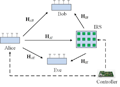
Figure 1: A block diagram of IRS-assisted Gaussian MIMO WTC

III AO Algorithm for Enhancing Secrecy Rate Under Full CSI

In this section, we assume that full CSI is available at Alice, and focus on enhancing the secrecy rate of IRS-assisted MIMO WTC. Based on the aforementioned system setting, the secrecy rate optimization problem of this channel model is expressed as

$${\rm P1}:\underset{{\bf R}\in S_{{\bf R}}{\bf Q}\in S_{{\bf Q}}}{\max}\ C_{s}({\bf R},{\bf Q})=C_{B}-C_{E}$$ (1)

where

$$S_{{\bf R}}\triangleq\{{\bf R}:{\bf R}\geq{\bf 0},{\rm tr}({\bf R})\leq P\},$$

$$S_{{\bf Q}}\triangleq\{{\bf Q}:|q_{i}|=1,\forall i\}$$

denote the feasible set of the transmit covariance ${\bf R}$ and phase shift matrix ${\bf Q}$, respectively, ${\rm tr}({\bf R})\leq P$ is the total power constraint (TPC) at Alice, $P$ denotes total transmit power budget, the unit modulus constraint (UMC) $|q_{i}|=1$ ensures that each reflecting element in IRS does not change the amplitude of the signal. We note that this is a complicated non-convex problem due to non-convex objective function as well as non-convex constraint. Since MIMO setting is considered in this work, all the existing solutions for the MISO case [19]-[26] completely fail to solve ${\rm P1}$ in the full MIMO setting. The reason is that the determinant term in the objective function $C_{B}-C_{E}$ cannot be equivalently simplified to a scalar formular as in the MISO case. Although [27] studied the secrecy rate enhancement of IRS-assisted MIMO WTC, its proposed solution still cannot be directly applied to our considered system model in which the direct link channels ${\bf H}_{AB}$ and ${\bf H}_{AE}$ exist in addition to the reflecting link channels ${\bf H}_{AI}$, ${\bf H}_{IB}$ and ${\bf H}_{IE}$.

Hence, in this section, we develop a numerical solution to solve the non-convex ${\rm P1}$, which is based on AO algorithm to jointly optimize ${\bf R}$ and ${\bf Q}$. The main reason for choosing this algorithm is due to two aspects. Firstly, different from the secrecy capacity of MIMO WTC optimization problem [4]-[7] in which only one variable ${\bf R}$ is considered, there are two variables ${\bf R}$ and ${\bf Q}$ need to be optimized, also note that the objective function $C_{B}-C_{E}$ is a non-convex complicated form and it is difficult to directly obtain the optimal solutions. Hence, the function of AO algorithm is to split the non-convex problem ${\rm P1}$ into two sub-problem with simpler structure by fixing each variable as a constant so that ${\bf R}$, ${\bf Q}$ can be optimized separately in each sub-problem. Secondly, although ${\bf R}$ and ${\bf Q}$ are bounded by the TPC and UMC respectively, these two constraints are independent between each other. Therefore, using AO algorithm, a monotonic convergence of the objective value can be achieved so that a limit point solution of ${\rm P1}$ can be obtained. In our AO algorithm, two new solutions were developed to optimize ${\bf R}$ and ${\bf Q}$ for each sub-problem in the following subsections. When optimizing ${\bf R}$ given fixed ${\bf Q}$, the non-convex sub-problem is firstly equivalently transformed to a convex-concave problem, and a barrier method in combination with Newton method and backtracking line search method is proposed to globally optimize ${\bf R}$. When optimizing ${\bf Q}$ given fixed ${\bf R}$, we propose an OBO optimization method to optimize a sub-optimal solution of ${\bf Q}$.

III-A Barrier Method for Optimizing Transmit Covariance at Alice

In this subsection, we fix phase shift ${\bf Q}$ as a constant and optimize the covariance ${\bf R}$. When ${\bf Q}$ is fixed, the sub-problem of optimizing ${\bf R}$ is expressed as

$${\rm P2}:\underset{{\bf R}\in S_{{\bf R}}}{\max}\ C({\bf R})=\log_{2}\frac{|{\bf I}+{\bf H}_{1}{\bf R}{\bf H}_{1}^{\rm H}|}{|{\bf I}+{\bf H}_{2}{\bf R}{\bf H}_{2}^{\rm H}|}$$ (2)

where ${\bf H}_{1}={\bf H}_{AB}+{\bf H}_{IB}{\bf Q}{\bf H}_{AI},\ \ {\bf H}_{2}={\bf H}_{AE}+{\bf H}_{IE}{\bf Q}{\bf H}_{AI}$. It can be known that this is a standard secrecy capacity optimization problem of Gaussian MIMO WTC. This is a difficult non-convex problem, however, it can be equivalently transformed to a convex-concave formular. By applying the key theorem in [4], ${\rm P2}$ can be equivalently expressed as

$${\rm P3}:\ \max_{{\bf R}\in S_{{\bf R}}}\min_{{\bf K}\in S_{{\bf K}}}f({\bf R},{\bf K})=\log_{2}\frac{|{\bf I}+{\bf K}^{-1}{\bf H}{\bf R}{\bf H}^{\rm H}|}{|{\bf I}+{\bf H}_{2}{\bf R}{\bf H}_{2}^{\rm H}|}$$ (3)

where ${\bf H}=[{\bf H}_{1}^{\rm H},{\bf H}_{2}^{\rm H}]^{\rm H}$, ${\bf K}=E\{\bm{\xi}\bm{\xi}^{\rm H}\}\in\mathbb{C}^{2(d+e)\times 2(d+e)}$, $\bm{\xi}=[\bm{\xi}_{B1}^{\rm H},\bm{\xi}_{B2}^{\rm H},\bm{\xi}_{E1}^{\rm H},\bm{\xi}_{E2}^{\rm H}]^{\rm H}$, $S_{{\bf K}}$ is the feasible set of ${\bf K}$ defined as

$$S_{{\bf K}}\triangleq\left\{{\bf K}:{\bf K}=\begin{bmatrix}{\bf I}&{\bf N}^{\rm H}\\ {\bf N}&{\bf I}\end{bmatrix},\ {\bf K}\geq{\bf 0}\right\}$$ (4)

where ${\bf N}=E\{\bm{\xi}_{E}\bm{\xi}_{B}^{\rm H}\}\in\mathbb{C}^{2e\times 2d}$, $\bm{\xi}_{B}=[\bm{\xi}_{B1}^{\rm H},\bm{\xi}_{B2}^{\rm H}]^{\rm H}$, $\bm{\xi}_{E}=[\bm{\xi}_{E1}^{\rm H},\bm{\xi}_{E2}^{\rm H}]^{\rm H}$. The theorem in [4] indicates that ${\rm P3}$ is a convex-concave optimization problem with saddle point solution, i.e., the objective is concave in ${\bf R}$ for any given ${\bf K}$ and convex in ${\bf K}$ for any given ${\bf R}$ so that Karush-Kuhn-Tucker (KKT) is the sufficient and necessary conditions for optimality. Also the saddle point solution ${\bf R}$ for the max-min problem ${\rm P3}$ is always the optimal solution for the original max problem ${\rm P2}$. Hence, the work left is how to numerically obtain the saddle point solution for ${\rm P3}$. In this subsection, we apply the barrier method illustrated in [5] to solve ${\rm P3}$, which is in combination with Newton method and backtracking line search method. Note that in [5], this method was developed only based on real-valued channel matrix case. In this paper, we improve this algorithm by re-deriving the gradients and Hessians of the barrier function so that it can be used under general complex-valued channel matrix case.

Specifically, by introducing a barrier parameter $t>0$, the constraints can be absorbed by the objective function in P3 so that the barrier function can be expressed as

$$f_{t}({\bf R},{\bf K})= f({\bf R},{\bf K})+t^{-1}\log_{2}(P-tr({\bf R}))$$

$$+t^{-1}\log_{2}|{\bf R}|-t^{-1}\log_{2}|{\bf K}|.$$

Hence, a new optimization problem can be formulated as

$${\rm P4}:\ \max_{{\bf R}\in S^{\prime}_{{\bf R}}}\min_{{\bf K}\in S^{\prime}_{{\bf K}}}\ f_{t}({\bf R},{\bf K})$$ (5)

where $S^{\prime}_{{\bf R}}=\{{\bf R}:{\bf R}>{\bf 0},{\rm tr}({\bf R})<P\},\ S^{\prime}_{{\bf K}}=\{{\bf K}:{\bf K}>{\bf 0}\}$. Since $S^{\prime}_{{\bf R}}\in S_{{\bf R}}$ and $S^{\prime}_{{\bf K}}\in S_{{\bf K}}$, $\rm P4$ is still a convex-concave optimization problem so that KKT conditions is still sufficient and necessary for optimality. Thus, the work reduces to find the saddle point satisfying the KKT conditions $\nabla_{\bf R}f_{t}({\bf R},{\bf K})={\bf 0},\nabla_{\bf K}f_{t}({\bf R},{\bf K})={\bf 0}$. Since the variable ${\bf R}$ and ${\bf K}$ are Hermitian matrices, it is difficult to obtain the gradient (KKT conditions) and Hessians of the objective function. Thus, a vectorization for the variables is needed. Note that in [5], ${\bf R}$ and ${\bf K}$ are symmetric real matrix and its vectorization as well as the obtained gradients and Hessians cannot be directly applied to our complex-valued case. In this paper, we make new vectorization for the complex ${\bf R}$ and ${\bf K}$. Specifically, let ${\bf r}=[{\bf r}_{d}^{\rm T},{\bf r}_{l}^{\rm T},{\bf r}_{l}^{\rm H}]^{\rm T},{\bf n}=[{\rm vec}({\bf N})^{\rm T},{\rm vec}({\bf N})^{\rm H})]^{\rm T}$, where ${\bf r}_{d}$ denotes vectorizing all the diagonal real elements of ${\bf R}$ and ${\bf r}_{l}$ denotes vectorizing all the lower triangular complex elements of ${\bf R}$, then ${\bf r}$ and ${\bf n}$ can be further expressed as the linear transformation ${\bf r}={\bf D}_{{\bf r}}^{\rm T}{\rm vec}({\bf R}),{\bf n}={\bf D}_{{\bf n}}^{\rm T}{\rm vec}({\bf K}-{\bf I})$ where ${\bf D}_{{\bf r}}\in\mathbb{R}^{m^{2}\times m^{2}}$ and ${\bf D}_{{\bf n}}\in\mathbb{R}^{(d+e)^{2}\times 2de}$ are unique full column rank matrices (with the elements either zero and one) satisfying ${\bf D}_{{\bf r}}^{\rm T}{\bf D}_{{\bf r}}={\bf I}$ and ${\bf D}_{{\bf n}}^{\rm T}{\bf D}_{{\bf n}}={\bf I}$. For the details about how to construct ${\bf D}_{{\bf r}}$ and ${\bf D}_{{\bf n}}$, please refer to [31]. Let ${\bf z}=[{\bf r}^{\rm H},{\bf n}^{\rm H}]^{\rm H}$, since ${\bf z}$ can represent all the key information of ${\bf R}$ and ${\bf K}$ completely, the work now further reduces to find the optimal ${\bf z}$ satisfying the new KKT conditions $r({\bf z})=[(\nabla_{{\bf r}^{*}}f_{t}({\bf R},{\bf K}))^{H}\nabla_{{\bf n}^{*}}f_{t}({\bf R},{\bf K})^{H}]^{H}={\bf 0}$. In Newton method, the optimality condition $r({\bf z})={\bf 0}$ is iteratively solved using 1st-order approximation of $r({\bf z})$, which corresponds to the 2nd order approximation of the objective function

$$r({\bf z}_{k}+\Delta{\bf z})=r({\bf z}_{k})+{\bf T}\Delta{\bf z}+o(\Delta{\bf z})={\bf 0}$$ (6)

where ${\bf z}_{k}$ and $\Delta{\bf z}$ are the current variables and their updates at iteration $k$ respectively, and where ${\bf T}$ is the derivative of $r({\bf z})$, i.e., the Hessian matrix of $f_{t}({\bf R},{\bf K})$ in ${\bf r}$ and ${\bf n}$:

$${\bf T}=\begin{bmatrix}\nabla_{{\bf r}^{*}{\bf r}^{\rm T}}^{2}f_{t}({\bf R},{\bf K})&\nabla_{{\bf r}^{*}{\bf n}^{\rm T}}^{2}f_{t}({\bf R},{\bf K})\\ [\nabla_{{\bf r}^{*}{\bf n}^{\rm T}}^{2}f_{t}({\bf R},{\bf K})]^{\rm H}&\nabla_{{\bf n}^{*}{\bf n}^{\rm T}}^{2}f_{t}({\bf R},{\bf K})\end{bmatrix}.$$ (7)

Closed-form expressions for gradients $\nabla_{{\bf r}^{*}}f_{t}({\bf R},{\bf K})$, $\nabla_{{\bf n}^{*}}f_{t}({\bf R},{\bf K})$ and Hessians ${\bf T}$ are given in the Appendix. By ignoring $o(\Delta{\bf z})$, (6) can be further expressed as linear equation

$$r({\bf z}_{k})+{\bf T}\Delta{\bf z}={\bf 0}$$ (8)

so that the update $\Delta{\bf z}$ can be solved numerically from this equation using the existing solver (such as “linsolve” function in Matlab). After that, ${\bf z}$ can be updated as ${\bf z}_{k+1}={\bf z}_{k}+s\Delta{\bf z}$ where $s>0$ denotes the step size which can be found via backtracking line search.

The proposed algorithm for solving P2 is summarized as Algorithm 1. In this algorithm, $\alpha$ is the percentage of the liner decrease for the residual norm $|r({\bf z}_{k})|$ in backtracking line search, $\beta$ controls the reduction in step size at each iteration of backtracking line search, $\eta$ controls the increase of $t$ at each iteration of barrier method, $\epsilon_{1}$ is the required computing accuracy, and $t\in[t_{0},t_{max}]$ where $t_{0}$, $t_{max}$ are the initial and maximum value of $t$ respectively, $({\bf R}_{0},{\bf K}_{0})$ is the feasible starting point satisfying ${\bf R}_{0}\in S^{\prime}_{{\bf R}}$ and ${\bf K}_{0}\in S^{\prime}_{{\bf K}}$. Once the target accuracy of Newton method is reached, the computed $({\bf R}(t),{\bf K}(t))$ is set as the new starting point for the new problem P4 with updated $t$. As $t$ has reached the maximum $t_{max}$, the algorithm stops and output the final solution ${\bf R}$. Note that $t_{max}$ should not be set too high, or the Hessian matrix ${\bf T}$ will get close to singular so that the update $\Delta{\bf z}$ cannot be computed in practice. Using the same steps of proof illustrated in [5], it can be verified that the residual norm $|r({\bf z}_{k})|$ is strictly decreasing in the Newton steps, and also Hessian matrix ${\bf T}$ is non-singular for each $t>0$ so that the solution $\Delta{\bf z}$ is unique during each iteration. Finally, by applying the key properties of barrier method [32], one obtains that as $t\rightarrow\infty$, $f({\bf R}(t),{\bf K}(t))\rightarrow C_{opt}$, from which Algorithm 1 is guaranteed to global convergence.

Algorithm 1 (solving ${\rm P2}$ given fixed ${\bf Q}$)

Require  $({\bf R}_{0},{\bf K}_{0})\rightarrow{\bf z}_{0}$, $0<\alpha<0.5$, $0<\beta<1$, $t_{0}>0$, $t_{max}>t_{0}$, $\mu>1$, $\epsilon_{1}>0$.

1. Set $t=t_{0}$.

repeat  (start barrier method)

     2. Set $k=0$.

     repeat  (start Newton method)

         3. Compute $r({\bf z}_{k})$ for current $k$, and compute update $\Delta{\bf z}$ via (8), and set $s=1$.

         repeat  (start backtracking line search method)

              4. $s:=\beta s$, update ${\bf z}_{k+1}={\bf z}_{k}+s\Delta{\bf z}$.

         until $|r({\bf z}_{k+1})|\leqslant(1-\alpha s)|r({\bf z}_{k})|$ and ${\bf R}_{k+1}\in S^{\prime}_{{\bf R}},{\bf K}_{k+1}\in S^{\prime}_{{\bf K}}$

         5. $k:=k+1$.

     until $|r({\bf z}_{k})|\leqslant\epsilon_{1}$

     6. Set ${\bf z}_{0}:={\bf z}_{k}$ as a new starting point, and update $t:=\mu t$.

until $t>t_{max}$

In Algorithm 1, when $t$ is fixed, the main computational cost comes from the residual norm $r({\bf z}_{k})$, the update $\Delta{\bf z}$ and the loop of backtracking line search in each iteration of Newton method. The complexity of computing $r({\bf z}_{k})$ and $\Delta{\bf z}$ are about $u_{1}=O(m^{4}+(d+e)^{3}+m(d+e)^{2}+em^{2}+2de(d+e)^{2})$ and $u_{2}=O((m^{2}+de)^{3})$ respectively. The complexity of finding the step size $s$ in each iteration of backtracking line search is about $u_{3}=O(m^{2}+de)$. If $l_{b}$ is the total iterations required for backtracking line search to converge, one obtains that the total computation complexity for the current iteration of Newton method is $u_{1}+u_{2}+l_{b}u_{3}$. Furthermore, according to the property of standard barrier method [32], the total number of Newton steps for each value of $t$ scales as $l_{n}=O(log_{2}\epsilon_{1}^{-1}\sqrt{\frac{m(m+1)}{2}+de})$. Thus, the total complexity of Algorithm 1 for each fixed $t$ is $O(l_{n}(u_{1}+u_{2}+l_{b}u_{3}))$.

III-B Algorithm of Optimizing Phase Shift Matrix at the IRS

With the algorithm of optimizing ${\bf R}$ for fixed ${\bf Q}$, the next step is to compute ${\bf Q}$ in this sub-section. The sub-problem of optimizing ${\bf Q}$ given fixed ${\bf R}$ is expressed as ${\rm{P5}}$.

$${\rm{P5}}:\underset{{\bf Q}}{\max}\ C_{s}({\bf R},{\bf Q}),\ s.t.\ |q_{i}|=1,\forall i.$$ (9)

Since the objective function in ${\rm{P5}}$ is a complicated log determinant function, the existing solutions such as semi-definite relaxation and MM in [19][20] fail to solve this problem. Hence, inspired by [18], we propose an OBO optimization method to optimize ${\bf Q}$, in which each one of the $n$ phase shift coefficients are optimized in order by fixing the other $n-1$ coefficients as constant. Note that the system model illustrated in [18] is only an IRS-assisted MIMO channel, and its solution can not be directly applied to our WTC case. Hence, our OBO optimization method is based on the method in [18] but with proper extensions so that a sub-optimal ${\bf Q}$ for ${\rm{P5}}$ can be obtained. Specifically, consider the $i$-th phase shift coefficient is unknown and all the rest $n-1$ coefficients are given, and let the eigenvalue decomposition of ${\bf R}$ is ${\bf R}={\bf U}_{{\bf R}}\bm{\Sigma}_{{\bf R}}{\bf U}_{{\bf R}}^{\rm H}$ where ${\bf U}_{{\bf R}}$ is the unitary matrix, the columns of which are the eigenvectors of ${\bf R}$, $\bm{\Sigma}_{{\bf R}}$ is the diagonal matrix, in which the diagonal entries are eigenvalues of ${\bf R}$. The following proposition concludes the closed-form optimal solutions of $q_{i}$.

Proposition 1.

Given fixed $q_{1},q_{2},...,q_{i-1},q_{i+1},..,q_{n}$, then ${\rm P5}$ can be simplified to the following problem ${\rm P6}$

$${\rm P6}:\underset{q_{i}}{\max}\ C^{\prime}_{B}(q_{i})-C^{\prime}_{E}(q_{i}),\ \ s.t.\ |q_{i}|=1,\forall i$$ (10)

where $C^{\prime}_{B}(q_{i})=\log_{2}|{\bf I}+q_{i}{\bf A}_{i}^{-1}{\bf B}_{i}+q_{i}^{*}{\bf A}_{i}^{-1}{\bf B}_{i}^{\rm H}|$, $C^{\prime}_{E}(q_{i})=\log_{2}|{\bf I}+q_{i}{\bf C}_{i}^{-1}{\bf D}_{i}+q_{i}^{*}{\bf C}_{i}^{-1}{\bf D}_{i}^{\rm H}|$. When ${\rm tr}({\bf A}_{i}^{-1}{\bf B}_{i})={\rm tr}({\bf C}_{i}^{-1}{\bf D}_{i})=0$, then $q_{i}=e^{j\theta_{i}}$ where $\theta_{i}$ can be any value between $0$ and $2\pi$. When ${\rm tr}({\bf A}_{i}^{-1}{\bf B}_{i})\neq 0,{\rm tr}({\bf C}_{i}^{-1}{\bf D}_{i})=0$, then the optimal solution of $q_{i}$ is expressed as $q_{i}=e^{-jarg(\bar{\lambda}_{i})}$, where $\bar{\lambda}_{i}$ is the only non-zero eigenvalue of ${\bf A}_{i}^{-1}{\bf B}_{i}$. When ${\rm tr}({\bf A}_{i}^{-1}{\bf B}_{i})=0,{\rm tr}({\bf C}_{i}^{-1}{\bf D}_{i})\neq 0$, then the optimal solution of $q_{i}$ is expressed as $q_{i}=e^{j(\pi-arg(\tilde{\lambda}_{i}))}$, where $\tilde{\lambda}_{i}$ is the only non-zero eigenvalue of ${\bf C}_{i}^{-1}{\bf D}_{i}$. When ${\rm tr}({\bf A}_{i}^{-1}{\bf B}_{i})\neq 0,{\rm tr}({\bf C}_{i}^{-1}{\bf D}_{i})\neq 0$, then the optimal solution of $q_{i}$ is expressed as $q_{i}=e^{-jarg(\bar{\lambda}_{i}-u\tilde{\lambda}_{i})}$, where $u>0$ is found from BS algorithm.

Proof.

Detailed expressions of ${\bf A}_{i},{\bf B}_{i},{\bf C}_{i},{\bf D}_{i}$ as well as the proof are provided in Appendix. ∎

Based on Proposition 1, the OBO optimization algorithm for optimizing ${\bf Q}$ given ${\bf R}$ is summarized as Algorithm 2. In this algorithm, $q_{i}^{ini}$ is the initialized feasible starting point for each phase shift coefficient. Once all the coefficients are optimized in order, the output ${\bf Q}$ returned by OBO algorithm is a sub-optimal solution of ${\rm P5}$. In this algorithm, the main computational complexity comes from computing the eigenvalue of ${\bf A}_{i}^{-1}{\bf B}_{i}$ and ${\bf C}_{i}^{-1}{\bf D}_{i}$. Hence, if there are $n$ reflecting elements, the total complexity of Algorithm 2 is about $O(2n(d^{3}+e^{3}))$.

Algorithm 2 (OBO optimization algorithm for solving P5 given fixed ${\bf R}$)

Require  $q_{i}^{ini}$, $i=1,2,...n$.

1.Set $i=1$.

repeat  

     2. Compute ${\rm tr}({\bf A}_{i}^{-1}{\bf B}_{i})$ and ${\rm tr}({\bf C}_{i}^{-1}{\bf D}_{i})$.

     3. Obtain the optimal solution of $q_{i}$ according to Proposition 3.

     4. Set $i=i+1$.

until $i=n$

5. Output ${\bf Q}={\rm diag}\{[q_{1},q_{2},...,q_{n}]^{\rm T}\}$ as the sub-optimal solution of P5.

III-C Summary of the AO Algorithm

Finally, with Algorithm 1 and Algorithm 2 at hand, the AO algorithm for maximizing the secrecy rate of IRS-assisted MIMO WTC is summarized as Algorithm 3. Since ${\bf R}$ and ${\bf Q}$ are optimized alternatively, the value of objective function $C_{s}({\bf R},{\bf Q})$ in P1 is non-decreasing with iterations, i.e, $C_{s}({\bf R}_{1},{\bf Q}_{1})\leq C_{s}({\bf R}_{2},{\bf Q}_{2})\leq...\leq C_{s}({\bf R}_{k},{\bf Q}_{k})$, where ${\bf R}_{k}$ and ${\bf Q}_{k}$ is the optimized solution of P2 and P5 returned by Algorithm 1 and Algorithm 2 respectively at iteration $k$. Furthermore, since ${\bf R}$ and ${\bf Q}$ are both bounded by the feasible set $S_{{\bf R}}$ and $S_{{\bf Q}}$ respectively, by applying the Cauchy’s theorem [25], one obtains that a solution ${\bf R}_{opt}$ and ${\bf Q}_{opt}$ always exist such that

$$0 =\underset{k\rightarrow\infty}{\lim}\{C_{s}({\bf R}_{k},{\bf Q}_{k})-C_{s}({\bf R}_{opt},{\bf Q}_{opt})\}$$

$$\leq\underset{k\rightarrow\infty}{\lim}\{C_{s}({\bf R}_{k+1},{\bf Q}_{k+1})-C_{s}({\bf R}_{opt},{\bf Q}_{opt})\}=0,$$

which indicates that Algorithm 3 is guaranteed to converge to a limit point solution of P1.

Algorithm 3 (AO algorithm of solving P1)

Require  $\epsilon_{2}>0$.

1. Set initial point ${\bf R}_{ini}$, ${\bf Q}_{ini}$.

2. Compute $C_{1}=C_{B}-C_{E}$ given ${\bf R}_{ini}$ and ${\bf Q}_{ini}$.

repeat  

     3. Given fixed ${\bf R}_{ini}$, solve the sub-optimal solution ${\bf Q}_{opt}$ of P5 using Algorithm 2.

     4. Solve the global optimal solution ${\bf R}_{opt}$ of P2 given ${\bf Q}_{opt}$ using Algorithm 1.

     5. Compute the current object value $C_{2}=C_{B}-C_{E}$ under ${\bf R}_{opt}$ and ${\bf Q}_{opt}$.

     6. If $|C_{2}-C_{1}|/|C_{1}|>\epsilon_{2}$, set ${\bf Q}_{opt}={\bf Q}_{ini}$ and $C_{1}=C_{2}$, go back to step 3.

until $|C_{2}-C_{1}|/|C_{1}|\leq\epsilon_{2}$

7. Output current ${\bf R}_{opt}$, ${\bf Q}_{opt}$ as the final limit point solution of P1.

IV Enhancing the Secrecy Rate Under no Eve’s CSI

In the previous section, the secrecy rate of IRS-assisted MIMO WTC is optimized based on an ideal assumption that full CSI is available at Alice. In practice, Eve is usually a hidden passive malicious user, it does not actively exchange its CSI with Alice, i.e., the channel matrix ${\bf H}_{AE}$, ${\bf H}_{IE}$ are completely unknown. Therefore, it is unlikely to achieve secure communication by formulating an optimization problem as ${\rm P1}$ under this case. To the best of our knowledge, there is no current research results about how to enhance the secrecy rate in IRS-assisted system without Eve’s CSI.

Inspired by the previous work in [34], in this section, we propose an AN aided joint transmission scheme to enahance the secrecy rate if ${\bf H}_{AE}$, ${\bf H}_{IE}$ are completely unknown at Alice. The main procedure of this scheme is concluded as two steps. In the first step, we minimize a transmit power $P_{min}$ at Alice subject to an achievable rate QoS constraint at Bob. To solve the power minimization problem, a BS and OBO combined AO algorithm is applied to jointly optimizing ${\bf R}$ and ${\bf Q}$. Once the minimum power is obtained, in the second step, AN is applied to jam Eve by using the residual power $P-P_{min}$ at Alice so as to decrease Eve’s channel capacity $C_{E}$. In addition, we also apply this AN aided scheme to a special case where the direct link between Alice and Bob/Eve is blocked (i.e., ${\bf H}_{AB}={\bf 0}$ and ${\bf H}_{AE}={\bf 0}$). In particular, apart from OBO optimization method for optimizing ${\bf Q}$ given ${\bf R}$ for the power minimization problem, we propose an MM algorithm to obtain the sub-optimal ${\bf Q}$ in which all $n$ phase shift coefficients are simultaneously optimized. And we give detailed steps about how to find the proper lower bound (i.e., surrogate function) of the complicated objective function so that MM can be applied to iteratively optimize ${\bf Q}$.

IV-A Power Minimization and AN aided jamming

Firstly, after obtaining the CSI of ${\bf H}_{AI}$ and ${\bf H}_{IB}$ at Alice, a power minimization problem subject to QoS constraint at Bob is formulated as the following ${\rm P9}$.

$${\rm P9}: \underset{{\bf R},{\bf Q}}{\min}\ {\rm tr}({\bf R}),$$

$$s.t.\ \log_{2}|{\bf I}+{\bf H}_{1}{\bf R}{\bf H}_{1}^{\rm H}|\geq\gamma,|q_{i}|=1,\forall i,{\bf R}\geq{\bf 0}$$

where $\log_{2}|{\bf I}+{\bf H}_{1}{\bf R}{\bf H}_{1}^{\rm H}|\geq\gamma$ is the QoS constraint, $\gamma$ is the lowest communication rate requirement at Bob. It can be known that this is also a non-convex problem due to the non-convex QoS constraint and UMC, however, it still can be optimized via AO algorithm. Note that although [13] also addresses to solve a power minimization problem subject to QoS constraints, its solutions only applies for the MISO case and fail to our MIMO case. Therefore, we propose an BS and OBO combined AO algorithm to address the non-convex ${\rm P9}$.

Considering ${\bf Q}$ is fixed, the corresponding sub-problem of optimizing ${\bf R}$ is expressed as ${\rm P10}$.

$${\rm P10}:\underset{{\bf R}}{\min}\ {\rm tr}({\bf R}),\ s.t.\ \log_{2}|{\bf I}+{\bf H}_{1}{\bf R}{\bf H}_{1}^{\rm H}|\geq\gamma,{\bf R}\geq{\bf 0}.$$

To optimize ${\bf R}$ in ${\rm P10}$, we apply the following key proposition.

Proposition 2.

Assume the optimal solution and the corresponding optimal value of P10 is ${\bf R}_{opt}$ and $P_{opt}$ respectively, and consider the following problem

$${\rm P10^{\prime}}: \underset{{\bf R}}{\max}\ C^{\prime}({\bf R})=\log_{2}|{\bf I}+{\bf H}_{1}{\bf R}{\bf H}_{1}^{\rm H}|,$$

$$s.t.\ {\bf R}\geq{\bf 0},{\rm tr}({\bf R})\leq\it{P}_{opt}.$$

Then, the optimal solution and the corresponding optimal value of this problem are also ${\bf R}_{opt}$ and $\gamma$.

Proposition 2 indicates that the optimal solution ${\bf R}_{opt}$ for ${\rm P10}$ also solves the dual problem of maximizing the channel capacity subject to TPC ${\rm tr}({\bf R})\leq P_{opt}$ in ${\rm P10^{\prime}}$. This can be easily shown by contradiction or by comparing the respective KKT conditions of each problem, which are necessary for optimality [5]. Note that the optimal solution ${\bf R}_{opt}$ for ${\rm P10}$ always makes the QoS constraint hold with equality. With this proposition, the work reduces to find a proper $P_{opt}$ such that the optimal value for ${\rm P10^{\prime}}$ is $\gamma$. Since ${\rm P10^{\prime}}$ is a general channel capacity optimization problem, the objective function $C^{\prime}({\bf R})$ is non-decreasing with $P_{opt}$. Hence, BS can be applied to find the proper $P_{opt}$ such that the optimal value $C^{\prime}({\bf R})=\gamma$.

With optimized ${\bf R}$, the next step is to optimize ${\bf Q}$ from the following sub-problem.

$${\rm P11}:{\rm Find}\ {\bf Q},\ s.t.\ \log_{2}|{\bf I}+{\bf H}_{1}{\bf R}{\bf H}_{1}^{\rm H}|\geq\gamma,|q_{i}|=1,\forall i.$$

Note that there is no objective function in this problem, any feasible ${\bf Q}$ satisfying the QoS and UMC can be as the optimal solution for ${\rm P11}$. In fact, if the feasible solution ${\bf Q}$ obtained for ${\rm P11}$ achieves a strictly larger communication rate than the target rate $\gamma$, then the minimum transmit power in ${\rm P10}$ returned by BS can be properly reduced without violating the QoS constraint. Hence, the work reduces to maximize $\log_{2}|{\bf I}+{\bf H}_{1}{\bf R}{\bf H}_{1}^{\rm H}|$ to be as large as possible, which is equivalent to solve the following problem ${\rm P11^{\prime}}$.

$${\rm P11^{\prime}}:\underset{{\bf Q}}{\max}\ \log_{2}|{\bf I}+{\bf H}_{1}{\bf R}{\bf H}_{1}^{\rm H}|,\ s.t.\ |q_{i}|=1,\forall i.$$ (11)

Observing that OBO optimization Algorithm 2 can be easily applied to solve this problem by setting ${\bf H}_{AE}={\bf 0},{\bf H}_{IE}={\bf 0}$ so that given fixed $n-1$ phase shift coefficients, the optimal solution for $q_{i}$ is either $e^{-j{\rm arg}(\bar{\lambda}_{i})}$ or any feasible solution.

The proposed AO algorithm for solving ${\rm P9}$ is summarized as Algorithm 4. In this algorithm, since ${\bf R}$ and ${\bf Q}$ are optimized independently, and also ${\bf R}$ and ${\bf Q}$ are both bounded by the constraints. Hence, the objective function $\rm tr({\bf R})$ is non-increasing in Algorithm 4, and a limit point solution is guaranteed to converge.

Algorithm 4 (AO algorithm of solving P9)

Require  $\epsilon_{3}>0$, $\gamma$.

1. Initialize a feasible starting point ${\bf Q}_{ini}$.

2. Solve P10’ via BS to obtain ${\bf R}_{ini}$ for P9 given ${\bf Q}_{ini}$, compute $P_{0}={\rm tr}({\bf R}_{ini})$.

repeat  

     3. Solve P11’ via OBO optimization to obtain a sub-optimal solution ${\bf Q}_{opt}$ given ${\bf R}_{ini}$.

     4. Solve P10’ via BS to obtain the optimal solution ${\bf R}_{opt}$ for P9 given ${\bf Q}_{opt}$, compute $P_{1}={\rm tr}({\bf R}_{opt})$.

     5. If $|P_{1}-P_{0}|/|P_{0}|>\epsilon_{3}$, set ${\bf R}_{ini}={\bf R}_{opt}$ and $P_{0}=P_{1}$, go back to step 3.

until $|P_{1}-P_{0}|/|P_{0}|\leq\epsilon_{3}$

7. Output ${\bf R}_{opt}$, ${\bf Q}_{opt}$ as the final limit point solution of P9.

After obtaining the minimum power $P_{min}={\rm tr}({\bf R}_{opt})$, the next step is to transmit AN to jam Eve using the residual transmit power $P-P_{min}$. To ensure the QoS at Bob is not affected by AN, we set the directions for signaling AN to $\rm{null}({\bf H}_{1})$, i.e., the null space of the effective channel ${\bf W}_{1}={\bf H}_{1}^{\rm H}{\bf H}_{1}$, and apply equal power allocation to transmit AN to each dimension of ${\rm null}({\bf W}_{1})$. Therefore, the transmit covariance for AN is formulated as

$${\bf R}_{AN}=\frac{P-P_{min}}{m-{\rm rank}({\bf W}_{1})}{\bf U}_{AN}{\bf U}_{AN}^{\rm H}$$ (12)

where the columns in the semi-unitary matrix ${\bf U}_{AN}$ are all $m-{\rm rank}({\bf H}_{1})$ eigenvectors corresponding to zero eigenvalues of ${\bf W}_{1}$. Hence, the final actual achievable secrecy rate by this AN aided joint transmission scheme is

$$C_{s}=\gamma-\log_{2}|{\bf I}+\frac{{\bf H}_{2}{\bf R}{\bf H}_{2}^{\rm H}}{{\bf I}+{\bf H}_{2}{\bf R}_{AN}{\bf H}_{2}^{\rm H}}|.$$ (13)

Note that ${\bf H}_{1}$ should be full row rank matrix so that the null space of ${\bf W}_{1}$ exists. Hence, our proposed scheme only holds for the case when $m>d$. If $m\leq d$, a possible solution is that Bob can turn off some receiving antennas so as to make the number of the rest active antennas to be less than $m$, but the price is that the residual power for AN signaling could be decreased since the degree of freedom between Alice and Bob is reduced so that more transmit power needs to be consumed to meet the QoS constraint.

IV-B A Special Case Where the Direct Link Between Alice-Bob/Eve is Blocked

In this subsection, we consider a special case where the direct communication link between Alice-Bob and Alice-Eve are blocked. Such case has high probability to occur in city’s hot spot, mountainous area, and other indoor environment due to obstacles. Then, the function of IRS is to create a virtual line-of-sight link between Alice and Bob/Eve so as to help the signals bypass the obstacle. And this is the key reason at first why IRS draws great attention by academic and industry. Obviously, the proposed AN aided joint transmission scheme in the previous subsection can be easily applied to this case to enhance the secrecy rate by simply setting ${\bf H}_{AB}={\bf 0}$ and ${\bf H}_{AE}={\bf 0}$. In particular, apart from OBO optimization in the AO algorithm, in this subsection, we propose a MM algorithm to optimize ${\bf Q}$ given ${\bf R}$ for the power minimization problem. The key idea of MM algorithm is to firstly approximate the original non-convex problem to a more tractable formular, in which the objective function is approximated to a linear lower bound (i.e., surrogate function), and then the approximated problem is optimized iteratively by initializing a feasible starting point. If the bound is constructed properly, any converged point generated by MM is a KKT point for the original problem. For detailed explanations of MM, please refer to [35]. Note that different from OBO optimization, all $n$ phase shifts are simultaneously optimized in the MM algorithm.

Specifically, when ${\bf H}_{AB}={\bf 0}$, problem ${\rm P11^{\prime}}$ transfers to the following ${\rm P12}$.

$${\rm P12}: \underset{{\bf Q}}{\max}\ g({\bf Q})=\log_{2}|{\bf I}+{\bf H}_{IB}{\bf Q}{\bf H}_{AI}{\bf R}{\bf H}_{AI}^{\rm H}{\bf Q}^{\rm H}{\bf H}_{IB}^{\rm H}|,$$

$$s.t.\ |q_{i}|=1,\forall i.$$

The following proposition gives the surrogate function of $g({\bf Q})$ as well as the closed-form solutions of ${\bf Q}$ during each iteration of MM algorithm.

Proposition 3.

Let $\tilde{{\bf Q}}$ be a feasible point for ${\rm P12}$, then $g({\bf Q})$ can be lower bounded by

$$g({\bf Q})\geq -2n\lambda_{1}({\bf Z})+2{\rm Re}\{{\bf q}^{\rm H}(\lambda_{1}({\bf Z}){\bf I}-{\bf Z})\tilde{{\bf q}}\}+\tilde{{\bf q}}^{\rm H}{\bf Z}\tilde{{\bf q}}$$

$$+2{\rm Re}\{{\bf q}^{\rm H}{\bf a}_{4}\}+\sum_{j=1}^{2}C_{j}(\tilde{{\bf Q}})=\tilde{g}({\bf Q},\tilde{{\bf Q}})$$

where ${\bf q}=[e^{j\theta_{1}},e^{j\theta_{2}},...,e^{j\theta_{n}}]^{\rm T}$, ${\rm diag}(\tilde{{\bf q}})=\tilde{{\bf Q}}$. Hence the closed-form solution of ${\bf Q}$ given $\tilde{{\bf Q}}$ during each iteration of MM algorithm is given by

$${\bf Q}={\rm diag}([e^{j{\rm arg}(v_{1})},e^{j{\rm arg}(v_{2})},...,e^{j{\rm arg}(v_{n})}]^{\rm T}).$$ (14)

Proof.

To optimize ${\bf Q}$ in ${\rm P12}$ via MM, a proper lower bound of $g({\bf Q})$ should be formulated. Note that $g({\bf Q})$ is a complicated log determinant function, it is difficult to directly obtain its lower bound with only one time approximation as in the MISO case [19][23]. Hence, we apply three successive approximations to obtain the proper lower bound of $g({\bf Q})$ so that MM algorithm can be applied to optimize ${\bf Q}$. Please see detailed expression of ${\bf Z}$, ${\bf q}$, $C_{j}(\tilde{{\bf Q}})$, $v_{i},i=1,2,...,n$ as well as the proof in Appendix. ∎

Therefore, based on this proposition, a KKT solution of ${\rm P12}$ given fixed ${\bf R}$ can be obtained. The BS and MM combined AO algorithm for power minimization when the direct link ${\bf H}_{AB}={\bf 0}$ is summarized as Algorithm 5. In this algorithm, ${\bf Q}_{ini}$ is the starting point for the outer loop of AO algorithm and $\tilde{{\bf Q}}$ is the starting point for the inner loop of MM algorithm. As the convergence is reached, a limit point solution for the power minimization problem can be obtained. In the MM algorithm, the main computational complexity comes from computing $\lambda_{1}({\bf Z})$ in each iteration, which is about $O(2n^{3})$. Once the minimum power satisfying QoS constraint is obtained, AN is used to signalling over the null space of ${\bf H}_{IB}{\bf Q}{\bf H}_{AI}$ using the residual power at Alice so as to jam Eve. Our extensive simulation tests have shown that although Algorithm 5 have less performance on power minimization as well as enhancing secrecy rate compared with Algorithm 4, it has faster speed of convergence with less than around 1 to 5 iterations in most randomly generated channels.

Algorithm 5 (AO algorithm for solving P12)

Require  $\epsilon_{4}>0$, $\gamma$.

1. Initialize a feasible starting point ${\bf Q}_{ini}={\bf I}$, ${\bf R}_{ini}=P{\bf I}/m$, set $P_{0}=P$.

repeat  

     2. Initialize starting point $\tilde{{\bf Q}}={\bf I}$, compute $\tilde{C}_{0}=\tilde{g}(\tilde{{\bf Q}},\tilde{{\bf Q}})$ given ${\bf R}_{ini}$.

     repeat  (MM algorithm)

         3. Optimize ${\bf Q}$ via (14), and compute $\tilde{C}_{1}=\tilde{g}({\bf Q},\tilde{{\bf Q}})$.

         4. If $|\tilde{C}_{1}-\tilde{C}_{0}|/|\tilde{C}_{0}|$ does not converge, set $\tilde{C}_{0}=\tilde{C}_{1}$ and $\tilde{{\bf Q}}={\bf Q}$.

     until $|\tilde{C}_{1}-\tilde{C}_{0}|/|\tilde{C}_{0}|$ converges

     5. Set ${\bf Q}_{opt}={\bf Q}$ as the KKT solution of P12.

     6. Obtain the optimal solution ${\bf R}_{ini}$ via BS given ${\bf Q}_{opt}$, compute $P_{1}={\rm tr}({\bf R}_{opt})$.

     7. If $|P_{1}-P_{0}|/|P_{0}|>\epsilon_{4}$, set ${\bf R}_{ini}={\bf R}_{opt}$ and $P_{0}=P_{1}$, go back to step 3.

until $|P_{1}-P_{0}|/|P_{0}|\leq\epsilon_{4}$

V Simulation Results

To validate the performance of our proposed AO algorithms, extensive simulation results have been carried out in this section. Following [19], we consider a fading environment, and all the channels are formulated as the product of large scale fading and small scale fading. The entries in the small scale fading matrix are randomly generated with complex zero-mean Gaussian random variables with unit covariance. For the large scale fading in all links, the path loss is set as -30dB at reference distance 1m, and path loss exponents for all the links is set as 3. And we assume that the distance between Alice and Bob, Alice and IRS, Alice and Eve, IRS and Bob, IRS and Eve are set as 80m, 30m, 80m, 40m and 40m respectively. In AO Algorithm 3, 4 and 5, we set all the target accuracy as $\epsilon_{2}=\epsilon_{3}=\epsilon_{4}=10^{-4}$, and all the target accuracy for BS algorithm as $10^{-4}$. In addition, $\epsilon_{1}=10^{-8}$, $\alpha=0.3$, $\beta=0.5$, $\eta=5$, $t_{0}=10^{2}$, $t_{max}=10^{5}$ in Algorithm 1 and target accuracy for MM is $10^{-4}$ in Algorithm 5. Note that all the simulation results illustrated in Fig.2 to Fig.4 and Fig.6 are averaged over 100 randomly generated channels, and all the results in Fig.5, Fig.7 to Fig.10 are computed based on single randomly generated channel.

V-A Secrecy Rate of IRS-Assisted MIMO WTC Under Full CSI

In this subsection, the performance of proposed AO Algorithm 3 for maximizing the secrecy rate under full CSI is provided. In Fig.2, we compare the average secrecy rate performance of our AO Algorithm 3 with three benchmark schemes: 1). optimize ${\bf R}$ via Algorithm 1 given zero phase shift (i.e., ${\bf Q}={\bf I}$) at IRS; 2). optimize ${\bf R}$ via Algorithm 1 without IRS (i.e., ${\bf Q}={\bf 0}$); 3). AN aided solutions without IRS in [37]. According to the result, we note that our Algorithm 3 has significantly better performance than the other three benchmark schemes. The main reason is that the reflecting link signals are not only constructively added with the direct link signals at Bob, but also destructively added with the direct link signals at Eve and hence the secrecy rate can be boosted. For the three benchmark schemes, it can be seen that the solution with and without AN under no IRS have very limited performance on enhancing secrecy rate. Furthermore, although zero phase shift solutions with IRS have better performance than that without IRS, it still has a large gap compared with the results returned by Algorithm 3. The reason is that the phase shift ${\bf Q}$ is unchanged, i.e., IRS doesn’t truly change the propagation channels. Therefore, only by jointly optimizing ${\bf R}$ and ${\bf Q}$ can we give full play to the advantages of IRS on enhancing the secrecy performance.

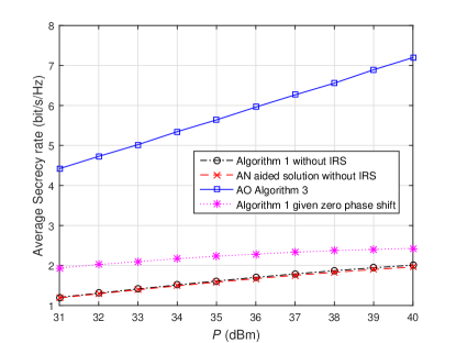
Figure 2: Secrecy rate via proposed AO Algorithm 3 and other benchmark schemes based on $m=d=e=4,n=6$.

Fig.3 illustrate the performance of Algorithm 3 and other benchmark schemes versus the number of reflecting element $n$ at IRS and number of antenna $e$ at Eve respectively. Note that the secrecy rate returned by Algorithm 3 increases with $n$ significantly since more reflecting elements brings more new spacial degree of freedom. Furthermore, for the zero phase shift scheme in which only ${\bf R}$ is optimized, only by increasing $n$ has very limited performance gain on the secrecy rate, even the secrecy rate decreases with $n$. The main reason is that unoptimized ${\bf Q}$ is possible to make the Eve’s effective channel ${\bf H}_{2}$ “better” than Bob’s effective channel ${\bf H}_{1}$. We also note that the secrecy rate returned by Algorithm 3 and other benchmark schemes all decrease with $e$. This is inevitable since with more value of $e$, the sufficient spatial degree of freedom for Alice’s transmission is decreased. However, as can be seen, given fixed $e$, larger secrecy rate still can be obtained by our proposed AO algorithm for the IRS-assisted design than the other solutions. In fact, if Eve is equipped with more antennas, an effective solution is to deploy more reflecting elements at IRS so as to enhance the secrecy rate. This can be easily realized in practical system, since the reflecting elements in IRS are with very low complexity, low power consumption and can be massively deployed.

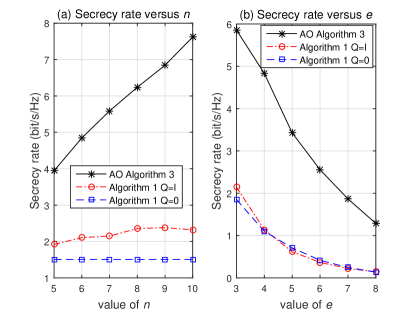
Figure 3: Achieved secrecy rate versus the number of $n$ and $e$, $m=4,d=e=3$ in (a), and $m=d=3,n=6$ in (b).

V-B Secrecy Rate of IRS-Assisted MIMO WTC Under No Eve’s CSI

In this subsection, we provide some simulation results about the performance of proposed AN aided joint transmission scheme on enhancing the secrecy rate under completely no Eve’s CSI. Fig.4 shows the performance of averaged secrecy rate returned by the scheme with and without AN versus the target QoS $\gamma$ at Bob under different settings of $m,n$. Based on the averaged results, note that positive secrecy rate (i.e., $C_{B}>C_{E}$) also can be achieved by our proposed scheme so that secure communication can be guaranteed. Also note that without the aid of AN, only guaranteeing QoS at Bob has very limited performance on enhancing the secrecy rate. In this scheme, as long as $\gamma$ is properly set, Alice could have abundant residual power to jam Eve via AN signalling so that the channel capacity at Alice can be larger than that at Eve. In fact, based on our extensive simulation results, when $\gamma=6$, only about less than $30\%$ of the total transmit power is consumed to meet the QoS constraint by Algorithm 4, and more than half of the total power are all utilized to jam Eve via AN, resulting positive secrecy rate.

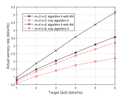
Figure 4: Achieved actual secrecy rate versus Target $\gamma$ under different settings of $m$ and $n$. Total transmit power at Alice is set as $35{\rm dBm}$.

To exploit how the secrecy performance returned by the AN aided scheme goes when the target $\gamma$ is large under no Eve’s CSI, Fig.5 shows the actual secrecy rate versus $\gamma$ under different settings of total power $P$. Note that for each setting of $P$, the secrecy rate firstly increases with $\gamma$, since the transmission rate $C_{B}=\gamma$ at Bob dominates so that $C_{s}$ increases with $\gamma$. However, as $\gamma$ grows to higher, $C_{s}$ starts to decrease, since the sufficient residual power $P-P_{min}$ for AN signaling is reduced significantly so that the information leakage to Eve $C_{E}$ dominates. Finally, as $\gamma$ grows to high enough, the total power $P$ can not support to meet the QoS constraint so that ${\rm P9}$ becomes infeasible and hence secure communication is not achievable (e.g., the secrecy rate stops at $\gamma=10$ when $P=30{\rm dBm}$). Therefore, we see that there is a trade off between increasing QoS at Bob and enhancing the secrecy performance. In addition to this result based on single channel realization, such trade off also exists in our other extensive simulations. Therefore, it is better to balance the setting between $\gamma$ and the residual power $P-P_{min}$ so as to achieve a good secrecy performance.

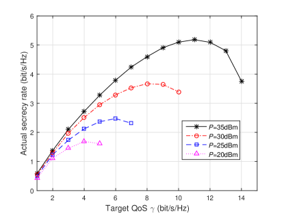
Figure 5: The actual secrecy rate returned by the proposed scheme for no Eve’s CSI versus $\gamma$ given different total power $P$ at Alice . The channels are randomly generated via $m=e=4,d=2,n=8$.

In Fig.6, we assume a special case where the direct link ${\bf H}_{AB}={\bf 0},{\bf H}_{AE}={\bf 0}$, and show the performance of averaged secrecy rate as well as minimized power (to meet the QoS constraint) returned by Algorithm 4 and Algorithm 5 versus $\gamma$. Observing that both Algorithms could guarantee positive secrecy rate, and Algorithm 4 achieves better performance than Algorithm 5, the main reason is that the optimized minimum power returned by Algorithm 4 is less than by Algorithm 5 (see “(b)Minimum transmit power” in Fig.6) and hence more residual power for AN signaling can be saved via Algorithm 4. In addition to this results, our extensive simulation tests based on different channel realizations show that a larger actual secrecy rate can be obtained by Algorithm 4 than that by Algorithm 5 at finite threshold of $\gamma$.

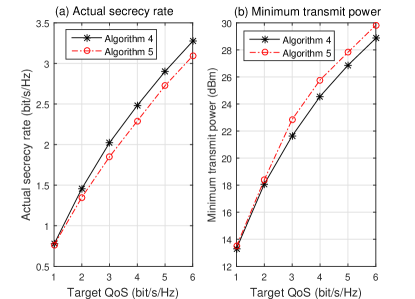
Figure 6: Actual secrecy rate and minimized power versus Target $\gamma$ under ${\bf H}_{AB}={\bf H}_{AE}={\bf 0}$, $m=4,n=8,d=e=2$. Total transmit power at Alice is set as $35{\rm dBm}$.

V-C Convergence of the Proposed AO Algorithms

In this subsection, we provide some numerical examples about the convergence of proposed AO Algorithm 3, 4 and 5 under different value of $m,n,d,e$ and target threshold $\gamma$. Fig.7 illustrates the convergence of the objective function $C_{s}({\bf R}_{k},{\bf Q}_{k})$ versus the number of iterations $k$ in Algorithm 3 under randomly generated channels. Based on the results, it requires 19 to 101 steps for $C_{s}({\bf R}_{k},{\bf Q}_{k})$ to converge to the accuracy of $10^{-4}$ for each considered setting, also note that the process of convergence is monotonically increasing. In fact, given fixed target accuracy, larger settings of $m$ and $n$ leads to larger dimensions of variable ${\bf R}$ and ${\bf Q}$ so that the algorithm requires more iterations to optimize each element of these variables. In addition to these results, our extensive simulations show a perfect monotonic convergence of Algorithm 3.

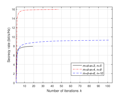
Figure 7: Convergence of the proposed Algorithm 3 under different settings of $m,n,d,e$. $\gamma$ is fixed as 3.

Fig.8 illustrate the convergence of Algorithm 4 for solving ${\rm P9}$. Note that the objective function ${\rm tr}({\bf R}_{k})$ is non-increasing with number of iteration $k$ and finally converge. Furthermore, the convergence is fast with only 5 to 8 steps to reach the target accuracy. Fig.9 compares the convergence between Algorithm 4 and 5 for solving ${\rm P9}$ under ${\bf H}_{AB}={\bf 0}$. As can be seen, Algorithm 5 has a slightly faster convergence with less than 2 to 3 steps compared with Algorithm 4. But when both algorithm converges, the minimum power returned by Algorithm 5 is still less than that by Algorithm 4, which is consistent with those results in Fig.6. In addition to this results, our other extensive simulation tests indicates that a faster speed of convergence (with less than around 1 to 5 steps) than Algorithm 4 can be achieved.

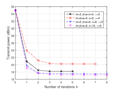
Figure 8: Convergence of the proposed Algorithm 4 under different settings $m,n,d,e$ and $\gamma$. Total transmit power at Alice is set as $35{\rm dBm}$.

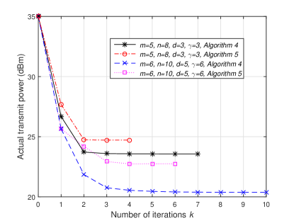
Figure 9: Convergence comparison between Algorithm 4 and 5 when ${\bf H}_{AB}={\bf H}_{AE}={\bf 0}$ under different settings of $m,n,d$ and $\gamma$. Total transmit power at Alice is set as $35{\rm dBm}$.

Finally, Fig.10 shows the convergence of the value of objective function $f({\bf R},{\bf K})$ and $C({\bf R})$ in Algorithm 2 versus number of iterations $k$. It can be noted that both $f({\bf R},{\bf K})$ and $C({\bf R})$ gradually converge and coincide together as $t$ increases to $t_{max}$. In particular, it takes few more steps for $C({\bf R})$ to converge than $f({\bf R},{\bf K})$, which indicates that $C({\bf R})$ is less sensitive in ${\bf R}$ than that in $f({\bf R},{\bf K})$. Hence, it is necessary to set $t_{max}$ large enough in barrier method so that the optimized ${\bf R}$ for P3 is guaranteed to be a global optimal solution for P2. Furthermore, this results also have validated the correctness of our re-derived gradient and Hessians of the barrier objective function $f_{t}({\bf R},{\bf K})$ under complex-valued channel case shown in Appendix.

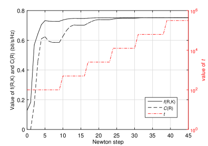
Figure 10: Convergence of $f({\bf R},{\bf K})$ and $C({\bf R})$ in Algorithm 1 when $m=d=e=4,n=6$ and $P=35{\rm dBm}$. As $t$ increases to the threshold $t_{max}$, both $f({\bf R},{\bf K})$ and $C({\bf R})$ converges and coincide together.

VI Concluding Remarks and Future Directions

In this paper, the secrecy rate optimization of IRS-assisted Gaussian MIMO WTC is studied. When full CSI is assumed, a barrier method and OBO optimization combined AO algorithm is proposed to jointly maximize the transmit covariance ${\bf R}$ at Alice as well as phase shift coefficient ${\bf Q}$ at IRS. When no Eve’s CSI is assumed, we propose an AN aided joint transmission scheme to enhance the secrecy rate. In this scheme, a BS and OBO combined AO algorithm is proposed to jointly optimize ${\bf R}$ and ${\bf Q}$. This AN aided scheme is further applied to enhance the secrecy rate under a special scenario where the direct communication between Alice and Bob/Eve is blocked. In particular, a BS and MM combined AO algorithm with slightly faster convergence is proposed to jointly optimize ${\bf R}$ and ${\bf Q}$. Simulation results have validated the monotonic convergence of the proposed algorithms, and it is shown that the proposed algorithms for the IRS-assisted design achieve significantly larger secrecy rate than the other benchmark schemes with and without IRS under full CSI. When Eve’s CSI is unknown, the secrecy performance can also be greatly enhanced by the proposed AN aided joint transmission scheme.

A future direction of our work is to exploit the solutions for enhancing the robust secrecy rate of IRS-assisted MIMO WTC when the CSI of the direct and reflecting channel links are imperfectly known at Alice due to estimation errors. This is a more challenging study since in the secrecy rate optimization problem, the objective function as well as the constraints become more complicated due to the bounded channel estimation errors. Therefore, new numerical algorithm should be redesigned to jointly optimize ${\bf R}$ and ${\bf Q}$ as well as its proof of convergence. The study of robust secure IRS-assisted MIMO channel also provides significant references for the application in practical system design.

VII Appendix

VII-A Closed-form Expressions for Gradients and Hessians in Algorithm 1

After some manipulations, we provide below the analytical expressions for the gradients and Hessians obtained, using the standard rules of matrix differential calculus (see Chapter 3 to 6 in [31]). The gradient of $f_{t}({\bf R},{\bf K})$ respect to ${\bf r}$ and ${\bf n}$ are expressed as

$$\nabla_{{\bf r}^{*}}f_{t}({\bf R},{\bf K})={\bf D}_{{\bf r}}^{\rm T}{\rm vec}(({\bf I}+{\bf H}^{\rm H}{\bf K}^{-1}{\bf H}{\bf R})^{-1}{\bf H}^{\rm H}{\bf K}^{-1}{\bf H}-({\bf I}$$

$$+{\bf H}_{2}^{\rm H}{\bf H}_{2}{\bf R})^{-1}{\bf H}_{2}^{\rm H}{\bf H}_{2}+t^{-1}{\bf R}^{-1}-t^{-1}(P-{\rm tr}({\bf R}))^{-1}{\bf I}),$$

$$\nabla_{{\bf n}^{*}}f_{t}({\bf R},{\bf K})={\bf D}_{{\bf n}}^{\rm T}{\rm vec}(({\bf K}+{\bf H}{\bf R}{\bf H}^{\rm H})^{-1}-(1+t^{-1}){\bf K}^{-1}).$$

Then, each entry of ${\bf T}$ is expressed as

$$\nabla_{{\bf r}^{*}{\bf r}^{\rm T}}^{2}f_{t}({\bf R},{\bf K})=-{\bf D}_{{\bf r}}^{\rm T}({\bf Z}_{1}^{\rm T}\otimes{\bf Z}_{1}-{\bf Z}_{2}^{\rm T}\otimes{\bf Z}_{2}$$

$$+t^{-1}{\bf R}^{-{\rm T}}\otimes{\bf R}^{-1}+t^{-1}(P-{\rm tr}({\bf R}))^{-2}{\rm vec}({\bf I}){\rm vec}({\bf I})^{\rm T}){\bf D}_{{\bf r}},$$

$$\nabla_{{\bf n}^{*}{\bf n}^{\rm T}}^{2}f_{t}({\bf R},{\bf K})=-{\bf D}_{{\bf n}}^{\rm T}({\bf Z}_{3}^{\rm T}\otimes{\bf Z}_{3}$$

$$\quad\quad\quad\quad\quad\quad\quad\quad-(1+t^{-1}){\bf K}^{-{\rm T}}\otimes{\bf K}^{-1}){\bf D}_{{\bf n}},$$

$$\nabla_{{\bf r}^{*}{\bf n}^{\rm T}}^{2}f_{t}({\bf R},{\bf K})=-{\bf D}_{{\bf r}}^{\rm T}({\bf Z}_{4}^{\rm T}\otimes{\bf Z}_{4}^{\rm H}){\bf D}_{{\bf n}}$$

where ${\bf Z}_{1}=({\bf I}+{\bf H}^{\rm H}{\bf K}^{-1}{\bf H}{\bf R})^{-1}{\bf H}^{\rm H}{\bf K}^{-1}{\bf H}$, ${\bf Z}_{2}=({\bf I}+{\bf H}_{2}^{\rm H}{\bf H}_{2}{\bf R})^{-1}{\bf H}_{2}^{\rm H}{\bf H}_{2}$, ${\bf Z}_{3}=({\bf K}+{\bf H}{\bf R}{\bf H}^{\rm H})^{-1}$, ${\bf Z}_{4}={\bf H}^{\rm H}({\bf K}+{\bf H}{\bf R}{\bf H}^{\rm H})^{-1}$.

VII-B Proof of Proposition 1

Firstly, by applying the key steps of deriving (9) and (15) in [18], $C_{B}$ and $C_{E}$ given ${\bf R}$ can be expressed as

$$C_{B}=\log_{2}|{\bf I}+q_{i}{\bf A}_{i}^{-1}{\bf B}_{i}+q_{i}^{*}{\bf A}_{i}^{-1}{\bf B}_{i}^{\rm H}|+\log_{2}|{\bf A}_{i}|,$$

$$C_{E}=\log_{2}|{\bf I}+q_{i}{\bf C}_{i}^{-1}{\bf D}_{i}+q_{i}^{*}{\bf C}_{i}^{-1}{\bf D}_{i}^{\rm H}|+\log_{2}|{\bf C}_{i}|$$

where

$${\bf A}_{i}= {\bf I}+(\bar{{\bf H}}_{AB}+\sum_{j=1,j\neq i}^{n}q_{j}{\bf r}_{j}\bar{{\bf t}}_{j}^{\rm H})(\bar{{\bf H}}_{AB}+\sum_{j=1,j\neq i}^{n}q_{j}{\bf r}_{j}\bar{{\bf t}}_{j}^{\rm H})^{\rm H}$$

$$+{\bf r}_{i}\bar{{\bf t}}_{i}^{\rm H}\bar{{\bf t}}_{i}{\bf r}_{i}^{\rm H},$$

$${\bf B}_{i}= {\bf r}_{i}\bar{{\bf t}}_{i}^{\rm H}(\bar{{\bf H}}_{AB}^{\rm H}+\sum_{j=1,j\neq i}^{n}\bar{{\bf t}}_{j}{\bf r}_{j}^{\rm H}q_{j}^{*}),$$

$${\bf C}_{i}= {\bf I}+(\bar{{\bf H}}_{AE}+\sum_{j=1,j\neq i}^{n}q_{j}{\bf s}_{j}\bar{{\bf t}}_{j}^{\rm H})(\bar{{\bf H}}_{AE}+\sum_{j=1,j\neq i}^{n}q_{j}{\bf s}_{j}\bar{{\bf t}}_{j}^{\rm H})^{\rm H}$$

$$+{\bf s}_{i}\bar{{\bf t}}_{i}^{\rm H}\bar{{\bf t}}_{i}{\bf s}_{i}^{\rm H},$$

$${\bf D}_{i}= {\bf s}_{i}\bar{{\bf t}}_{i}^{\rm H}(\bar{{\bf H}}_{AE}^{\rm H}+\sum_{j=1,j\neq i}^{n}\bar{{\bf t}}_{j}{\bf s}_{j}^{\rm H}q_{j}^{*})$$

and where $\bar{{\bf H}}_{AB}={\bf H}_{AB}{\bf U}_{{\bf R}}\bm{\Sigma}_{{\bf R}}^{0.5}$, $\bar{{\bf H}}_{AE}={\bf H}_{AE}{\bf U}_{{\bf R}}\bm{\Sigma}_{{\bf R}}^{0.5}$, $\bar{{\bf t}}_{i}$ is the $i$-th column of $\bar{{\bf H}}_{AI}^{\rm H}=[{\bf H}_{AI}{\bf U}_{{\bf R}}\bm{\Sigma}_{{\bf R}}^{0.5}]^{\rm H}$, ${\bf r}_{i}$ and ${\bf s}_{i}$ are the $i$-th column of ${\bf H}_{IB}$ and ${\bf H}_{IE}$ respectively. Since ${\bf A}_{i}$ and ${\bf C}_{i}$ are both full rank matrices and ${\rm rank}({\bf B}_{i})\leq 1$, ${\rm rank}({\bf D}_{i})\leq 1$, ${\rm rank}({\bf A}_{i}^{-1}{\bf B}_{i})\leq 1$ and ${\rm rank}({\bf C}_{i}^{-1}{\bf D}_{i})\leq 1$ hold. Hence, by dropping the constant term $\log_{2}|{\bf A}_{i}|$ and $\log_{2}|{\bf C}_{i}|$, ${\rm P5}$ reduces to ${\rm P6}$. It can be known that ${\bf A}_{i}^{-1}{\bf B}_{i}$ and ${\bf C}_{i}^{-1}{\bf D}_{i}$ are strongly related to $q_{i}$. In the following, we consider 4 cases about the trace of ${\bf A}_{i}^{-1}{\bf B}_{i}$ and ${\bf C}_{i}^{-1}{\bf D}_{i}$ and propose the optimal solutions of $q_{i}$ based on each case.

1). Case 1: ${\rm tr}({\bf A}_{i}^{-1}{\bf B}_{i})={\rm tr}({\bf C}_{i}^{-1}{\bf D}_{i})=0$. In this case, both ${\bf A}_{i}^{-1}{\bf B}_{i}$ and ${\bf C}_{i}^{-1}{\bf D}_{i}$ are non diagonalizable according to Lemma 2 in [18]. Therefore, by applying the steps of deriving (21) in [18], the objective function in ${\rm P6}$ is further derived as

$$C^{\prime}_{B}(q_{i})-C^{\prime}_{E}(q_{i})= \log_{2}|{\bf I}-{\bf A}_{i}^{-1}({\bf A}_{i}^{-1}{\bf B}_{i})^{\rm H}{\bf B}_{i}|$$

$$-\log_{2}|{\bf I}-{\bf C}_{i}^{-1}({\bf C}_{i}^{-1}{\bf D}_{i})^{\rm H}{\bf D}_{i}|.$$

Obviously, this objective function is irrelevant to $q_{i}$. Hence, any solution of $q_{i}$ satisfying $|q_{i}|=1$ is the optimal solution of ${\rm P6}$.

2). Case 2: ${\rm tr}({\bf A}_{i}^{-1}{\bf B}_{i})\neq 0,{\rm tr}({\bf C}_{i}^{-1}{\bf D}_{i})=0$. In this case, ${\bf A}_{i}^{-1}{\bf B}_{i}$ is diagonalizable and $C^{\prime}_{E}(q_{i})$ is not affected by $q_{i}$. Let the eigenvalue decomposition of ${\bf A}_{i}^{-1}{\bf B}_{i}$ as ${\bf A}_{i}^{-1}{\bf B}_{i}=\bar{{\bf U}}_{i}\bar{\bm{\Sigma}}_{i}\bar{{\bf U}}_{i}^{\rm H}$, where $\bar{{\bf U}}_{i}$ is the unitary matrix, the columns of which are the eigenvectors, $\bar{\bm{\Sigma}}_{i}={\rm diag}\{\bar{\lambda}_{i},0,...0\}$, and let $\bar{{\bf V}}_{i}=\bar{{\bf U}}_{i}^{\rm H}{\bf A}_{i}\bar{{\bf U}}_{i}$, $\bar{{\bf v}}_{i}$ denotes the first column of $\bar{{\bf V}}_{i}^{-1}$, $\bar{{\bf v}}_{i}^{{}^{\prime}{\rm T}}$ denotes the first row of $\bar{{\bf V}}_{i}$. By applying the key steps of deriving (16) and (17) in [18], $C^{\prime}_{B}(q_{i})$ is further expressed as

$$C^{\prime}_{B}(q_{i})=\log_{2}(1+\bar{\lambda}_{i}^{2}(1-\bar{v}_{i1}^{{}^{\prime}}\bar{v}_{i1})+2{\rm Re}\{q_{i}\bar{\lambda}_{i}\})$$ (15)

where $\bar{v}_{i1}$ and $\bar{v}_{i1}^{{}^{\prime}}$ are the first elements in $\bar{{\bf v}}_{i}$ and $\bar{{\bf v}}_{i}^{{}^{\prime}{\rm T}}$ respectively. Therefore, it can be directly obtained that the optimal solution for maximizing $C^{\prime}_{B}(q_{i})$ is $q_{i}=e^{-jarg(\bar{\lambda}_{i})}$.

3). Case 3: ${\rm tr}({\bf A}_{i}^{-1}{\bf B}_{i})=0,{\rm tr}({\bf C}_{i}^{-1}{\bf D}_{i})\neq 0$. In this case, ${\bf C}_{i}^{-1}{\bf D}_{i}$ is diagonalizable and $C^{\prime}_{B}(q_{i})$ is not affected by $q_{i}$. Let the eigenvalue decomposition of ${\bf C}_{i}^{-1}{\bf D}_{i}$ as ${\bf C}_{i}^{-1}{\bf D}_{i}=\tilde{{\bf U}}_{i}\tilde{\bm{\Sigma}}_{i}\tilde{{\bf U}}_{i}^{\rm H}$, where $\tilde{{\bf U}}_{i}$ is the unitary matrix, the columns of which are the eigenvectors, $\tilde{\bm{\Sigma}}_{i}={\rm diag}\{\tilde{\lambda}_{i},0,...0\}$, and let $\tilde{{\bf V}}_{i}=\tilde{{\bf U}}_{i}^{\rm H}{\bf C}_{i}\tilde{{\bf U}}_{i}$, $\tilde{{\bf v}}_{i}$ denotes the first column of $\tilde{{\bf V}}_{i}^{-1}$, $\tilde{{\bf v}}_{i}^{{}^{\prime}{\rm T}}$ denotes the first row of $\tilde{{\bf V}}_{i}$. Similar with (15), $C^{\prime}_{E}(q_{i})$ can be further expressed as

$$C^{\prime}_{E}(q_{i})=\log_{2}(1+\tilde{\lambda}_{i}^{2}(1-\tilde{v}_{i1}^{{}^{\prime}}\tilde{v}_{i1})+2{\rm Re}\{q_{i}\tilde{\lambda}_{i}\})$$ (16)

where $\tilde{v}_{i1}$ and $\tilde{v}_{i1}^{{}^{\prime}}$ are the first elements in $\tilde{{\bf v}}_{i}$ and $\tilde{{\bf v}}_{i}^{{}^{\prime}{\rm T}}$ respectively. Hence, to maximize P6, the work reduces to minimize $C^{\prime}_{E}(q_{i})$, i.e., ${\rm Re}\{q_{i}\bar{\lambda}_{i}\}$ should be minimized. Therefore, it can be directly obtained that the optimal solution for minimizing $C^{\prime}_{E}(q_{i})$ is $q_{i}=e^{j(\pi-arg(\tilde{\lambda}_{i}))}$.

4). Case 4: ${\rm tr}({\bf A}_{i}^{-1}{\bf B}_{i})\neq 0,{\rm tr}({\bf C}_{i}^{-1}{\bf D}_{i})\neq 0$. In this case, both ${\bf A}_{i}^{-1}{\bf B}_{i}$ and ${\bf C}_{i}^{-1}{\bf D}_{i}$ are diagonalizable so that the both $C^{\prime}_{B}(q_{i})$ and $C^{\prime}_{E}(q_{i})$ are related to $q_{i}$. By combining (15) and (16) together, ${\rm P6}$ can be further expressed as

$${\rm P7}:\underset{q_{i}}{\max}\ \frac{\bar{c}_{i}+2{\rm Re}\{q_{i}\bar{\lambda}_{i}\}}{\tilde{c}_{i}+2{\rm Re}\{q_{i}\tilde{\lambda}_{i}\}},\ s.t.\ |q_{i}|=1,\forall i$$ (17)

where $\bar{c}=1+\bar{\lambda}_{i}^{2}(1-\bar{v}_{i1}^{{}^{\prime}}\bar{v}_{i1}),\tilde{c}=1+\tilde{\lambda}_{i}^{2}(1-\tilde{v}_{i1}^{{}^{\prime}}\tilde{v}_{i1})$. P7 is a fractional programming optimization problem, which can be solved via Dinkelback method. Let $u\geq 0$, and then we consider the following problem.

$${\rm P8}: \underset{q_{i}}{\max}\ f(q_{i}/u)=\bar{c}_{i}+2{\rm Re}\{q_{i}\bar{\lambda}_{i}\}-u(\tilde{c}_{i}+2{\rm Re}\{q_{i}\tilde{\lambda}_{i}\}),$$

$$s.t.\ |q_{i}|=1,\forall i.$$

Hence, according to the key concept of Dinkelbach method, finding the optimal solution of ${\rm P7}$ is equivalently to finding the proper value of $u$ such that the optimal value of the objective function $f(q_{i}/u)$ in P8 is zero. To obtain the proper $u$, the following key lemma is needed.

Lemma 1.

Consider $q_{i}^{opt}$ is the optimal solution given fixed $u$ in P8, then $f(q_{i}^{opt}/u)$ is a monotonically decreasing function in $u$.

Proof.

Assume $0<u_{1}<u_{2}$, and denote $q_{i}^{opt1}$ and $q_{i}^{opt2}$ to be the optimal solution of P8 given $u_{1}$ and $u_{2}$ respectively, then

$$f(q_{i}^{opt2}/u_{2}) =\bar{c}_{i}+2{\rm Re}\{q_{i}^{opt2}\bar{\lambda}_{i}\}-u_{2}(\tilde{c}_{i}+2{\rm Re}\{q_{i}^{opt2}\tilde{\lambda}_{i}\})$$

$$<\bar{c}_{i}+2{\rm Re}\{q_{i}^{opt2}\bar{\lambda}_{i}\}-u_{1}(\tilde{c}_{i}+2{\rm Re}\{q_{i}^{opt2}\tilde{\lambda}_{i}\})$$

$$\leq\bar{c}_{i}+2{\rm Re}\{q_{i}^{opt1}\bar{\lambda}_{i}\}-u_{1}(\tilde{c}_{i}+2{\rm Re}\{q_{i}^{opt1}\tilde{\lambda}_{i}\})$$

$$=f(q_{i}^{opt1}/u_{1}).$$ (18)

Hence, $f(q_{i}^{opt2}/u_{2})<f(q_{i}^{opt1}/u_{1})$, from which the proof is complete. ∎

Based on this key lemma, BS algorithm can be applied to find the optimal $u$ such that $f(q_{i}^{opt}/u)=0$. Note that $f(q_{i}/u)$ can be further expressed as $f(q_{i}/u)=\bar{c}_{i}-u\tilde{c}_{i}+2{\rm Re}\{q_{i}(\bar{\lambda}_{i}-u\tilde{\lambda}_{i})\}$. Hence, once the optimal $u$ is obtained, it can be directly obtained that the optimal solution for minimizing $C^{\prime}_{E}(q_{i})$ is $q_{i}=e^{-jarg(\bar{\lambda}_{i}-u\tilde{\lambda}_{i})}$, from which the proof is complete.

VII-C Proof of Proposition 3

Firstly, let ${\bf P}={\bf H}_{IB}{\bf Q}{\bf L}^{\frac{1}{2}}$, ${\bf L}={\bf H}_{AI}{\bf R}{\bf H}_{AI}^{\rm H}$, according to matrix inversion lemma, $g({\bf Q})$ can be further expressed as $g({\bf Q})=-\log_{2}|{\bf I}-{\bf P}({\bf I}+{\bf P}^{\rm H}{\bf P})^{-1}{\bf P}^{\rm H}|$. To find the lower bound of $g({\bf Q})$, we firstly introduce the following key lemma.

Lemma 2.

For any matrix ${\bf A}\in\mathbb{C}^{m\times m}$ and $\tilde{{\bf A}}\in\mathbb{C}^{m\times m}$,

$$\log_{2}|{\bf A}|\leq\log_{2}|\tilde{{\bf A}}|+{\rm tr}(\tilde{{\bf A}}^{-1}({\bf A}-\tilde{{\bf A}})).$$ (19)

(19) holds since $\log_{2}|{\bf A}|$ is concave in ${\bf A}$. Hence, let ${\bf Q}_{B}={\bf I}-{\bf P}({\bf I}+{\bf P}^{\rm H}{\bf P})^{-1}{\bf P}^{\rm H}$ and consider $\tilde{{\bf Q}}$ is a feasible point satisfying the unit modulus constraint, then $g({\bf Q})$ can be lower bounded by

$$g({\bf Q}) \geq-\log_{2}|\tilde{{\bf Q}}_{B}|-{\rm tr}(\tilde{{\bf Q}}_{B}^{-1}({\bf Q}_{B}-\tilde{{\bf Q}}_{B}))$$

$$=C_{1}(\tilde{{\bf Q}})+h_{B}({\bf Q})$$

where $C_{1}(\tilde{{\bf Q}})=-\log_{2}|\tilde{{\bf Q}}_{B}|+{\rm tr}({\bf I})-{\rm tr}(\tilde{{\bf Q}}_{B}^{-1})$, $h_{B}({\bf Q})={\rm tr}(\tilde{{\bf Q}}_{B}^{-1}{\bf P}({\bf I}+{\bf P}^{\rm H}{\bf P})^{-1}{\bf P}^{\rm H})$, $\tilde{{\bf Q}}_{B}={\bf I}-\tilde{{\bf P}}({\bf I}+\tilde{{\bf P}}^{\rm H}\tilde{{\bf P}})^{-1}\tilde{{\bf P}}^{\rm H}$, $\tilde{{\bf P}}={\bf H}_{IB}\tilde{{\bf Q}}{\bf L}^{\frac{1}{2}}$. It can be verified that $C_{1}(\tilde{{\bf Q}})+h_{B}({\bf Q})$ is a surrogate function of $g({\bf Q})$ so that P12 is approximated to the following ${\rm P13}$.

$${\rm P13}:\underset{{\bf Q}}{\max}\ C_{1}(\tilde{{\bf Q}})+h_{B}({\bf Q}),\ s.t.,|q_{i}|=1.$$ (20)

However, it is still difficult to apply MM algorithm to solve this problem due to the complicate structure of $h_{B}({\bf Q})$ as well as non-convex UMC. Hence, we apply a second approximation of $g({\bf Q})$ by finding a lower bound of $h_{B}({\bf Q})$. The following key lemma of matrix fractional functions is need to construct this bound [32].

Lemma 3.

For any positive semi-definite matrix ${\bf A}\in\mathbb{C}^{m\times m}$ and positive definite matrix ${\bf B},\tilde{{\bf B}}\in\mathbb{C}^{n\times n}$, and ${\bf X},\tilde{{\bf X}}\in\mathbb{C}^{m\times n}$,

$${\rm tr}({\bf A}{\bf X}{\bf B}^{-1}{\bf X}^{\rm H})$$

$$\geq {\rm tr}({\bf A}\tilde{{\bf X}}\tilde{{\bf B}}^{-1}\tilde{{\bf X}}^{\rm H})-{\rm tr}({\bf A}\tilde{{\bf X}}\tilde{{\bf B}}^{-1}({\bf B}-\tilde{{\bf B}})\tilde{{\bf B}}^{-1}\tilde{{\bf X}}^{\rm H})$$

$$+{\rm tr}({\bf A}({\bf X}-\tilde{{\bf X}})\tilde{{\bf B}}^{-1}\tilde{{\bf X}}^{\rm H})+{\rm tr}({\bf A}\tilde{{\bf X}}\tilde{{\bf B}}^{-1}({\bf X}-\tilde{{\bf X}})^{\rm H}).$$

Lemma 3 holds since ${\rm tr}({\bf A}{\bf X}{\bf B}^{-1}{\bf X}^{\rm H})$ is equivalent to the sum of m matrix fractional functions, and thus convex [32]. Therefore, by applying this lemma to the term $h_{B}({\bf Q})$ via setting ${\bf A}=\tilde{{\bf Q}}_{B}^{-1}$, ${\bf X}={\bf P}$, $\tilde{{\bf X}}=\tilde{{\bf P}}={\bf H}_{IB}\tilde{{\bf Q}}{\bf L}^{\frac{1}{2}}$, ${\bf B}={\bf I}+{\bf P}^{\rm H}{\bf P}$ and $\tilde{{\bf B}}={\bf I}+\tilde{{\bf P}}^{\rm H}\tilde{{\bf P}}$ and after some manipulations, the lower bound of $g({\bf Q})$ can be further expressed as

$$g({\bf Q})\geq C_{1}(\tilde{{\bf Q}})+h_{B}({\bf Q})\geq\sum_{i=1}^{2}C_{i}(\tilde{{\bf Q}})+g_{B}({\bf Q})$$ (21)

where $C_{2}(\tilde{{\bf Q}})=-{\rm tr}(\tilde{{\bf Q}}_{B}^{-1})+{\rm tr}(\tilde{{\bf Q}}_{B}^{-1}{\bf J}_{B}\tilde{{\bf P}}^{\rm H}\tilde{{\bf P}}{\bf J}_{B}^{\rm H})$, $g_{B}({\bf Q})=-{\rm tr}(\tilde{{\bf Q}}_{B}^{-1}{\bf J}_{B}{\bf P}^{\rm H}{\bf P}{\bf J}_{B}^{\rm H})+{\rm tr}(\tilde{{\bf Q}}_{B}^{-1}{\bf J}_{B}{\bf P}^{\rm H})+{\rm tr}({\bf P}{\bf J}_{B}^{\rm H}\tilde{{\bf Q}}_{B}^{-1})$ and where ${\bf J}_{B}=\tilde{{\bf P}}({\bf I}+\tilde{{\bf P}}^{\rm H}\tilde{{\bf P}})^{-1}$. In the following, we express $g_{B}({\bf Q})$ to a more tractable form. Let ${\bf A}_{1}=\tilde{{\bf Q}}_{B}^{-1}{\bf J}_{B}{\bf L}^{\frac{1}{2}},{\bf A}_{2}={\bf H}_{IB}^{\rm H}{\bf H}_{IB},{\bf A}_{3}={\bf L}^{\frac{1}{2}}{\bf J}_{B}^{\rm H},{\bf A}_{4}={\bf H}_{IB}^{\rm H}\tilde{{\bf Q}}_{B}^{-1}{\bf J}_{B}{\bf L}^{\frac{1}{2}}$, by applying the lemma of matrix identity in [36] that for any matrix ${\bf A}$, ${\bf B}$ and diagonal matrix ${\bf V}$ with proper sizes, ${\rm tr}({\bf V}^{\rm H}{\bf A}{\bf V}{\bf B})={\bf v}^{\rm H}({\bf A}\odot{\bf B}^{\rm T}){\bf v}$ holds where the entries in ${\bf v}$ are all diagonal elements in ${\bf V}$, $g_{B}({\bf Q})$ can be further expressed as

$$g_{B}({\bf Q}) =-{\rm tr}({\bf Q}^{\rm H}{\bf A}_{2}{\bf Q}{\bf A}_{3}{\bf A}_{1})+{\rm tr}({\bf A}_{4}{\bf Q}^{\rm H})+{\rm tr}({\bf Q}{\bf A}_{4}^{\rm H})$$

$$=-g_{b}({\bf q})+2{\rm Re}\{{\bf q}^{\rm H}{\bf a}_{4}\}$$ (22)

where $g_{b}({\bf q})={\bf q}^{\rm H}{\bf Z}{\bf q}$, ${\bf Z}={\bf A}_{2}\odot({\bf A}_{3}{\bf A}_{1})^{\rm T}$ and where the entries in ${\bf a}_{4}$ are all diagonal entires in ${\bf A}_{4}$. Hence, P13 can be further approximated to ${\rm P14}$.

$${\rm P14}: \underset{{\bf q}}{\max}\ -g_{b}({\bf q})+2{\rm Re}\{{\bf q}^{\rm H}{\bf a}_{4}\}+\sum_{j=1}^{2}C_{j}(\tilde{{\bf Q}}),$$

$$s.t.\ |q_{i}|=1,\forall i.$$

We note that the objective function in P14 is quadratic concave in ${\bf q}$, however, it is still difficult to solve this problem due to non-convex UMC. Hence, we apply the following lemma, from which the proof can be found in [35].

Lemma 4.

Let ${\bf X}$ be an $n\times n$ Hermitian matrix, then for any point $\tilde{{\bf a}}\in\mathbb{C}^{n\times 1}$, ${\bf a}^{\rm H}{\bf X}{\bf a}$ is upper bounded by ${\bf a}^{\rm H}{\bf X}{\bf a}\leq{\bf a}^{\rm H}{\bf Y}{\bf a}-2Re\{{\bf a}^{\rm H}({\bf Y}-{\bf X})\tilde{{\bf a}}\}+\tilde{{\bf a}}^{\rm H}({\bf Y}-{\bf X})\tilde{{\bf a}}$, where ${\bf Y}=\lambda_{1}({\bf X}){\bf I}$.

Using this lemma, given a feasible point $\tilde{{\bf q}}$, a surrogate function of $g_{b}({\bf q})$ can be expressed as

$$g_{b}({\bf q}) \leq{\bf q}^{\rm H}\lambda_{1}({\bf Z}){\bf I}{\bf q}-2{\rm Re}\{{\bf q}^{\rm H}(\lambda_{1}({\bf Z}){\bf I}-{\bf Z})\tilde{{\bf q}}\}$$

$$\quad+\tilde{{\bf q}}^{\rm H}(\lambda_{1}({\bf Z}){\bf I}-{\bf Z})\tilde{{\bf q}}$$

$$=2n\lambda_{1}({\bf Z})-2{\rm Re}\{{\bf q}^{\rm H}(\lambda_{1}({\bf Z}){\bf I}-{\bf Z})\tilde{{\bf q}}\}-\tilde{{\bf q}}^{\rm H}{\bf Z}\tilde{{\bf q}}$$ (23)

where $\tilde{{\bf q}}$ is the feasible point, the entries of which are the diagonal entries of $\tilde{{\bf Q}}$. Hence, combing (21), (22) and (23), $g({\bf Q})\geq\tilde{g}({\bf Q},\tilde{{\bf Q}})$ follows. It can be also verified that $\tilde{g}({\bf Q},\tilde{{\bf Q}})$ is a surrogate function of $g({\bf Q})$. By dropping the constant term in $\tilde{g}({\bf Q},\tilde{{\bf Q}})$, ${\rm P14}$ is finally approximated to $\max_{{\bf q}}{\rm Re}\{{\bf q}^{\rm H}{\bf v}\},s.t.\ |{\bf q}_{i}|=1$, where ${\bf v}=(\lambda_{1}({\bf Z}){\bf I}-{\bf Z})\tilde{{\bf q}}+{\bf a}_{4}$. Obviously, the objective function ${\rm Re}\{{\bf q}^{\rm H}{\bf v}\}$ is maximized only when the phase of ${\bf q}$ and ${\bf v}$ are equal. Thus, the closed-form global optimal solution for P15 is expressed as (14) where $v_{i}$ denotes the $i$-th elements of ${\bf v}$, from which the proof is complete.

References

• [1] M. Bloch and J. Barros, β€œPhysical-layer security: from information theory to security engineering,” Cambridge University Press, 2011.
• [2] A. Khisti and G.W. Wornell, β€œSecure transmission with multiple antennas – part I: The MISOME wiretap channel,” IEEE Trans. Inf. Theory, vol. 56, no. 7, Jul. 2010.
• [3] Q. Li and W. K. Ma, β€œSpatially selective artificial-noise aided transmit optimization for MISO Multi-Eves secrecy rate maximization,” IEEE Trans. Signal Process., vol. 61, no. 10, pp. 2704–2717, May 2013.
• [4] A. Khisti and G.W. Wornell, β€œSecure transmission with multiple antennasβ€”part II: The MIMOME wiretap channel,” IEEE Trans. Inf. Theory, vol. 56, no. 11, pp. 5515-5532, Nov. 2010.
• [5] S. Loyka and C. D. Charalambous, β€œAn algorithm for global maximization of secrecy rates in Gaussian MIMO wiretap channels,” IEEE Trans. Commun., vol. 63, no. 6, pp. 2288-2299, June. 2015.
• [6] L. Dong, S. Loyka, and Y. Li, β€œThe secrecy capacity of Gaussian MIMO wiretap channels under interference constraints,” IEEE J. Sel. Areas Commun., vol. 36, no. 4, pp. 704-722, Apr. 2018.
• [7] S.Loyka and L. Dong, β€œOptimal full-rank signaling over MIMO wiretap channels under interference constraint,” IEEE Wireless Commun. Letters, vol. 7, no. 4, pp. 534-537, Aug. 2018.
• [8] Y. Wu et al., β€œA survey of physical layer security techniques for 5G wireless networks and challenges ,” IEEE J. Sel. Areas Commun., vol. 36, no. 4, pp. 679-695, Apr. 2018.
• [9] J. Zhao, β€œA survey of intelligent reflecting surfaces (IRSs): Towards 6G wireless communication networks with massive MIMO 2.0,” 2019, arXiv:1907.04789. [Online]. Available: https://arxiv.org/pdf/1907.04789
• [10] S. Hu, F. Rusek, and O. Edfor, β€œBeyond massive MIMO: The potential of data transmission with large intelligent surfaces,” IEEE Trans Signal Process., vol. 66, no. 10, pp. 2746-2758, Mar. 2018.
• [11] K. Ntontin, et al., β€œReconfigurable intelligent surfaces vs. relaying: Differences, similarities, and performance comparison,” IEEE Open J. Commun. Soc., vol. 1, pp. 798-807, Jul. 2020.
• [12] Q. Wu and R. Zhang, β€œTowards smart and reconfigurable environment: Intelligent reflecting surface aided wireless network,” IEEE Commun. Magazine, vol. 58, no. 1, pp. 106-112, Jan. 2020.
• [13] Q. Wu and R. Zhang, β€œIntelligent reflecting surface enhanced wireless network via Joint active and passive beamforming,” IEEE Trans. Wireless Commun.,vol. 18, no. 11, pp. 5394-5409, Nov. 2019.
• [14] Q. Wu and R. Zhang, β€œBeamforming optimization for intelligent reflecting surface with discrete phase shifts.” 2019 IEEE International Conference on Acoustics, Speech and Signal Processing (ICASSP), Brighton, UK, 2019.
• [15] C. Huang, A. Zappone, M. Debbah, and C. Yuen, β€œAchievable rate maximization by passive intelligent mirrors,” IEEE International Conference on Acoustics, Speech and Signal Processing (ICASSP), Calgary, Canada, Apr. 2018.
• [16] C. Huang, A. Zappone, G. C. Alexandropoulos, M. Debbah, and C. Yuen, β€œReconfigurable intelligent surfaces for energy efficiency in wireless communication,” IEEE Trans. Wireless Commun., vol. 18, no. 8, pp. 4157-4170, Aug. 2019.
• [17] C. Huang, G C. Alexandropoulos, A. Zappone, M. Debbah, and C. Yuen, β€œEnergy efficient multi-user MISO communication using low resolution large intelligent surfaces,” IEEE Globecom Workshops (GC WKshps), Abu Dhabi, United Arab Emirates, 2018.
• [18] S. Zhang and R. Zhang, β€œCapacity characterization for intelligent reflecting surface aided MIMO communication,” IEEE J. Sel. Commun., to be published, DOI: 10.1109/JSAC.2020.3000814.
• [19] H. Shen, W. Xu, S. Gong, Z. He, and C. Zhao, β€œSecrecy rate maximization for intelligent reflecting surface assisted multi-antenna communications,” IEEE Commun. Letters, vol. 23, no. 9, pp. 1488-1492, Sep. 2019.
• [20] M. Cui, G. Zhang, and R. Zhang, β€œSecure wireless communication via intelligent reflecting surface,” IEEE Wireless Commun. Letters, vol. 8, no. 5, pp. 1410-1414, Oct. 2019.
• [21] Y. Song, M. R. A. Khandaker, F. Tariq, and K.-K. Wong, β€œTruly intelligent reflecting surface-aided secure communication using deep learning,” 2019, arXiv:2004.03056. [Online]. Available: https://arxiv.org/abs/2004.03056.
• [22] C. Zheng, W. Hao, P. Xiao, and J. Shi, β€œIntelligent reflecting surface aided multi-antenna secure transmission,” IEEE Wireless Commun. Letters, vol. 9, no. 1, pp. 108-112, Jan. 2020.
• [23] X. Yu and R. Schober, β€œEnabling secure wireless communications via intelligent reflecting surfaces,” in Proc. IEEE Global Commun. Conf. (GLOBECOM), Waikoloa, HI, USA, Dec. 2019, pp. 1-6.
• [24] B. Feng, Y. Wu, and M. Zheng, β€œSecure transmission strategy for intelligent reflecting surface enhanced wireless system,” 2019 11th International Conference on Wireless Communications and Signal Processing (WCSP), Xi’an, China, 2019.
• [25] J. Chen ,Y. Liang , Y. Pei, and H. Guo, β€œIntelligent reflecting surface: A programmable wireless environment for physical layer security,” IEEE Access, vol. 7, pp. 82599-82612, Jun. 2019.
• [26] D. Xu et al., β€œResource allocation for secure IRS-assisted multiuser MISO systems,” 2019 IEEE Globecom Workshops (GC WKshps), Waikoloa, HI, USA, Dec. 2019.
• [27] L. Dong, H.-M. Wang, β€œSecure MIMO transmission via intelligent reflecting surface,” IEEE Wireless Commun. Letters, vol. 9, no. 6, pp. 787-790, Jun. 2020.
• [28] Z. Wang, L. Liu, and S. Cui, β€œ Channel estimation for intelligent reflecting surface assisted multiuser communications,” 2020 IEEE Wireless Communications and Networking Conference (WCNC), Seoul, Korea (South), May 2020.
• [29] Z.-Q. He and X. Yuan, β€œCascaded channel estimation for large intelligent metasurface assisted massive MIMO,” IEEE Wireless Commun. Letters, vol. 9, no. 2, pp. 210-214, Feb. 2020.
• [30] J. Mirza and B. Ali, β€œChannel Estimation Method and Phase Shift Design for Reconfigurable Intelligent Surface Assisted MIMO Networks,” 2019, arXiv:1912.10671. [Online]. Available: https://arxiv.org/abs/1912.10671
• [31] A. Hjorungnes, β€œComplex-valued matrix derivatives: With applications in signal processing and communications,” Cambridge University Press, 2011.
• [32] S. Boyd and L. Vandenberghe, β€œConvex Optimization,” Cambridge University Press, 2004.
• [33] F. Zhang, β€œMatrix theory: Basic results and techniques,” Springer, 1999.
• [34] H.-M. Wang, Q. Yin, and X. Xia, β€œDistributed beamforming for physical-layer security of two-way relay networks,” IEEE Trans. Signal Process., vol. 60, no. 7, pp. 3532-3545, Jul. 2012.
• [35] Y. Sun, P. Babu, and D. P. Palomar, β€œMajorization-minimization algorithms in signal processing, communications, and machine learning,” IEEE Trans. Signal Process., vol. 65, no. 3, pp. 794-816, Feb. 2017.
• [36] X.-D. Zhang, β€œMatrix analysis and applications,” Cambridge University Press, 2017.
• [37] B. Fang, Z. Qian, W. Zhong, and W. Shao, β€œAN-aided secrecy precoding for SWIPT in cognitive MIMO broadcast channels,” IEEE Commun. Letters, vol. 19, no. 9, pp. 1632-1635, Sep. 2015.