Johnson Cook Flow Stress Parameter for Free Cutting Steel 50SiB8

Abstract

The present publication deals with the material characterization of the free cutting steel 50SiB8 for numerical simulations. Quasi-static tensile tests as well as Split Hopkinson Tension Bar (SHTB) tests at various strain rates and temperatures are used to deduce the parameters for a Johnson-Cook flow stress model. These parameters are then verified against the SHTB-experiments within a finite element model (FEM) of the SHTB-test within ABAQUS^©.

1 Introduction

The relatively new material 50SiB8 [4, 11] was developed by Swiss Steel^© as a lead free alternative for classical free cutting steels, e.g. 11SMnPb30 and 16MnCrS5Pb. The development became necessary as regulatory requirements have tightened and in future may ban vehicle components containing heavy metals, such as lead [5]. The idea is to exchange lead by graphite inclusions in order to keep the good machinability of free cuttings steels. As the data basis for numerical simulations of this material is rather small [13, 1, 7], this report is initiated in support to [7], where the results of quasi-static tensile tests and Split Hopkinson Tension Bar (SHTB) tests were used to derive a modified Johnson-Cook fracture strain model for the free cutting steel 50SiB8. Here, the same test results are used to deduce the parameters for a flow stress model according to Johnson and Cook [8]. The model is commonly used to describe metal plasticity within machining simulations and is given as:

$$\sigma_{y}=\underbrace{\left(A+B\cdot\varepsilon_{pl}^{n}\right)}_{\text{1st term}}\hskip 8.53581pt\underbrace{\left[1+C\cdot ln\frac{\dot{\varepsilon}_{pl}}{\dot{\varepsilon}^{0}_{pl}}\right]}_{\text{2nd term}}\hskip 8.53581pt\underbrace{\left[1-\left(\frac{T-T_{ref}}{T_{f}-T_{ref}}\right)^{m}\right]}_{\text{3rd term}}$$ (1)

with $A$, $B$, $C$, $m$ and $n$ being material parameters, $\varepsilon_{pl}$ the plastic strain, $\dot{\varepsilon}_{pl}$ the plastic strain rate and $T$ the current temperature. $T_{f}$ is the melting temperature, $T_{ref}$ is the reference temperature and $\dot{\varepsilon}_{pl}^{0}$ the reference plastic strain rate. The first two terms describe hardening due to plastic strain and plastic strain rate, respectively. The third term controls thermal softening upon increasing temperature. The approach used here for the derivation of its 5 material parameters mainly follows [9, 2].

2 Experimental Procedure

Quasi-static and dynamic tests were performed. The complete test matrix is given with table 1 while test details are provided in the subsequent sections 2.1 and 2.2.

Temperature	$20^{\circ}C$	$200^{\circ}C$	$400^{\circ}C$	$600^{\circ}C$	$800^{\circ}C$	Test specimen	Test
Strain Rate
$0.001s^{-1}$	3	-	-	-	-	ø=6mm, figure 1	quasi-static (tensile)
$500s^{-1}$	4	3	3	3	3	ø=3mm, figure 3	dynamic (SHTB)
$900s^{-1}$	4	3	3	3	3	ø=3mm, figure 3	dynamic (SHTB)
$1700s^{-1}$	4	-	-	-	-	ø=3mm, figure 3	dynamic (SHTB)

Table 1: Static and dynamic test matrix with number of tests

2.1 Quasi-Static Tensile Tests

Three tensile tests were performed at room temperature (293.15K ) at a very low strain rate of $\dot{\varepsilon}=0,001/s$, see also table 1. The low strain rate ensures almost quasi-static conditions. Unnotched test specimen were used with a diameter of 6mm. A drawing of the test specimen is shown in figure 1.

Figure 1: Drawing of the quasi-static tensile test specimen according to [13]

The engineering stress-strain curves were recorded and are shown in figure 2. From these measurements the Johnson-Cook parameters A, B and n were fitted, see section 3.2.

Figure 2: Engineering stress-strain curves from quasi-static tests at room temperature

2.2 Testing at Higher Strain Rates

Tests at higher strain rates were performed by means of the SHTB device with unnotched specimen and a diameter of 3mm. A drawing [13] of the SHTB test specimen is provided with figure 3. After the tests for every SHTB test the average strain rate was evaluated between initial yield point and ultimate tensile strength [6].

Figure 3: Drawing of the SHTB test specimen according to [13]

More details about the test setup are provided in [13, 7]. The results were used to identify:

• the strain rate dependency (parameter C) at room temperature 293.15K for targeted strain rates of 500/s, 900/s and $\approx 1700/s$, each test with 4 repetitions and

• the temperature dependency (parameter m) at room temperature and at elevated temperatures of $200^{\circ}C$, $400^{\circ}C$, $600^{\circ}C$ and $800^{\circ}C$ and targeted strain rates of 500/s and 900/s.

All conducted SHTB tests are compiled in table 1.

3 Material Parameter Determination

3.1 Assessment of True Stress and True Strain

During the measurements engineering strain and stress values were recorded and were later converted into true strains and stresses. Until uniform elongation $A_{G}$ the conversion can be performed by the following equations given in [2]:

$$\varepsilon_{true}=ln(1+\varepsilon_{eng})$$ (2)

and

$$\sigma_{true}=\sigma_{eng}\cdot(1+\varepsilon_{eng})$$ (3)

The true strain in equation (2) consists of elastic and plastic contributions. According to [2], assuming an additive split of both components, the true plastic strain can be computed by:

$$\varepsilon_{true}^{pl}=\varepsilon_{true}-\varepsilon^{el}_{true}=\varepsilon_{true}-\frac{\sigma_{true}}{E}$$ (4)

Beyond uniform elongation $A_{G}$ the conversions (2) and (3) are invalid. The determination of true stresses and strains would require ad-hoc tracking of the progressively reducing diameter in the necking zone which is not performed in this investigation. Instead, the true strain at fracture $\varepsilon_{f}$ can be computed from the measurement of initial $D_{i}$ and fracture diameter $D_{f}$ of the specimen according to [2]:

$$\varepsilon_{f}=ln\left(\frac{A_{i}}{A_{f}}\right)=ln\left(\frac{D_{i}^{2}}{D_{f}^{2}}\right)$$ (5)

The corresponding true stress $\sigma_{f}$ at fracture is then computed from the force at fracture $F_{f}$ and the fracture surface area $A_{f}$:

$$\sigma_{f}=\frac{F_{f}}{A_{f}}$$ (6)

3.2 Parameter A, B and n from Quasi-Static Tests at Room Temperature

Quasi-static tensile test results at room temperature were used to derive the parameters A, B and n for the static part (first term) of the Johnson-Cook flow stress model (1):

$$\sigma_{y}^{static}=A+B\cdot\varepsilon_{pl}^{n}$$ (7)

The measured stresses and strains until uniform elongation $A_{G}$ were converted into true plastic strains and true stresses by use of equations (2), (3) and (4). Additionally, the stresses and strains at fracture were incorporated to the true stress- true plastic strain data. They were computed by equations (5) and (6) based on measured initial $D_{i}$ and fracture diameter $D_{f}$ of the specimen and the force at fracture $F_{f}$, see table 2.

Specimen	$D_{i}$	$D_{f}$	Force at fracture $F_{f}$	$\varepsilon_{f}$	$\sigma_{f}$
1	$6.00mm$	$4.75mm$	$18716N$	$46.72\%$	$1056MPa$
2	$5.99mm$	$4.66mm$	$18298N$	$50.22\%$	$1073MPa$
3	$5.99mm$	$4.62mm$	$18637N$	$51.94\%$	$1112MPa$

Table 2: Fracture stresses and strains from quasi-static tests

The latter approach follows the proposal of [2] and shall improve predictions of the flow stress curve at higher strains towards fracture.

A least squares fit is used to fit the parameters A, B and n from equation (7) to the experimental data, by minimizing the sum of the squared error of the model prediction [3]:

$$\sum_{i}\left[\sigma_{y}^{static}(\varepsilon_{pl}^{n})-\sigma_{y,i}^{measured}(\varepsilon_{pl})\right]^{2}=\sum_{i}\left[A+B\cdot\varepsilon_{pl}^{n}-\sigma_{y,i}^{measured}(\varepsilon_{pl})\right]^{2}=min$$ (8)

The permissible bounds for the three parameters within the least squares fit are given in table 3.

	A [MPa]	B [MPa]	n [-]
Minimum	$430.9(R_{eL})$	0	0
Maximum	$434.5(R_{eH})$	6000	5.999

Table 3: Limits for the static yield stress coefficients A, B and n within the least squares fit

The coefficient $A$ was limited between lower ($R_{eL}$) and upper ($R_{eH}$) yield stress from quasi-static tensile tests at room temperature and thus reflecting the initial yield stress of a virgin material.

A [MPa]	B [MPa]	n [-]	$R^{2}$-value	Comments
430.9	908.7	0.3854	0.8262	with fracture data
430.9	1605.7	0.5829	-	without fracture data

Table 4: Least squares fit of Johnson-Cook coefficients A, B & n

The resulting parameters of the least squares fit are compiled in table 4. The first parameter set considers the fracture stress-strains, while the second set does not. Figure 4 shows the measured stress-strain curves at quasi-static conditions as well as the fitted flow stress curves. The red curve (second set in table 4) represents the fit without consideration of fracture data while the blue curve considers. It can be seen that without including fracture data into the parameter fit the flow stress is predicted to be higher at larger plastic strains and the fracture energy is significantly increased, which is expressed in the difference of the surface areas under the red and blue curve. Since the blue curve gives a better overall fit of the static yield limit part of the JC flow stress equation (7), its parameters (first set in table 4) are used in the subsequent work.

Figure 4: Quasi-static tensile test results and curve fit with (blue) and without (red) consideration of fracture stress-strains

The quality of the least squares fit is determined by the $R^{2}$-value[10] which is determined by:

$$R^{2}=1-\frac{\sum\limits_{i}(y_{i}-\hat{y}_{i})^{2}}{\sum\limits_{i}(y_{i}-\bar{y})^{2}}$$ (9)

with $y_{i}$ the measured value, $\hat{y}_{i}$ the predicted value and $\bar{y}$ the mean value of the measured values. Inserting the flow stresses from the measurement $\sigma_{y,i}^{measured}(\varepsilon_{pl})$, the flow stresses from the prediction $\sigma_{y,i}^{static}(\varepsilon_{pl})$ and the measured mean value $\bar{\sigma}_{y,i}^{measured}(\varepsilon_{pl})$:

$$R^{2}=1-\frac{\sum\limits_{i}(\sigma_{y,i}^{measured}(\varepsilon_{pl})-\sigma_{y,i}^{static}(\varepsilon_{pl}))^{2}}{\sum\limits_{i}(\sigma_{y,i}^{measured}(\varepsilon_{pl})-\bar{\sigma}_{y,i}^{measured}(\varepsilon_{pl}))^{2}}$$ (10)

gives $R^{2}=0.8262$ for the parameter set including fracture data. This is not a perfect fit but is considered to be acceptable.

3.3 Data Preparation for Determination of Parameters C and m

Before evaluation of parameters $C$ and $m$ all true stresses and true strains converted from equations (2) and (3) were smoothed because of overlayed oscillations in the measurement data, see for example figure 26. Each experimental flow stress curve was first smoothed by fitting it to a polynomial, inspired by [2, 9]. The polynomial chosen here is of the same type as the first term of the Johnson-Cook flow stress equation (1):

$$\sigma_{i}^{smoothed}(\varepsilon_{pl})=a_{i}+b_{i}\cdot\varepsilon_{pl}^{c_{i}}$$ (11)

where $i$ is the experiment number. The fit of the polynomial coeffcients $a_{i},b_{i}$ and $c_{i}$ was performed in the range from initial yielding point until uniform strain $A_{G,i}$ using a least squares algorithm as in section 3.2. The permissible bounds for the coefficients $a_{i},b_{i}$ and $c_{i}$ where:

-	$a_{i}$ [MPa]	$b_{i}$ [MPa]	$c_{i}$ [-]
Minimum	$0$	$0$	0
Maximum	$1200$	$5000$	5.999

Table 5: Least square fit limits for coefficients $a_{i}$, $b_{i}$ and $c_{i}$

From these polynomials flow stresses $\sigma_{i}^{smoothed}$ were then evaluated at a plastic strain of $\varepsilon_{pl}=5\%$:

$$\sigma_{i}^{smoothed}(\varepsilon_{pl}=5\%)=a_{i}+b_{i}\cdot(0.05)^{c_{i}}$$ (12)

These flow stresses are required in the following sections for the determination of the parameters C and m of the Johnson-Cook flow stress model. The coefficients $a_{i},b_{i}$ and $c_{i}$, the $R^{2}$-value of the fit as well as the flow stress at $\varepsilon_{pl}=5\%$ are provided with table 6.

Test	Temperature	Average	Uniform	$a_{i}$	$b_{i}$	$c_{i}$	$R^{2}$-value	Flow Stress
i	$T_{i}[^{\circ}C]$	Strain Rate	strain	[MPa]	[MPa]	[-]	$\varepsilon^{pl}\leq A_{G,i}$	$\sigma_{i}^{smoothed}$ at
		$\dot{\varepsilon}^{i}_{pl}[s^{-1}]$	$A_{G,i}[\%]$					$\varepsilon_{pl}=5\%$ [MPa]
1	$20$	0.001	13.8	232.1	1326.1	0.332	0.9855	723
2	$20$	0.001	13.6	244.2	1321	0.338	0.9854	723.8
3	$20$	0.001	13.7	249.2	1323.9	0.339	0.9851	729.2
4	$20$	472.72	13.1	548.1	1313.6	0.631	0.9818	746.4
5	$20$	479.09	14.3	563.7	1440.7	0.718	0.9719	731.3
6	$20$	484.03	15	548.1	1134.5	0.616	0.9671	727.2
7	$20$	491.11	13.4	549.6	1220.6	0.639	0.9836	729.6
8	$20$	887.49	13.3	616.5	1676.7	0.779	0.9155	779.2
9	$20$	894.47	14.5	606.1	1347	0.687	0.9478	778.1
10	$20$	899.75	14.1	602.8	1417.1	0.728	0.9453	762.8
11	$20$	907.23	13.3	588.6	1483.6	0.741	0.9446	749.7
12	$20$	1617.94	13.9	696.5	2493.4	1.064	0.8076	799.5
13	$20$	1642.95	14	637.8	1913.6	0.937	0.8551	753.4
14	$20$	1678.04	14.7	700.5	2381.8	1.096	0.6981	789.7
15	$20$	1757.72	9.6	731.8	2591.3	1.331	0.7851	779.8
16	$200$	454.28	14	408.6	969.6	0.52	0.9563	612.7
17	$200$	463.12	14.6	418.6	998.6	0.512	0.9752	633.8
18	$200$	464.06	13.4	415.9	1015	0.538	0.9646	618.5
19	$200$	876.9	12.3	507.7	1391.5	0.731	0.8981	663.2
20	$200$	885.76	13.8	488.5	1179	0.68	0.8899	642.3
21	$200$	898.29	13.4	483.7	1180.6	0.695	0.9136	630.7
22	$400$	504.61	13.1	359.4	956.5	0.607	0.884	514.4
23	$400$	509.95	12.7	337.5	860.5	0.544	0.9525	506.3
24	$400$	510.56	12	333.9	865.8	0.529	0.9571	511.4
25	$400$	938.53	12.2	422.6	1764.1	0.981	0.7484	515.8
26	$400$	954.49	12.9	401.2	1082	0.747	0.8645	516.5
27	$400$	954.8	13.8	381.7	914.1	0.635	0.8992	518.3
28	$600$	446.04	11.3	311.8	1188.8	0.522	0.9672	561
29	$600$	468.76	12	293.7	1067.8	0.503	0.9748	530.5
30	$600$	476.82	13.9	297.6	1116.6	0.574	0.9595	497.9
31	$600$	747.06	11.7	548.4	1474.7	0.617	0.9858	780.9
32	$600$	919.24	14.2	349	1044.4	0.59	0.9635	527.6
33	$600$	924.23	14.4	330	1043.2	0.595	0.9672	505.3
34	$800$	444.75	20.4	235.3	533.6	0.601	0.9922	323.3
35	$800$	448.05	22.6	238.8	552.7	0.614	0.9811	326.6
36	$800$	471.62	24.3	191.4	591.3	0.625	0.9785	282.4
37	$800$	893.21	22	260.4	692	0.739	0.9724	336
38	$800$	897.57	22	248.4	687.8	0.726	0.976	326.5
39	$800$	921.92	25.9	184.8	670.8	0.675	0.9829	273.6

Table 6: Overview of all conducted tests. For every test the curve fit parameters $a_{i},b_{i}$ and $c_{i}$, and the corresponding flow stress $\sigma_{i}^{smoothed}$ at $\varepsilon_{pl}=5\%$ is given.

3.3.1 Parameter C

The parameter C of the JC flow stress was fitted from flow stress measurements taken at room temperature (293.15K ) and four different strain rates, corresponding to the data sets 1-15 in table 6. The flow stresses were evaluated at a plastic strain of $\varepsilon_{pl}=5\%$. Each flowstress $\sigma_{i}^{smoothed}(\varepsilon_{pl}=5\%)$ was divided by the static yield stress $\sigma_{y}^{static}=\sigma_{y}(\varepsilon_{pl}=0.0,\dot{\varepsilon}_{pl}=0.001s^{-1},T=293.15K)$ giving the yield stress ratio $r^{dyn}_{\sigma,i}$ between static and dynamic yield stress for each test:

$$r^{dyn}_{\sigma,i}=\frac{\sigma_{i}^{smoothed}(\varepsilon_{pl}=5\%)}{\sigma_{y}^{static}(\varepsilon_{pl}=5\%)}=\left[1+C\cdot ln\frac{\dot{\varepsilon}_{pl,i}}{\dot{\varepsilon}^{0}_{pl}}\right]$$ (13)

The reference strain rate was set to the strain rate of the quasi-static tests with $\dot{\varepsilon}^{0}_{pl}=10^{-3}s^{-1}$. Finally, all yield stress ratios $r^{dyn}_{\sigma,i}$ were then used to find the parameter C by a least squares fit:

$$\sum_{i}\left(r^{dyn}_{\sigma,i}-\left[1+C\cdot ln\frac{\dot{\varepsilon}_{pl,i}}{\dot{\varepsilon}^{0}_{pl}}\right]\right)^{2}=min$$ (14)

In figure 5 the synthetic flow stresses from table 6 at different strain rates are shown for a plastic strain of $\varepsilon_{pl}=5\%$ at room temperature (T=293.15K ). The same results, but with a logarithmic scale of the the strain rate is shown in figure 6.

Figure 5: Flow stresses at $\varepsilon_{pl}=0.05$ and various strain rates at room temperature: measured values (blue crosses), predicted at experimental strain rates (red crosses) and continuous curve (orange dotted) in the range from $\dot{\varepsilon}_{pl}=0/s..2000/s$.

Figure 6: Strain rate sensitivity of the yield stress, logarithmic scale

The fitted parameter C is given in table 7 including the $R^{2}$-value according to equation (9).

C [-]	$\mathbf{\dot{\varepsilon}^{0}_{pl}}[s^{-1}]$	$\mathbf{R^{2}}[-]$
0.00447	$10^{-3}$	0.35

Table 7: Least squares fit of Johnson-Cook coefficient C

The $R^{2}$-value is rather low, indicating a poor fit to the experimental data as already visible in figure 5. A similar strain rate dependency is visible also in the investigation of Thimm [14] on a C45E steel (1.1191). A straight line would give a better fit here, at least in the tested strain rate range from $0/s$ to $1700/s$, but would result in questionable predictions at higher strain rates and is therefore not followed up. It has to be noted that even with a low $R^{2}$-value here the overall error in the yield stress is comparably small as the strain rate sensitivity of this material is with $C=0.00447$ rather low.

3.3.2 Parameter m

The parameter $m$ was determined similar to the strain rate sensitivity $C$ but here utilizing yield stresses $\sigma_{i}^{smoothed}(\varepsilon_{pl}=5\%)$ for all temperatures and strain rates, see data sets 1-39 in table 6. Then, the yield stress ratios $r_{\sigma,i}^{temp}$ to the first two terms of the Johnson-Cook flow stress model:

$$r_{\sigma,i}^{temp}=\frac{\sigma_{i}^{smoothed}(\varepsilon_{pl}=5\%)}{\left(A+B\cdot\varepsilon_{pl}^{n}\right)\hskip 8.53581pt\left[1+C\cdot ln\frac{\dot{\varepsilon}_{pl}}{\dot{\varepsilon}^{0}_{pl}}\right]}=\left[1-\left(\frac{T_{i}-T_{ref}}{T_{f}-T_{ref}}\right)^{m}\right]$$ (15)

as well as the corresponding homologous temperatures:

$$T_{i}^{*}=\frac{T_{i}-T_{ref}}{T_{f}-T_{ref}}$$ (16)

were determined, where the melting temperature is $T_{f}=2006K$ [13] and the reference temperature $T_{ref}=293.15K$ corresponds to the static tests at room temperature. Figure 7 shows the yield stress ratios versus homologous temperature. While the general trend is a decreasing yield stress with increasing temperature, a peak exists with large scatter around $T^{*}=0.35$ ($T=600^{\circ}C$). First, the parameter m was fitted based on all data points by least squares:

$$\sum_{i}\left(r_{\sigma,i}^{temp}-\left[1-\left(T_{i}^{*}\right)^{m}\right]\right)^{2}=min$$ (17)

giving the coefficient m. The fitted curve is shown in red in figure 7. For the temperatures $T=20^{\circ}C$ and $T=200^{\circ}C$ the fit lies in the scatter band of the measured data, while it predicts higher yield stresses at $T=400^{\circ}C$ and $T=800^{\circ}C$. At $T=600^{\circ}C$ the yield stress is predicted too low as the scatter of the experimental data is very large and ranges from $\approx 65\%$ to $100\%$ of the yield stress at $T=20^{\circ}C$. This issue is probably due to blue brittleness as discussed in [7]. The classic Johnson-Cook temperature term is not able to correctly describe this behaviour and the curve fit is worsened before and after this peak. Therefore, another curve fit (green curve) was performed, not using experimental data from $T=600^{\circ}C$ at all. Thus, predictions for $T=400^{\circ}C$ and $T=800^{\circ}C$ are improved, while at $T=600^{\circ}C$ worsened a bit. This is considered as an acceptable compromise, since the peak at $T=600^{\circ}C$ cannot be captured anyway.

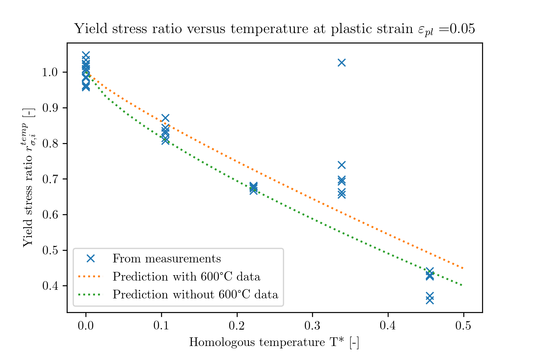
Figure 7: Yield stress ratio versus homologous temperature $T^{*}$

The two fitted parameters m are given in table 8 including the $R^{2}$-values according to equation (9). Beside the outlier in the range of $T^{*}=0.35$ ($T=600^{\circ}C$), the second fit can predict with acceptable accuracy the temperature characteristics and is therefore used in the following.

m [-]	$R^{2}$	$R^{2}$	Comment
	$T=20..800^{\circ}C$	without $T=600^{\circ}C$
0.8584	0.83	0.95	fit to all data, red curve in figure 7
0.7361	0.80	0.98	without data at $T=600^{\circ}C$, green curve in figure 7

Table 8: Least squares fit of Johnson-Cook coefficient m

3.4 Complete Parameter Set

All coefficients for the Johnson-Cook flow stress model are compiled in table 9.

A [MPa]	B [MPa]	C [-]	m [-]	n [-]	$\dot{\varepsilon}^{pl}_{0}[s^{-1}]$	$T_{ref}$
430.9	908.7	0.00447	0.7361	0.3854	$10^{-3}$	293.15K

Table 9: Final Johnson-Cook flow stress model coefficients

4 Comparison of Measured and Predicted Flow Stresses

In this section the parameter set from table 9 for the Johnson-Cook flow stress model is used to compare analytical flow stress predictions versus selected stress-strain curves from the measurements. All analyzed cases are given in table 10.

Strain Rate $[s^{-1}]$	$T=20^{\circ}C$	$T=200^{\circ}C$	$T=400^{\circ}C$	$T=600^{\circ}C$	$T=800^{\circ}C$
0.001	$\surd$	-	-	-	-
500	$\surd$	-	-	-	-
900	$\surd$	$\surd$	$\surd$	$\surd$	$\surd$
1700	$\surd$	-	-	-	-

Table 10: Simulated strain rates and temperatures

In this comparison the dissipation of plastic work into heat (adiabatic heating) is not considered. The graphical results are shown in figure 8 to figure 15. In general the JC model constants from table 9 adequately fit to the measurements, with an exception at a temperature of $T=600^{\circ}C$ which was already to expect. This issue was already discussed in section 3.3.2. Another observation is the high oscillations in the experimental data mainly at the beginning of the measurement as well as larger scatter especially at temperatures of $T=600^{\circ}C$ and $T=800^{\circ}C$

Figure 8: Predicted and experimental flow stress curve at $T=20^{\circ}C,\dot{\varepsilon}_{pl}=0.001s^{-1}$

Figure 9: Predicted and experimental flow stress curve at $T=20^{\circ}C,\dot{\varepsilon}_{pl}=500s^{-1}$

Figure 10: Predicted and experimental flow stress curve at $T=20^{\circ}C,\dot{\varepsilon}_{pl}=900s^{-1}$

Figure 11: Predicted and experimental flow stress curve at $T=20^{\circ}C,\dot{\varepsilon}_{pl}=1700s^{-1}$

Figure 12: Predicted and experimental flow stress curve at $T=200^{\circ}C,\dot{\varepsilon}_{pl}=900s^{-1}$

Figure 13: Predicted and experimental flow stress curve at $T=400^{\circ}C,\dot{\varepsilon}_{pl}=900s^{-1}$

Figure 14: Predicted and experimental flow stress curve at $T=600^{\circ}C,\dot{\varepsilon}_{pl}=900s^{-1}$

Figure 15: Predicted and experimental flow stress curve at $T=800^{\circ}C,\dot{\varepsilon}_{pl}=900s^{-1}$

5 Numerical Validation

The fitted parameter set for the Johnson-Cook flow stress model was used to numerically simulate the quasi-static tensile test and the SHTB tests. The results (engineering stresses and strains) are then compared to the experimentally obtained values. The simulations were carried out with Abaqus 6-14.1 and the explicit solver.

5.1 Geometry and Mesh

The geometries were built in Abaqus/CAE according to specimen drawings from figure 2 and figure 3 and are shown in figure 16 and 18. The geometries were meshed with elements of the type C3D8R. The quasi-static tensile test specimen consists of 7084 elements with 8370 nodes, a picture is provided with figure 17. The SHTB-test specimen consists of 14032 elements with 16154 nodes, a picture is provided with figure 19.

Figure 16: Geometry of the quasi-static tensile test specimen

Figure 17: FE-mesh of the quasi-static tensile test specimen

Figure 18: Geometry of the SHTB test specimen

Figure 19: FE-mesh of the SHTB test specimen

5.1.1 Material Parameters

The test specimen material is 50SiB8. As described in the introduction a flow stress model according to Johnson and Cook [8] is used. All material parameters used throughout the analysis are provided with tables 9 and 11.

Parameter	Symbol	Value	Unit	Source	Comments
Density	$\rho$	7850	$\frac{kg}{m^{3}}$	[13]
Modulus of elasticity	$E$	214	$GPa$	[13]	value rounded
Shear modulus	$G$	80	$GPa$	[13]
Poisson ratio	$\nu$	0.334875	$-$	-	deduced from $E$ and $G$
Specific heat capacity	$c_{p}$	466	$\frac{J}{kgK}$	[13]
Melting temperature	$T_{f}$	2006	$K$	[13]	for JC

Table 11: Material properties of 50SiB8 used in the analysis

Plastic dissipation into thermal energy (adiabatic heating) was considered with a Taylor-Quinney coefficient of $\eta_{TQ}=0.90$:

$$\Delta T=\frac{\eta_{TQ}\cdot\sigma_{y}}{\rho\cdot c_{p}}\Delta\varepsilon_{pl}$$ (18)

The temperature dependencies of the elastic modulus, the density and the Poisson’s ratio as well as heat conduction were not considered in the present work.

5.2 Boundary Conditions

Time dependent displacements are prescribed on the left and right side of the test specimen to reflect the strain rate of the testing. The boundary condition application regions are shown in figure 20 and 21. At room temperature four different strain rates were simulated.

Figure 20: Left and right boundary condition application regions marked with red dots

Figure 21: Left and right boundary condition application region marked with red dots

Another five simulations were performed at a strain rate of $\dot{\varepsilon}_{pl}=900/s$ and varying temperatures. The test specimens’ temperatures were initialized according to the temperatures given in table 10. All simulations conducted are summarized in table 10.

5.3 Results

The resulting engineering stress-strain relations from the numerical simulations were compared to the experimental results. The engineering stress was computed from the tensile force $F$ related to the initial specimen diameter $d_{0}$:

$$\sigma_{eng}=\frac{F}{A_{0}}=\frac{F}{\pi\cdot d_{0}^{2}/4}$$ (19)

The engineering strain was computed from the current length $l$ related to the initial length $l_{0}$:

$$\varepsilon_{eng}=\frac{\Delta l}{l_{0}}=\frac{l-l_{0}}{l_{0}}=\frac{l}{l_{0}}-1$$ (20)

The initial length used for the quasi-static test specimen is the gauge length of $l_{0}=48mm$ and for the SHTB test specimen of $l_{0}=5mm$.

Figures 22 to 29 show graphical comparisons of the numerical prediction of the engineering stress-strain curve versus the corresponding experimental results for different temperatures and strain rates.

The numerical stress strain curves follow qualitatively the experimental stress-strain curves but tend to be lower in general. In the quasi-static tensile test, figure 8, the assumption of adiabatic heating could be the cause for too low predicted yield strengths as the generated heat is not convected / conducted in the simulation and therefore leads to higher temperatures in the gauge length of the specimen. The largest deviation between experiment and simulation is for the test at $T=600^{\circ}C$ similar to the comparison in chapter 4. As discussed in section 3.3.2 this behaviour was expected as the classic Johnson-Cook temperature term cannot describe the observed yield stress peak in this temperature region.

Figure 22: Numerical and experimental flow stress curve at $T=20^{\circ}C,\dot{\varepsilon}_{pl}=0.001s^{-1}$

Figure 23: Numerical and experimental flow stress curve at $T=20^{\circ}C,\dot{\varepsilon}_{pl}=500s^{-1}$

Figure 24: Numerical and experimental flow stress curve at $T=20^{\circ}C,\dot{\varepsilon}_{pl}=900s^{-1}$

Figure 25: Numerical and experimental flow stress curve at $T=20^{\circ}C,\dot{\varepsilon}_{pl}=1700s^{-1}$

Figure 26: Numerical and experimental flow stress curve at $T=200^{\circ}C,\dot{\varepsilon}_{pl}=900s^{-1}$

Figure 27: Numerical and experimental flow stress curve at $T=400^{\circ}C,\dot{\varepsilon}_{pl}=900s^{-1}$

Figure 28: Numerical and experimental flow stress curve at $T=600^{\circ}C,\dot{\varepsilon}_{pl}=900s^{-1}$

Figure 29: Numerical and experimental flow stress curve at $T=800^{\circ}C,\dot{\varepsilon}_{pl}=900s^{-1}$

6 Conclusions

Material parameters for a Johnson-Cook flow stress model were derived based on quasi-static tensile tests as well as SHTB tests. The flow stress curve computed with this material parameter set is shown to be in a good agreement with the experiment within analytical and numerical comparisons. However, several improvements to the model are possible, but would require modifications to the Johnson-Cook flow stress model:

• the first term of the Johnson-Cook flow stress could be replaced in order to improve the quasi-static yield curve, e.g. by a mixed Voce and Swift hardening term as for example used in [12]

• the fit of the strain rate sensitivity C to the SHTB data in the range of strain rates of up to 1700/s is rather poor and could be better matched. In the tested strain rate range a linear description of the strain rate influence would suffice, but extrapolation to higher strain rates would presumably induce large errors. Testing at higher strain rates could give evidence but would require different tests and inverse identification methods, since SHTB procedures cannot reproduce such conditions. Since the strain rate sensitivity is low for this material, the overall error to the predicted yield stress is small

• The thermal softening is captured well, except for temperatures around $T=600^{\circ}C$. Using a modified temperature dependent term, as for example in [14] or [7], could potentially capture this peak as well.

References

References

- Akbari et al. [2019] M Akbari, D Smolenicki, H Roelofs, and K Wegener. Inverse material modeling and optimization of free-cutting steel with graphite inclusions. The International Journal of Advanced Manufacturing Technology, 101(5-8):1997–2014, 2019.
- Böhme et al. [2007] W Böhme, M Luke, JG Blauel, I Rohr, W Harwick, et al. FAT-Richtlinie Dynamische Werkstoffkennwerte für die Crashsimulation. FAT-Schriftenreihe, (211), 2007.
- Bronstein et al. [2005] IN Bronstein, KA Semendjajew, G Musiol, and H Mühlig. Taschenbuch der Mathematik ((6. Auflage) ed.). Verlag Harri Deutsch, Frankfurt am Main, 2005.
- Chabbi et al. [2017] L Chabbi, S Hasler, H Roelofs, and H Haupt-Peter. Challenges and Innovation in Steel Wire Production. In Materials Science Forum, volume 892, pages 3–9. Trans Tech Publications Ltd, 2017.
- Directive [2011] EU Directive. Directive 2011/37/EC of the European Parliament and of the Council on End-of Life Vehicles. Official Journal of the European Communities, Article, 2011.
- Forni et al. [2016] D Forni, B Chiaia, and E Cadoni. High strain rate response of s355 at high temperatures. Materials & Design, 94:467–478, 2016.
- Gerstgrasser et al. [2021] Marcel Gerstgrasser, Darko Smolenicki, Mansur Akbari, Hagen Klippel, Hans Roelofs, Ezio Cadoni, and Konrad Wegener. Analysis of two parameter identification methods for original and modified johnson-cook fracture strains, including numerical comparison and validation of a new blue-brittle dependent fracture model for free-cutting steel 50sib8. Theoretical and Applied Fracture Mechanics, 112:102905, 2021. ISSN 0167-8442. doi: https://doi.org/10.1016/j.tafmec.2021.102905. URL https://www.sciencedirect.com/science/article/pii/S0167844221000136.
- Johnson and Cook [1983] GR Johnson and WH Cook. A constitutive model and data for metals subjected to large strains, high strain rates and high temperatures. In Proceedings of the 7th International Symposium on Ballistics, volume 21, pages 541–547. The Netherlands, 1983.
- Meyer Jr and Kleponis [2001] HW Meyer Jr and DSS Kleponis. An analysis of parameters for the johnson-cook strength model for 2-in-thick rolled homogeneous armor. Technical report, Army Research Lab Aberdeen Proving Ground MD, 2001.
- Murugesan and Jung [2019] M Murugesan and DW Jung. Two flow stress models for describing hot deformation behavior of aisi-1045 medium carbon steel at elevated temperatures. Heliyon, 5(4):e01347, 2019.
- Roelofs et al. [2017] H Roelofs, N Renaudot, Darko Smolenicki, Jens Boos, and F Kuster. The behaviour of graphitized steels in machining processes. In Materials Science Forum, volume 879, pages 1600–1605. Trans Tech Publications Ltd, 2017.
- Roth and Mohr [2016] CC Roth and D Mohr. Ductile fracture experiments with locally proportional loading histories. International Journal of Plasticity, 79:328–354, 2016.
- Smolenicki [2017] Darko Smolenicki. Chip formation analysis of innovative graphitic steel in drilling processes. PhD thesis, ETH Zurich, 2017.
- Thimm [2019] Benedikt Thimm. Werkstoffmodellierung und Kennwertermittlung für die Simulation spanabhebender Fertigungsprozesse. PhD thesis, Universität Siegen, 2019.