Associating Uncertainty to Extended Poses for on Lie Group IMU Preintegration with Rotating Earth

Abstract

The recently introduced matrix group $\mathbf{SE_{2}(3)}$ provides a 5$\mathbf{\times}$5 matrix representation for the orientation, velocity and position of an object in the 3-D space, a triplet we call “extended pose”. In this paper we build on this group to develop a theory to associate uncertainty with extended poses represented by 5$\mathbf{\times}$5 matrices. Our approach is particularly suited to describe how uncertainty propagates when the extended pose represents the state of an Inertial Measurement Unit (IMU). In particular it allows revisiting the theory of IMU preintegration on manifold and reaching a further theoretic level in this field. Exact preintegration formulas that account for rotating Earth, that is, centrifugal force and Coriolis force, are derived as a byproduct, and the factors are shown to be more accurate. The approach is validated through extensive simulations and applied to sensor-fusion where a loosely-coupled fixed-lag smoother fuses IMU and LiDAR on one hour long experiments using our experimental car. It shows how handling rotating Earth may be beneficial for long-term navigation within incremental smoothing algorithms.

I Introduction

The main contribution of this paper is to provide practical techniques to associate uncertainty to the triplet

$$\left\{\text{orientation $\mathbf{R}\in SO(3)$, velocity $\mathbf{v}\in\mathbb{R}^{3}$, position $\mathbf{p}\in\mathbb{R}^{3}$}\right\}$$

of a moving platform equipped with an Inertial Measurement Unit (IMU) for use in navigation and estimation problems.

A 4$\times$4 transformation matrix may model the pose of a platform, i.e. its orientation and its position. This has been popularized in computer vision [1], probabilistic robotics [2] and pose-graph SLAM [3]. In particular, Gaussian distributions in exponential coordinates of the Lie group $SE(3)$ provide practical tools for propagating pose uncertainty or fusing multiple measurements of a pose in one estimate, see the pioneering work of [4] and its follow-up [5].

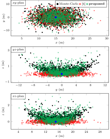
Figure 1: Comparison between uncertainty propagation models of an extended pose. An IMU moves from origin to the right at constant translational speed during $10\text{\,}\mathrm{s}$ and stops at the blue dot (15, 0, 0). We preintegrate noisy IMU measurements in a factor and generate a dispersion of the factor belief at the end-point. The true dispersion (black dots) is based on Monte-Carlo using the actual IMU noise model, green dots are generated through the proposed uncertainty model and red dots are generated using state-of-the-art [6]. The true distribution is curved in $xz$- and $yz$-planes, and only the proposed scheme captures this effect and agrees with true dispersion.

When one uses an IMU, a sensor that embeds gyrometers and accelerometers, one manipulates the pose of the sensor and its velocity that we refer in this paper to as an extended pose. An extended pose cannot be modeled as an element of $SE(3)$. As a result, the IMU propagation equations are not amenable to the framework of [5, 4].

Besides, the theory of IMU preintegration [6, 7] allows defining a unique factor between two keyframes from a sequence of inertial measurements, independently from the current estimate. In this field “it is of paramount importance to accurately model the noise covariance [of the preintegrated factor]” [6], i.e. the factor belief. Figure 1 illustrates how the uncertainty representation of an extended pose advocated in this paper correctly computes the underlying factor belief.

In this work, which is an extension of preliminary results [8], we define 5$\times$5 matrices to model extended poses, and show how our approach allows transposing the framework dealing with the Lie group approach to pose uncertainty to the context of IMUs. Our contributions are as follows:

1. we show how to propagate uncertainty of an extended pose through the IMU kinematic model, where we provide a substantial extension of the results of [5] to position, orientation plus velocity when using IMUs;

2. we address IMU preintegration. This paper provides a theoretical framework for preintegrating IMU on the Lie group of extended poses. It notably simplifies and improves the preintegration on manifold [6], provides a rigorous treatment of Coriolis force, and handles IMU biases slightly more accurately than the approach of [6];

3. we numerically demonstrate the efficiency of our theoretical framework through massive simulations and real experiments;

4. we implement a loosely-coupled approach based on iSAM2 [9] that obtains reliable estimates for one hour long sequences acquired with our car equipped with an IMU, and a LiDAR that outputs relative translations;

5. an accompanying set of Python scripts to implement many of the key equations and regenerate the plots in the paper, and our GTSAM fork, are downloadable from https://github.com/mbrossar/SE2-3-;

6. the supplementary material that accompanies the present paper contains detailed proofs along with comprehensive technical derivations.

I-A Relations with $SE(3)$ based Uncertainty Propagation

One contribution of [4], and [5] also, consists in compounding pose uncertainties based on a discrete-time integration of the $SE(3)$ kinematic equation as

$$\mathbf{T}_{i+1}=\mathbf{T}_{i}\boldsymbol{\Upsilon}_{i},$$ (1)

where $\mathbf{T}_{i}$ is a global pose and $\boldsymbol{\Upsilon}_{i}$ is a local increment, a scheme which is not applicable to IMU kinematic equations. We generalize (1) and propagate an extended pose as

$$\mathbf{T}_{i+1}=\boldsymbol{\Gamma}_{i}\Phi(\mathbf{T}_{i})\boldsymbol{\Upsilon}_{i},$$ (2)

where $\mathbf{T}_{i}$ is a global extended pose, $\boldsymbol{\Gamma}_{i}$ is a global increment, $\boldsymbol{\Upsilon}_{i}$ a local increment, and $\Phi(\cdot)$ a function that depends only on the time between instants $i$ and $i+1$. The scheme (1) models a robot driving in the environment where $\boldsymbol{\Upsilon}_{i}$ is given by, e.g., differential wheel speeds or visual relative pose estimates. To derive kinematic model (2), we build on a novel representation of extended poses by 5$\times$5 matrices, namely the group $SE_{2}(3)$, introduced in the recent paper [10] for navigation.

To express how pose uncertainty evolves, [5] associates uncertainty to poses as

$$\mathbf{T}_{i}=\mathbf{\hat{T}}_{i}\exp(\boldsymbol{\xi}_{i}),\quad\boldsymbol{\Upsilon}_{i}=\hat{\boldsymbol{\Upsilon}}_{i}\exp(\boldsymbol{\eta}_{i}),$$ (3)

where $\mathbf{\hat{T}}_{i}$ and $\hat{\boldsymbol{\Upsilon}}_{i}$ are noise-free variables, $\exp(\cdot)$ is the $SE(3)$ exponential map, and $\boldsymbol{\xi}_{i}\sim\mathcal{N}(\mathbf{0}_{6},\boldsymbol{\Sigma}_{i})$ and $\boldsymbol{\eta}_{i}\sim\mathcal{N}(\mathbf{0}_{6},\mathbf{Q})$ are uncertainties, a.k.a. errors or noises. In a probabilistic context, the compound (1) is then rewritten as

$$\mathbf{\hat{T}}_{i+1}\exp(\boldsymbol{\xi}_{i+1})=\mathbf{\hat{T}}_{i}\exp(\boldsymbol{\xi}_{i})\hat{\boldsymbol{\Upsilon}}_{i}\exp(\boldsymbol{\eta}_{i}).$$ (4)

Given nominal values and associated uncertainties $\{\mathbf{\hat{T}}_{i},\boldsymbol{\Sigma}_{i}\}$, $\{\hat{\boldsymbol{\Upsilon}}_{i},\mathbf{Q}\}$, [5] shows how to compute $\{\mathbf{\hat{T}}_{i+1},\boldsymbol{\Sigma}_{i+1}\}$.

By similarly leveraging (3), we investigate in this paper how extended pose uncertainties propagate through (2) as

$$\mathbf{\hat{T}}_{i+1}\exp(\boldsymbol{\xi}_{i+1})=\boldsymbol{\Gamma}_{i}\Phi\left(\mathbf{\hat{T}}_{i}\exp(\boldsymbol{\xi}_{i})\right)\hat{\boldsymbol{\Upsilon}}_{i}\exp(\boldsymbol{\eta}_{i}),$$

where naturally $\exp(\cdot)$ denotes the exponential map of $SE_{2}(3)$, which is an extension of $SE(3)$ suited to robot state estimation involving IMUs. The obtained formulas have very concrete implications for preintegration, see Section V.

I-B Links and Differences with Existing Literature

In robotics, it is well established that estimating uncertain spatial relationships is fundamentally important for state-estimation [11, 12], robot control [13], or active SLAM [14].

The pioneering works [15, 16] notices that mobile robots dispersion under the effect of sensor noise resembles more a “banana” than a standard ellipse, which is accurately approximated with Gaussian distributions in Lie exponential coordinates of $SE(2)$ [17]. This paves the ways for defining uncertainty on manifolds, see e.g. [18, 19], and for Gaussians on $SE(3)$ [16, 18]. [4] obtained the first results about uncertainty propagation on $SE(3)$ in a general and non-parametric context, which are complemented by the results of [5] in discrete time. The approach is extended to continuous time in [20, 21, 22], and to correlated pose uncertainties in [23].

Preintegrating IMU is an alternative to the standard inertial measurement integration which has de facto been adopted in optimization-based estimation framework such as GTSAM [24] and OKVIS [25]. It was initiated by [26] and later improved in [27, 6, 7, 28] notably for avoiding singularities due to the use of Euler angles. IMU preintegration is adapted, e.g., for legged robot odometry [29, 30], differential drive motion model [31], unknown time offset [32], wheel odometry[33, 34], and covariance preintegration [35]. This paper generalizes and goes beyond the manifold representation of [6]. Indeed the latter is concerned with the manifold structure of Lie group $SO(3)$ only, and treats the remainder of the state linearly, whereas we embed the whole state into the group $SE_{2}(3)$. Beyond the “on-manifold” approach we hence also benefit from the fact the very structure of $SE_{2}(3)$ proves much more accurate for describing IMU-related equations and uncertainty propagation. The choice of the $SE_{2}(3)$ Lie group formalism takes its roots in invariant Kalman filtering, see [10, 36], which has led to more accurate and consistent extended Kalman filters and has yet prompted a high-end industrial product[37].

The work of [38], later extended in a visual-inertial navigation system in [39], introduces preintegration in its continuous form, [40] proposes asynchronous preintegration with Gaussian processes, [41] addresses continuous preintegration as a higher-order Taylor expansion, [42] describes a scheme based on switched linear systems, and [43, 44] provide closed-form expressions for computing analytically the preintegration factors. This work improves the Euler integration scheme of [6] to limit discretization errors, whose integration schemes remain compatible with our approach based on exact discretization.

This paper is an extension of our preliminary conference paper [8], see also early ideas in [45], that contains in-depth discussions, comprehensive technical derivations, numerical and real experiments, and publicly available implementation.

I-C Organization of the Paper

The remainder of the paper is organized as follows. Section II presents the mathematical tools that we use throughout the paper. Section III recaps our previous results. Section IV shows how to propagate an extended pose and its uncertainty. Section V addresses IMU preintegration on flat Earth and Section VI its extension on rotating Earth. Section VII contains real experiments demonstrating the relevance of the approach.

II Mathematical Preliminaries

To familiarize with Lie group theory for robotics, please refer to [2], or [17, 46].

II-A $SE_{2}(3)$, the Lie Group of Extended Poses

Estimating the orientation $\mathbf{R}$, velocity $\mathbf{v}$ and position $\mathbf{p}$ of a rigid body in space is a common problem in robotic navigation and perception. We represent in this paper rotation $\mathbf{R}$ with the special orthogonal group

$$SO(3):=\left\{\mathbf{R}\in\mathbb{R}^{3\times 3}~{}|~{}\mathbf{R}\mathbf{R}^{T}=\mathbf{I}_{3},~{}\det\mathbf{R}=1\right\}.$$

The set of poses may be defined using homogeneous matrices of the special Euclidean group

$$SE(3):=\left\{\mathbf{T}=\begin{bmatrix}\begin{array}[]{c|c}\mathbf{R}&\mathbf{p}\\ \hline\cr\mathbf{0}_{3}^{T}&1\end{array}\end{bmatrix}\in\mathbb{R}^{4\times 4}~{}\bigg{|}~{}\begin{matrix}\mathbf{R}\in SO(3)\\ \mathbf{p}\in\mathbb{R}^{3}\end{matrix}\right\}.$$

This paper describes extended poses through the following group first introduced to the best of our knowledge in [10]

$$SE_{2}(3):=\left\{\mathbf{T}=\begin{bmatrix}\begin{array}[]{c|cc}\mathbf{R}&\mathbf{v}&\mathbf{p}\\ \hline\cr\mathbf{0}_{2\times 3}&\lx@intercol\hfil\mathbf{I}_{2}\hfil\lx@intercol\end{array}\end{bmatrix}\in\mathbb{R}^{5\times 5}\Bigg{|}\begin{matrix}~{}\mathbf{R}\in SO(3)\\ \mathbf{v},\mathbf{p}\in\mathbb{R}^{3}\end{matrix}\right\}.$$

$SO(3)$, $SE(3)$ and $SE_{2}(3)$ are matrix Lie groups where matrix multiplication provides group composition of two elements, and matrix inverse provides element inverse. The linear operator $\wedge$ maps elements $\boldsymbol{\xi}\in\mathbb{R}^{9}$ to the Lie algebra of $SE_{2}(3)$

$$\boldsymbol{\xi}^{\wedge} :=\begin{bmatrix}\boldsymbol{\phi}\\ \boldsymbol{\nu}\\ \boldsymbol{\rho}\end{bmatrix}^{\wedge}:=\begin{bmatrix}\begin{array}[]{c|cc}\boldsymbol{\phi}_{\times}&\boldsymbol{\nu}&\boldsymbol{\rho}\\ \hline\cr\mathbf{0}_{2\times 3}&\lx@intercol\hfil\mathbf{0}_{2\times 2}\hfil\lx@intercol\end{array}\end{bmatrix}\in\mathfrak{se}_{2}(3),$$ (5)

where $\boldsymbol{\phi}\in\mathbb{R}^{3}$, $\boldsymbol{\nu}\in\mathbb{R}^{3}$, $\boldsymbol{\rho}\in\mathbb{R}^{3}$, and

$$\boldsymbol{\phi}_{\times}:=\begin{bmatrix}\phi_{1}\\ \phi_{2}\\ \phi_{3}\end{bmatrix}_{\times}:=\begin{bmatrix}0&-\phi_{3}&\phi_{2}\\ \phi_{3}&0&-\phi_{1}\\ -\phi_{2}&\phi_{1}&0\end{bmatrix}$$ (6)

denotes the skew symmetric matrix associated with cross product with $\boldsymbol{\phi}$, which maps also a 3$\times$1 vector to an element of $\mathfrak{so}(3)$, the Lie algebra of $SO(3)$.

II-A1 Exponential, Logarithm, & Adjoint Operator

the exponential map conveniently maps an element $\boldsymbol{\xi}\in\mathbb{R}^{9}$ to $SE_{2}(3)$

$$\exp(\boldsymbol{\xi}):=\exp_{m}(\boldsymbol{\xi}^{\wedge})=\sum_{k=0}^{\infty}\frac{1}{k!}\left(\boldsymbol{\xi}^{\wedge}\right)^{k},$$ (7)

and its local inverse, the logarithm map, defined as

$$\color[rgb]{0,0,0}\log(\mathbf{T}) \color[rgb]{0,0,0}=\left(\sum_{k=1}^{\infty}(-1)^{k+1}\frac{(\mathbf{T}-\mathbf{I}_{5})^{k}}{k}\right)^{\vee},$$ (8)

where $\vee$ is the inverse of $\wedge$, enables to map the small perturbation $\exp(\boldsymbol{\xi})\in SE_{2}(3)$ to $\mathbb{R}^{9}$ such that

$$\boldsymbol{\xi}=\log\big{(}\exp\left(\boldsymbol{\xi}\right)\big{)}.$$ (9)

We conveniently define the adjoint operator

$$\operatorname{Ad}_{\mathbf{T}}:=\begin{bmatrix}\mathbf{R}&\mathbf{0}_{3\times 3}&\mathbf{0}_{3\times 3}\\ \mathbf{v}_{\times}\mathbf{R}&\mathbf{R}&\mathbf{0}_{3\times 3}\\ \mathbf{p}_{\times}\mathbf{R}&\mathbf{0}_{3\times 3}&\mathbf{R}\end{bmatrix}$$ (10)

as an operator acting directly on $\mathbb{R}^{9}$. The following relations prove extremely useful:

$$\mathbf{T}\exp(\boldsymbol{\xi})\mathbf{T}^{-1} =\exp(\operatorname{Ad}_{\mathbf{T}}\boldsymbol{\xi}),$$ (11)

$$\Rightarrow\mathbf{T}\exp(\boldsymbol{\xi}) =\exp(\operatorname{Ad}_{\mathbf{T}}\boldsymbol{\xi})\mathbf{T},$$ (12)

$$\operatorname{Ad}_{\boldsymbol{\Gamma}}\operatorname{Ad}_{\mathbf{T}} =\operatorname{Ad}_{\boldsymbol{\Gamma}\mathbf{T}}.$$ (13)

II-A2 Baker-Campbell-Hausdorff (BCH) Formula

the BCH formula provides powerful tools to manipulate uncertainty on Lie groups, which can be used to compound two matrix exponentials

$$\log_{m}\big{(}\exp_{m}(\mathbf{A})\exp_{m}(\mathbf{B})\big{)}=\mathbf{A}+\mathbf{B}+\frac{1}{2}\left[\mathbf{A},\mathbf{B}\right]$$

$$+\frac{1}{12}\left(\left[\mathbf{A},\left[\mathbf{A},\mathbf{B}\right]\right]+\left[\mathbf{B},\left[\mathbf{B},\mathbf{A}\right]\right]\right)-\frac{1}{24}\left[\mathbf{B},\left[\mathbf{A},\left[\mathbf{A},\mathbf{B}\right]\right]\right]+\ldots$$

in terms of infinite series, where the Lie bracket is given by

$$[\mathbf{A},\mathbf{B}]:=\mathbf{A}\mathbf{B}-\mathbf{B}\mathbf{A}.$$

In the particular case of $SE_{2}(3)$, we have

$$[\boldsymbol{\xi}^{\wedge},\boldsymbol{\eta}^{\wedge}]:=\boldsymbol{\xi}^{\wedge}\boldsymbol{\eta}^{\wedge}-\boldsymbol{\xi}^{\wedge}\boldsymbol{\eta}^{\wedge}=\left(\boldsymbol{\xi}^{\curlywedge}\boldsymbol{\eta}\right)^{\wedge},$$ (14)

where the “curlywedge” $\curlywedge$ operator is defined as

$$\boldsymbol{\xi}^{\curlywedge}:=\begin{bmatrix}\boldsymbol{\phi}\\ \boldsymbol{\nu}\\ \boldsymbol{\rho}\end{bmatrix}^{\curlywedge}:=\begin{bmatrix}\boldsymbol{\phi}_{\times}&\mathbf{0}_{3\times 3}&\mathbf{0}_{3\times 3}\\ \boldsymbol{\nu}_{\times}&\boldsymbol{\phi}_{\times}&\mathbf{0}_{3\times 3}\\ \boldsymbol{\rho}_{\times}&\mathbf{0}_{3\times 3}&\boldsymbol{\phi}_{\times}\end{bmatrix},$$ (15)

which is 9$\times$9. We note that

$$\log\big{(}\exp\left(\boldsymbol{\xi}\right)\exp\left(\boldsymbol{\eta}\right)\big{)}=\boldsymbol{\xi}+\boldsymbol{\eta}+\frac{1}{2}\boldsymbol{\xi}^{\curlywedge}\boldsymbol{\eta}$$

$$+\frac{1}{12}\left(\boldsymbol{\xi}^{\curlywedge}\boldsymbol{\xi}^{\curlywedge}\boldsymbol{\eta}+\boldsymbol{\eta}^{\curlywedge}\boldsymbol{\eta}^{\curlywedge}\boldsymbol{\xi}\right)-\frac{1}{24}\boldsymbol{\eta}^{\curlywedge}\boldsymbol{\xi}^{\curlywedge}\boldsymbol{\xi}^{\curlywedge}\boldsymbol{\eta}+\ldots,$$ (16)

showing $\exp(\boldsymbol{\xi})\exp(\boldsymbol{\eta})\neq\exp(\boldsymbol{\xi}+\boldsymbol{\eta})$. We thus require approximations to compute the logarithm of a product of exponentials. If we assume, e.g., that $\boldsymbol{\eta}$ is a small noise while $\boldsymbol{\xi}$ is non-negligible, we get

$$\log\big{(}\exp\left(\boldsymbol{\xi}\right)\exp\left(\boldsymbol{\eta}\right)\big{)}=\boldsymbol{\xi}+\mathbf{\mathcal{J}}^{-1}_{\boldsymbol{\xi}}\boldsymbol{\eta}+O(\|\boldsymbol{\eta}\|^{2}),$$ (17)

where $\mathbf{\mathcal{J}}^{-1}_{\boldsymbol{\xi}}$ is the 9$\times$9 inverse left-Jacobian of $SE_{2}(3)$. If both $\boldsymbol{\xi}$ and $\boldsymbol{\eta}$ are small quantities, we recover the first-order approximation

$$\log\big{(}\exp\left(\boldsymbol{\xi}\right)\exp\left(\boldsymbol{\eta}\right)\big{)} =\boldsymbol{\xi}+\boldsymbol{\eta}+O(\|\boldsymbol{\xi}\|^{2},\|\boldsymbol{\eta}\|^{2}).$$ (18)

Closed-form expressions of $\exp(\cdot)$, $\log(\cdot)$ and Jacobians are given in Appendix.

Remark 1 (Overloading Operators).

We overload the $\exp(\cdot)$, $\log(\cdot)$, and Jacobian in the sense that they can be applied to both 3$\times$1 and 9$\times$1 vectors for respectively $SO(3)$ and $SE_{2}(3)$ exponential, logarithm and Jacobian.

II-B Uncertainty & Random Variables on $SE_{2}(3)$

Let $\mathbf{\hat{T}}\in SE_{2}(3)$ represent a noise-free value, and $\boldsymbol{\xi}\in\mathbb{R}^{9}$ a small perturbation. The approach based on additive uncertainty “$\mathbf{\hat{T}}+\boldsymbol{\xi}$” is not valid as these quantities are not vector elements. In contrast, we define a random variable on $SE_{2}(3)$

$$\mathbf{T}:=\mathbf{\hat{T}}\exp(\boldsymbol{\xi}),$$ (19)

where $\mathbf{\hat{T}}$ is a noise-free “mean” of the distribution and $\boldsymbol{\xi}\sim\mathcal{N}(\mathbf{0}_{9},\boldsymbol{\Sigma})$ is a zero-mean multivariate Gaussian in $\mathbb{R}^{9}$. We thus describe statistical dispersion of extended poses with the exponential map. This approach is referred to as “concentrated Gaussian” [47, 18], and has been largely advocated for Lie groups, see [36, 10, 48, 5].

Remark 2 (Left and Right Perturbations).

We apply perturbations in (19) on the right rather than the left as in [5]. Both are valid, right perturbations are more convenient to propagate extended pose uncertainties in the context of this paper, and one can move from right perturbations to left perturbations and vice-versa through the relation (12).

III IMU Equations on Flat Earth Revisited

This section presents the IMU kinematic model on flat Earth (e.g. with an inertial frame of reference) and transposes it into the form (2). This was introduced in the bias- and noise-free case in [45], see proofs therein. Noises, biases and rotating Earth are progressively addressed in the following sections.

III-A IMU Kinematic Equations on Flat Earth

Let $\mathbf{R}$ denote the rotation matrix encoding the orientation of the IMU, i.e. the rotation from the global frame to the local inertial frame, and let $\mathbf{v}$ and $\mathbf{p}$ denote the velocity and the position of the IMU expressed in the global frame. An IMU collects angular velocity $\boldsymbol{\omega}^{m}$ and proper acceleration $\mathbf{a}^{m}$ measurements which relate to the corresponding true values $\boldsymbol{\omega}$ and $\mathbf{a}$ as

$$\boldsymbol{\omega}^{m} =\boldsymbol{\omega}+\mathbf{b}^{\boldsymbol{\omega}}+\boldsymbol{\eta}^{\boldsymbol{\omega}},$$ (20)

$$\mathbf{a}^{m} =\mathbf{a}+\mathbf{b}^{\mathbf{a}}+\boldsymbol{\eta}^{\mathbf{a}}.$$ (21)

The measurements are corrupted both by the time-varying biases $\mathbf{b}^{\boldsymbol{\omega}}$ and $\mathbf{b}^{\mathbf{a}}$, and zero-mean white Gaussian noises $\boldsymbol{\eta}^{\boldsymbol{\omega}}$ and $\boldsymbol{\eta}^{\mathbf{a}}$. The motion equations of the IMU sensor on flat Earth write

$$\dot{\mathbf{R}} =\mathbf{R}\left(\boldsymbol{\omega}^{m}-\mathbf{b}^{\boldsymbol{\omega}}-\boldsymbol{\eta}^{\boldsymbol{\omega}}\right)_{\times},$$ (22)

$$\dot{\mathbf{v}} =\mathbf{R}\left(\mathbf{a}^{m}-\mathbf{b}^{\mathbf{a}}-\boldsymbol{\eta}^{\mathbf{a}}\right)+\mathbf{g},$$ (23)

$$\dot{\mathbf{p}} =\mathbf{v},$$ (24)

where $\mathbf{g}=[0~{}0~{}-9.81]^{T}\in\mathbb{R}^{3}$ is the global gravity vector.

III-B Revisiting IMU Equations for Extended Poses

Following [45], we may rewrite the model (22)-(24) in the form (2) as follows. First, we associate a matrix $\mathbf{T}_{t}\in SE_{2}(3)$ to the extended pose $\{\mathbf{R},\mathbf{v},\mathbf{p}\}$ at time $t$. Then, we write $\mathbf{T}_{0}$ the solution initialized at $t_{0}=0$, such that

$$\mathbf{T}_{t}=\boldsymbol{\Gamma}_{t}\Phi_{t}(\mathbf{T}_{0})\boldsymbol{\Upsilon}_{t},$$ (25)

where $\Phi_{t}(\cdot)$ and $\boldsymbol{\Gamma}_{t}$ only depend on $t$ as

$$\Phi_{t}(\mathbf{T}) :=\begin{bmatrix}\begin{array}[]{c|cc}\mathbf{R}&\lx@intercol\hfil\mathbf{v}\hfil\lx@intercol\vrule\lx@intercol&\mathbf{p}+t\mathbf{v}\\ \hline\cr\mathbf{0}_{2\times 3}&\lx@intercol\hfil\mathbf{I}_{2}\hfil\lx@intercol\end{array}\end{bmatrix},$$ (26)

$$\boldsymbol{\Gamma}_{t} :=\begin{bmatrix}\begin{array}[]{c|cc}\mathbf{I}_{3}&\lx@intercol\hfil t\mathbf{g}\hfil\lx@intercol\vrule\lx@intercol&\mathbf{g}t^{2}/2\\ \hline\cr\mathbf{0}_{2\times 3}&\lx@intercol\hfil\mathbf{I}_{2}\hfil\lx@intercol\end{array}\end{bmatrix},$$ (27)

and where $\boldsymbol{\Upsilon}_{t}$ is solution to differential equations leading to

$$\boldsymbol{\Upsilon}_{t}:=\begin{bmatrix}\begin{array}[]{c|cc}\Delta\mathbf{R}_{t}&\Delta\mathbf{v}_{t}&\Delta\mathbf{p}_{t}\\ \hline\cr\mathbf{0}_{2\times 3}&\lx@intercol\hfil\mathbf{I}_{2}\hfil\lx@intercol\end{array}\end{bmatrix},$$ (28)

where

$$\Delta\mathbf{R}_{t} =\exp\bigg{(}\int_{0}^{t}\boldsymbol{\omega}dt\bigg{)}=\exp\bigg{(}\int_{0}^{t}\left(\boldsymbol{\omega}^{m}-\mathbf{b}^{\boldsymbol{\omega}}-\boldsymbol{\eta}^{\boldsymbol{\omega}}\right)dt\bigg{)},$$ (29)

$$\Delta\mathbf{v}_{t} =\int_{0}^{t}\Delta\mathbf{R}_{t}\mathbf{a}dt=\int_{0}^{t}\Delta\mathbf{R}_{t}\left(\mathbf{a}^{m}-\mathbf{b}^{\mathbf{a}}-\boldsymbol{\eta}^{\mathbf{a}}\right)dt,$$ (30)

$$\Delta\mathbf{p}_{t} =\int_{0}^{t}\Delta\mathbf{v}_{t}dt.$$ (31)

The reader can check differentiating the product (25) and using (26)-(28) that we recover (22)-(24). $\Delta\mathbf{R}_{t}$, $\Delta\mathbf{v}_{t}$ and $\Delta\mathbf{p}_{t}$, referred to as the preintegrated measurements in [6], are quantities based solely on the inertial measurements and do not depend on the initial state $\mathbf{T}_{0}$. This allows to define a unique factor between extended poses at arbitrary temporally distant keyframes based on a unique integration of IMU outputs.

We now consider discrete time steps with time interval $\Delta t$. Denoting $\boldsymbol{\Gamma}_{i}:=\boldsymbol{\Gamma}_{\Delta t}$, $\Phi:=\Phi_{\Delta t}$, and $\boldsymbol{\Upsilon}_{i}:=\boldsymbol{\Upsilon}_{\Delta t}$ we get

$$\mathbf{T}_{i+1}=\boldsymbol{\Gamma}_{i}\Phi(\mathbf{T}_{i})\boldsymbol{\Upsilon}_{i},$$ (32)

where $\boldsymbol{\Gamma}_{i}$, $\mathbf{T}_{i}$, and $\boldsymbol{\Upsilon}_{i}$ all live in $SE_{2}(3)$. The reader may readily check that $\Phi(\boldsymbol{\Gamma}\mathbf{T})=\Phi(\boldsymbol{\Gamma})\Phi(\mathbf{T})$ and $\Phi\left(\exp\left(\boldsymbol{\xi}\right)\right)=\exp(\mathbf{F}\boldsymbol{\xi})$, that we combine as

$$\Phi\big{(}\mathbf{T}\exp(\boldsymbol{\xi})\big{)}=\Phi\left(\mathbf{T}\right)\exp\left(\mathbf{F}\boldsymbol{\xi}\right),$$ (33)

where

$$\mathbf{F}:=\mathbf{F}_{\Delta t}:=\begin{bmatrix}\mathbf{I}_{3}&\mathbf{0}_{3\times 3}&\mathbf{0}_{3\times 3}\\ \mathbf{0}_{3\times 3}&\mathbf{I}_{3}&\mathbf{0}_{3\times 3}\\ \mathbf{0}_{3\times 3}&\Delta t\mathbf{I}_{3}&\mathbf{I}_{3}\end{bmatrix}.$$ (34)

Remark 3 (Exact Discretization).

The formula (32) is an exact discretization of (22)-(24). However it involves (29)-(31) that need to be numerically solved at some point. As IMU measurements come in discrete-time at a high rate, we may call $\Delta t$ the discretization step, assume measurements to be constant over time intervals $\Delta t$, and perform Euler, midpoint, or more sophisticated integration schemes [44, 38, 42, 6].

III-C Noise Model and Approximation

An IMU actually measures noisy observations (20)-(21) and we consider IMU noise in the form of

$$\boldsymbol{\Upsilon}_{i}:=\hat{\boldsymbol{\Upsilon}}_{i}\exp(\boldsymbol{\eta}_{i}),\quad\boldsymbol{\eta}_{i}\sim\mathcal{N}(\mathbf{0}_{9},\mathbf{Q}),$$ (35)

where $\boldsymbol{\Upsilon}_{i}$ refers to the true quantity and $\hat{\boldsymbol{\Upsilon}}_{i}=\hat{\boldsymbol{\Upsilon}}_{i}(\hat{\mathbf{b}}_{i})$ refers to the estimated one that has been computed with estimated biases

$$\hat{\mathbf{b}}_{i}:=\begin{bmatrix}\hat{\mathbf{b}}^{\boldsymbol{\omega}}_{i}\\ \hat{\mathbf{b}}^{\mathbf{a}}_{i}\end{bmatrix}.$$ (36)

To justify (35), let us integrate IMU kinematics (22)-(24) for one time step with constant global acceleration:

$$\hat{\boldsymbol{\Upsilon}}_{i}=\begin{bmatrix}\begin{array}[]{c|cc}\exp(\hat{\boldsymbol{\omega}}_{i}\Delta t)&\hat{\mathbf{a}}_{i}\Delta t&\hat{\mathbf{a}}_{i}\Delta t^{2}/2\\ \hline\cr\mathbf{0}_{2\times 3}&\lx@intercol\hfil\mathbf{I}_{2}\hfil\lx@intercol\end{array}\end{bmatrix},$$ (37)

where $\hat{\boldsymbol{\omega}}_{i}=\boldsymbol{\omega}^{m}_{i}-\hat{\mathbf{b}}_{i}^{\boldsymbol{\omega}}$ and $\hat{\mathbf{a}}_{i}=\mathbf{a}^{m}_{i}-\hat{\mathbf{b}}_{i}^{\mathbf{a}}$. This leads to the first-order in the noise terms to

$$\boldsymbol{\Upsilon}_{i}\stackrel{{\scriptstyle\eqref{eq:bch1}}}{{=}}\hat{\boldsymbol{\Upsilon}}_{i}\exp\Big{(}\underbrace{\mathbf{G}_{i}\begin{bmatrix}\boldsymbol{\eta}^{\boldsymbol{\omega}}_{i}\\ \boldsymbol{\eta}^{\mathbf{a}}_{i}\end{bmatrix}}_{\boldsymbol{\eta}_{i}}+O(\|\boldsymbol{\eta}_{i}\|^{2})\Big{)},$$ (38)

where we define the 9$\times$6 matrix

$$\mathbf{G}_{i}=-\begin{bmatrix}\mathbf{\mathcal{J}}_{\hat{\boldsymbol{\omega}}_{i}\Delta t}^{-1}\Delta t&\mathbf{0}_{3\times 3}\\ \mathbf{0}_{3\times 3}&\exp(-\hat{\boldsymbol{\omega}}_{i}\Delta t)\Delta t\\ \mathbf{0}_{3\times 3}&\exp(-\hat{\boldsymbol{\omega}}_{i}\Delta t)\Delta t^{2}/2\end{bmatrix},$$ (39)

such that the zero-mean noise $\boldsymbol{\eta}_{i}$ has covariance

$$\mathbf{Q}_{i}=\mathbf{G}_{i}\operatorname{cov}\left(\begin{bmatrix}\boldsymbol{\eta}^{\boldsymbol{\omega}}_{i}\\ \boldsymbol{\eta}^{\mathbf{a}}_{i}\end{bmatrix}\right)\mathbf{G}_{i}^{T},$$ (40)

where it is not necessary to assume that IMU noises are isotropic. We fix $\mathbf{Q}_{i}=\mathbf{Q}$ through this paper instead of defining a time varying $\mathbf{Q}_{i}$ for convenience of exposition.

Remark 4 (Bias Error).

As in [6], we start assuming in (35) that biases are known. We then investigate how an estimated bias update affects $\hat{\boldsymbol{\Upsilon}}_{i}$ in Section V-D.

Remark 5 (Integration Scheme).

We assume in (37) piecewise constant global acceleration as in [6] for convenience of exposition. Opting for a different integration scheme, e.g., with constant local acceleration [44], would modify the values inside (37) and (39) and leave the rest of paper unchanged (details are given in the supplementary material). There also exists polynomial structures for higher order uncertainty tracking [49], see and [50] for discussions in the Gaussian context.

IV Propagating Uncertainty of Extended Poses

The goal of the present section is to compute uncertainty of an extended pose given an initial uncertainty and IMU noises.

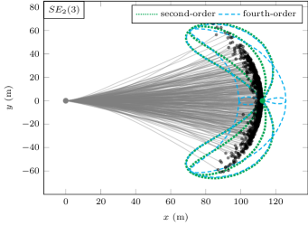
Figure 2: Example of propagation of an extended pose with $SE_{2}(3)$ uncertainty representation. The green (second-order) and cyan (fourth-order) lines are the principal great circles of the $3\sigma$ covariance ellipsoid, given by $\boldsymbol{\Sigma}_{K}$, mapped to the $xy$-plane. Looking at the area around the green dot (112.5, 0), corresponding to straight ahead and noise-free model, the fourth-order scheme has some nonzero uncertainty similarly to the Monte-Carlo samples (black dots), whereas the second-order scheme does not. The small cyan lemniscate around (112.5, 0) corresponds to a great circle of the fourth-order distribution which is absent in the second-order one.

IV-A Propagating Uncertainty through Noise-Free IMU Model

Let

$$\mathbf{T}_{i}:=\mathbf{\hat{T}}_{i}\exp(\boldsymbol{\xi}_{i}),\quad\boldsymbol{\xi}_{i}\sim\mathcal{N}(\mathbf{0}_{9},\boldsymbol{\Sigma}_{i}),$$ (41)

be our extended pose estimate with error $\boldsymbol{\xi}_{i}$. The propagation of $\mathbf{T}_{i}$ through noise-free model (32) writes

$$\mathbf{T}_{i+1} \stackrel{{\scriptstyle\eqref{eq:com_ext_pos2}}}{{=}}\boldsymbol{\Gamma}_{i}\Phi(\mathbf{T}_{i})\hat{\boldsymbol{\Upsilon}}_{i}\stackrel{{\scriptstyle\eqref{eq:initnoise}}}{{=}}\boldsymbol{\Gamma}_{i}\Phi\big{(}\mathbf{\hat{T}}_{i}\exp(\boldsymbol{\xi}_{i})\big{)}\hat{\boldsymbol{\Upsilon}}_{i}$$

$$\stackrel{{\scriptstyle\eqref{eq:phiprop}}}{{=}}\boldsymbol{\Gamma}_{i}\Phi(\mathbf{\hat{T}}_{i})\Phi\big{(}\mathbf{F}\exp(\boldsymbol{\xi}_{i})\big{)}\hat{\boldsymbol{\Upsilon}}_{i}$$

$$\stackrel{{\scriptstyle\eqref{eq:adjoint2}}}{{=}}\underbrace{\boldsymbol{\Gamma}_{i}\Phi(\mathbf{\hat{T}}_{i})\hat{\boldsymbol{\Upsilon}}_{i}}_{\mathbf{\hat{T}}_{i+1}}\exp(\underbrace{\operatorname{Ad}_{\hat{\boldsymbol{\Upsilon}}_{i}^{-1}}\mathbf{F}\boldsymbol{\xi}_{i}}_{\boldsymbol{\xi}_{i+1}}).$$ (42)

By defining the new mean $\mathbf{\hat{T}}_{i+1}$, the covariance of the discrepancy evolves without approximation as

$$\boldsymbol{\Sigma}_{i+1}:=\operatorname{E}[\boldsymbol{\xi}_{i+1}\boldsymbol{\xi}_{i+1}^{T}] \stackrel{{\scriptstyle\eqref{eq:mean1}}}{{=}}\underbrace{\operatorname{Ad}_{\hat{\boldsymbol{\Upsilon}}_{i}^{-1}}\mathbf{F}}_{:=\mathbf{A}_{i}}\boldsymbol{\Sigma}_{i}\left(\operatorname{Ad}_{\hat{\boldsymbol{\Upsilon}}_{i}^{-1}}\mathbf{F}\right)^{T}.$$ (43)

This is remarkable as it proves that IMU noise-free equations, albeit nonlinear, preserve concentrated Gaussians on $SE_{2}(3)$ and the moments evolve through closed-form formulas.

IV-B Propagating Uncertainty through Noisy IMU Model

We now consider IMU noise in the form of (35). Our Lie group approach to extended poses allows transposing the developments of [5] exposed for the evolution model (4). The propagation of $\mathbf{T}_{i}$ through noisy model writes

$$\mathbf{T}_{i+1}=\underbrace{\boldsymbol{\Gamma}_{i}\Phi(\mathbf{\hat{T}}_{i})\hat{\boldsymbol{\Upsilon}}_{i}}_{\mathbf{\hat{T}}_{i+1}}\exp(\underbrace{\operatorname{Ad}_{\hat{\boldsymbol{\Upsilon}}_{i}^{-1}}\mathbf{F}\boldsymbol{\xi}_{i}}_{\boldsymbol{\xi}})\exp\left(\boldsymbol{\eta}_{i}\right),$$ (44)

where we recover (42) with noise injected on the right. For our approach to hold, we require that $\operatorname{E}[\boldsymbol{\xi}_{i+1}]=\mathbf{0}_{9}$, where

$$\boldsymbol{\xi}_{i+1} \stackrel{{\scriptstyle\eqref{eq:initnoise}}}{{=}}\log(\mathbf{\hat{T}}_{i+1}^{-1}\mathbf{T}_{i+1})$$

$$\stackrel{{\scriptstyle\eqref{eq:mean}}}{{=}}\log\big{(}\exp\left(\boldsymbol{\xi}\right)\exp\left(\boldsymbol{\eta}_{i}\right)\big{)}.$$ (45)

Applying the BCH formula (16), we get

$$\boldsymbol{\xi}_{i+1} =\boldsymbol{\xi}+\boldsymbol{\eta}_{i}+\frac{1}{2}\boldsymbol{\xi}^{\curlywedge}\boldsymbol{\eta}_{i}+\frac{1}{12}\big{(}\boldsymbol{\xi}^{\curlywedge}\boldsymbol{\xi}^{\curlywedge}\boldsymbol{\eta}_{i}+\boldsymbol{\eta}_{i}^{\curlywedge}\boldsymbol{\eta}_{i}^{\curlywedge}\boldsymbol{\xi}\big{)}$$

$$~{}~{}-\frac{1}{24}\boldsymbol{\eta}_{i}^{\curlywedge}\boldsymbol{\xi}^{\curlywedge}\boldsymbol{\xi}^{\curlywedge}\boldsymbol{\eta}_{i}+O(\|\boldsymbol{\xi}_{i+1}\|^{5})$$ (46)

As $\boldsymbol{\xi}$ and $\boldsymbol{\eta}_{i}$ are uncorrelated, we have

$$\operatorname{E}[\boldsymbol{\xi}_{i+1}]=-\frac{1}{24}\boldsymbol{\eta}_{i}^{\curlywedge}\boldsymbol{\xi}^{\curlywedge}\boldsymbol{\xi}^{\curlywedge}\boldsymbol{\eta}_{i}+O(\|\boldsymbol{\xi}_{i+1}\|^{6})$$ (47)

since everything except the fourth-order term has zero mean. In the present paper we use “fourth-order” in the sense of [5] but it is important to note it corresponds to “second-order” in the original terminology of [4]. Thus, to third-order, we can safely assume that $\operatorname{E}[\boldsymbol{\xi}_{i+1}]=\mathbf{0}_{9}$, and thus, $\mathbf{\hat{T}}_{i+1}$ seems to be a reasonable way to compound the mean. Our goal is now to compute an approximation of $\boldsymbol{\Sigma}_{i+1}$. Multiplying out $\operatorname{E}[\boldsymbol{\xi}_{i+1}\boldsymbol{\xi}_{i+1}^{T}]$ to fourth-order (second-order in the sense of [4]), the resulting covariance is then

$$\boldsymbol{\Sigma}_{i+1}\simeq\mathbf{A}_{i}\boldsymbol{\Sigma}_{i}\mathbf{A}_{i}^{T}+\mathbf{Q}+\mathbf{S}_{\text{4th}},$$ (48)

where $\mathbf{A}_{i}$ is defined in (43), $\mathbf{Q}$ is the input noise covariance, and $\mathbf{S}_{\text{4th}}$ is the third- and fourth-order corrections to allow (48) to be correct to the fourth-order, see Appendix for its expression. This result is essentially the same as [4, 5] but worked out for the time time-varying model (32) which is more complex than (4). In summary, to propagate an extended pose, we compute the mean using (44) and the covariance using (48).

IV-C Simple Propagation Example

This subsection presents a simple example of extended pose propagation. This can be viewed as a discrete-time integration of the IMU kinematic equations (22)-(24) with biases absent or perfectly known. To see the qualitative difference between the proposed second- and fourth-order methods, respectively without and with $\mathbf{S}_{\text{4th}}$, let us propagate an extended pose many times in a row. We apply (32) for $i=0,\ldots,K-1$ with acceleration about the $x$-axis and rotational noise about the $z$-axis as

$$\mathbf{\hat{T}}_{0} =\mathbf{I}_{5},~{}~{}\boldsymbol{\xi}_{0}\sim\mathcal{N}(\mathbf{0}_{9},\mathbf{0}_{9\times 9}),$$

$$\operatorname{cov}(\boldsymbol{\eta}^{\boldsymbol{\omega}}_{i}) =\operatorname{diag}(0,0,\sigma^{2}),~{}~{}~{}\operatorname{cov}(\boldsymbol{\eta}^{\mathbf{a}}_{i})=\mathbf{0}_{3\times 3},$$

$$\hat{\boldsymbol{\Upsilon}}_{i} =\begin{bmatrix}\begin{array}[]{c|cc}\mathbf{I}_{3}&\bar{\mathbf{a}}\Delta t&\bar{\mathbf{a}}\Delta t^{2}/2\\ \hline\cr\mathbf{0}_{2\times 3}&\lx@intercol\hfil\mathbf{I}_{2}\hfil\lx@intercol\end{array}\end{bmatrix},\bar{\mathbf{a}}=\begin{bmatrix}a\\ 0\\ 9.81\end{bmatrix}-\mathbf{g}.$$

This models a robot driving in the plane with a constant translational acceleration and slightly uncertain rotational speed. We are interested in how the covariance matrix fills in over time. According to the second-order scheme, we have

$$\mathbf{\hat{T}}_{K} =\begin{bmatrix}\begin{array}[]{c|cc}&Ka\Delta t&K^{2}a^{2}\Delta t^{2}/2\\ \mathbf{I}_{3}&0&0\\ &0&0\\ \hline\cr\mathbf{0}_{3}^{T}&\lx@intercol\hfil\mathbf{I}_{2}\hfil\lx@intercol\end{array}\end{bmatrix},$$

$$\boldsymbol{\Sigma}_{K} =\begin{bmatrix}\begin{array}[]{ccc|ccc|ccc}0&0&0&0&0&0&0&0&0\\ 0&0&0&0&0&0&0&0&0\\ 0&0&1&0&\Sigma_{\phi v}&0&0&\Sigma_{\phi p}&0\\ \hline\cr 0&0&0&0&0&0&0&0&0\\ 0&0&\Sigma_{\phi v}&0&\Sigma_{vv}&0&0&\Sigma_{vp}&0\\ 0&0&0&0&0&0&0&0&0\\ \hline\cr 0&0&0&0&0&0&\underline{0}&0&0\\ 0&0&\Sigma_{\phi p}&0&\Sigma_{vp}&0&0&\Sigma_{pp}&0\\ 0&0&0&0&0&0&0&0&0\end{array}\end{bmatrix}K\sigma^{2},$$

where

$$\Sigma_{\phi v} =-\frac{\left(K-1\right)}{2}a\Delta t,$$

$$\Sigma_{\phi p} =\frac{\left(K-1\right)\left(2K-1\right)}{12}a\Delta t^{2},$$

$$\Sigma_{vv} =\frac{\left(K-1\right)\left(2K-1\right)}{6}a^{2}\Delta t^{2},$$

$$\Sigma_{vp} =\frac{\left(K-1\right)^{2}K}{8}a^{2}\Delta t^{3},$$

$$\Sigma_{pp} =\frac{\left(K-1\right)\left(2K-1\right)\left(3\left(K-1\right)^{2}+3K-4\right)}{120}a^{2}\Delta t^{4}.$$

We see that the entry of $\boldsymbol{\Sigma}_{K}$ corresponding to uncertainty in the $x$-direction (underlined zero just left above $\Sigma_{pp}$), does not grow. However, in the fourth-order scheme, the fill-in pattern is such that this entry is nonzero. This leaking of uncertainty into an additional degree of freedom cannot be captured by keeping only the second-order terms. Figure 2 provides a numerical example of this effect, where we set $K=300$, $dt=$0.05\text{\,}\mathrm{s}$$, $a=$1\text{\,}\mathrm{m}\mathrm{/}\mathrm{s}^{2}$$ and $\sigma=$0.03\text{\,}\mathrm{r}\mathrm{a}\mathrm{d}\mathrm{/}\mathrm{s}$$. It shows that:

1. both the second- and fourth-order schemes capture the actual “banana”-shaped distribution over extended poses of the Monte-Carlo samples. This is owed to the use of the exponential of $SE_{2}(3)$;

2. the fourth-order scheme has some finite uncertainty in the straight-ahead direction (the gray dot to the green dot) similarly to the sampled trajectories, while the second-order scheme does not;

3. the samples never cross a circle of radius $112.5\text{\,}\mathrm{m}$, as rotation uncertainty tends to reduce the travelled distance, and none of the approximate methods perfectly models this non-Gaussian behavior.

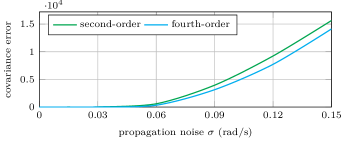
Figure 3: Error in computing covariance using second- and fourth-order methods for propagating an extended pose, as compared to Monte-Carlo. The input noise is gradually scaled up, highlighting the improved performance of the fourth-order method.

$SO(3)\times\mathbb{R}^{6}$ [6]

$$\mathbf{T} =\mathbf{\hat{T}}\boxplus\boldsymbol{\xi}$$

$$=\begin{bmatrix}\begin{array}[]{c|cc}\hat{\mathbf{R}}\exp(\boldsymbol{\phi})&\hat{\mathbf{v}}+\boldsymbol{\nu}&\hat{\mathbf{p}}+\hat{\mathbf{R}}\boldsymbol{\rho}\\ \hline\cr\mathbf{0}_{2\times 3}&\lx@intercol\hfil\mathbf{I}_{2}\hfil\lx@intercol\end{array}\end{bmatrix}$$

$$\boldsymbol{\xi} =\mathbf{T}\boxminus\mathbf{\hat{T}}=\begin{bmatrix}\log(\hat{\mathbf{R}}^{T}\mathbf{R})\\ \mathbf{v}-\hat{\mathbf{v}}\\ \hat{\mathbf{R}}^{T}(\mathbf{p}-\hat{\mathbf{p}})\end{bmatrix}$$

$SE_{2}(3)$

$$\mathbf{T} =\mathbf{\hat{T}}\exp(\boldsymbol{\xi})$$

$$=\begin{bmatrix}\begin{array}[]{c|c|c}\hat{\mathbf{R}}\exp(\boldsymbol{\phi})&\hat{\mathbf{v}}+\mathbf{\mathcal{J}}_{\boldsymbol{\phi}}\boldsymbol{\nu}&\hat{\mathbf{p}}+\mathbf{\mathcal{J}}_{\boldsymbol{\phi}}\boldsymbol{\rho}\\ \hline\cr\mathbf{0}_{2\times 3}&\lx@intercol\hfil\mathbf{I}_{2}\hfil\lx@intercol\end{array}\end{bmatrix}$$

$$\boldsymbol{\xi} =\log(\mathbf{\hat{T}}^{-1}\mathbf{T})$$

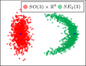
Figure 4: Comparison between the retraction and its inverse used in the preintegration on manifold [6] (left), and the ones based on $SE_{2}(3)$ exponential advocated in the present paper (center, detailed formulas are given in Appendix). On the right, the $SE_{2}(3)$ distribution (green dots) is curved whereas the $SO(3)\times\mathbb{R}^{6}$ one (red dots) is limited to ellipses. The blue points show the mean estimate.

IV-C1 Comparison with $SE_{2}(3)$ Monte-Carlo Distribution

assuming the actual distribution to be a concentrated Gaussian on $SE_{2}(3)$, the Monte-Carlo estimate of its covariance reads

$$\boldsymbol{\Sigma}_{\mathrm{mc}} :=\operatorname{E}\left[\log(\mathbf{\hat{T}}_{K}^{-1}\mathbf{T}_{K})\log(\mathbf{\hat{T}}_{K}^{-1}\mathbf{T}_{K})^{T}\right]$$

$$\simeq\frac{1}{N-1}\sum_{n=1}^{N}\log(\mathbf{\hat{T}}_{K}^{-1}\mathbf{T}_{K,n})\log(\mathbf{\hat{T}}_{K}^{-1}\mathbf{T}_{K,n})^{T}.$$

By letting $N=${10}^{6}$$ this provides a benchmark to compare the covariance matrices computed with second-order accuracy and fourth-order accuracy based on the Frobenius norm [5]

$$\text{cov. err.}:=\sqrt{\operatorname{trace}\left(\left(\boldsymbol{\Sigma}_{i\text{-th}}-\boldsymbol{\Sigma}_{\mathrm{mc}}\right)^{T}\left(\boldsymbol{\Sigma}_{i\text{-th}}-\boldsymbol{\Sigma}_{\mathrm{mc}}\right)\right)}.$$

Results are displayed in Figure 3. We see the fourth-order is a slightly better. All methods degrade as magnitude of noise increases and fourth-order is the closest to the true covariance.

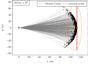
Figure 5: Same example as Figure 2 adapted to the $SO(3)\times\mathbb{R}^{6}$ uncertainty representation. The mean and the $3\sigma$ covariance ellipse relative to the Monte-Carlo distribution (orange) are fitted to the black samples to show what keeping $xy$-covariance relative to the start looks like. The red line is the $3\sigma$ ellipsoid when incrementally computing the covariance with second-order accuracy, which wrongly reveals null uncertainty in the $x$-direction. The position mean of the samples (orange dot) differs from the noise-free mean (red dot).

IV-C2 Comparison with $SO(3)\times\mathbb{R}^{6}$ Monte-Carlo Distribution

we compare the $SE_{2}(3)$ uncertainty representation to the gold-standard $SO(3)\times\mathbb{R}^{6}$ distribution used in [6] for preintegration, see Section V. This distribution defines uncertainty as

$$\mathbf{T} :=\mathbf{\hat{T}}\boxplus\boldsymbol{\xi},~{}~{}\boldsymbol{\xi}\sim\mathcal{N}(\mathbf{0}_{9},\boldsymbol{\Sigma}),$$

where the $\boxplus$ retraction substitutes our $SE_{2}(3)$ exponential map and is defined in Figure 4. This avoids the computation of 3$\times$3 Jacobian but comes at the price of loosing the ability to model the “banana” shape of the actual dispersion.

We compute the best mean and covariance related to the $SO(3)\times\mathbb{R}^{6}$ distribution by averaging Monte-Carlo samples

$$\mathbf{\hat{T}}_{K} :=\operatorname{E}[\mathbf{T}_{K}]:=\begin{bmatrix}\begin{array}[]{c|cc}\operatorname{E}[\mathbf{R}_{K}]&\operatorname{E}[\mathbf{v}_{K}]&\operatorname{E}[\mathbf{p}_{K}]\\ \hline\cr\mathbf{0}_{2\times 3}&\lx@intercol\hfil\mathbf{I}_{2}\hfil\lx@intercol\end{array}\end{bmatrix},$$

$$\boldsymbol{\Sigma} :=\operatorname{E}\left[\big{(}\mathbf{T}_{K}\boxminus\mathbf{\hat{T}}_{K}\big{)}\big{(}\mathbf{T}_{K}\boxminus\mathbf{\hat{T}}_{K}\big{)}^{T}\right]$$

$$\simeq\frac{1}{N-1}\sum_{n=1}^{N}\big{(}\mathbf{T}_{K,n}\boxminus\mathbf{\hat{T}}_{K}\big{)}\big{(}\mathbf{T}_{K,n}\boxminus\mathbf{\hat{T}}_{K}\big{)}^{T},$$

where $\operatorname{E}[\mathbf{R}_{K}]\simeq 1/N\exp(\sum_{n=1}^{N}\log(\hat{\mathbf{R}}^{n}_{K}))$, $\operatorname{E}[\mathbf{v}_{K}]\simeq 1/N\sum_{n=1}^{N}\hat{\mathbf{v}}^{n}_{K}$ and $\operatorname{E}[\mathbf{p}_{K}]\simeq 1/N\sum_{n=1}^{N}\hat{\mathbf{p}}^{n}_{K}$. Both approaches are compared in Figure 5. We see that

1. the covariance ellipse (orange line) is not a good fit for samples with large deviation as compared to the $SE_{2}(3)$ distribution for the same experiment;

2. the mean of the samples (orange dot) is distant from $5\text{\,}\mathrm{m}$ of the noise-free estimate (red dot).

Let us explain why our $SE_{2}(3)$-based method improves on point 2). Consider the position extracted from the extended pose

$$\mathbf{p}_{K} =\mathbf{T}_{K}\begin{bmatrix}\mathbf{0}_{4}\\ 1\end{bmatrix}\stackrel{{\scriptstyle\eqref{eq:initnoise}}}{{=}}\mathbf{\hat{T}}_{K}\exp(\boldsymbol{\xi}_{K})\begin{bmatrix}\mathbf{0}_{4}\\ 1\end{bmatrix}$$

$$\stackrel{{\scriptstyle\eqref{eq:bchapp}}}{{=}}\hat{\mathbf{p}}_{K}+\boldsymbol{\rho}+\frac{1}{2}\boldsymbol{\phi}_{\times}\boldsymbol{\rho}+O(\|\boldsymbol{\xi}_{K}\|^{3}).$$ (49)

where $\hat{\mathbf{p}}_{K}=[$112.5\text{\,}\mathrm{m}$,$0\text{\,}\mathrm{m}$,$0\text{\,}\mathrm{m}$]$ up to third-order, see (47). Let us compute the expectation of the position as

$$\operatorname{E}[\mathbf{p}_{K}]\stackrel{{\scriptstyle\eqref{eq:pK}}}{{=}}\hat{\mathbf{p}}_{K}+\underbrace{\operatorname{E}[\boldsymbol{\rho}]}_{=\mathbf{0}_{3}}+\frac{1}{2}\underbrace{\operatorname{E}[\boldsymbol{\phi}_{\times}\boldsymbol{\rho}]}_{\neq\mathbf{0}_{3}}+O(\|\boldsymbol{\xi}_{K}\|^{3})\neq\hat{\mathbf{p}}_{K},$$ (50)

where we see a shift appear due to the correlation between orientation and position. Using the values of the covariance $\boldsymbol{\Sigma}_{K}$ of the $SE_{2}(3)$ second-order distribution, we find $\operatorname{E}[\mathbf{p}_{K}]=[$107.5\text{\,}\mathrm{m}$,$0\text{\,}\mathrm{m}$,$0\text{\,}\mathrm{m}$]$ which matches with the Monte-Carlo mean value (orange dot) of Figure 5.

IV-C3 Comparison with $SO(3)\times\mathbb{R}^{6}$ $2^{\text{nd}}$-Order Distribution

in practice, e.g., in an extended Kalman filter, the covariance $\boldsymbol{\Sigma}$ is recursively computed with second-order accuracy, i.e. similarly as (48) with $\mathbf{S}_{\mathrm{4th}}=\mathbf{0}_{9\times 9}$. We compute the covariance $\boldsymbol{\Sigma}$ with the second-order accuracy adapted to the $SO(3)\times\mathbb{R}^{6}$ uncertainty representation. The covariance reflects null uncertainty along the $x$-axis due to linearization error, see the red “ellipse” in Figure 5, and see also Figure 1 where accelerometer noises are considered. We provide quantitative comparisons between $SO(3)\times\mathbb{R}^{6}$ and $SE_{2}(3)$ distributions in the context of preintegration in Section V-C.

IV-C4 Summary

given its apparent simplicity, the latter instructive simulation evidences the $SE_{2}(3)$ distribution is especially suited to extended pose uncertainty in the two following situations:

1. when initial uncertainty predominates input noise uncertainty, as the method is then exact, see formula (43);

2. when orientation uncertainty dominates translational uncertainty, leading to a “banana”-shaped dispersion.

An interesting question is whether to choose the noise-free mean $\hat{\mathbf{p}}_{K}$ or the “stochastic” one (50) for use in sensor-fusion or outlier detection algorithms based on the $SO(3)\times\mathbb{R}^{6}$ distribution, e.g. [51]. Yet, it is left for future work.

IV-D Batch & Incremental Extended Pose Propagation

The previous subsections provide incremental expressions while we infer here batch expressions to compute the mean and the uncertainty of the extended pose

$$\mathbf{T}_{j}=\boldsymbol{\Gamma}_{ij}\Phi_{ij}(\mathbf{T}_{i})\boldsymbol{\Upsilon}_{ij},$$ (51)

after the integration between two arbitrary instants $t_{i}$ and $t_{j}=t_{i}+(j-i)\Delta t$, which is helpful for preintegration theory, see Section V. Propagating an extended pose through model (32) between two consecutive time steps, we obtain

$$\mathbf{T}_{i+2} \stackrel{{\scriptstyle\eqref{eq:com_ext_pos2}}}{{=}}\boldsymbol{\Gamma}_{i+1}\Phi\left(\mathbf{T}_{i+1}\right)\boldsymbol{\Upsilon}_{i+1}$$

$$\stackrel{{\scriptstyle\eqref{eq:com_ext_pos2}}}{{=}}\boldsymbol{\Gamma}_{i+1}\Phi\big{(}\boldsymbol{\Gamma}_{i}\Phi\left(\mathbf{T}_{i}\right)\boldsymbol{\Upsilon}_{i}\big{)}\boldsymbol{\Upsilon}_{i+1}$$

$$\stackrel{{\scriptstyle\eqref{eq:phiprop}}}{{=}}\underbrace{\boldsymbol{\Gamma}_{i+1}\Phi\left(\boldsymbol{\Gamma}_{i}\right)}_{\boldsymbol{\Gamma}_{i(i+2)}}\underbrace{\Phi_{2\Delta t}\left(\mathbf{T}_{i}\right)}_{\Phi_{i(i+2)}\left(\mathbf{T}_{i}\right)}\underbrace{\Phi\left(\boldsymbol{\Upsilon}_{i}\right)\boldsymbol{\Upsilon}_{i+1}}_{\boldsymbol{\Upsilon}_{i(i+2)}}.$$ (52)

Based on (44) and (52), a recursion provides the following batch and incremental formulas

$$\hat{\boldsymbol{\Upsilon}}_{ij} =\prod_{k=i}^{j-1}\Phi_{k(j-1)}\big{(}\hat{\boldsymbol{\Upsilon}}_{k}\big{)}=\Phi\big{(}\hat{\boldsymbol{\Upsilon}}_{i(j-1)}\big{)}\hat{\boldsymbol{\Upsilon}}_{j},$$ (53)

$$\boldsymbol{\Gamma}_{ij} =\prod_{k=1}^{j-i}\Phi_{(j-k)(j-1)}\left(\boldsymbol{\Gamma}_{j-k}\right)=\boldsymbol{\Gamma}_{i(j-1)}\Phi\left(\boldsymbol{\Gamma}_{j}\right),$$ (54)

$$\boldsymbol{\xi}_{i+1} =\log\big{(}\exp(\mathbf{A}_{i}\boldsymbol{\xi}_{i})\exp(\boldsymbol{\eta}_{i})\big{)}$$

$$=\log\bigg{(}\exp\left(\mathbf{A}_{0}^{i}\boldsymbol{\xi}_{0}\right)\prod_{k=0}^{i}\exp\Big{(}\underbrace{\prod_{l=k+1}^{i}\mathbf{A}_{l}}_{:=\mathbf{A}_{k+1}^{i}}\boldsymbol{\eta}_{k}\Big{)}\bigg{)}$$ (55)

$$\stackrel{{\scriptstyle\text{(\ref{eq:bch2})}}}{{\simeq}}\mathbf{A}_{i}\boldsymbol{\xi}_{i}+\boldsymbol{\eta}_{i}=\mathbf{A}_{0}^{i}\boldsymbol{\xi}_{0}+\sum_{k=0}^{i}\mathbf{A}_{k+1}^{i}\boldsymbol{\eta}_{k},$$ (56)

$$\boldsymbol{\Sigma}_{i-1} \simeq\mathbf{A}_{0}^{i}\boldsymbol{\Sigma}_{0}\mathbf{A}_{0}^{iT}+\sum_{k=0}^{i}\mathbf{A}_{k+1}^{i}\mathbf{Q}\mathbf{A}_{k+1}^{iT},$$ (57)

which coincide with the continuous model (22)-(24) without approximation, e.g. we recover

$$\boldsymbol{\Phi}_{ij}(\cdot)\stackrel{{\scriptstyle\eqref{eq:defPhi}}}{{=}}\boldsymbol{\Phi}_{(j-i)\Delta t}(\cdot),~{}~{}\boldsymbol{\Gamma}_{ij}\stackrel{{\scriptstyle\eqref{eq:defGamma}}}{{=}}\boldsymbol{\Gamma}_{(j-i)\Delta t}.$$

Remarkably, we have an exact formula for the evolution of the discrepancy (55), which is rare in nonlinear estimation.

V On Lie Group IMU Preintegration

This section first evidences the relations between the IMU preintegration on manifold [6] and our approach on the Lie group $SE_{2}(3)$. Then we describe how to compute the preintegrated factor along with its noise covariance matrix on $SE_{2}(3)$. Finally we address incorporation of bias updates in Lie exponential coordinates.

V-A Links with the IMU Preintegration on Manifold [6]

While (44) could be readily seen as a probabilistic constraint in a factor-graph, it would require to include states in a factor-graph at the high IMU rate. It indeed relates states at time $t_{i}$ and $t_{i+1}=t_{i}+\Delta t$, where $\Delta t$ is the sampling period of the IMU. Lupton and Sukkarieh [26] and then Forster et. al. [6] show that all measurements between two chosen instants $t_{i}$ and $t_{j}$ can be summarized in a single factor, which constrains the motion between times $t_{i}$ and $t_{j}$.

Our approach differs from [6] in three ways: $i$) the situation where the mathematical framework applies; $ii$) the retraction used to compute Gaussian uncertainty; and $iii$) how bias updates modify the preintegrated factor. Regarding $i$), [6] addresses preintegration by computing factors between two arbitrary timestamps $t_{i}$ and $t_{j}$ as

$$\Delta\mathbf{R}_{ij} =\mathbf{R}_{i}^{T}\mathbf{R}_{j},$$ (58)

$$\Delta\mathbf{v}_{ij} =\mathbf{R}_{i}^{T}\left(\mathbf{v}_{j}-\mathbf{v}_{i}-\mathbf{g}\Delta t_{ij}\right),$$ (59)

$$\Delta\mathbf{p}_{ij} =\mathbf{R}_{i}^{T}\big{(}\mathbf{p}_{j}-\mathbf{p}_{i}-\mathbf{v}_{i}\Delta t_{ij}-\frac{1}{2}\mathbf{g}\Delta t_{ij}^{2}\big{)},$$ (60)

where $\Delta t_{ij}:=t_{j}-t_{i}=(j-i)\Delta t$, which is specific to the model (22)-(24). Our preintegration factor between two extended poses is given as

$$\boldsymbol{\Upsilon}_{ij} \stackrel{{\scriptstyle\eqref{eq:extentedj}}}{{=}}\Big{(}\boldsymbol{\Gamma}_{ij}\Phi_{ij}\left(\mathbf{T}_{i}\right)\Big{)}^{-1}\mathbf{T}_{j},$$ (61)

and is derived for flat Earth model in this section, but may be adapted to rotating Earth model, see Section VI.

The difference $ii$) is the retraction function used to represent uncertainty. While [6] opts for the $SO(3)\times\mathbb{R}^{6}$ uncertainty

$$\mathbf{T} :=\mathbf{\hat{T}}\boxplus\boldsymbol{\xi},~{}~{}\boldsymbol{\xi}\sim\mathcal{N}(\mathbf{0}_{9},\boldsymbol{\Sigma}),$$ (62)

where the $\boxplus$ operator is defined in Figure 4, we advocate the uncertainty based on the $SE_{2}(3)$ exponential map, see Section II-B, which proves better suited to propagate extended pose uncertainty (see Section IV-C).

Remark 6.

In the implementation of [6] on GTSAM [24], the retraction updates the velocity in the navigation frame. Since the only difference is the use of an invertible matrix, this is in fact equivalent. We thus do not distinguish both retractions.

Finally, given a bias update $\hat{\mathbf{b}}^{+}_{i}\leftarrow\hat{\mathbf{b}}_{i}+\delta\mathbf{b}$, [6] addresses $iii$) by updating the preintegrated measurements using a first-order Taylor expansion as

$$\Delta\hat{\mathbf{R}}_{ij}(\hat{\mathbf{b}}_{i}^{+}) =\Delta\hat{\mathbf{R}}_{ij}(\hat{\mathbf{b}}_{i})\exp\Big{(}\frac{\partial\Delta\hat{\mathbf{R}}_{ij}}{\partial\mathbf{b}}|_{\hat{\mathbf{b}}_{i}}\delta\mathbf{b}+O(\|\delta\mathbf{b}\|^{2})\Big{)},$$

$$\Delta\hat{\mathbf{v}}_{ij}(\hat{\mathbf{b}}_{i}^{+}) =\Delta\hat{\mathbf{v}}_{ij}(\hat{\mathbf{b}}_{i})+\frac{\partial\Delta\hat{\mathbf{v}}_{ij}}{\partial\mathbf{b}}|_{\hat{\mathbf{b}}_{i}}\delta\mathbf{b}+O(\|\delta\mathbf{b}\|^{2}),$$

$$\Delta\hat{\mathbf{p}}_{ij}(\hat{\mathbf{b}}_{i}^{+}) =\Delta\hat{\mathbf{p}}_{ij}(\hat{\mathbf{b}}_{i})+\frac{\partial\Delta\hat{\mathbf{p}}_{ij}}{\partial\mathbf{b}}|_{\hat{\mathbf{b}}_{i}}\delta\mathbf{b}+O(\|\delta\mathbf{b}\|^{2}).$$

To be consistent with our framework, we address the bias update as a first-order Taylor expansion in the Lie exponential coordinates as

$$\hat{\boldsymbol{\Upsilon}}_{ij}(\hat{\mathbf{b}}_{i}^{+})=\hat{\boldsymbol{\Upsilon}}_{ij}(\hat{\mathbf{b}}_{i})\exp\Big{(}\frac{\partial\hat{\boldsymbol{\Upsilon}}_{ij}}{\partial\mathbf{b}}|_{\hat{\mathbf{b}}_{i}}\delta\mathbf{b}+O(\|\delta\mathbf{b}\|^{2})\Big{)}.$$

Remark 7.

The implementation of [6] in GTSAM [24] takes into account the uncertainty in the bias estimates for preintegration, such that the preintegration covariance matrix preserves the correlation between the bias uncertainty and the preintegrated measurements uncertainty. We follow [6] for clarity of exposition. However our approach is fully compatible with accounting for the correlation between IMU navigation state and biases states, as is detailed in the supplementary material.

V-B Proposed IMU Preintegration

As in [6], we first assume the bias estimates are exact and fixed between $t_{i}$ and $t_{j}$ as

$$\hat{\mathbf{b}}_{i}=\hat{\mathbf{b}}_{i+1}=\cdots=\hat{\mathbf{b}}_{j-1}.$$ (63)

V-B1 Preintegrating IMU Measurements

we relate the states at times $t_{i}$ and $t_{j}$ to the IMU measurement through

$$\boldsymbol{\Upsilon}_{ij}=\hat{\boldsymbol{\Upsilon}}_{ij}\exp(\boldsymbol{\eta}_{ij})\stackrel{{\scriptstyle\eqref{eq:preint_mes}}}{{=}}\Big{(}\boldsymbol{\Gamma}_{ij}\Phi_{ij}\left(\mathbf{T}_{i}\right)\Big{)}^{-1}\mathbf{T}_{j},$$ (64)

which provides a measurement model where the noise terms of the individual inertial measurements is isolated in $\boldsymbol{\eta}_{ij}$ and where $\hat{\boldsymbol{\Upsilon}}_{ij}$ is integrated with inertial measurements through (53), which can be substituted by the integration (29)-(31). Indeed, our approach has the same preintegration measurement as [6] but the uncertainty is encoded in Lie exponential coordinates.

V-B2 Noise Propagation

we derive the statistics of the noise vector $\boldsymbol{\eta}_{ij}\sim\mathcal{N}(\mathbf{0}_{9},\boldsymbol{\Sigma}_{ij})$. Following Section IV, $\boldsymbol{\eta}_{ij}$ is zero-mean up to the third-order. To model the noise covariance, we develop the batch expression as follows

$$\boldsymbol{\Upsilon}_{ij} \stackrel{{\scriptstyle\eqref{eq:ups_batch}}}{{=}}\prod_{k=i}^{j-1}\Phi_{k(j-1)}(\boldsymbol{\Upsilon}_{k})\stackrel{{\scriptstyle\eqref{eq:ups_noise}}}{{=}}\prod_{k=i}^{j-1}\Phi_{k(j-1)}\left(\hat{\boldsymbol{\Upsilon}}_{k}\exp(\boldsymbol{\eta}_{k})\right)$$

$$\stackrel{{\scriptstyle\eqref{eq:adjoint2}}}{{=}}\underbrace{\prod_{k=i}^{j-1}\Phi_{k(j-1)}\big{(}\hat{\boldsymbol{\Upsilon}}_{k}\big{)}}_{\stackrel{{\scriptstyle\eqref{eq:ups_batch}}}{{=}}\hat{\boldsymbol{\Upsilon}}_{ij}}\prod_{k=i}^{j-1}\exp\Big{(}\underbrace{\prod_{l=k+1}^{j-1}\operatorname{Ad}_{\hat{\boldsymbol{\Upsilon}}_{l}^{-1}}\mathbf{F}}_{\stackrel{{\scriptstyle\eqref{eq:dis}}}{{=}}\mathbf{A}_{k+1}^{j-1}}\boldsymbol{\eta}_{k}\Big{)}$$

$$\stackrel{{\scriptstyle\eqref{eq:bch2}}}{{=}}\hat{\boldsymbol{\Upsilon}}_{ij}\exp\bigg{(}\sum_{k=i}^{j-1}\mathbf{A}_{k+1}^{j-1}\boldsymbol{\eta}_{k}+O(\|\boldsymbol{\eta}_{k}\|^{2})\bigg{)},$$ (65)

that corresponds to integrating the uncertainty of an extended pose without initial uncertainty. We resort to (48) to compute the covariance with second-order accuracy as

$$\boldsymbol{\Sigma}_{i(j+1)}=\operatorname{Ad}_{\hat{\boldsymbol{\Upsilon}}_{j}^{-1}}\mathbf{F}\boldsymbol{\Sigma}_{ij}\left(\operatorname{Ad}_{\hat{\boldsymbol{\Upsilon}}_{j}^{-1}}\mathbf{F}\right)^{T}+\mathbf{Q},$$ (66)

and starting from initial condition $\boldsymbol{\Sigma}_{ii}=\mathbf{0}_{9\times 9}$.

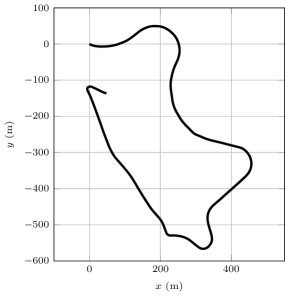
Figure 6: Reference trajectory used during the simulation experiments. It corresponds to a $1.7\text{\,}\mathrm{k}\mathrm{m}$ car trajectory of the KITTI dataset [52] whose duration is $166\text{\,}\mathrm{s}$.

V-C Numerical Example without Biases

To quantitatively assess our preintegration technique against state-of-the-art based on closed-form integration scheme [44] and uncertainty representation [6], we run a numerical experiment where the IMU follows the car trajectory of Figure 6. We gather the path of the sequence 9 of the KITTI dataset [52], from which we differentiate ground-truth and infer true inertial measurements at $\Delta t=$0.1\text{\,}\mathrm{s}$$. The ground-truth is then recomputed with model (22)-(24) to remove integration errors that occur when assuming constant measurements in (29)-(31). We then add Gaussian noise whose covariance is defined as

$$\operatorname{cov}(\boldsymbol{\eta}^{\boldsymbol{\omega}}_{i}) =\alpha\sigma_{\boldsymbol{\omega}}^{2}\mathbf{I}_{3},~{}~{}~{}\operatorname{cov}(\boldsymbol{\eta}^{\mathbf{a}}_{i})=\alpha\sigma_{\mathbf{a}}^{2}\mathbf{I}_{3},$$

where $\sigma_{\boldsymbol{\omega}}$ and $\sigma_{\mathbf{a}}$ are the same as in simulations of [6], i.e. and , and with $\alpha$ a scaling parameter for testing purposes.

The factor covariance is computed using four methods:

1. $SE_{2}(3)$, which computes the covariance based on (66) with accuracy up to second-order;

2. $SO(3)\times\mathbb{R}^{6}$ [6, 44], same as the method 1) but adapted to uncertainty on $SO(3)\times\mathbb{R}^{6}$, i.e. with uncertainty representation of [6] and integration scheme of [44];

3. $SE(3)\times\mathbb{R}^{3}$, same as the method 1) but adapted to uncertainty on $SE(3)\times\mathbb{R}^{3}$ (this method has not appeared before to our knowledge);

4. $SE_{2}(3)$ (Monte-Carlo), which is a slow yet accurate approach. At each time step, we draw a large number $M=${10}^{6}$$ of random samples $\boldsymbol{\xi}^{m}_{ij}$ and $\boldsymbol{\eta}_{j}^{m}$, propagate the resulting states, and compute the covariance as $\boldsymbol{\Sigma}_{i(j+1)}=\frac{1}{M-1}\sum_{m=1}^{M}\boldsymbol{\xi}^{m}\boldsymbol{\xi}^{mT}$ with

   $$\mathbf{T}^{m}=\boldsymbol{\Gamma}_{j}\Phi\left(\mathbf{\hat{T}}_{ij}\exp(\boldsymbol{\xi}^{m}_{ij})\right)\hat{\boldsymbol{\Upsilon}}_{j}\exp(\boldsymbol{\eta}^{m}_{j}),$$

   and $\boldsymbol{\xi}^{m}=\log(\mathbf{\hat{T}}_{i(j+1)}^{-1}\mathbf{T}^{m})$. It requires, e.g., $50M=$5\text{⋅}{10}^{7}$$ samples for one preintegration factor of length $\Delta t_{ij}=$5\text{\,}\mathrm{s}$$. It indicates the best recursive distribution based on $SE_{2}(3)$ one may obtain.

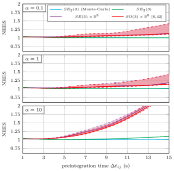
Figure 7: IMU preintegration experiment. NEES criterion based on Monte-Carlo simulations for low noise (above), medium noise (middle), and high noise (bottom). Target value is one, solid curves are the median value, and dashed curves are the 33% and 67% percentiles of the errors. Solid and dashed curves coincide for the $SE_{2}(3)$ methods. The improved performances of the $SE_{2}(3)$ methods are highlighted as the preintegration time gradually scales up.

To evidence the fact that our approach is more consistent, we compute the average Normalized Estimation Error Squared (NEES) as

$$\text{NEES}=\frac{1}{9N}\sum_{n=1}^{N}\mathbf{e}_{n}^{T}\boldsymbol{\Sigma}^{-1}\mathbf{e}_{n},$$

where the error is defined as

$$\mathbf{e}_{n}^{SE_{2}(3)}=\log\big{(}\mathbf{\hat{T}}_{ij}^{-1}\mathbf{\hat{T}}_{ij}^{n}\big{)},\text{~{}~{}or~{}~{}}\mathbf{e}_{n}^{SO(3)\times\mathbb{R}^{6}}=\mathbf{T}_{ij}^{n}\boxminus\mathbf{\hat{T}}_{ij}.$$

We sample $N=${10}^{6}$$ Monte-Carlo noisy preintegrations $\mathbf{T}^{n}_{ij}$ for each factor $\mathbf{T}_{ij}$, where for each Monte-Carlo realization $n$, we compute one realization of each noise $\boldsymbol{\eta}_{i}$, …, $\boldsymbol{\eta}_{j-1}$. If the NEES is higher than 1, the approach is overconfident, if it stays below 1, it is conservative. One usually wants to avoid overconfident estimates.

Results are displayed in Figure 7 for three noise scale parameters and increasing values of the preintegration time. We observe that:

1. $SE_{2}(3)$ distribution is the most consistent approach. This becomes visible as the preintegration time increases for each level of IMU noises;

2. $SO(3)\times\mathbb{R}^{6}$ distribution poorly approximates long preintegration uncertainty, where the median value is close to the 33% percentile while the 67% percentile is much larger. It indicates that there exists some types of trajectory (that correspond to high rotation motions) where the performances of the $SO(3)\times\mathbb{R}^{6}$ on manifold method might degrade. This confirms the results of Section IV-C where we see the average error should be not zero and that linearization errors do occur;

3. $SE(3)\times\mathbb{R}^{3}$ obtains similar results as $SO(3)\times\mathbb{R}^{6}$, and we see that despite the use of $SE(3)$ which is known to describe well uncertainty associated with poses, the full $SE_{2}(3)$ structure is desirable in the context of IMUs;

4. all methods degrade as noise and preintegration time increase because the preintegrated measurements become non-Gaussian. Interestingly, the linearization errors of our $SE_{2}(3)$-based scheme (as opposed to Monte-Carlo estimate) are only visible for high noise ($\alpha=10$) and sufficiently high preintegration time.

V-D Bias Correction via Lie Exponential First-Order Updates

This subsection shows the impact of computing first-order bias corrections using the representation of errors based on exponential coordinates of $SE_{2}(3)$. In the context of preintegration, given a bias update $\hat{\mathbf{b}}^{+}_{i}\leftarrow\hat{\mathbf{b}}_{i}+\delta\mathbf{b}$, one needs to compute how the preintegrated quantities $\hat{\boldsymbol{\Upsilon}}_{ij}$ change. Assume we have computed $\hat{\boldsymbol{\Upsilon}}_{ij}(\hat{\mathbf{b}}_{i})$ corresponding to bias $\hat{\mathbf{b}}_{i}$ and let $\hat{\boldsymbol{\Upsilon}}_{ij}(\hat{\mathbf{b}}_{i}^{+})$ denote the measurement associated to new bias estimation. We define the first-order update as

$$\hat{\boldsymbol{\Upsilon}}_{ij}(\hat{\mathbf{b}}_{i}^{+})=\hat{\boldsymbol{\Upsilon}}_{ij}(\hat{\mathbf{b}}_{i})\exp\Big{(}\frac{\partial\hat{\boldsymbol{\Upsilon}}_{ij}}{\partial\mathbf{b}}|_{\hat{\mathbf{b}}_{i}}\delta\mathbf{b}+O(\|\delta\mathbf{b}\|^{2})\Big{)}.$$ (67)

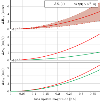
Figure 8: Error committed when using the first-order approximation instead of repeating the integration, for different magnitude of bias updates. Solid curves are the median value, and dashed curves are the 33% and 67% percentiles of the errors. Both methods coincide for the rotation error as they use the same update rule. Solid and dashed curves coincide for the velocity and position errors. Our approach better approximates velocity and position preintegration updates. Statistics are computed over ${10}^{6}$ Monte-Carlo runs for each of the 166 preintegration factors.

The derivation of the Jacobian is similar to the one we use to express the measurements as a large value plus a small perturbation. We first define the variation for one time step

$$\boldsymbol{\Upsilon}_{i}(\hat{\mathbf{b}}_{i}^{+}) =\boldsymbol{\Upsilon}_{i}(\hat{\mathbf{b}}_{i}+\delta\mathbf{b})$$

$$=\hat{\boldsymbol{\Upsilon}}_{i}(\hat{\mathbf{b}}_{i})\exp\big{(}\mathbf{G}_{i}\delta\mathbf{b}+O(\|\delta\mathbf{b}\|^{2})\big{)}$$ (68)

as similarly done in Section III-C, where $\mathbf{G}_{i}$ is defined in (39). We then compute

$$\boldsymbol{\Upsilon}_{ij}(\hat{\mathbf{b}}_{i}^{+}) \stackrel{{\scriptstyle\eqref{eq:ups_batch}}}{{=}}\prod_{k=i}^{j-1}\Phi_{k(j-1)}\left(\hat{\boldsymbol{\Upsilon}}_{k}(\hat{\mathbf{b}}_{i})\exp\left(\mathbf{G}_{k}\delta\mathbf{b}\right)\right)$$

$$\stackrel{{\scriptstyle\eqref{eq:adjoint2}}}{{=}}\hat{\boldsymbol{\Upsilon}}_{ij}(\hat{\mathbf{b}}_{i})\prod_{k=i}^{j-1}\exp\left(\mathbf{A}_{k+1}^{j-1}\mathbf{G}_{k}\delta\mathbf{b}\right)$$

$$\stackrel{{\scriptstyle\eqref{eq:bch2}}}{{=}}\hat{\boldsymbol{\Upsilon}}_{ij}(\hat{\mathbf{b}}_{i})\exp\Big{(}\sum_{k=i}^{j-1}\mathbf{A}_{k+1}^{j-1}\mathbf{G}_{k}\delta\mathbf{b}+O(\|\delta\mathbf{b}\|^{2})\Big{)}.$$ (69)

As in (66), we resort to (48) to compute the Jacobian recursively as

$$\frac{\partial\hat{\boldsymbol{\Upsilon}}_{i(j+1)}}{\partial\mathbf{b}}|_{\hat{\mathbf{b}}_{i}}=\operatorname{Ad}_{\hat{\boldsymbol{\Upsilon}}_{j}}\mathbf{F}\frac{\partial\hat{\boldsymbol{\Upsilon}}_{ij}}{\partial\mathbf{b}}|_{\hat{\mathbf{b}}_{i}}+\mathbf{G}_{j},$$ (70)

starting from initial condition $\frac{\partial\hat{\boldsymbol{\Upsilon}}_{ii}}{\partial\mathbf{b}}|_{\hat{\mathbf{b}}_{i}}=\mathbf{0}_{9\times 6}$.

V-E Numerical Example with Biases

This section shows our matrix formalism and the use of exponential coordinates yield slightly more accurate first-order bias correction than in the theory of [6] (with integration scheme of [44]). The accuracy of this first-order bias correction is reported in Figure 8. To compute the statistics, we integrated the noise-free IMU measurements of Section V-C with a given bias estimate $\hat{\mathbf{b}}_{i}=\mathbf{0}_{3}$ during $\Delta t_{ij}=$1\text{\,}\mathrm{s}$$, which results in the preintegrated measurements $\Delta\mathbf{R}_{ij}(\hat{\mathbf{b}}_{i})$, $\Delta\mathbf{v}_{ij}(\hat{\mathbf{b}}_{i})$ and $\Delta\mathbf{p}_{ij}(\hat{\mathbf{b}}_{i})$. Subsequently, a random perturbation $\delta\mathbf{b}$ with fixed magnitude was applied to both the gyroscope and accelerometer bias (the magnitude of accelerometer bias is 30 times higher than the gyro one). We repeat the integration at $\hat{\mathbf{b}}_{i}+\delta\mathbf{b}$ to obtain $\Delta\mathbf{R}_{ij}(\hat{\mathbf{b}}_{i}+\delta\mathbf{b})$, $\Delta\mathbf{v}_{ij}(\hat{\mathbf{b}}_{i}+\delta\mathbf{b})$ and $\Delta\mathbf{p}_{ij}(\hat{\mathbf{b}}_{i}+\delta\mathbf{b})$. This ground-truth result was then compared against the first-order correction to compute the error of the approximation based on $N=${10}^{6}$$ random perturbation $\delta\mathbf{b}$ for each preintegration factor. The errors resulting from the first-order approximation are small, even for the relatively large bias perturbations, and we see our approach coincides with [6, 44] regarding orientation but obtains more accurate velocity and position preintegration factors.

VI IMU Preintegration on Rotating Earth

This section provides exact closed-form expressions for computing the right-hand side of the factors (58)-(60) when taking into account the Earth rotation, Coriolis acceleration, and centrifugal acceleration. We obtain results that are independent of the uncertainty representation and as such may be used in previous preintegration formalisms [6, 44]. This allows applying factor-graph based optimization techniques to military and civilian applications that require localization over long time scales based on accurate inertial sensors.

VI-A IMU Equations with Rotating Earth

Accounting for Earth rotation, (22)-(24) become [49]

$$\dot{\mathbf{R}} =-\boldsymbol{\Omega}_{\times}\mathbf{R}+\mathbf{R}(\boldsymbol{\omega}^{m}-\mathbf{b}^{\boldsymbol{\omega}}-\boldsymbol{\eta}^{\boldsymbol{\omega}})_{\times},$$ (71)

$$\dot{\mathbf{v}} =\mathbf{R}(\mathbf{a}^{m}-\mathbf{b}^{\mathbf{a}}-\boldsymbol{\eta}^{\mathbf{a}})+\mathbf{g}-2\boldsymbol{\Omega}_{\times}\mathbf{v}-\boldsymbol{\Omega}_{\times}^{2}\mathbf{p},$$ (72)

$$\dot{\mathbf{p}} =\mathbf{v},$$ (73)

where the Earth rotation vector

$$\boldsymbol{\Omega}=\underbrace{\text{Earth rate}}_{\simeq 7.292\times 10^{-5}\text{rad/s}}\times\begin{bmatrix}\cos(\text{latitude})\\ 0\\ -\sin(\text{latitude})\end{bmatrix}\in\mathbb{R}^{3}$$ (74)

is written in the local, i.e. geographic (north, east, down), reference frame, where the Earth rate is approximately $15\text{\,}\mathrm{d}\mathrm{e}\mathrm{g}\mathrm{/}\mathrm{h}$. The term $-2\boldsymbol{\Omega}_{\times}\mathbf{v}$ is called Coriolis acceleration while the term $-\boldsymbol{\Omega}_{\times}^{2}\mathbf{p}$ is called centrifugal acceleration. To be perfectly accurate, this second term is the varying part of the centrifugal acceleration, which actually writes $-\boldsymbol{\Omega}_{\times}^{2}(\mathbf{p}-\mathbf{p}_{0})$ with $\mathbf{p}_{0}$ a point of the Earth rotation axis. But expanding the parenthesis we obtain a constant term $\boldsymbol{\Omega}_{\times}^{2}\mathbf{p}_{0}$ which can be simply added to $\mathbf{g}$. And this is already the case: the $\mathbf{g}$ of approximate value $9.81\text{\,}\mathrm{m}\mathrm{/}\mathrm{s}^{2}$ we are familiar with is actually the sum of the Newton gravitation force and the centrifugal acceleration due to Earth rotation. Hence the residual term $-\boldsymbol{\Omega}_{\times}^{2}\mathbf{p}$.

Remark 8.

In the model (71)-(74) and in the experiments of Section VII, we consider navigation in a local North-East-Down (NED) frame, where we assume the gravity $\mathbf{g}$ and Earth rate $\boldsymbol{\Omega}$ are fixed at their initial values. Although it simplifies the exposition, and is a valid assumption for trajectories that span a dozen of kilometers as in the following experiments, it is by no means a required assumption in our theory. Indeed, the only required assumption is that $\mathbf{g}$, $\boldsymbol{\Omega}$ be fixed during the computation of each factor (which is painless as the latitude virtually does not change during one preintegration): at the beginning of each preintegration $\mathbf{g}$, $\boldsymbol{\Omega}$ may be updated based on the estimated position. In this regard, the algorithm needs to know at least its initial latitude. There is however no way around this assumption, which applies to all algorithms which perform highly precise inertial navigation.

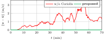
Figure 9: Error committed in term of velocity when neglecting rotating Earth and Coriolis accelerations (red), for a preintegration time interval $\Delta t_{ij}=$5\text{\,}\mathrm{s}$$. IMU measurements are bias- and noise-free, in simulation. The proposed preintegration approach (green) based on (79)-(81) is exact.

VI-B Revisiting IMU Equations with Rotating Earth

Model (71)-(73) does seemingly not lend itself to application of the form (25). However, let us introduce the variable

$$\mathbf{T}^{\prime}:=\begin{bmatrix}\begin{array}[]{c|c|c}\mathbf{R}&\mathbf{v}+\boldsymbol{\Omega}_{\times}\mathbf{p}&\mathbf{p}\\ \hline\cr\mathbf{0}_{2\times 3}&\lx@intercol\hfil\mathbf{I}_{2}\hfil\lx@intercol\end{array}\end{bmatrix}.$$ (75)

This trick allows embedding the auxiliary state $\mathbf{T}^{\prime}_{t}$ into the form of (25) as

$$\mathbf{T}_{t}^{\prime}=\boldsymbol{\Gamma}_{t}^{\prime}\Phi_{t}(\mathbf{T}_{0}^{\prime})\boldsymbol{\Upsilon}_{t},$$ (76)

where $\boldsymbol{\Upsilon}_{t}$ is the same as in (25) and $\boldsymbol{\Gamma}^{\prime}_{t}$ is obtained after solving the differential equations

$$\dot{\boldsymbol{\Gamma}}_{t}^{\prime}:=\begin{bmatrix}\begin{array}[]{c|cc}\dot{\boldsymbol{\Gamma}}^{\mathbf{R}}&\dot{\boldsymbol{\Gamma}}^{\mathbf{v}}&\dot{\boldsymbol{\Gamma}}^{\mathbf{p}}\\ \hline\cr\mathbf{0}_{2\times 3}&\lx@intercol\hfil\mathbf{I}_{2}\hfil\lx@intercol\end{array}\end{bmatrix},$$ (77)

where

$$\dot{\boldsymbol{\Gamma}}^{\mathbf{R}}=-\boldsymbol{\Omega}_{\times}\boldsymbol{\Gamma}^{\mathbf{R}},~{}~{}\dot{\boldsymbol{\Gamma}}^{\mathbf{v}}=\mathbf{g}-\boldsymbol{\Omega}_{\times}\boldsymbol{\Gamma}^{\mathbf{v}},~{}~{}\dot{\boldsymbol{\Gamma}}^{\mathbf{p}}=\boldsymbol{\Gamma}^{\mathbf{v}}-\boldsymbol{\Omega}_{\times}\boldsymbol{\Gamma}^{\mathbf{p}},$$

initialized at $\boldsymbol{\Gamma}^{\mathbf{R}}=\mathbf{I}_{3}$, $\boldsymbol{\Gamma}^{\mathbf{v}}=\mathbf{0}_{3}$, $\boldsymbol{\Gamma}^{\mathbf{p}}=\mathbf{0}_{3}$, and that do not involve the state, see proofs in [8] and supplementary materials.

We solve for $\mathbf{T}^{\prime}_{t}$ and apply our framework for preintegration as follows. First, we define an exact discrete model

$$\mathbf{T}_{j}^{\prime}=\boldsymbol{\Gamma}_{ij}^{\prime}\Phi_{ij}(\mathbf{T}_{i}^{\prime})\boldsymbol{\Upsilon}_{ij},$$ (78)

between instants $t_{i}$ and $t_{j}$, as performed in Section IV-D, that leads to

$$\mathbf{R}_{j} =\boldsymbol{\Gamma}^{\mathbf{R}}_{ij}\mathbf{R}_{i}\Delta\mathbf{R}_{ij},$$ (79)

$$\mathbf{v}_{j} =\boldsymbol{\Gamma}^{\mathbf{v}}_{ij}+\boldsymbol{\Gamma}^{\mathbf{R}}_{ij}\left(\mathbf{R}_{i}\Delta\mathbf{v}_{ij}+\mathbf{v}_{i}+\boldsymbol{\Omega}_{\times}\mathbf{p}_{i}\right)-\boldsymbol{\Omega}_{\times}\mathbf{p}_{j},$$ (80)

$$\mathbf{p}_{j} =\boldsymbol{\Gamma}^{\mathbf{p}}_{ij}+\boldsymbol{\Gamma}^{\mathbf{R}}_{ij}\left(\mathbf{R}_{i}\Delta\mathbf{p}_{ij}+\left(\mathbf{v}_{i}+\boldsymbol{\Omega}_{\times}\mathbf{p}_{i}\right)\Delta t_{ij}+\mathbf{p}_{i}\right),$$ (81)

where $\Delta\mathbf{R}_{ij}$, $\Delta\mathbf{v}_{ij}$, $\Delta\mathbf{p}_{ij}$ are yet given through (29)-(31) while $\boldsymbol{\Gamma}^{\mathbf{R}}_{ij}$, $\boldsymbol{\Gamma}^{\mathbf{v}}_{ij}$, $\boldsymbol{\Gamma}^{\mathbf{p}}_{ij}$ are defined as

$$\boldsymbol{\Gamma}^{\mathbf{R}}_{ij} =\exp(-\Delta t_{ij}\boldsymbol{\Omega}),$$ (82)

$$\boldsymbol{\Gamma}^{\mathbf{v}}_{ij} =\mathbf{\mathcal{J}}_{-\Delta t_{ij}\boldsymbol{\Omega}}\Delta t_{ij}\mathbf{g},$$ (83)

$$\boldsymbol{\Gamma}^{\mathbf{p}}_{ij} =\big{(}\frac{\Delta t^{2}}{2}\mathbf{I}_{3}+a\boldsymbol{\Omega}_{\times}+b\boldsymbol{\Omega}_{\times}^{2}\big{)}\mathbf{g},$$ (84)

with $\phi=\|\boldsymbol{\Omega}\|$, $a=\phi^{-3}(\phi\Delta t_{ij}\cos(\phi\Delta t_{ij})-\sin(\phi\Delta t_{ij}))$, and $b=\phi^{-4}(\frac{\phi^{2}\Delta t_{ij}^{2}}{2}-\cos(\phi\Delta t_{ij})-\phi\Delta t_{ij}\sin(\Delta t_{ij}\phi)+1)$. To express preintegration factors as function of states, we compute

$$\boldsymbol{\Upsilon}_{ij} \stackrel{{\scriptstyle\eqref{eq:tij}}}{{=}}\Big{(}\boldsymbol{\Gamma}^{\prime}_{ij}\Phi_{ij}\left(\mathbf{T}^{\prime}_{i}\right)\Big{)}^{-1}\mathbf{T}^{\prime}_{j},$$ (85)

see the similarity with (61), that we finally develop as

$$\Delta\mathbf{R}_{ij} \stackrel{{\scriptstyle\eqref{eq:Rcoriolis}}}{{=}}\big{(}\boldsymbol{\Gamma}^{\mathbf{R}}_{ij}\mathbf{R}_{i}\big{)}^{T}\mathbf{R}_{j},$$ (86)

$$\Delta\mathbf{v}_{ij} \stackrel{{\scriptstyle\eqref{eq:vcoriolis}}}{{=}}\mathbf{R}_{i}^{T}\big{(}\boldsymbol{\Gamma}^{\mathbf{R}T}_{ij}\left(\mathbf{v}_{j}+\boldsymbol{\Omega}_{\times}\mathbf{p}_{j}-\boldsymbol{\Gamma}_{ij}^{\mathbf{v}}\right)-\mathbf{v}_{i}-\boldsymbol{\Omega}_{\times}\mathbf{p}_{i}\big{)},$$ (87)

$$\Delta\mathbf{p}_{ij} \stackrel{{\scriptstyle\eqref{eq:pcoriolis}}}{{=}}\mathbf{R}_{i}^{T}\big{(}\boldsymbol{\Gamma}^{\mathbf{R}T}_{ij}\left(\mathbf{p}_{j}-\boldsymbol{\Gamma}^{\mathbf{p}}_{ij}\right)-\left(\mathbf{v}_{i}+\boldsymbol{\Omega}_{\times}\mathbf{p}_{i}\right)\Delta t_{ij}-\mathbf{p}_{i}\big{)}.$$ (88)

To summarize, preintegrating IMU with rotating Earth consists in substituting (58)-(60) by (86)-(88), and leaving the covariance noise computation unchanged, as Coriolis and centrifugal accelerations leave the left-hand side of the preintegrated factors unchanged, and thus the quantity $\boldsymbol{\Upsilon}_{ij}$ in (85) is yet defined in (64). These results are obtained independently from a choice for uncertainty representation, and as such they may also be used in current implementations such as [6].

We confirm our results with a numerical example, see Figure 9, where we preintegrate bias- and noise-free IMU measurements for a long car trajectory. Similarly as in Section V-C, we differentiate the ground-truth trajectory of the sequence 1 of our real experiments (see Section VII) to obtain true inertial measurements. Then the ground-truth is recomputed with model (71)-(73) to remove integration errors. We compute the error when neglecting the rotation of the Earth ($\boldsymbol{\Omega}=\mathbf{0}_{3}$) versus our approach with $\Delta t_{ij}=$5\text{\,}\mathrm{s}$$. We see no error at the beginning of the sequence as the car is static. Then the error committed when neglecting the rotating Earth grows, whereas our approach is exact.

Remark 9.

[53, 27] attack factor-graph based accurate navigation, and provide the following formulas for preintegration with Coriolis acceleration in the appendix of [53]

$$v_{j}^{L_{j}}=R^{L^{j}}_{L_{i}}\Big{(}v_{i}^{L_{i}}+R^{L_{i}}_{b_{i}}\Delta v^{b_{i}}_{i\rightarrow j}+[g^{L_{i}}-\frac{(w_{iL_{i}}^{L_{i}})_{\times}v_{j}^{L_{j}}}{2}]\Delta t_{ij}\Big{)}.$$

The authors obtain a term $-2(\omega_{i^{L}_{i}})_{\times}v_{i}^{L_{i}}$ in place of the expected $-2(\omega_{i^{L}_{i}})_{\times}v_{j}^{L_{j}}$ (index $i$ of $v$ should be $j$): we see the Coriolis term of [53] is actually approximated by its value at initial time $t_{i}$.

IMU noise parameters	ours	simu. of [6]
gyro rand. walk, rad/(sHz)	$9.4\text{⋅}{10}^{-6}$	$7\text{⋅}{10}^{-4}$
acc. rand. walk, m/(s^2Hz)	$4.2\text{⋅}{10}^{-3}$	$1.9\text{⋅}{10}^{-2}$
gyro bias rand. walk, rad/(s^2Hz)	$1.6\text{⋅}{10}^{-6}$	$4\text{⋅}{10}^{-4}$
acc. bias rand. walk, m/(s^3Hz)	$5.4\text{⋅}{10}^{-5}$	$1.2\text{⋅}{10}^{-2}$

Table 1: Values of the IMU noise parameters used in our algorithms during real experiments, compared to the ones of [6].

seq.	length	dur.	LiDAR		LiDAR-IMU w/o Coriolis		LiDAR-IMU w Coriolis (proposed)
	km	min	rot. err. ($\mathrm{d}\mathrm{e}\mathrm{g}\mathrm{/}\mathrm{k}\mathrm{m}$)	trans. err. ($\mathrm{m}\mathrm{/}\mathrm{k}\mathrm{m}$)	rot. err. ($\mathrm{d}\mathrm{e}\mathrm{g}\mathrm{/}\mathrm{k}\mathrm{m}$)	trans. err. ($\mathrm{m}\mathrm{/}\mathrm{k}\mathrm{m}$)	rot. err. ($\mathrm{d}\mathrm{e}\mathrm{g}\mathrm{/}\mathrm{k}\mathrm{m}$)	trans. err. ($\mathrm{m}\mathrm{/}\mathrm{k}\mathrm{m}$)
1	27	73	1.6   /   0.9	15   /   19	1.3   /   0.6	15   /    8	0.9   /   0.3	15   /    6
2	37	101	1.5   /   0.9	14   /   12	0.9   /   0.6	13   /   10	0.6   /   0.3	13   /    7
3	3	7	3.0   /   1.7	16   /    9	1.5   /   0.2	14   /    4	1.4   /   0.3	15   /    4
4	8	19	1.7   /   1.1	19   /   22	0.8   /   0.3	18   /   11	1.1   /   0.3	17   /    6
5	4	11	2.7   /   1.6	16   /    9	1.0   /   0.4	16   /    5	1.0   /   0.5	16   /    5
6	74	73	3.9   /   0.9	37   /   26	2.6   /   0.4	38   /   25	2.6   /   0.4	35   /   24
total	153	284	2.6   /   0.9	25   /   19	1.7   /   0.5	25   /   16	1.6   /   0.3	23   /   14

Table 2: Real experiment results in terms of relative translation (trans. err.) and relative rotational (rot. err.) errors based on short (left) and long (right) sub-sequences. Taking into account IMU during estimation improves each metric. Considering rotating Earth and Coriolis acceleration is more beneficial for long-term navigation.

VII Real Experiments

This section addresses sensor-fusion of a high-grade IMU with relative translations provided by a LiDAR in a fixed-lag smoother for long-term navigation. Building on the preintegration with rotating Earth and Coriolis effect formulas developed in Section VI, we implement our loosely-coupled approach with the GTSAM factor-graph library [24].

We gathered more than 150 km and four hours of data divided into six sequences. The vehicle acquires data around the R&T centre of SafranTech located at Magny-Les-Hameaux, France. The car embeds a high-grade IMU manufactured by Safran Electronics and Defense, whose increments are acquired at $100\text{\,}\mathrm{H}\mathrm{z}$, and a Velodyne LiDAR VLP32C which is mounted on top of the car. Table 1 indicates the IMU noise specifications that we set in our algorithms and which are two orders of magnitude lower than those used in the simulations of [6]. The 3D laser scans between keyframes are preprocessed to obtain relative transformations using scan matching algorithms. The vehicle is finally equipped with a RTK-GPS antenna which outputs positions and yaws that we consider as ground-truth. This dataset is challenging regarding the length of the sequences, the car velocity (up to $30\text{\,}\mathrm{m}\mathrm{/}\mathrm{s}$), and the presence of many bumps, sharp curves and roundabouts on the way.

VII-A Compared Methods & Algorithm Setting

Owing the precision of the gyroscopes, relative orientation between LiDAR’s point clouds does not bring additional relevant information, and we focus only on the relative translations returned by the LiDAR. We compare three approaches for estimating the vehicle pose using the IMU and the LiDAR:

1. LiDAR, which is the compound of the relative poses estimated by the scan matching algorithms as in (1);

2. LiDAR-IMU w/o Coriolis, which is the fusion between the relative translations given by the scan matching algorithms and the inertial signals, without considering rotating Earth and Coriolis force, i.e. assuming $\boldsymbol{\Omega}=\mathbf{0}_{3}$;

3. LiDAR-IMU w Coriolis, same as method 2), but where rotating Earth and Coriolis force are considered and $\boldsymbol{\Omega}$ defined with the latitude at which each sequence starts ($48.73\text{\,}\mathrm{d}\mathrm{e}\mathrm{g}$).

The LiDAR-aided approaches are described as follows. We implement a fixed-lag smoother based on iSAM2 [9] from the GTSAM library [24]. Our GTSAM fork computes the bias update correction with Lie exponential coordinates (67), preintegrates with rotating Earth and Coriolis force (79)-(81), and leaves the retraction of the extended pose (a.k.a. navigation state in [24]) unchanged. Biases are estimated along with extended poses through CombinedImuFactor, and initialized with the beginning of each sequence, where the car is static. Each approach performs odometry estimation, i.e., it estimates the car trajectory relative to its starting position without using global information from GNSS or LiDAR loop-closure.

Scan matching algorithms return relative orientation and translation, where the level of rotation uncertainty between LiDAR scans is much higher than the gyro’s uncertainty (assuming the gyro bias is known, the gyro only drifts of less than a few degrees in one hour, which is lower than the Earth rotation rate). Therefore, we fed the factor-graph with IMU preintegrated factors, relative translation factors, and zero upward velocity factor with a relatively small standard deviation of $1\text{\,}\mathrm{m}\mathrm{/}\mathrm{s}$ to prevent the upward velocity from drifting, as used, e.g., in [54].

We set the smoother with a lag of $20\text{\,}\mathrm{s}$, insert each factor at $4\text{\,}\mathrm{H}\mathrm{z}$, and define its noise parameters as follows. Then the covariance of the discrete-time noise $\boldsymbol{\eta}^{\mathrm{d}}$ is computed as a function of the sampling rate and relates to the continuous-time spectral noise $\boldsymbol{\eta}^{\mathrm{c}}$ via $\operatorname{cov}(\boldsymbol{\eta}^{\mathrm{d}})=\operatorname{cov}(\boldsymbol{\eta}^{\mathrm{c}})/\Delta t$ [55]. Relative translations are given with an uncertainty of $20\text{\,}\mathrm{c}\mathrm{m}$ in each direction, and we make the translation factor more robust during high motions with a Huber loss. Finally, the initial orientation and position are provided from the ground-truth, and the initial velocity is null.

VII-B Evaluation Metrics

To assess performances we recall the error metrics proposed in the KITTI dataset [52]:

• Relative translation error, which is computed as

  $$\text{trans. err.}=\left\|\mathbf{R}_{i}^{T}(\mathbf{p}_{j}-\mathbf{p}_{i})-\hat{\mathbf{R}}_{i}^{T}(\hat{\mathbf{p}}_{j}-\hat{\mathbf{p}}_{i})\right\|_{2}$$

  after an alignment transformation for all sub-sequences of length $100\text{\,}\mathrm{m}$, …, $800\text{\,}\mathrm{m}$;

• Relative rotational error, which is computed as

  $$\text{rot. err.}=\left\|\log\big{(}(\mathbf{R}_{i}^{T}\mathbf{R}_{j})^{T}(\hat{\mathbf{R}}_{i}^{T}\hat{\mathbf{R}}_{j})\big{)}\right\|_{2}$$

  for all sub-sequences of length $100\text{\,}\mathrm{m}$, …, $800\text{\,}\mathrm{m}$.

As advocated in [56], these metrics are recommended for comparing odometry estimation methods since they are barely sensitive to the time when the estimation error occurs. We adapt theses metrics as follows: the approaches are evaluated in the horizontal plan as the ground-truth is as accurate as the estimation algorithms to compute the pitch and the roll, and we compute both short- and long-term metrics. In total, we compute three sets of pairs {rot. err., trans. err.}:

1. a set of short-term errors based on sub-sequences of length $100\text{\,}\mathrm{m}$, …, $800\text{\,}\mathrm{m}$ as in [52];

2. a set of long-term errors based on sub-sequences of length $1\text{\,}\mathrm{k}\mathrm{m}$, …, $8\text{\,}\mathrm{k}\mathrm{m}$, as rotating Earth and Coriolis effect are more visible after long traveled distances;

3. a set of errors for sub-sequences of duration $3\text{\,}\mathrm{m}\mathrm{i}\mathrm{n}$, …, $15\text{\,}\mathrm{m}\mathrm{i}\mathrm{n}$. Indeed, the error of odometry methods based on LiDAR or vision should grow with distance whereas that methods based on IMU should grow with time.

VII-C Result Analysis & Discussion

Table 2 provides numerical results for the two first sets of evaluation metrics, and Figure 11 displays results for the third set. We observe:

1. the LiDAR estimates highly efficiently the distances and stays accurate in straight lines. However, it has difficulties in areas with tight curves, roundabouts (where visual ambiguity might play a role), or when the car is moving fast;

2. as the LiDAR loses accuracy in decisive but rare moments such as roundabouts, the short-term results of Table 2 are correct, and one mainly tries to improve the long-term metrics;

3. only relative translation information is sufficient to obtain a robust loosely-coupled estimation from the IMU and the LiDAR. This solves most of the problems encountered by the LiDAR during sharp curves and roundabouts;

4. the two LiDAR inertial approaches have similar results for the shortest sequences 3 and 5, see Table 2. Indeed, for a small sequence, Coriolis force is negligible and the Earth rotation rate may be inserted in bias;

5. taking into account Coriolis increases accuracy for long distances, see the long-term metrics in Table 2, where the one that considers Coriolis is about one hundred meter away from the ground after more than one hour of odometry, without GNSS or LiDAR loop-closure;

6. Figure 11 shows approximately linear grow of the error with respect to time. Considering rotating Earth and Coriolis effect improves the translation metric from $130\text{\,}\mathrm{m}$ to $103\text{\,}\mathrm{m}$, i.e. an improvement of 21%, with sub-sequences of length $15\text{\,}\mathrm{m}\mathrm{i}\mathrm{n}$.

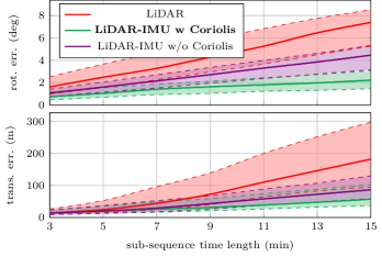
Fig. 11: Real experiment results in terms of relative rotation (rot. err.) and relative translation (trans. err.) errors based on sub-sequences of duration 3, …, 15 minutes. Solid curves are the median value, and dashed curves are the 33% and 67% percentiles of the errors. Considering rotating Earth and Coriolis force appears beneficial for orientation and translation from sub-sequences of length 7 minutes.

These results show how beneficial it is to consider rotating Earth and Coriolis force in IMU preintegration theory. However, our experiments do not show the advantage of the Lie exponential update of the bias. Indeed, the differences between the proposed bias update and the standard one remains below, e.g., parameter tuning. The benefit of bias update with exponential Lie update does not necessary require long sequences but more accurate localization systems and larger preintegration times.

In our experiments, we take into account the rotation of the Earth but not its curvature (otherwise it would be necessary to consider the variations of longitude, latitude, ellipsoidal altitude, and transport rate). This point is justified by the relatively small area covered by the trajectories, and the fact that we are estimating relative trajectories. We anticipate the proposed approach would provide even more improvements for long-term navigation with absolute measurements and long distances, e.g. for a plane, a drone, or autonomous underwater vehicles equipped with accurate inertial sensors.

VIII Conclusion

This paper presents some generic techniques to associate uncertainty to an extended pose (three dimensional orientation, velocity and position of a rigid body) and shows how to propagate associated uncertainties with fourth-order accuracy in noise variables and second order in the associated covariances. The framework additionally provides an elegant mathematical approach that brings further maturity to the theory of preintegration on manifold. It unifies flat and rotating Earth IMU equations within a single framework, hence providing extensions of the theory of preintegration with Coriolis force. The method compares favorably against state-of-the-art in extensive simulations, and has been validated for one hour long car navigation in an efficient fixed-lag smoother that fuses IMU and relative translations provided by a LiDAR.

Looking forward, we believe these techniques open up for novel implementations of factor-graph based methods to the context of long term inertial-aided navigation systems, hence genuine industrial navigation systems. Finally, the theory could find application in other problems requiring detailed bookkeeping of extended pose uncertainties. Indeed, our approach with fine uncertainty representation may prove decisive for finely detecting GNSS outliers with preintegration[51], or when we search to accurately define the uncertainty of distant relative extended poses in an (extended) pose-graph. This is outlined by the example of Section IV-C where our approach improves the mean and the uncertainty of the estimates of existing approaches it is compared to.

-A $SO(3)$ & $SE_{2}(3)$ Closed-Form Expressions

Let $\boldsymbol{\phi}\in\mathbb{R}^{3}$ and $\mathbf{R}\in SO(3)$. The exponential, logarithm, left-Jacobian and inverse left-Jacobian of $SO(3)$ are given as

$$\exp(\boldsymbol{\phi}) =\mathbf{I}_{3}+\frac{\sin\phi}{\phi}\boldsymbol{\phi}_{\times}+\frac{1-\cos\phi}{\phi^{2}}\boldsymbol{\phi}_{\times}^{2},$$ (89)

$$\log(\mathbf{R}) =\frac{\varphi}{2\sin\varphi}(\mathbf{R}-\mathbf{R}^{T})^{\vee},$$ (90)

$$\mathbf{\mathcal{J}}_{\boldsymbol{\phi}} =\mathbf{I}_{3}+\frac{1-\cos\phi}{\phi^{2}}\boldsymbol{\phi}_{\times}+\frac{\phi-\sin\phi}{\phi^{3}}\boldsymbol{\phi}_{\times}^{2},$$ (91)

$$\mathbf{\mathcal{J}}^{-1}_{\boldsymbol{\phi}} =\mathbf{I}_{3}-\frac{1}{2}\boldsymbol{\phi}_{\times}+\left(\phi^{-2}+\frac{1+\cos\phi}{2\phi\sin\phi}\right)\boldsymbol{\phi}_{\times}^{2},$$ (92)

where $\vee$ is the linear inverse operator of $\wedge$, $\phi=\|\boldsymbol{\phi}\|$ and $\varphi=\cos^{-1}(\frac{\operatorname{trace}(\mathbf{R})-1}{2})$. Let $\boldsymbol{\xi}\in\mathbb{R}^{9}$ and $\mathbf{T}\in SE_{2}(3)$. The exponential and logarithm of $SE_{2}(3)$ are computed in overloaded operators as

$$\exp(\boldsymbol{\xi})=\begin{bmatrix}\exp(\boldsymbol{\phi})&\mathbf{\mathcal{J}}_{\boldsymbol{\phi}}\boldsymbol{\nu}&\mathbf{\mathcal{J}}_{\boldsymbol{\phi}}\boldsymbol{\rho}\\ \mathbf{0}_{3}^{T}&1&0\\ \mathbf{0}_{3}^{T}&0&1\end{bmatrix},\hfill\log(\mathbf{T})=\begin{bmatrix}\log(\mathbf{R})\\ \mathbf{\mathcal{J}}^{-1}_{\log(\mathbf{R})}\boldsymbol{\nu}\\ \mathbf{\mathcal{J}}^{-1}_{\log(\mathbf{R})}\boldsymbol{\rho}\end{bmatrix}.$$ (93)

The Jacobian for $SE_{2}(3)$ and its inverse are derived from those for $SE(3)$ introduced in [5] as

$$\mathbf{\mathcal{J}}_{\boldsymbol{\xi}} :=\begin{bmatrix}\mathbf{\mathcal{J}}_{\boldsymbol{\phi}}&\mathbf{0}_{3\times 3}&\mathbf{0}_{3\times 3}\\ \mathcal{Q}_{\boldsymbol{\phi},\boldsymbol{\nu}}&\mathbf{\mathcal{J}}_{\boldsymbol{\phi}}&\mathbf{0}_{3\times 3}\\ \mathcal{Q}_{\boldsymbol{\phi},\boldsymbol{\rho}}&\mathbf{0}_{3\times 3}&\mathbf{\mathcal{J}}_{\boldsymbol{\phi}}\end{bmatrix},$$ (94)

$$\mathbf{\mathcal{J}}^{-1}_{\boldsymbol{\xi}} :=\begin{bmatrix}\mathbf{\mathcal{J}}^{-1}_{\boldsymbol{\phi}}&\mathbf{0}_{3\times 3}&\mathbf{0}_{3\times 3}\\ -\mathbf{\mathcal{J}}^{-1}_{\boldsymbol{\phi}}\mathcal{Q}_{\boldsymbol{\phi},\boldsymbol{\nu}}\mathbf{\mathcal{J}}^{-1}_{\boldsymbol{\phi}}&\mathbf{\mathcal{J}}^{-1}_{\boldsymbol{\phi}}&\mathbf{0}_{3\times 3}\\ -\mathbf{\mathcal{J}}^{-1}_{\boldsymbol{\phi}}\mathcal{Q}_{\boldsymbol{\phi},\boldsymbol{\rho}}\mathbf{\mathcal{J}}^{-1}_{\boldsymbol{\phi}}&\mathbf{0}_{3\times 3}&\mathbf{\mathcal{J}}^{-1}_{\boldsymbol{\phi}}\end{bmatrix},$$ (95)

$$\mathcal{Q} {}_{\boldsymbol{\phi},\boldsymbol{\nu}}:=\frac{1}{2}\boldsymbol{\nu}_{\times}+\frac{\phi-\sin\phi}{\phi^{3}}\left(\boldsymbol{\phi}_{\times}\boldsymbol{\nu}_{\times}+\boldsymbol{\nu}_{\times}\boldsymbol{\phi}_{\times}+\boldsymbol{\phi}_{\times}\boldsymbol{\nu}_{\times}\boldsymbol{\phi}_{\times}\right)$$

$$+\frac{\phi^{2}+2\cos\phi-2}{\phi^{4}}\left(\boldsymbol{\phi}_{\times}\boldsymbol{\phi}_{\times}\boldsymbol{\nu}_{\times}+\boldsymbol{\nu}_{\times}\boldsymbol{\phi}_{\times}\boldsymbol{\phi}_{\times}-3\boldsymbol{\phi}_{\times}\boldsymbol{\nu}_{\times}\boldsymbol{\phi}_{\times}\right)$$

$$+\frac{2\phi-3\sin\phi+\phi\cos\phi}{2\phi^{5}}\left(\boldsymbol{\phi}_{\times}\boldsymbol{\nu}_{\times}\boldsymbol{\phi}_{\times}\boldsymbol{\phi}_{\times}+\boldsymbol{\phi}_{\times}\boldsymbol{\phi}_{\times}\boldsymbol{\nu}_{\times}\boldsymbol{\phi}_{\times}\right),$$ (96)

and $\mathcal{Q}_{\boldsymbol{\phi},\boldsymbol{\rho}}$ is defined similarly as (96), replacing $\boldsymbol{\nu}$ by $\boldsymbol{\rho}$.

-B Third- and Fourth-Order Contributions

We compute the quantity $\mathbf{S}_{\text{4th}}$ in (48) along the lines of [5]. Les us define the operators

$$\ll\mathbf{A}\gg :=-\operatorname{trace}(\mathbf{A})\mathbf{I}_{3}+\mathbf{A},$$ (97)

$$\ll\mathbf{A},\mathbf{B}\gg :=\ll\mathbf{A}\gg\ll\mathbf{B}\gg+\ll\mathbf{B},\mathbf{A}\gg,$$ (98)

and $\boldsymbol{\Sigma}=\mathbf{A}_{i}\boldsymbol{\Sigma}_{i+1}\mathbf{A}_{i}^{T}$. We obtain

$$\mathbf{S}_{\text{4th}}=\frac{1}{12}\left(\mathbf{A}_{\boldsymbol{\Sigma}}\mathbf{Q}+\mathbf{Q}\mathbf{A}_{\boldsymbol{\Sigma}}^{T}+\mathbf{A}_{\mathbf{Q}}\boldsymbol{\Sigma}+\boldsymbol{\Sigma}\mathbf{A}_{\mathbf{Q}}^{T}\right)+\frac{1}{4}\mathbf{B},$$ (99)

where

$$\mathbf{A}_{\boldsymbol{\Sigma}} =\begin{bmatrix}\ll\boldsymbol{\Sigma}_{\boldsymbol{\phi}\boldsymbol{\phi}}\gg&\mathbf{0}_{3\times 3}&\mathbf{0}_{3\times 3}\\ \ll\boldsymbol{\Sigma}_{\boldsymbol{\nu}\boldsymbol{\phi}}+\boldsymbol{\Sigma}_{\boldsymbol{\phi}\boldsymbol{\nu}}\gg&\ll\boldsymbol{\Sigma}_{\boldsymbol{\phi}\boldsymbol{\phi}}\gg&\mathbf{0}_{3\times 3}\\ \ll\boldsymbol{\Sigma}_{\boldsymbol{\rho}\boldsymbol{\phi}}+\boldsymbol{\Sigma}_{\boldsymbol{\phi}\boldsymbol{\rho}}\gg&\mathbf{0}_{3\times 3}&\ll\boldsymbol{\Sigma}_{\boldsymbol{\phi}\boldsymbol{\phi}}\gg,\end{bmatrix},$$

$$\mathbf{A}_{\mathbf{Q}} =\begin{bmatrix}\ll\mathbf{Q}_{\boldsymbol{\phi}\boldsymbol{\phi}}\gg&\mathbf{0}_{3\times 3}&\mathbf{0}_{3\times 3}\\ \ll\mathbf{Q}_{\boldsymbol{\nu}\boldsymbol{\phi}}+\mathbf{Q}_{\boldsymbol{\phi}\boldsymbol{\nu}}\gg&\ll\mathbf{Q}_{\boldsymbol{\phi}\boldsymbol{\phi}}\gg&\mathbf{0}_{3\times 3}\\ \ll\mathbf{Q}_{\boldsymbol{\rho}\boldsymbol{\phi}}+\mathbf{Q}_{\boldsymbol{\phi}\boldsymbol{\rho}}\gg&\mathbf{0}_{3\times 3}&\ll\mathbf{Q}_{\boldsymbol{\phi}\boldsymbol{\phi}}\gg\end{bmatrix},$$

$$\mathbf{B}_{\boldsymbol{\phi}\boldsymbol{\phi}} =\ll\boldsymbol{\Sigma}_{\boldsymbol{\phi}\boldsymbol{\phi}},\mathbf{Q}_{\boldsymbol{\phi}\boldsymbol{\phi}}\gg,$$ (100)

$$\mathbf{B}_{\boldsymbol{\nu}\boldsymbol{\phi}} =\mathbf{B}_{\boldsymbol{\phi}\boldsymbol{\nu}}^{T}=\ll\boldsymbol{\Sigma}_{\boldsymbol{\phi}\boldsymbol{\phi}},\mathbf{Q}_{\boldsymbol{\phi}\boldsymbol{\nu}}\gg+\ll\boldsymbol{\Sigma}_{\boldsymbol{\nu}\boldsymbol{\phi}},\mathbf{Q}_{\boldsymbol{\phi}\boldsymbol{\phi}}\gg,$$ (101)

$$\mathbf{B}_{\boldsymbol{\rho}\boldsymbol{\phi}} =\mathbf{B}_{\boldsymbol{\phi}\boldsymbol{\rho}}^{T}=\ll\boldsymbol{\Sigma}_{\boldsymbol{\phi}\boldsymbol{\phi}},\mathbf{Q}_{\boldsymbol{\phi}\boldsymbol{\rho}}\gg+\ll\boldsymbol{\Sigma}_{\boldsymbol{\rho}\boldsymbol{\phi}},\mathbf{Q}_{\boldsymbol{\phi}\boldsymbol{\phi}}\gg,$$ (102)

$$\mathbf{B}_{\boldsymbol{\nu}\boldsymbol{\nu}} =\ll\boldsymbol{\Sigma}_{\boldsymbol{\phi}\boldsymbol{\phi}},\mathbf{Q}_{\boldsymbol{\nu}\boldsymbol{\nu}}\gg+\ll\boldsymbol{\Sigma}_{\boldsymbol{\phi}\boldsymbol{\nu}},\mathbf{Q}_{\boldsymbol{\nu}\boldsymbol{\phi}}\gg$$

$$+\ll\boldsymbol{\Sigma}_{\boldsymbol{\nu}\boldsymbol{\phi}},\mathbf{Q}_{\boldsymbol{\nu}\boldsymbol{\phi}}\gg+\ll\boldsymbol{\Sigma}_{\boldsymbol{\nu}\boldsymbol{\nu}},\mathbf{Q}_{\boldsymbol{\phi}\boldsymbol{\phi}}\gg,$$ (103)

$$\mathbf{B}_{\boldsymbol{\nu}\boldsymbol{\rho}} =\mathbf{B}_{\boldsymbol{\rho}\boldsymbol{\nu}}^{T}=\ll\boldsymbol{\Sigma}_{\boldsymbol{\nu}\boldsymbol{\rho}},\mathbf{Q}_{\boldsymbol{\phi}\boldsymbol{\phi}}\gg+\ll\boldsymbol{\Sigma}_{\boldsymbol{\phi}\boldsymbol{\rho}},\mathbf{Q}_{\boldsymbol{\nu}\boldsymbol{\phi}}\gg$$

$$+\ll\boldsymbol{\Sigma}_{\boldsymbol{\nu}\boldsymbol{\phi}},\mathbf{Q}_{\boldsymbol{\rho}\boldsymbol{\phi}}\gg+\ll\boldsymbol{\Sigma}_{\boldsymbol{\phi}\boldsymbol{\phi}},\mathbf{Q}_{\boldsymbol{\nu}\boldsymbol{\rho}}\gg,$$ (104)

$$\mathbf{B}_{\boldsymbol{\rho}\boldsymbol{\rho}} =\ll\boldsymbol{\Sigma}_{\boldsymbol{\phi}\boldsymbol{\phi}},\mathbf{Q}_{\boldsymbol{\rho}\boldsymbol{\rho}}\gg+\ll\boldsymbol{\Sigma}_{\boldsymbol{\phi}\boldsymbol{\rho}},\mathbf{Q}_{\boldsymbol{\rho}\boldsymbol{\phi}}\gg$$

$$+\ll\boldsymbol{\Sigma}_{\boldsymbol{\rho}\boldsymbol{\phi}},\mathbf{Q}_{\boldsymbol{\phi}\boldsymbol{\rho}}\gg+\ll\boldsymbol{\Sigma}_{\boldsymbol{\rho}\boldsymbol{\rho}},\mathbf{Q}_{\boldsymbol{\phi}\boldsymbol{\phi}}\gg.$$ (105)

References

- [1] R. Hartley and A. Zisserman, Multiple View Geometry in Computer Vision. Cambridge University Press, 2004.
- [2] T. Barfoot, State Estimation for Robotics. Cambridge University Press, 2017.
- [3] F. Dellaert and M. Kaess, “Factor Graphs for Robot Perception,” Found. Trends Robot., vol. 6, no. 1-2, pp. 1–139, 2017.
- [4] Y. Wang and G. Chirikjian, “Nonparametric Second-Order Theory of Error Propagation on Motion Groups,” Int. J. Robot. Res., vol. 27, no. 11-12, pp. 1258–1273, 2008.
- [5] T. Barfoot and P. Furgale, “Associating Uncertainty With Three-Dimensional Poses for Use in Estimation Problems,” IEEE Trans. Robot., vol. 30, no. 3, pp. 679–693, 2014.
- [6] C. Forster, L. Carlone et al., “On-Manifold Preintegration for Real-Time Visual-Inertial Odometry,” IEEE Trans. Robot., vol. 33, no. 1, pp. 1–21, 2017.
- [7] ——, “IMU Preintegration on Manifold for Efficient Visual-Inertial Maximum-a-Posteriori Estimation,” in Proc. Robot. Sci. and Syst., 2015.
- [8] A. Barrau and S. Bonnabel, “A Mathematical Framework for IMU Error Propagation with Applications to Preintegration,” in Proc. Int. Conf. Robot. Automat., 2020.
- [9] M. Kaess, H. Johannsson et al., “iSAM2: Incremental Smoothing and Mapping using the Bayes Tree,” Int. J. Robot. Res., vol. 31, no. 2, pp. 216–235, 2012.
- [10] A. Barrau and S. Bonnabel, “The Invariant Extended Kalman Filter as a Stable Observer,” IEEE Trans. Automat. Cont., vol. 62, no. 4, pp. 1797–1812, 2017.
- [11] R. C. Smith and P. Cheeseman, “On the Representation and Estimation of Spatial Uncertainty,” Int. J. Robot. Res., vol. 5, no. 4, pp. 56–68, 1986.
- [12] F. Park, J. Bobrow, and S. Ploen, “A Lie Group Formulation of Robot Dynamics,” Int. J. Robot. Res., vol. 14, no. 6, pp. 609–618, 1995.
- [13] S. Calinon, “Gaussians on Riemannian Manifolds : Applications for Robot Learning and Adaptive Control,” IEEE Robot. & Automat. Mag, 2020.
- [14] M. L. Rodriguez-Arevalo, J. Neira, and J. A. Castellanos, “On the Importance of Uncertainty Representation in Active SLAM,” IEEE Trans. Robot., vol. 34, no. 3, pp. 829–834, 2018.
- [15] S. Thrun, W. Burgard, and D. Fox, “A Real-Time Algorithm for Mobile Robot Mapping with Applications to Multi-Robot and 3D Mapping,” in Proc. Int. Conf. Robot. Automat., vol. 1, 2000, pp. 321–328.
- [16] A. W. Long, K. C. Wolfe et al., “The Banana Distribution is Gaussian: A Localization Study with Exponential Coordinates,” in Proc. Robot. Sci. and Syst., vol. 265, 2012.
- [17] G. Chirikjian, Stochastic Models, Information Theory, and Lie Groups, Volume 1. Birkhäuser Boston, 2009.
- [18] Y. Wang and G. S. Chirikjian, “Error Propagation on the Euclidean Group with Applications to Manipulator Kinematics,” IEEE Trans. Robot., vol. 22, no. 4, pp. 591–602, 2006.
- [19] K. Wolfe, M. Mashner, and G. Chirikjian, “Bayesian Fusion on Lie Groups,” J. of Alge. Stat., vol. 2, no. 1, pp. 75–97, 2011.
- [20] J. N. Wong, D. J. Yoon et al., “A Data-Driven Motion Prior for Continuous-Time Trajectory Estimation on SE(3),” IEEE Robot. Autom. Lett., vol. 5, no. 2, pp. 1429–1436, 2020.
- [21] T. Y. Tang, D. J. Yoon, and T. D. Barfoot, “A White-Noise-On-Jerk Motion Prior for Continuous-Time Trajectory Estimation on SE(3),” IEEE Robot. Autom. Lett., vol. 4, no. 2, pp. 594–601, 2019.
- [22] S. Anderson and T. D. Barfoot, “Full STEAM Ahead: Exactly Sparse Gaussian Process Regression for Batch Continuous-time Trajectory Estimation on SE(3),” in Proc. Int. Conf. Intell. Robots Syst., 2015, pp. 157–164.
- [23] J. G. Mangelson, M. Ghaffari et al., “Characterizing the Uncertainty of Jointly Distributed Poses in the Lie Algebra,” IEEE Trans. Robot., pp. 1–18, 2020.
- [24] F. Dellaert, “Factor Graphs and GTSAM: A Hands-on Introduction,” Technical Report, Georgia Institute of Technology, 2012.
- [25] S. Leutenegger, S. Lynen et al., “Keyframe-Based Visual-Inertial Odometry Using Nonlinear Optimization,” Int. J. Robot. Res., vol. 34, no. 3, pp. 314–334, 2015.
- [26] T. Lupton and S. Sukkarieh, “Visual-Inertial-Aided Navigation for High-Dynamic Motion in Built Environments Without Initial Conditions,” IEEE Trans. Robot., vol. 28, no. 1, pp. 61–76, 2012.
- [27] V. Indelman, S. Williams et al., “Information Fusion in Navigation Systems via Factor Graph based Incremental Smoothing,” Robot. and Auto. Syst., vol. 61, no. 8, pp. 721–738, 2013.
- [28] L. Carlone, Z. Kira et al., “Eliminating Conditionally Independent Sets in Factor Graphs: A Unifying Perspective Based on Smart Factors,” in Proc. Int. Conf. Robot. Automat., 2014, pp. 4290–4297.
- [29] D. Wisth, M. Camurri, and M. Fallon, “Preintegrated Velocity Bias Estimation to Overcome Contact Nonlinearities in Legged Robot Odometry,” in Proc. Int. Conf. Robot. Automat., 2020.
- [30] R. Hartley, M. G. Jadidi et al., “Hybrid Contact Preintegration for Visual-Inertial-Contact State Estimation Using Factor Graphs,” in Proc. Int. Conf. Intell. Robots Syst., 2018, pp. 3783–3790.
- [31] J. Deray, J. Solà, and J. Andrade-Cetto, “Joint On-Manifold Self-Calibration of Odometry Model and Sensor Extrinsics using Pre-Integration,” in Proc. on Euro. Conf. Mob. Robots, 2019, pp. 1–6.
- [32] Y. Yang, B. P. W. Babu et al., “Analytic Combined IMU Integration (ACI 2) For Visual Inertial Navigation,” in Proc. Int. Conf. Robot. Automat., 2020.
- [33] M. Quan, S. Piao et al., “Tightly-Coupled Monocular Visual-Odometric SLAM Using Wheels and a MEMS Gyroscope,” IEEE Access, vol. 7, pp. 97 374–97 389, 2019.
- [34] F. Zheng and Y. Liu, “Visual-Odometric Localization and Mapping for Ground Vehicles Using SE(2)-XYZ Constraints,” in Proc. Int. Conf. Robot. Automat., 2019, pp. 3556–3562.
- [35] E. Allak, R. Jung, and S. Weiss, “Covariance Pre-Integration for Delayed Measurements in Multi-Sensor Fusion,” in Proc. Int. Conf. Intell. Robots Syst., 2019, pp. 6642–6649.
- [36] A. Barrau and S. Bonnabel, “Invariant Kalman Filtering,” Annual Review of Control, Robotics, and Autonomous Systems, vol. 1, no. 1, pp. 237–257, 2018.
- [37] “alignment method for an inertial unit.”
- [38] S. Shen, N. Michael, and V. Kumar, “Tightly-Coupled Monocular Visual-Inertial Fusion for Autonomous Flight of Rotorcraft MAVs,” in Proc. Int. Conf. Robot. Automat., 2015, pp. 5303–5310.
- [39] T. Qin, P. Li, and S. Shen, “VINS-Mono: A Robust and Versatile Monocular Visual-Inertial State Estimator,” IEEE Trans. Robot., vol. 34, no. 4, pp. 1004–1020, 2018.
- [40] C. Le Gentil, T. Vidal-Calleja, and S. Huang, “Gaussian Process Preintegration for Inertial-Aided State Estimation,” IEEE Robot. Autom. Lett., vol. 5, no. 2, pp. 2108–2114, 2020.
- [41] D. Fourie, “Multi-Modal and Inertial Sensor Solutions for Navigation-Type Factor Graphs,” Ph.D. dissertation, Massachusetts Institute of Technology, 2017.
- [42] J. Henawy, Z. Li et al., “Accurate IMU Factor Using Switched Linear Systems For VIO,” IEEE Trans. Ind. Electron., 2020.
- [43] K. Eckenhoff, P. Geneva, and G. Huang, “Direct Visual-Inertial Navigation with Analytical Preintegration,” in Proc. Int. Conf. Robot. Automat., 2017, pp. 1429–1435.
- [44] ——, “Closed-form Preintegration Methods for Graph-Based Visual–Inertial Navigation,” Int. J. Robot. Res., vol. 38, no. 5, pp. 563–586, 2019.
- [45] A. Barrau and S. Bonnabel, “Linear Observed Systems on Groups,” Syst. Control Lett., vol. 129, pp. 36–42, 2019.
- [46] J. Solà, J. Deray, and D. Atchuthan, “A Micro Lie Theory for State Estimation in Robotics,” arXiv, 2018.
- [47] G. Bourmaud, R. Mégret et al., “Continuous-Discrete Extended Kalman Filter on Matrix Lie groups Using Concentrated Gaussian Distributions,” J. Math. Imaging Vis., vol. 51, no. 1, pp. 209–228, 2015.
- [48] M. Brossard, S. Bonnabel, and J. Condomines, “Unscented Kalman Filtering on Lie Groups,” in Proc. Int. Conf. Intell. Robots Syst., 2017, pp. 2485–2491.
- [49] J. Farrell, Aided Navigation: GPS with High Rate Sensors. McGraw-Hill, Inc., 2008.
- [50] H. Musoff and P. Zarchan, Fundamentals of Kalman Filtering: a Practical Approach. American Institute of Aeronautics and Astronautics, 2009.
- [51] S. Ch’ng, A. Khosravian et al., “Outlier-Robust Manifold Pre-Integration for INS/GPS Fusion,” in Proc. Int. Conf. Intell. Robots Syst., 2019, pp. 7489–7496.
- [52] A. Geiger, P. Lenz et al., “Vision Meets Robotics: The KITTI Dataset,” Int. J. Robot. Res., vol. 32, no. 11, pp. 1231–1237, 2013.
- [53] V. Indelman, S. Williams et al., “Factor Graph Based Incremental Smoothing in Inertial Navigation Systems,” in Int. Conf. Inf. Fusion, 2012, pp. 2154–2161.
- [54] H. Ye, Y. Chen, and M. Liu, “Tightly Coupled 3D Lidar Inertial Odometry and Mapping,” in Proc. Int. Conf. Robot. Automat., 2019, pp. 3144–3150.
- [55] J. L. Crassidis, “Sigma-point Kalman Filtering for Integrated GPS and Inertial Navigation,” IEEE Trans. Aerosp. Electron. Syst., vol. 42, no. 2, pp. 750–756, 2006.
- [56] Z. Zhang and D. Scaramuzza, “A Tutorial on Quantitative Trajectory Evaluation for Visual(-Inertial) Odometry,” in Proc. Int. Conf. Intell. Robots Syst., 2018, pp. 7244–7251.