Quantifying the efficiency of state preparation via quantum variational eigensolvers

Abstract

Recently, there has been much interest in the efficient preparation of complex quantum states using low-depth quantum circuits, such as Quantum Approximate Optimization Algorithm (QAOA). While it has been numerically shown that such algorithms prepare certain correlated states of quantum spins with surprising accuracy, a systematic way of quantifying the efficiency of QAOA in general classes of models has been lacking. Here, we propose that the success of QAOA in preparing ordered states is related to the interaction distance of the target state, which measures how close that state is to the manifold of all Gaussian states in an arbitrary basis of single-particle modes. We numerically verify this for several examples of non-integrable quantum models, including Ising models with two- and three-spin interactions and the cluster model in an external field. Our results suggest that the structure of the entanglement spectrum, as witnessed by the interaction distance, correlates with the success of QAOA state preparation, and that this correlation also contains information about different phases present in the model. We conclude that QAOA typically finds a solution that perturbs around the closest free-fermion state.

I Introduction

In recent years, algorithms involving a hybrid quantum-classical procedure for cost function minimization have attracted much attention Peruzzo et al. (2014); Farhi et al. (2014). Among these is the Quantum Approximate Optimization Algorithm (QAOA), which employs an alternating operator ansatz for solving optimization problems that are mappable to the problem of finding the ground state of a classical Ising-type Hamiltonian Farhi et al. (2014). These ansatz circuits are of great interest since they have been shown to successfully approximate or even exactly prepare states at remarkably low circuit depths. This makes them amenable to implementation using the currently available “noisy intermediate scale” quantum computers Preskill (2018), potentially enabling useful applications in the near future before full-fledged quantum computers, featuring robust error correction, may become operational. It has also been proven that QAOA circuits can perform universal quantum computation for certain classes of Hamiltonians Lloyd (2018); Morales et al. (2019).

QAOA was originally proposed to tackle classical optimization problems, such as the MaxCut problem Farhi et al. (2019), and several others Vikstål et al. (2019); Hadfield et al. (2019); Oh et al. (2019); Sundar et al. (2019). More recently, it has been pointed out that QAOA could also serve as a tool for exactly preparing quantum many-body states, such as the GHZ state, the ground state of the Ising model at the critical point, for both short-range Ho and Hsieh (2019) and long-range interactions Ho et al. (2019); Wauters et al. (2020), the ground state of the toric code Ho and Hsieh (2019), the ground state of the two-dimensional Hubbard model Vogt et al. , and the thermofield double states Zhu et al. (2019); Wu and Hsieh (2019); Premaratne and Matsuura (2020). In this paper we focus on the latter type of applications of QAOA in the context of preparing ground states of non-integrable quantum Hamiltonians.

Some analytical results on state preparation in the classical Ising model have been established. It was shown that in one dimension, the uniform nearest-neighbor Ising model in the absence of a magnetic field can be reduced to a system of pseudospins Wang et al. (2018). This reduction was used to prove a conjecture Farhi et al. (2014) that the ground state of this model can be prepared using a circuit with depth linear in the system size Wang et al. (2018), and the associated bounds on the best attainable fidelity for QAOA circuits below this depth were derived Mbeng et al. (2019a). At the same time, a deeper understanding of QAOA that would, for example, allow for the systematic construction of a circuit to prepare a given quantum state, and to predict the circuit depth needed to reach a certain accuracy, is still lacking.

In its original formulation, QAOA involved the alternating application of a “mixer” Hamiltonian and a “problem” Hamiltonian Farhi et al. (2014); Hadfield et al. (2019), where different choices for the mixer Hamiltonian can be made Farhi et al. (2014); Wang et al. (2020); Bärtschi and Eidenbenz (2020). A different approach is to split the problem Hamiltonian into a number of terms and alternate between the application of those; in this way, QAOA can be seen as the digitization plus Trotter splitting of a quantum annealing protocol Mbeng et al. (2019a). This justifies that, as the circuit depth increases, states can be prepared with increasing accuracy. It does not explain, however, why some states can be prepared with very high accuracy using low circuit depths. Thus, there remain open questions about the inner workings of QAOA. Some of the difficulties in developing a deeper understanding of QAOA, as well as its numerical implementations, stem from the fact that the optimization landscape is generally riddled with local minima and other issues Cerezo et al. (2020); Bukov et al. (2018); Day et al. (2019). Different techniques, such as alternative optimization methods Yamamoto (2019); Sweke et al. (2019); Shaydulin et al. (2019), modifications to the cost functionPremaratne and Matsuura (2020); Li et al. (2020), or machine learning techniques Garcia-Saez and Riu (2019); Khairy et al. (2019a, b); Alam et al. (2020); Yao et al. (2020), have attempted to address these problems. Heuristics for producing a starting set of optimization angles have also been developed Pichler et al. (2018); Zhou et al. (2019); Pagano et al. (2020).

In this paper, we address the problem of using QAOA to prepare the ground state of some quantum Hamiltonian $H$ that depends on one or more tunable parameters $H(h_{1},h_{2},\ldots)$, such that $H$ is non-integrable for general values of $h_{1}$, $h_{2}$, etc. We are interested in predicting the relative success of QAOA state preparation across the phase diagram defined by the parameters $h_{1}$, $h_{2},\ldots$; moreover, our aim is to relate the success of preparation to some physical property of the target state. It has been argued that the von Neumann (entanglement) entropy of the target state may determine the quality of the variational approximation at very low circuit depths Bravo-Prieto et al. (2020). However, at these depths, the states prepared by QAOA are generally still far from the target state. We find that, ultimately, the quality of QAOA state preparation correlates with the property called interaction distanceTurner et al. (2017). The latter can be evaluated from the eigenvalue spectrum of the system’s (reduced) density matrix. Our findings are numerically supported by examples of non-integrable quantum Ising models.

The remainder of this paper is organized as follows. Secs. II and III contain a brief overview of the QAOA variational ansatz and interaction distance, respectively. In Sec. IV, we introduce an alternating operator protocol for the Ising model in transverse and longitudinal fields, and we demonstrate that the success of the QAOA ground-state preparation correlates with its interaction distance. We show that the slope of this cross-correlation can be used to identify the existence of different phases in the model. In Sec. V we provide analytical arguments for the numerically-observed correlation between QAOA and interaction distance, while in Sec. VI we analyze the optimization landscape for these models. Our conclusions are presented in Sec. VII, while Appendices contain generalizations of our results. In particular, Appendix A contains the results for a variant of the Ising model which features interactions between nearest-neighbour triplets of spins. This model has a critical line in the universality class of the Potts model Francesco et al. (2012), and its ground state is much harder to prepare than that of the quantum Ising model. On the other hand, Appendix B contains results for the model which realises the so-called cluster state Briegel and Raussendorf (2001), which is of importance in measurement-based quantum computation Nielsen (2006) and also in symmetry-protected topological phases of matter Pollmann et al. (2010a); Fidkowski and Kitaev (2011); Chen et al. (2011); Schuch et al. (2011). This model displays a critical line in its phase diagram when placed in an external magnetic field, similar to the AFM model, and we demonstrate similar correlation between the interaction distance and QAOA preparation of its ground state.

II Quantum Approximate Optimization Algorithm

Various names for quantum-classical variational algorithms have been proposed in the literature, depending on the context and the specific implementation Peruzzo et al. (2014); McClean et al. (2016); Farhi et al. (2014); Reiner et al. (2019); Ho and Hsieh (2019); Vogt et al. . Among the first such algorithms is the Variational Quantum Eigensolver (VQE) – proposed in the context of quantum chemistry Peruzzo et al. (2014); McClean et al. (2016) – for preparing approximate eigenstates and calculating eigenvalues of a given Hamiltonian. The QAOA Farhi et al. (2014) introduced the alternating operator ansatz, which we review below. We refer to the general class of variational quantum-classical algorithms based on the alternating operator ansatz simply as QAOA, with the understanding that it can be seen as a specialization of VQE for this particular class of ansätze.

As previously mentioned, QAOA is a variational algorithm based on a classical optimization routine which performs a minimization over a parametrized family of quantum circuits. The goal of this minimization is to find the circuit which, starting from some initial state $|\psi_{\mathrm{initial}}\rangle$, best prepares the target quantum state, $|\psi_{\mathrm{target}}\rangle$. This family of quantum circuits is defined by a set of operators $H_{1},H_{2},\ldots,H_{M}$, and takes the alternating operator “bang-bang” form Yang et al. (2017), defined by the unitary

$$U(\bm{\theta}) = e^{-i\theta_{p,1}H_{1}}e^{-i\theta_{p,2}H_{2}}\ldots e^{-i\theta_{p,M}H_{M}}$$ (1)

$$\dots e^{-i\theta_{1,1}H_{1}}e^{-i\theta_{1,2}H_{2}}\ldots e^{-i\theta_{1,M}H_{M}}.$$

The circuit is parameterized by the set of variational angles $\bm{\theta}=(\theta_{1,1},...,\theta_{p,M})$. Note that in most of the paper (with the exception of Sec. VI) we do not place restrictions on the total “time” taken by the protocol, $\sum_{i=1}^{p}\sum_{j=1}^{M}\theta_{i,j}$. If this total time is fixed, it has been argued that the optimal protocol is a hybrid consisting of “bang-bang” near the beginning and end of the evolution, with smooth annealing in between Brady et al. (2020).

A sketch of the QAOA protocol is given in Fig. 1(a). The algorithm starts with some chosen initial state $\ket{\psi_{\mathrm{initial}}}$ and an initial set of values for the circuit parameters. The initial state $|\psi_{\mathrm{initial}}\rangle$ is, in principle, arbitrary, but it should be sufficiently easy to prepare (e.g., a product state or some low-entangled state). The target state $\psi_{\mathrm{target}}$ is often assumed to be the ground state of some Hamiltonian $H$, sometimes called the “problem Hamiltonian”. As mentioned previously, there is freedom in the choice of the operators $\{H_{j}\}_{j\in\{1,...,M\}}$. Unlike the original formulation Farhi et al. (2014), for the problems considered in this paper, we choose the operators by splitting the problem Hamiltonian as $H=\sum_{i=1}^{M}h_{i}H_{i}$ for $M=3$ (see Sec. IV below), where the $h_{i}$ are the tunable parameters for the models we study.

After preparing the initial state, the simulator performs the quantum evolution

$$\ket{\psi(\bm{\theta})} = U(\bm{\theta})\ket{\psi_{\mathrm{initial}}}.\quad$$

After the state $\ket{\psi(\bm{\theta})}$ is obtained, a cost function is measured. In what follows, we assume all states to be normalized. The cost function may be defined as the expectation value of the energy

$$E\equiv\braket{\psi(\bm{\theta})}{H}{\psi(\bm{\theta})}.$$ (2)

It is often more convenient to use the rescaled relative energy Mbeng et al. (2019b); Pagano et al. (2020)

$$\epsilon\equiv\frac{\braket{\psi(\bm{\theta})}{H}{\psi(\bm{\theta})}-E_{\min}}{E_{\max}-E_{\min}},$$ (3)

where $E_{\mathrm{min}}$, $E_{\mathrm{max}}$ are the extremal eigenenergies in the spectrum of $H$. The relative energy $\epsilon$ is bounded between $0$ and $1$, such that $\epsilon=0$ corresponds to finding an exact ground state. Alternatively, if $|\psi_{\mathrm{target}}\rangle$ is known, the cost function can be taken to be the quantum infidelity,

$$1-f\equiv 1-|\langle\psi_{\mathrm{target}}|\psi(\bm{\theta})\rangle|^{2},$$ (4)

which is similarly bounded between 0 and 1. Although evaluating fidelity in experiment is impractical or even impossible, it is often useful in numerical simulations.

Once the value of the cost function is measured, it is passed back to the optimization algorithm running on the classical computer. This algorithm returns a new set of angles, which are passed again to the quantum simulator, and the process repeats itself until the optimization algorithm running on the classical computer halts.

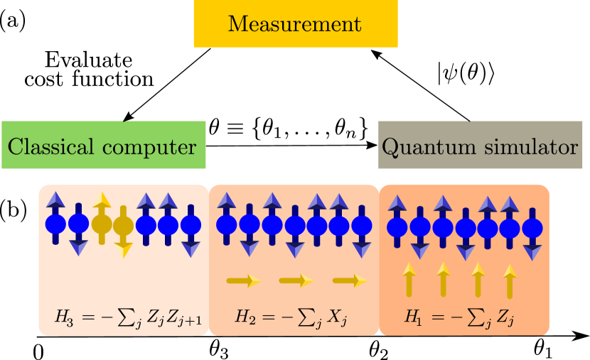
Figure 1: (a) A schematic illustrating a variational quantum-classical optimization routine. The optimization involves $n$ parameters $\theta_{i}$, where $i=1,2,\ldots,n$. For the ansatz in Eq. (1), $n=pM$. (b) The $M=3$-step QAOA algorithm for the preparation of the ground state of the Ising model in both transverse and longitudinal fields, discussed in Sec. IV.

In Ref. Ho and Hsieh, 2019 it was observed that the ground state of the transverse-field Ising model with periodic boundary conditions could be prepared exactly (i.e., with $f=1$) in precisely $p=N/2$ steps, where $N$ is the total number of spins. This was done using the same $M=2$-operator QAOA protocol originally proposed for the MaxCut problem Farhi et al. (2014). This was a surprising result, given that the ground state of the Ising model can be very complex depending on the magnitude of the transverse magnetic field. For instance, at the critical value of the field, the excitation gap goes to zero and the ground state displays logarithmically diverging von Neumann entropy (VNE) of entanglement as a function of subsystem size Calabrese and Cardy (2004). This example demonstrates that the success of QAOA protocol at that circuit depth is not determined by the VNE of the target state. One of the main results of the present paper is to show that a different quantum-information measure called interaction distance Turner et al. (2017) serves as an error-metric for the quality of QAOA state preparation. In the following section, we briefly introduce and review the properties of interaction distance (see also Ref. Pachos and Papic, 2018).

III Interaction distance

Given some density matrix $\rho$, the interaction distance Turner et al. (2017) of $\rho$ is defined as

$$D_{\mathcal{F}}(\rho)\mathrel{\mathop{\mathchar 58\relax}}=\min_{\sigma\in\mathcal{F}}\frac{1}{2}\operatorname*{Tr}\left(\sqrt{(\rho-\sigma)^{2}}\right),$$ (5)

where $\mathcal{F}$ is the manifold of Gaussian density matrices $\sigma$,

$$\mathcal{F} \mathrel{\mathop{\mathchar 58\relax}}=\{\sigma=\frac{1}{Z}e^{-H},Z=\operatorname*{Tr}e^{-H},\text{$H$ is quadratic}\}.$$ (6)

Here, $H$ being quadratic means that it is a free-particle Hamiltonian, e.g., in second quantization, $H=c^{\dagger}hc$ for some matrix $h$ and some set of creation and annihilation operators $\{c_{j}^{\dagger}\}$, $\{c_{j}\}$, with $j\in\{1,...,N\}$.

$D_{\mathcal{F}}$, as defined in Eq. (5), measures distinguishability between a given density matrix $\rho$ and the set of all free-particle density matrices, $\sigma$. Physically, the density matrix $\rho$ can represent a thermal state of the system, in which case it is the standard Boltzmann-Gibbs density matrix when the system is in thermodynamic equilibrium at some temperature $\beta=1/T$. On the other hand, $\rho$ can also be a reduced density matrix which describes the subsystem $A$ of a larger system in the pure state $|\psi\rangle$. In this case, $\rho$ is obtained as the partial trace $\rho_{A}\mathrel{\mathop{\mathchar 58\relax}}=\mathrm{Tr}_{\bar{A}}\;|\psi\rangle\langle\psi|$ over the degrees of freedom of the subsystem $\bar{A}$ complementary to the subsystem $A$.

The reduced density matrix is useful for characterizing properties of $|\psi\rangle$, such as the entanglement entropy of $A$,

$$S_{\mathrm{VNE}}=-\mathrm{Tr}\;\rho_{A}\ln\rho_{A}.$$ (7)

Since $\rho_{A}$ is readily available in numerical simulations, in what follows we focus on $D_{\mathcal{F}}$ evaluated with respect to the reduced density matrix of the model’s ground state.

There is a crucial simplification in evaluating $D_{\mathcal{F}}$ as written in Eq. (5), which was shown in Ref. Turner et al., 2017 using results from  Ref. Markham et al., 2008. The minimization over $\mathcal{F}$ is equivalent to

$$D_{\mathcal{F}}(\rho)=\min_{\{\epsilon_{j}\}}\frac{1}{2}\sum_{k}\mathinner{\!\left\lvert\rho_{k}-\sigma_{k}(\bm{\epsilon})\right\rvert},$$ (8)

where $\rho_{k}$ denote the eigenvalues of $\rho$ in descending order (normalized such that $\sum_{k}\rho_{k}=1$), and

$$\sigma_{k}(\bm{\epsilon})=\frac{1}{Z}e^{-\sum_{j}\epsilon_{j}n_{j}^{(k)}},$$ (9)

where $n_{j}^{(k)}\in\{0,1\}$ is the occupancy number on the $j$th site of the $k$th element of a Fock basis with the energy $\epsilon_{j}$. The normalization $Z$ ensures that $\sum_{k}\sigma_{k}=1$, and we assume that $\sigma_{k}$ are in the same (descending) order as $\rho_{k}$, which is necessary to achieve a minimum in Eq. (8) Markham et al. (2008).

The utility of Eq. (8) is that the value of $D_{\mathcal{F}}(\rho)$ can thus be determined solely from the information of the spectrum $\{-\log\rho_{k}\}$, also known as the “entanglement spectrum” Li and Haldane (2008). Comparing Eq. (5) with Eq. (8), we see that the minimization over all matrices $\sigma\in\mathcal{F}$ was traded for a minimization over scalars $\{\epsilon_{j}\}$. The latter is a much simpler optimization problem, as the number of $\epsilon$ parameters is expected to scale linearly with the system size. Thus, the problem becomes numerically tractable, as the computational complexity is only polynomial in system size $N$ once the spectrum $\{\rho_{k}\}$ is known Turner et al. (2017).

Note that $D_{\mathcal{F}}$ is strictly bounded $0\leq D_{\mathcal{F}}\leq 1$ Meichanetzidis et al. (2018), and states that have $D_{\mathcal{F}}=0$ can be expressed as Gaussian states in terms of some free-particle modes as in Eq. (9). This is, of course, true for unentangled (product states) in the computational basis, but it is also the case for certain entangled states. An example is the ground state of the Ising model in the transverse field, as discussed in the following section. Interestingly, unlike the lower bound, $D_{\mathcal{F}}$ does not seem to saturate its upper bound – it was conjectured that $D_{\mathcal{F}}\leq 3-2\sqrt{2}$ Meichanetzidis et al. (2018). Physical states that realize this upper bound of $D_{\mathcal{F}}$ were identified as ground states of certain types of parafermion chains Meichanetzidis et al. (2018). These states do not have a particularly high value of VNE, but the structure of their entanglement spectrum is as distinct as possible from that of free fermions, in the sense of Eq. (8).

IV Preparing the ground state of the non-integrable quantum Ising model

In this section we present our main findings on the correlation between the success of QAOA state preparation and the interaction distance of the target state. As a toy model, we consider the one-dimensional quantum Ising model in the presence of both transverse and longitudinal fields,

$$H =-\sum_{i=1}^{N}(\pm 1)Z_{i}Z_{i+1}-h_{x}\sum_{i=1}^{N}X_{i}-h_{z}\sum_{i=1}^{N}Z_{i},$$ (10)

where $X_{i}$ and $Z_{i}$ are the standard Pauli matrices on site $i$, and we assume periodic boundary conditions (PBCs) by identifying sites $j+N\equiv j$. The model is either ferromagnetic (FM) or antiferromagnetic (AFM) depending on whether the coupling of the first term is chosen to be $+1$ or $-1$, respectively. The Ising models in Eqs. (10) serve as a useful laboratory for studying a number of phenomena in condensed matter physics Dutta et al. (2015); Coldea et al. (2010); Morris et al. (2014).

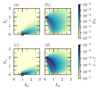
Figure 2: Top row: Interaction distance for the ground state of FM (a) and AFM (b) model in Eq. (10) as a function of fields $h_{x}$ and $h_{z}$. Bottom row: the infidelity $1-f$ of the QAOA protocol for the FM (c) and AFM model (d). See text for the details of the QAOA protocol. All data is for system size $N=8$ using PBCs. Red dot denotes the critical point of the FM model, while the red line is the critical line in the AFM model according to Ref. Ovchinnikov et al., 2003.

The properties of the ground state of the model in Eq. (10) are insensitive to the sign of the FM/AFM coupling in the absence of longitudinal field $h_{z}$. However, once $h_{z}>0$, the phase diagram is substantially different for the two models. The FM model has a critical point at $(h_{x},h_{z})=(1,0)$, while the AFM model has a critical line connecting the point $(h_{x},h_{z})=(1,0)$ with the point $(h_{x},h_{z})=(0,2)$. The critical line is not known analytically, but it has been determined numerically using density-matrix renormalization group simulations in Ref.  Ovchinnikov et al., 2003. In both cases, the limit of purely transverse field ($h_{z}=0$) is particularly important. Along this line, the Hamiltonian is diagonal when written in terms of free fermions after performing a combination of the Jordan-Wigner and Bogoliubov transforms Pfeuty (1970).

The phase diagrams of the FM and AFM models diagnosed by the value of $D_{\mathcal{F}}$ in their ground state are shown in Fig. 2(a)-(b), respectively. The ground state of the Hamiltonian in Eq. (10) is obtained numerically using exact diagonalization, and its entanglement spectrum is computed by partitioning the system into two equal halves. From the entanglement spectrum, $D_{\mathcal{F}}$ is evaluated by numerical optimization following Eq. (8) . For both models, $D_{\mathcal{F}}$ is found to be zero (to machine precision) when $h_{z}=0$, regardless of the value $h_{x}$. Away from this line, $D_{\mathcal{F}}$ is a sensitive indicator of interaction effects and changes by many orders of magnitude depending on the location in the phase diagram. For example, in the FM model, $D_{\mathcal{F}}$ exhibits a sharp peak just off the free Ising critical point, $(h_{x}=1,h_{z}=0)$. While the Ising critical point is described by the free Ising conformal field theory Francesco et al. (2012) and thus it has $D_{\mathcal{F}}=0$, the properties of this CFT change dramatically once $h_{z}$ field is introduced Zamolodchikov (1989). This is consistent with the fermionic picture, where the $h_{z}$ field introduces long-range interaction between fermions after the Jordan-Wigner transformation, which makes the system’s ground state highly interacting. Somewhat surprisingly, away from the critical point, the value of $D_{\mathcal{F}}$ sharply decays to values as low as $\sim 10^{-7}$, even though the interaction is comparable in magnitude to other terms in the Hamiltonian. This implies that there are large regions of the phase diagram where the ground state of the system is effectively free-fermion-like, even though the Hamiltonian itself is “interacting”. On the other hand, the AFM model features a critical line that extends from the free Ising critical point $(h_{x}=1,h_{z}=0)$. While $D_{\mathcal{F}}=0$ at $(h_{x}=1,h_{z}=0)$, the value of interaction distance progressively increases along the critical line towards the interior of the phase diagram – see Fig. 2(b).

Next, we explore how to prepare the ground state of Eq. (10) using QAOA for arbitrary values of fields $h_{x}$ and $h_{z}$. To this end, we have found it necessary to employ a $M=3$-step QAOA protocol from Eq. (II) with the operators

$$H_{1} = -\sum_{i=1}^{N}Z_{i},$$ (11)

$$H_{2} = -\sum_{i=1}^{N}X_{i},$$ (12)

$$H_{3} = -\sum_{i=1}^{N}Z_{i}Z_{i+1},$$ (13)

which satisfy $\pm H_{3}+h_{x}H_{2}+h_{z}H_{1}=H$, see the illustration in Fig. 1(b). The initial state of the protocol is taken to be the ground state of $H_{2}$, i.e., all spins polarized along $x$-direction, $|\psi_{\mathrm{init}}\rangle=|\rightarrow\ldots\rightarrow\rangle$. Since Pauli matrices are involutions, these operators $H_{j}$ satisfy $e^{-i(\theta+\pi)H_{j}}=\pm e^{-i\theta H_{j}}$, so in what follows we restrict the representation of $\bm{\theta}$ angles to $[0,\pi[$ interval. We further restrict the angle $\theta_{p,3}$ associated with $H_{3}$ to the $[0,\frac{\pi}{2}[$ interval, since

$$\prod_{i}^{N}e^{i(\theta+\frac{\pi}{2})Z_{i}Z_{i+1}} \propto \prod_{i=1}^{N}Z_{i}Z_{i+1}\prod_{i=1}^{N}e^{i\theta Z_{i}Z_{i+1}}$$ (14)

$$\propto \prod_{i=1}^{N}e^{i\theta Z_{i}Z_{i+1}}.$$

The initial guesses for the angles were determined sequentially as $p$ is increased, following the method in Appendix B1 of Ref. Zhou et al., 2019. For minimizations involved in both QAOA and $D_{\mathcal{F}}$ we use a basinhopping algorithm with a Metropolis acceptance criterion Wales and Doye (1997), as implemented in the Python package scipy.optimize.basinhopping. This is a global strategy that performs multiple minimizations, taking as the initial condition for the next minimization the stochastically perturbed result of the previous one. This allows us to avoid the local minima associated with the rugged landscapes of both QAOA and $D_{\mathcal{F}}$, as discussed further in Sec. VI. This, however, was not enough to completely eliminate local minima, and all the data presented here required two additional rounds of minimization. Each of these consisted in running the basinhopping algorithm across the phase diagram again, this time using as initial value for each point the optimal values of each of the adjacent points from the previously obtained data, and keeping the minimum value found.

Note that our protocol in Eqs. (11)-(13) is a generalization of the one considered in Ref. Ho and Hsieh, 2019, which was restricted to the purely transverse field ($h_{z}=0$) and made use of a $M=2$-step ansatz with only $H_{2}$ and $H_{3}$. In that case, both the Hamiltonian and the protocol conserve the total fermion parity, generated by $P=\prod_{i}X_{i}$. This symmetry is broken once the $z$-field is introduced and the ground state acquires a non-zero magnetization $\braket{\psi}{\sum_{i}Z_{i}}{\psi}\neq 0$. While it is easy to come up with a two-step protocol that does not conserve parity, we have not been able to find one that accurately prepares the ground state for general values of $(h_{x},h_{z})$, thus we introduced a third operator into the QAOA protocol.

In Figs. 2(c)-(d) we present results of the QAOA protocol across the phase diagram $(h_{x},h_{z})$. The color scale in Fig. 2(c)-(d) shows the infidelity $1-f$ obtained after fixed $p=\frac{N}{2}$ steps of QAOA. We observe that this metric of ground state preparation looks remarkably similar to the behavior of $D_{\mathcal{F}}$ in Figs. 2(a)-(b). In particular, we recover $f=1$ when $h_{z}=0$ Ho and Hsieh (2019), while the QAOA no longer finds an exact ground state when $h_{z}>0$. Nevertheless, it approximates the ground state very closely when $D_{\mathcal{F}}$ is small. Once again, it is easy to see that in this case there is no clear relation between QAOA’s $1-f$ and the VNE of the ground state. For example, in the FM model, the VNE should be largest at the critical point; further, as adding $h_{z}$ opens a gap in the spectrum, increasing this parameter should reduce the VNE, as its scaling changes from logarithmic divergence with system size to an area law. However, from the point of view of QAOA, we find precisely the opposite: it is harder to prepare the state with some small amount of $h_{z}$ compared to $h_{z}=0$.

Examining the optimal angles found at each point of the phase diagram of both the FM/AFM Ising models when running the protocol in Eqs.(11)-(13), we found no continuous variation of the angles across the phase diagram of the kind, e.g., in Ref. Zhou et al., 2020. However, we found that the optimal angles $\theta_{j,1}$ had a striking tendency to be very close to multiples of $\frac{\pi}{2}$ (see Fig. 8 in the Appendix). This suggests that the Hamiltonian $H_{1}$ has a restricted role in the evolution, and that the symmetry which led us to use a 3-step protocol could perhaps be broken in a simpler way. This property could be exploited by having the initial guess be close to multiples of $\frac{\pi}{2}$ through an ansatz, or by giving higher weight to regions close to these two points ($0$ and $\frac{\pi}{2}$) in the minimization algorithm.

In Fig. 3, we show a scatter plot of $D_{\mathcal{F}}$ vs. $1-f$ from the data extracted from phase diagrams such as in Fig. 2, but using different numbers of QAOA steps $p$, indicated in the legend. In both FM and AFM models, we expect correlation between $D_{\mathcal{F}}$ and $1-f$ around $p=\frac{N}{2}$. This correlation peak is relatively broad as $p$ is increased further. Eventually, as $p\to\infty$, we expect states to be exactly prepared and this correlation to break down, as in this limit our QAOA protocol should have the same power as quantum annealing with an arbitrary schedule Mbeng et al. (2019a). In the opposite limit, as $p\to 1$, we expect that the variational method, in general, is not powerful enough for a correlation to emerge. However, in special cases such as the FM model, we see that $D_{\mathcal{F}}$ and $1-f$ are correlated even at lower $p$. We compute the Pearson correlation coefficients for the data in Fig. 3 and plot them in Fig. 9 of the appendix; as expected, the Pearson coefficient jumps to a value close to 1 around $p=\frac{N}{2}$.

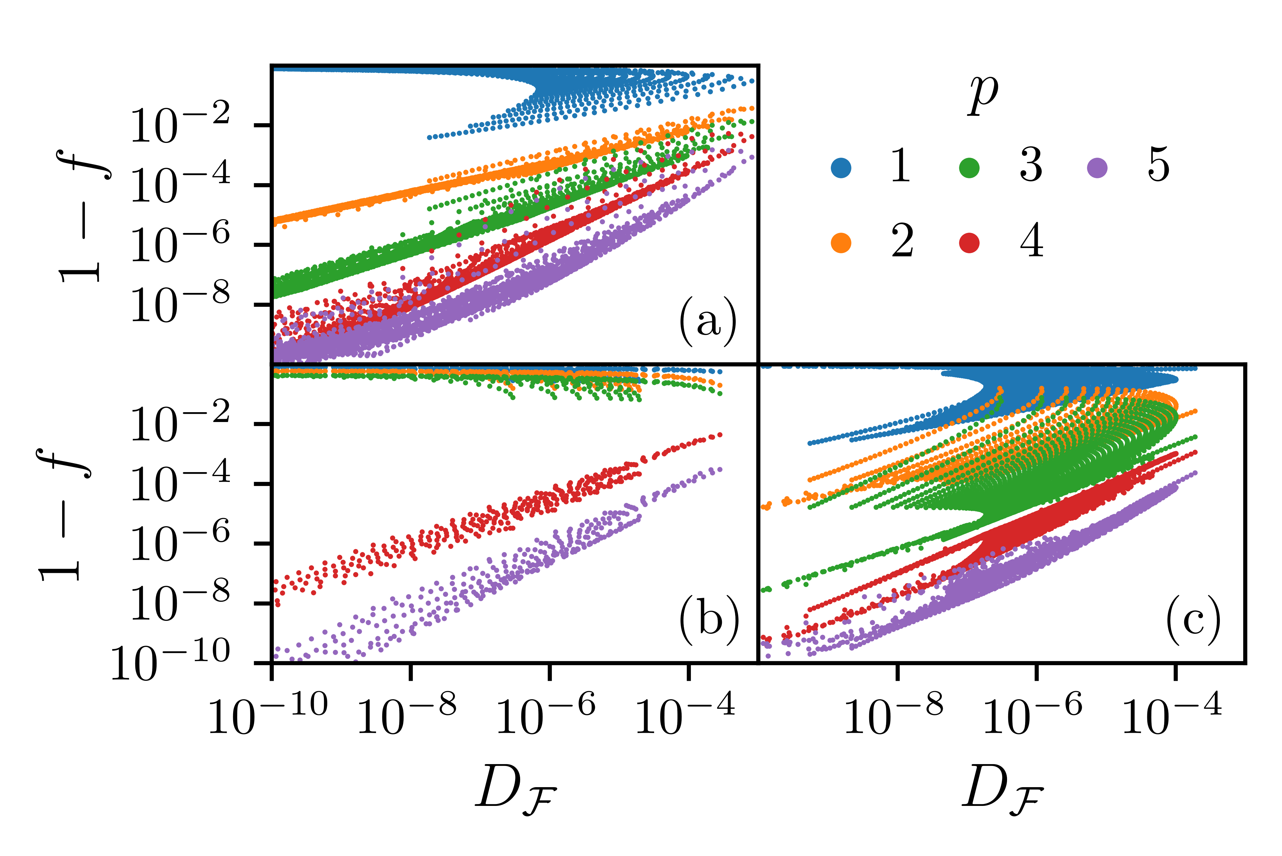
Figure 3: (a) Scatter plot of interaction distance $D_{\mathcal{F}}$ against QAOA’s $1-f$ for the FM Ising model from Fig. 2(c). (b)-(c): Analogous plot for the AFM Ising model in Fig. 2(d), where the data points are taken either below (b) or above (c) the critical line. Data is for $N=8$ spins with PBCs and different values of $p$ indicated in the legend.

For the AFM Ising model in Fig. 3(b)-(c), we found that the correlation between $D_{\mathcal{F}}$ and $1-f$ follows a different slope in the two phases of the AFM model separated by the critical line in Fig. 2(d). In particular, the behavior in the ordered phase of the model, Fig. 3(b), clearly illustrates that the correlation between $D_{\mathcal{F}}$ and $1-f$ only starts to emerge around $p=N/2$. Moreover, different slopes of the correlation in the two phases suggest that by carefully examining the correlation between these two metrics one could infer about the existence of different phases in models with unknown phase diagrams.

V Relation between QAOA and interaction distance

In Sec. IV, we have established numerically a correlation between $D_{\mathcal{F}}$ and the success of QAOA protocols. This suggests that the protocol’s success depends on how close to being Gaussian (in the sense of Eq. (6)) the target ground state is. In this section, we support these numerical observations by analytic arguments.

As mentioned in Sec. IV, the angle $\theta_{j,1}$ associated with the operator Eq. (11) is found to cluster around either $0$ or $\frac{\pi}{2}$. Now, note that a shift of $\pi/2$ in the $\theta_{j,1}$ part of the protocol results in an overall parity flip, as easily seen from the following sequence of identities:

$$\exp\left(i\left(\theta_{j,1}+\frac{\pi}{2}\right)\sum_{i}Z_{i}\right)\exp\left(i\theta_{j,2}\sum_{i}X_{i}\right)$$

$$=\exp\left(i\theta_{j,1}\sum_{i}Z_{i}\right)\prod_{i}Z_{i}\exp\left(i\theta_{j,2}\sum_{i}X_{i}\right)$$

$$=\exp\left(i\theta_{j,1}\sum_{i}Z_{i}\right)\exp\left(i\theta_{j,2}\sum_{i}-X_{i}\right)\prod_{i}Z_{i}.$$

Further,

$$\prod_{i}Z_{i}\ket{\rightarrow...\rightarrow}=\ket{\leftarrow...\leftarrow},$$

where $|\rightarrow\rangle$, $|\leftarrow\rangle$ denote eigenstates of $X$. This implies that, if we have the freedom of choosing either $\ket{\rightarrow...\rightarrow}$ or $\ket{\leftarrow...\leftarrow}$ as the initial state, we can restrict, without loss of generality, all angles $\theta_{j,1}$ to an interval of length $\pi/2$. Since these angles are clustered around $0$ and $\pi/2$ as shown in Fig. 8 of the Appendix, they can all be mapped to be close to 0.

Next, note that since both initial states are product states, they are also Gaussian states. Moreover, the evolution under the unitaries generated by $H_{3}$ and $H_{2}$ maps Gaussian states into Gaussian states, while the evolution under $H_{1}$ spoils this property. However, for $\theta_{j,1}$ close to $0$, the evolution under $H_{1}$ introduces only a small, perturbative deviation from a Gaussian state. This heuristically accounts for the high correlation of QAOA success with interaction distance of the target state, as the states prepared by QAOA are close to being free. As $p$ gets larger, more perturbations are possible and the success of the QAOA increases. At a fixed $p$, the success of QAOA is related to the distance of the target state from the Gaussian state manifold.

We conclude that there is a practical limitation to the “natural” QAOA protocol proposed in Sec. IV, which was obtained as a Trotter splitting of the Hamiltonian in Eq. (10) into its translation invariant components: the protocol is unable to prepare ground states that are far from being Gaussian (as measured by interaction distance). This limitation is fundamentally related to the probability spectrum of the target state, i.e., the eigenvalue spectrum of its reduced density matrix. Indeed, when performing QAOA using as a cost function the relative entropy Nielsen and Chuang (2010) between the probability spectra of the trial state and of the target state, one finds heat maps similar to those in Fig. 2 (data not shown). Thus, there is a correlation between QAOA and $D_{\mathcal{F}}$, even though the former minimizes the overlap of two vectors, while the latter employs a minimization using the probability spectrum of the subsystem’s reduced density matrices.

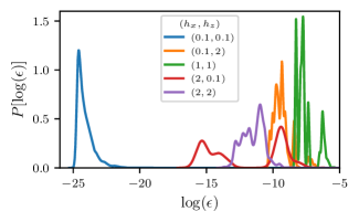
Figure 4: Probability distribution function $P(\log(\epsilon))$ of QAOA outcomes on 10000 uniformly generated initial angles having as target the ground state of the points in $S$. Data is for system size $N=8$ and $p=4$, with the protocol in Eqs. (13)-(11).

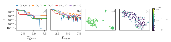
Figure 5: Minimization landscape in the AFM Ising model. (a) Relative energy $\epsilon$ vs. $T_{\leq\max}$ for different points in $S$. (b) Relative energy $\epsilon$ vs. $T_{=\max}$ for different points in $S$. (c) t-SNE graph for 500 random angle samples taken at $(h_{x},h_{z})=(1,1)$ and $T_{=\max}=1$. (d) t-SNE graph for 500 random angle samples taken at $(h_{x},h_{z})=(1,1)$ and $T_{=\max}=8$. All data is for system size $N=6$ and $p=3$. Color scale in (c), (d) represents the value of $\epsilon$.

VI Minimization landscape

In this section, we explore the minimization landscape of the optimization problem studied in Sec. IV for the AFM Ising model (we reached qualitatively similar conclusions in the FM model). The target state in the cost function is taken to be the ground state of the Hamiltonian at a set of representative points in the ($h_{x}$, $h_{z}$) phase diagram, $S=\{(0.1,0.1),(0.1,2),(1,1),(2,0.1),(2,2)\}$. These points are drawn from regions of both “hard” and “easy” state preparation according to Fig. 2. Here, we use the rescaled relative energy, defined in Eq. (3), instead of the quantum infidelity.

In Fig. 4 we first look at the probability distribution function for $\log\epsilon$ in selected points $S$. We generate a sample of $10^{4}$ initial $\theta$ angles, drawn from a uniform distribution in the $[0,\pi[$ interval. The distribution of $\log\epsilon$ gives us insight about the structure of the landscape. A sharply-defined distribution of $\log\epsilon$ is only obtained in the case where $h_{x}=h_{z}=0.1$, with the peak at $\epsilon$ close to 0. The mean of the distribution shifts to large values of $\epsilon$ upon approaching the critical line, e.g., at $h_{x}=h_{z}=1$. In addition to the shift of the mean, the distribution also develops multiple peaks corresponding to local minima. At other points in the phase diagram, such as $h_{x}=h_{z}=2$, the separate minima form a smooth curve with larger variance. Finally, in some cases like $h_{x}=2$, $h_{z}=0.1$, we observe a clear bimodal distribution of the minima. Thus, the distribution of minima varies considerably across the phase diagram and, generally, has multiple peaks.

A systematic investigation of the nature of the landscape of a related minimization problem was performed in Refs. Bukov et al., 2018; Day et al., 2019; Liang et al., 2020 using a discretized adiabatic state preparation protocol. In these works, the behavior of the minimization landscape was examined as a function of the total allowed time for the protocol. It was found Bukov et al. (2018); Day et al. (2019) that there are distinct “phases” associated with different intervals for the total allowed time. Particularly, at intermediate times, there is a glassy phase presenting with multiple clusters of minima where the minimization becomes difficult. Following Refs. Bukov et al., 2018; Day et al., 2019, we have probed the nature of the minimization landscape in our models and using our QAOA protocol when the total time $T({\bm{\theta}})=\sum_{i=1}^{p}\sum_{j=1}^{M}\theta_{i,j}$ is restricted. We impose this restriction in two different ways. First, we allow $T({\bm{\theta}})$ to be less than or equal to some maximum total time $T_{\leq\max}$, which can be easily achieved by constraining the allowed interval for each $\theta_{i,j}$ angle in our protocol. The second method is to demand $T({\bm{\theta}})$ to be exactly equal to a given total time $T_{=\max}$. The results of these two approaches are contrasted in Fig. 5(a) and (b).

In Fig. 5(a) we see that, as expected, as $T_{\leq\max}$ increases, $\epsilon$ decreases. Perhaps surprisingly, this occurs in a very clear step-wise fashion, suggesting that there are discrete values of $T_{\leq\max}$ that show significant improvement in state preparation. By contrast, in Fig. 5(b) we see that as $T_{=\max}$ increases, the behavior of $\epsilon$ is more erratic, indicating that there are discrete, optimum values of $T$ for which states can be prepared under this restriction. This shows that the protocol can not accommodate non-optimal values $T_{=\max}$, that is, there is no way for the protocol to continuously ”stall” and wait, ”wasting time” so as to emulate the last optimal value of $T_{=\max}$. The protocol can, however, ”stall” in discrete values of $\pi$, due to the symmetry in the angles. A consequence of this seems to be the peaks and troughs pattern in the graphs in Fig. 5(b), which show an irregular pattern. This contrasts with the results in Ref. Bukov et al., 2018; Day et al., 2019, which display an almost monotonically increasing success in state preparation as $T_{=\max}$ increases.

Next, we took 500 random angle samples restricted to either $T_{=\max}$ or $T_{\leq\max}$ and ran QAOA with target state coming from the ground state at each of the representative points in $S$. Here, we have used the L-BFGS local optimization algorithm, as implemented in the scipy Python package, to perform the minimization. In order to plot the high-dimensional minimization landscape, we have used t-SNE Maaten and Hinton (2008), a dimensionality-reduction algorithm for data visualization that embeds high dimensional data in a space with lower dimension while preserving the relative position of the data points. Performing t-SNE on these samples, we find that, for $T_{\leq\max},T_{=\max}<1$, there exists clustering of minima, although some of the clusters are significantly less compact than others – see Fig. 5(c). For $T_{\leq\max},T_{=\max}>1$, the clustering rapidly disappears, first for the $T_{\leq\max}$ restriction and then for the $T_{=\max}$ restriction – an example of the latter is shown in Fig. 5(d) for $T_{=\max}=8$. This indicates that QAOA, which usually does not place restrictions on the values of $\theta$ angles and therefore implicitly operates in the large-$T$ regime, does not display a glassy phase in its minimization landscape as found for a different protocol in Refs.  Bukov et al., 2018; Day et al., 2019.

VII Conclusions

In this paper we have investigated the preparation of ground states of non-integrable quantum models using QAOA. Our motivation was to identify physical properties of the state that have an impact on its preparation, thereby allowing us to bound the relative success of QAOA. While this task appears challenging for rigorous analytical treatment, we have numerically demonstrated a correlation between interaction distance and the success of the QAOA protocols in several variants of the quantum Ising model. This suggests that, in these models, states which are far from free, as measured by interaction distance, are harder to prepare, i.e., in order to prepare states with larger interaction distance, QAOA needs higher values of $p$ to achieve the same degree of success as for states with lower interaction distance and lower $p$. We have also performed an analysis of the landscape associated with the QAOA optimization problem. We have found that there are several local minima associated with this landscape, though they are spread out and show no distinctive clustering. Limiting the total allowed QAOA time did not alter this landscape significantly for total time $T\gtrsim 1$.

One of the applications of our results is that theoretical insight into the closest free states representing the target state can be gained by using the experimentally obtained QAOA ansatz and setting the small $\theta_{j,1}$ angles to be zero. The absence of the glassy phase in the minimization landscape implies that the natural QAOA protocols constructed here do not lead to a NP-hard optimization problem and the time to find optimal angles should scale polynomially with the system size.

VIII Acknowledgements

We acknowledge useful discussions with Chris Self, Christopher Turner, and Marin Bukov. This work was supported by EPSRC grant EP/R020612/1. Statement of compliance with EPSRC policy framework on research data: This publication is theoretical work that does not require supporting research data.

Appendix A Three-spin Ising model

Here we demonstrate that our findings from the main text also apply in a different model featuring three-spin interactions. The model is defined by the Hamiltonian

$$H =-\sum_{i=1}^{N}Z_{i}Z_{i+1}Z_{i+2}-h_{x}\sum_{i=1}^{N}X_{i}-h_{z}\sum_{i=1}^{N}Z_{i},$$ (15)

where, again, $X_{i}$ and $Z_{i}$ are the standard Pauli matrices on site $i$, and we assume PBCs. The critical behavior of this model is in the same universality class as the two-dimensional classical three-state Potts model. The phase diagram of the model has been mapped out in Ref. Penson et al., 1988 (see also Ref. Iglói, 1989 for further generalisations of the model). In the $h_{x}>0$, $-3\leq h_{z}<0$ region, it contains a critical line connecting $(h_{x},h_{z})=(0,-3)$ to $(h_{x},h_{z})=(1,0)$. Below that critical line, there exists a threefold ground state degeneracy, while above it the ground state is unique.

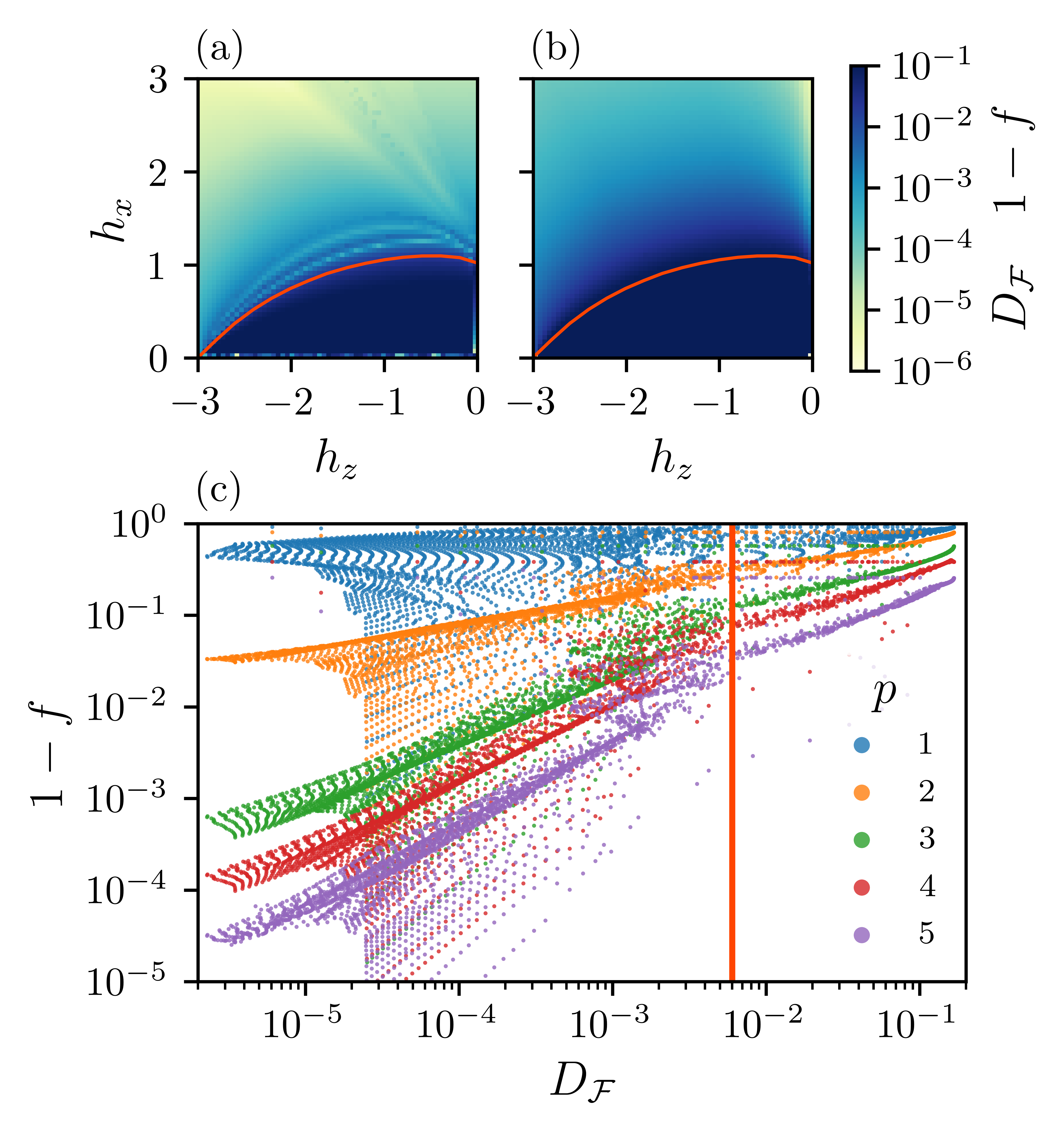
Figure 6: Top row: Interaction distance for the 3-spin Ising model in Eq. (15) as a function of fields $h_{x}$ and $h_{z}$ (a) and the infidelity $1-f$ of the QAOA protocol (b). The QAOA protocol is based on Eqs. (11), (12), (17). All data is for system size $N=9$ using PBCs. Red line is the critical line in the 3-spin Ising model according to Ref. Penson et al., 1988 Bottom row: Scatter plot of $D_{\mathcal{F}}$ against $1-f$ for the 3-spin Ising model, system size $N=9$ and different values of $p$ indicated in the legend. Vertical red line, drawn heuristically, separates the data belonging to the phase above and below the critical line (respectively to the left and right of the vertical line).

.

The motivation for studying the model in Eq. (15) is that its ground state is expected to be more strongly interacting and have a higher value of $D_{\mathcal{F}}$. For example, unlike the FM/AFM models in Eq. (10), the ground state of the model in Eq. (15) cannot be obtained in closed form using the Jordan-Wigner and/or Bogoliubov transformation (apart from classical line, $h_{x}=0$). Moreover, the 3-fold ground state degeneracy in the ordered phase gives rise to an approximate 3-fold degeneracy of the entanglement spectrum, as generally found in “symmetry-protected topological phases” Pollmann et al. (2010b). This can be understood by picking a point $(h_{x}=0,h_{z}=-1)$, where the exact ground state of the system (with zero momentum under translation) is given by

$$|\psi_{0}\rangle=\frac{1}{\sqrt{3}}(|\uparrow\downarrow\downarrow\uparrow\downarrow\downarrow\ldots\rangle+|\downarrow\uparrow\downarrow\downarrow\uparrow\downarrow\ldots\rangle+|\downarrow\downarrow\uparrow\downarrow\downarrow\uparrow\ldots\rangle).\quad\quad$$ (16)

The corresponding entanglement spectrum is given by $\rho_{k}=\{\frac{1}{3},\frac{1}{3},\frac{1}{3},0,0,\ldots\}$. This is the type of entanglement spectrum that gives $D_{\mathcal{F}}=\frac{1}{6}$, a value close to the upper bound $3-2\sqrt{2}$ Meichanetzidis et al. (2018). The same spectrum is obtained in the $\mathbb{Z}_{3}$ parafermion model at its fixed point Mong et al. (2014). An approximate 3-fold degeneracy in the entanglement spectrum persists throughout the ordered phase of the model, thus we expect the ground state throughout this phase to be more difficult to prepare using QAOA compared to the disordered phase.

The comparison between $D_{\mathcal{F}}$ and QAOA for the model in Eq. (15) is shown in Fig. 6. The QAOA protocol was chosen such that $H_{1}$ and $H_{2}$ are defined as in Eqs. (11)-(12), but for $H_{3}$ we use

$$H_{3}=-\sum_{i=1}^{N}Z_{i}Z_{i+1}Z_{i+2}.$$ (17)

Note that this protocol also satisfies $H_{3}+h_{x}H_{2}+h_{z}H_{1}=H$. We have found that, like the two-spin Ising model, the success of the protocol also correlates well with interaction distance, as we see in the top row of Fig. 6. Here, as in Section IV, minimizations are done using a basinhopping algorithm, and the results required two additional rounds of minimization. Moreover, we find correlation between $D_{\mathcal{F}}$ and $1-f$ for several values of $p$, as shown in the bottom row of Fig. 6. As before, the data in the bottom row of Fig. 6 was obtained by sampling across the entire phase diagram in the top row of Fig. 6.

It worth noting that we can prepare the ground state in Eq. (16) exactly by choosing the protocol $H_{2}=-\sum_{j}Z_{j-1}Z_{j}Z_{j+1}$ and $H_{1}=-\sum_{j}(X_{j}X_{j+1}+Y_{j}Y_{j+1})$, while the initial state is the ground state of $H_{2}$ in the sector with magnetization $-N/3$, as this is the sector where the states $\{\ket{\uparrow\downarrow\downarrow...},\ket{\downarrow\uparrow\downarrow...},\ket{\downarrow\downarrow\uparrow...}\}$ live. It can be verified that this protocol prepares the exact ground state in Eq. (16) in $N/2$ steps. Moreover, supplementing the protocol with a third operator, $H_{3}=-\sum_{j}X_{j}$, leads to good results across the entire phase with the 3-fold ground-state degeneracy. However, the infidelity $1-f$ of the latter protocol does not capture the phase transition in a way that the protocol [Eqs.(12), (11), (17)] does. Moreover, the initial state is more difficult to prepare in this case, unlike the product state of spins in our protocol.

Similar to the models studied in Sec. IV, we found no continuous variation of angles in the three-spin Ising model, and the angles $\theta_{j,1}$ tended to be close to multiples of $\pi/2$ (see Fig. 8). However, in this case the heuristic arguments of of Sec. V do not directly apply as the Gaussianity of the protocol is broken by the triple spin interaction term (17). It is an interesting open problem to analytically explain the approximate Gaussianity in this case.

Appendix B Cluster Ising model

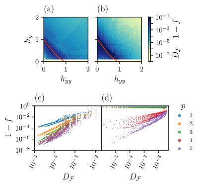
Figure 7: Top row: Interaction distance for the cluster Ising model in Eq. (18) as a function of $h_{yy}$ and $h_{y}$ (a) and the infidelity $1-f$ of the QAOA protocol (b). All data is for system size $N=8$ with periodic boundary conditions. Red line is reproduced from Ref. Verresen et al., 2017. Bottom row: Scatter plot of $D_{\mathcal{F}}$ against $1-f$ for the cluster Ising model, system size $N=8$ and different values of $p$ indicated in the legend. Panel (c) shows points above the critical line while (d) shows points below it.

As another example illustrating the versatility of our method, we consider the cluster Ising model, which has recently attracted attention both in the context of quantum information Pachos and Plenio (2004); Smacchia et al. (2011) and symmetry-protected topological phases Verresen et al. (2017). The model is defined in terms of Pauli matrices (assuming periodic boundary conditions) as:

$$H=-\sum_{i=1}^{N}X_{i-1}Z_{i}X_{i+1}-\sum_{i=1}^{N}h_{yy}Y_{i}Y_{i+1}+\sum_{i=1}^{N}h_{y}Y_{i}.\quad\quad$$ (18)

When the field $h_{y}=0$, the model can be solved using a combination of Jordan-Wigner/Bogoliubov transformations Smacchia et al. (2011), but for general values of $h_{y}$ the model is not solvable. The model has a critical line described by conformal field theory with central charge $c=3/2$, connecting points $(h_{yy}=1,h_{y}=0)$ and $(h_{yy}=0,h_{y}=1)$. The critical line has been mapped out using density-matrix renormalisation group calculations in Ref. Verresen et al., 2017.

As seen in Fig. 7(a)-(b), both QAOA and $D_{\mathcal{F}}$ are highly sensitive to the critical line, just like we have previously seen in the AFM Ising and 3-spin Ising models. Despite small system size, the critical behavior is in good qualitative agreement with results of Ref. Verresen et al., 2017. The QAOA protocol in Fig. 7 has been defined by splitting $H$ into its three components, $H_{3}=-\sum_{i=1}^{N}X_{i-1}Z_{i}X_{i+1}$, $H_{2}=-\sum_{i=1}^{N}Y_{i}Y_{i+1}$, $H_{1}=-\sum_{i=1}^{N}Y_{i}$. For the initial state, one can choose the ground state of $H_{1}$. However, with this initial state, the convergence of the optimization below the critical line was found to be very slow; instead, the convergence is considerably more robust if we use as initial state the ground state of $H_{2}$ in this regime. In producing the phase diagram in Fig. 7(b) we have run two sweeps of QAOA starting in either of these initial states, and plotting the smaller value of the obtained $1-f$.

It is worth noting that the line with $h_{y}=0$ is prepared exactly (to machine precision) in $p=N/2$ steps using the 2-step protocol involving only $H_{3}$ and $H_{2}$, similar to the case of the transverse field Ising model. Moreover, there is correlation between $D_{\mathcal{F}}$ and $1-f$ across each of the two phases of the model, as illustrated in Fig. 7(c)-(d).

Appendix C Additional data

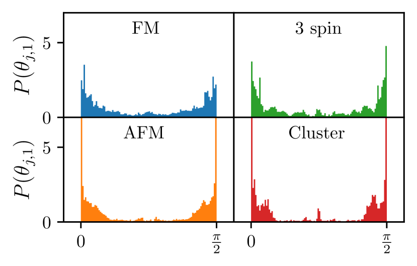
Figure 8: Distribution of angles $\theta_{j,1}$ associated with the Hamiltonian in Eq. (11) in QAOA evolution across phase diagrams of FM/AFM, 3-spin and cluster Ising models in Eqs. (10), Eq. (15) and Eq. (18). Data is for system size $N=8$ with the exception of $N=9$ for the 3-spin Ising model. In all the plots, $p=4$.

This section contains some additional results that support the conclusions in the main text. Fig. 8 shows the distribution of the angles $\theta_{j,1}$ associated to the “interacting” part of the Hamiltonian, i.e., $H_{1}$ in Eq. (11) in the QAOA protocol. As claimed in Sections IV-V, these angles tend to be close to $0$ or $\frac{\pi}{2}$, which is clearly seen in the figure for all the models considered in this paper.

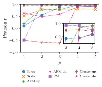
Figure 9: Pearson correlation coefficients as a function of $p$ for the data in Figures 3, 6(c) and  7(c). Labels ”up” and ”dn” denote data above and below the critical line of the corresponding model, respectively. The inset zooms in on the top-right corner of the plot.

Finally, we compute the Pearson correlation coefficients for the data in Figs 3, 6(c) and  7(c)-(d), and plot them in Fig. 9. We see that the Pearson coefficient jumps to a value close to 1, indicating direct correlation. As explained in the main text, we expect this to mark the beginning of a broad plateau where the Pearson coefficient remains close to 1, until it eventually starts to drop at larger values of $p$. The reason for this decay is the exact preparation of the state in the limit $p\to\infty$ for the protocol considered here. Conversely, in the limit $p\to 1$, we expect the variational ansatz is not sufficiently powerful for the correlation to emerge.

References

- Peruzzo et al. (2014) Alberto Peruzzo, Jarrod McClean, Peter Shadbolt, Man-Hong Yung, Xiao-Qi Zhou, Peter J. Love, Alán Aspuru-Guzik, and Jeremy L. O’Brien, “A variational eigenvalue solver on a photonic quantum processor,” Nature Communications 5, 4213 (2014).
- Farhi et al. (2014) Edward Farhi, Jeffrey Goldstone, and Sam Gutmann, “A Quantum Approximate Optimization Algorithm,” arXiv:1411.4028 [quant-ph] (2014).
- Preskill (2018) John Preskill, “Quantum Computing in the NISQ era and beyond,” Quantum 2, 79 (2018).
- Lloyd (2018) Seth Lloyd, “Quantum approximate optimization is computationally universal,” arXiv:1812.11075 [quant-ph] (2018).
- Morales et al. (2019) Mauro E. S. Morales, Jacob Biamonte, and Zoltán Zimborás, “On the Universality of the Quantum Approximate Optimization Algorithm,” arXiv:1909.03123 [math-ph, physics:quant-ph] (2019).
- Farhi et al. (2019) Edward Farhi, Jeffrey Goldstone, Sam Gutmann, and Leo Zhou, “The Quantum Approximate Optimization Algorithm and the Sherrington-Kirkpatrick Model at Infinite Size,” arXiv:1910.08187 [cond-mat, physics:quant-ph] (2019).
- Vikstål et al. (2019) Pontus Vikstål, Mattias Grönkvist, Marika Svensson, Martin Andersson, Göran Johansson, and Giulia Ferrini, “Applying the Quantum Approximate Optimization Algorithm to the Tail Assignment Problem,” arXiv:1912.10499 [quant-ph] (2019).
- Hadfield et al. (2019) Stuart Hadfield, Zhihui Wang, Bryan O’Gorman, Eleanor Rieffel, Davide Venturelli, and Rupak Biswas, “From the Quantum Approximate Optimization Algorithm to a Quantum Alternating Operator Ansatz,” Algorithms 12, 34 (2019).
- Oh et al. (2019) Young-Hyun Oh, Hamed Mohammadbagherpoor, Patrick Dreher, Anand Singh, Xianqing Yu, and Andy J. Rindos, “Solving Multi-Coloring Combinatorial Optimization Problems Using Hybrid Quantum Algorithms,” arXiv:1911.00595 [quant-ph] (2019).
- Sundar et al. (2019) Bhuvanesh Sundar, Roger Paredes, David T. Damanik, Leonardo Dueñas-Osorio, and Kaden R. A. Hazzard, “A quantum algorithm to count weighted ground states of classical spin Hamiltonians,” arXiv:1908.01745 [quant-ph] (2019).
- Ho and Hsieh (2019) Wen Wei Ho and Timothy H. Hsieh, “Efficient variational simulation of non-trivial quantum states,” SciPost Phys. 6, 29 (2019).
- Ho et al. (2019) Wen Wei Ho, Cheryne Jonay, and Timothy H. Hsieh, “Ultrafast variational simulation of nontrivial quantum states with long-range interactions,” Phys. Rev. A 99, 052332 (2019).
- Wauters et al. (2020) Matteo M. Wauters, Glen Bigan Mbeng, and Giuseppe E. Santoro, “Polynomial scaling of QAOA for ground-state preparation: taming first-order phase transitions,” arXiv:2003.07419 [cond-mat, physics:quant-ph] (2020).
- (14) Nicolas Vogt, Sebastian Zanker, Jan-Michael Reiner, Thomas Eckl, Anika Marusczyk, and Michael Marthaler, “Preparing symmetry broken ground states with variational quantum algorithms,” 2007.01582 .
- Zhu et al. (2019) D. Zhu, S. Johri, N. M. Linke, K. A. Landsman, N. H. Nguyen, C. H. Alderete, A. Y. Matsuura, T. H. Hsieh, and C. Monroe, “Variational Generation of Thermofield Double States and Critical Ground States with a Quantum Computer,” arXiv:1906.02699 [cond-mat, physics:hep-th, physics:quant-ph] (2019).
- Wu and Hsieh (2019) Jingxiang Wu and Timothy H. Hsieh, “Variational Thermal Quantum Simulation via Thermofield Double States,” Phys. Rev. Lett. 123, 220502 (2019).
- Premaratne and Matsuura (2020) Shavindra P. Premaratne and A. Y. Matsuura, “Engineering the cost function of a variational quantum algorithm for implementation on near-term devices,” (2020), arXiv:2006.03747 [quant-ph] .
- Wang et al. (2018) Zhihui Wang, Stuart Hadfield, Zhang Jiang, and Eleanor G. Rieffel, “Quantum approximate optimization algorithm for MaxCut: A fermionic view,” Phys. Rev. A 97, 022304 (2018).
- Mbeng et al. (2019a) Glen Bigan Mbeng, Rosario Fazio, and Giuseppe E. Santoro, “Optimal quantum control with digitized Quantum Annealing,” arXiv:1911.12259 [quant-ph] (2019a).
- Wang et al. (2020) Zhihui Wang, Nicholas C. Rubin, Jason M. Dominy, and Eleanor G. Rieffel, “-mixers: Analytical and numerical results for the quantum alternating operator ansatz,” Phys. Rev. A 101, 012320 (2020).
- Bärtschi and Eidenbenz (2020) Andreas Bärtschi and Stephan Eidenbenz, “Grover mixers for qaoa: Shifting complexity from mixer design to state preparation,” (2020), arXiv:2006.00354 [quant-ph] .
- Cerezo et al. (2020) M. Cerezo, Akira Sone, Tyler Volkoff, Lukasz Cincio, and Patrick J. Coles, “Cost-Function-Dependent Barren Plateaus in Shallow Quantum Neural Networks,” arXiv:2001.00550 [quant-ph] (2020).
- Bukov et al. (2018) Marin Bukov, Alexandre G. R. Day, Phillip Weinberg, Anatoli Polkovnikov, Pankaj Mehta, and Dries Sels, “Broken symmetry in a two-qubit quantum control landscape,” Phys. Rev. A 97, 052114 (2018).
- Day et al. (2019) Alexandre G. R. Day, Marin Bukov, Phillip Weinberg, Pankaj Mehta, and Dries Sels, “Glassy Phase of Optimal Quantum Control,” Phys. Rev. Lett. 122, 020601 (2019).
- Yamamoto (2019) Naoki Yamamoto, “On the natural gradient for variational quantum eigensolver,” arXiv:1909.05074 [quant-ph] (2019).
- Sweke et al. (2019) Ryan Sweke, Frederik Wilde, Johannes Meyer, Maria Schuld, Paul K. Fährmann, Barthélémy Meynard-Piganeau, and Jens Eisert, “Stochastic gradient descent for hybrid quantum-classical optimization,” arXiv:1910.01155 [quant-ph] (2019).
- Shaydulin et al. (2019) Ruslan Shaydulin, Ilya Safro, and Jeffrey Larson, “Multistart Methods for Quantum Approximate Optimization,” 2019 IEEE High Performance Extreme Computing Conference (HPEC) , 1–8 (2019).
- Li et al. (2020) Li Li, Minjie Fan, Marc Coram, Patrick Riley, and Stefan Leichenauer, “Quantum optimization with a novel gibbs objective function and ansatz architecture search,” Phys. Rev. Research 2, 023074 (2020).
- Garcia-Saez and Riu (2019) Artur Garcia-Saez and Jordi Riu, “Quantum Observables for continuous control of the Quantum Approximate Optimization Algorithm via Reinforcement Learning,” arXiv:1911.09682 [quant-ph] (2019).
- Khairy et al. (2019a) Sami Khairy, Ruslan Shaydulin, Lukasz Cincio, Yuri Alexeev, and Prasanna Balaprakash, “Learning to Optimize Variational Quantum Circuits to Solve Combinatorial Problems,” arXiv:1911.11071 [quant-ph, stat] (2019a).
- Khairy et al. (2019b) Sami Khairy, Ruslan Shaydulin, Lukasz Cincio, Yuri Alexeev, and Prasanna Balaprakash, “Reinforcement-Learning-Based Variational Quantum Circuits Optimization for Combinatorial Problems,” arXiv:1911.04574 [quant-ph, stat] (2019b).
- Alam et al. (2020) Mahabubul Alam, Abdullah Ash-Saki, and Swaroop Ghosh, “Accelerating Quantum Approximate Optimization Algorithm using Machine Learning,” 2020 Design, Automation & Test in Europe Conference & Exhibition (2020), 10.23919/date48585.2020.9116348.
- Yao et al. (2020) Jiahao Yao, Marin Bukov, and Lin Lin, “Policy gradient based quantum approximate optimization algorithm,” (2020), arXiv:2002.01068 [quant-ph] .
- Pichler et al. (2018) Hannes Pichler, Sheng-Tao Wang, Leo Zhou, Soonwon Choi, and Mikhail D. Lukin, “Quantum Optimization for Maximum Independent Set Using Rydberg Atom Arrays,” arXiv:1808.10816 [cond-mat, physics:physics, physics:quant-ph] (2018).
- Zhou et al. (2019) Leo Zhou, Sheng-Tao Wang, Soonwon Choi, Hannes Pichler, and Mikhail D. Lukin, “Quantum Approximate Optimization Algorithm: Performance, Mechanism, and Implementation on Near-Term Devices,” arXiv:1812.01041 [cond-mat, physics:quant-ph] (2019).
- Pagano et al. (2020) G. Pagano, A. Bapat, P. Becker, K. S. Collins, A. De, P. W. Hess, H. B. Kaplan, A. Kyprianidis, W. L. Tan, C. Baldwin, L. T. Brady, A. Deshpande, F. Liu, S. Jordan, A. V. Gorshkov, and C. Monroe, “Quantum approximate optimization of the long-range ising model with a trapped-ion quantum simulator,” (2020), arXiv:1906.02700 [quant-ph] .
- Bravo-Prieto et al. (2020) Carlos Bravo-Prieto, Josep Lumbreras-Zarapico, Luca Tagliacozzo, and José I. Latorre, “Scaling of variational quantum circuit depth for condensed matter systems,” Quantum 4, 272 (2020).
- Turner et al. (2017) Christopher J. Turner, Konstantinos Meichanetzidis, Zlatko Papić, and Jiannis K. Pachos, “Optimal free descriptions of many-body theories,” Nature Communications 8, 14926 (2017).
- Francesco et al. (2012) P. Francesco, P. Mathieu, and D. Senechal, Conformal Field Theory, Graduate Texts in Contemporary Physics (Springer New York, 2012).
- Briegel and Raussendorf (2001) Hans J. Briegel and Robert Raussendorf, “Persistent entanglement in arrays of interacting particles,” Phys. Rev. Lett. 86, 910–913 (2001).
- Nielsen (2006) Michael A. Nielsen, “Cluster-state quantum computation,” Reports on Mathematical Physics 57, 147 – 161 (2006).
- Pollmann et al. (2010a) Frank Pollmann, Ari M. Turner, Erez Berg, and Masaki Oshikawa, “Entanglement spectrum of a topological phase in one dimension,” Phys. Rev. B 81, 064439 (2010a).
- Fidkowski and Kitaev (2011) Lukasz Fidkowski and Alexei Kitaev, “Topological phases of fermions in one dimension,” Phys. Rev. B 83, 075103 (2011).
- Chen et al. (2011) Xie Chen, Zheng-Cheng Gu, and Xiao-Gang Wen, “Complete classification of one-dimensional gapped quantum phases in interacting spin systems,” Phys. Rev. B 84, 235128 (2011).
- Schuch et al. (2011) Norbert Schuch, David Pérez-García, and Ignacio Cirac, “Classifying quantum phases using matrix product states and projected entangled pair states,” Phys. Rev. B 84, 165139 (2011).
- McClean et al. (2016) Jarrod R. McClean, Jonathan Romero, Ryan Babbush, and Alán Aspuru-Guzik, “The theory of variational hybrid quantum-classical algorithms,” New Journal of Physics 18, 023023 (2016).
- Reiner et al. (2019) Jan-Michael Reiner, Frank Wilhelm-Mauch, Gerd Schön, and Michael Marthaler, “Finding the ground state of the Hubbard model by variational methods on a quantum computer with gate errors,” Quantum Science and Technology 4, 035005 (2019).
- Yang et al. (2017) Zhi-Cheng Yang, Armin Rahmani, Alireza Shabani, Hartmut Neven, and Claudio Chamon, “Optimizing Variational Quantum Algorithms Using Pontryagin’s Minimum Principle,” Phys. Rev. X 7, 021027 (2017).
- Brady et al. (2020) Lucas T. Brady, Christopher L. Baldwin, Aniruddha Bapat, Yaroslav Kharkov, and Alexey V. Gorshkov, “Optimal protocols in quantum annealing and qaoa problems,” (2020), arXiv:2003.08952 [quant-ph] .
- Mbeng et al. (2019b) Glen Bigan Mbeng, Rosario Fazio, and Giuseppe Santoro, “Quantum Annealing: a journey through Digitalization, Control, and hybrid Quantum Variational schemes,” arXiv:1906.08948 [quant-ph] (2019b).
- Calabrese and Cardy (2004) Pasquale Calabrese and John Cardy, “Entanglement entropy and quantum field theory,” Journal of Statistical Mechanics: Theory and Experiment 2004, P06002 (2004).
- Pachos and Papic (2018) Jiannis K. Pachos and Zlatko Papic, “Quantifying the effect of interactions in quantum many-body systems,” SciPost Phys. Lect. Notes , 4 (2018).
- Markham et al. (2008) Damian Markham, Jarosław Adam Miszczak, Zbigniew Puchała, and Karol Życzkowski, “Quantum state discrimination: A geometric approach,” Phys. Rev. A 77, 042111 (2008).
- Li and Haldane (2008) Hui Li and F. D. M. Haldane, “Entanglement Spectrum as a Generalization of Entanglement Entropy: Identification of Topological Order in Non-Abelian Fractional Quantum Hall Effect States,” Phys. Rev. Lett. 101, 010504 (2008).
- Meichanetzidis et al. (2018) Konstantinos Meichanetzidis, Christopher J. Turner, Ashk Farjami, Zlatko Papić, and Jiannis K. Pachos, “Free-fermion descriptions of parafermion chains and string-net models,” Phys. Rev. B 97, 125104 (2018).
- Dutta et al. (2015) Amit Dutta, Gabriel Aeppli, Bikas K. Chakrabarti, Uma Divakaran, Thomas F. Rosenbaum, and Diptiman Sen, Quantum Phase Transitions in Transverse Field Spin Models: From Statistical Physics to Quantum Information (Cambridge University Press, 2015).
- Coldea et al. (2010) R. Coldea, D. A. Tennant, E. M. Wheeler, E. Wawrzynska, D. Prabhakaran, M. Telling, K. Habicht, P. Smeibidl, and K. Kiefer, “Quantum Criticality in an Ising Chain: Experimental Evidence for Emergent E8 Symmetry,” Science 327, 177–180 (2010).
- Morris et al. (2014) C. M. Morris, R. Valdés Aguilar, A. Ghosh, S. M. Koohpayeh, J. Krizan, R. J. Cava, O. Tchernyshyov, T. M. McQueen, and N. P. Armitage, “Hierarchy of bound states in the one-dimensional ferromagnetic ising chain investigated by high-resolution time-domain terahertz spectroscopy,” Phys. Rev. Lett. 112, 137403 (2014).
- Ovchinnikov et al. (2003) A. A. Ovchinnikov, D. V. Dmitriev, V. Ya. Krivnov, and V. O. Cheranovskii, “Antiferromagnetic Ising chain in a mixed transverse and longitudinal magnetic field,” Phys. Rev. B 68, 214406 (2003).
- Pfeuty (1970) Pierre Pfeuty, “The one-dimensional Ising model with a transverse field,” Annals of Physics 57, 79 – 90 (1970).
- Note (1) https://bitbucket.org/cjturner/esfactor/.
- Zamolodchikov (1989) A. B. Zamolodchikov, “Integrals of motion and -matrix of the scaled ising model with magnetic field,” International Journal of Modern Physics A 04, 4235–4248 (1989).
- Wales and Doye (1997) David J. Wales and Jonathan P. K. Doye, “Global Optimization by Basin-Hopping and the Lowest Energy Structures of Lennard-Jones Clusters Containing up to 110 Atoms,” J. Phys. Chem. A 101, 5111–5116 (1997).
- Zhou et al. (2020) Leo Zhou, Sheng-Tao Wang, Soonwon Choi, Hannes Pichler, and Mikhail D. Lukin, “Quantum Approximate Optimization Algorithm: Performance, Mechanism, and Implementation on Near-Term Devices,” Phys. Rev. X 10, 021067 (2020).
- Nielsen and Chuang (2010) Michael A. Nielsen and Isaac L. Chuang, Quantum Computation and Quantum Information: 10th Anniversary Edition (Cambridge University Press, 2010).
- Liang et al. (2020) Daniel Liang, Li Li, and Stefan Leichenauer, “Investigating quantum approximate optimization algorithms under bang-bang protocols,” Phys. Rev. Research 2, 033402 (2020).
- Maaten and Hinton (2008) Laurens van der Maaten and Geoffrey Hinton, “Visualizing data using t-SNE,” Journal of machine learning research 9, 2579–2605 (2008).
- Penson et al. (1988) K. A. Penson, J. M. Debierre, and L. Turban, “Conformal invariance and critical behavior of a quantum Hamiltonian with three-spin coupling in a longitudinal field,” Phys. Rev. B 37, 7884–7887 (1988).
- Iglói (1989) Ferenc Iglói, “Quantum hard rods: Critical behavior and conformal invariance,” Phys. Rev. B 40, 2362–2367 (1989).
- Pollmann et al. (2010b) Frank Pollmann, Ari M. Turner, Erez Berg, and Masaki Oshikawa, “Entanglement spectrum of a topological phase in one dimension,” Phys. Rev. B 81, 064439 (2010b).
- Mong et al. (2014) Roger S. K. Mong, David J. Clarke, Jason Alicea, Netanel H. Lindner, and Paul Fendley, “Parafermionic conformal field theory on the lattice,” Journal of Physics A: Mathematical and Theoretical 47, 452001 (2014).
- Verresen et al. (2017) Ruben Verresen, Roderich Moessner, and Frank Pollmann, “One-dimensional symmetry protected topological phases and their transitions,” Phys. Rev. B 96, 165124 (2017).
- Pachos and Plenio (2004) Jiannis K. Pachos and Martin B. Plenio, “Three-spin interactions in optical lattices and criticality in cluster hamiltonians,” Phys. Rev. Lett. 93, 056402 (2004).
- Smacchia et al. (2011) Pietro Smacchia, Luigi Amico, Paolo Facchi, Rosario Fazio, Giuseppe Florio, Saverio Pascazio, and Vlatko Vedral, “Statistical mechanics of the cluster Ising model,” Phys. Rev. A 84, 022304 (2011).