The circumcentered-reflection method achieves better rates than alternating projections 

Abstract

We study the convergence rate of the Circumcentered-Reflection Method (CRM) for solving the convex feasibility problem and compare it with the Method of Alternating Projections (MAP). Under an error bound assumption, we prove that both methods converge linearly, with asymptotic constants depending on a parameter of the error bound, and that the one derived for CRM is strictly better than the one for MAP. Next, we analyze two classes of fairly generic examples. In the first one, the angle between the convex sets approaches zero near the intersection, so that the MAP sequence converges sublinearly, but CRM still enjoys linear convergence. In the second class of examples, the angle between the sets does not vanish and MAP exhibits its standard behavior, i.e., it converges linearly, yet, perhaps surprisingly, CRM attains superlinear convergence.

1 Introduction

We deal in this paper with the convex feasibility problem (CFP), defined as follows: given closed and convex sets $K_{1},\dots,K_{m}\subset\mathbb{R}^{n}$, find a point in $\cap_{i=1}^{m}K_{i}$.

We study the Circumcentered-Reflection method (CRM) for solving CFP under an error bound regularity condition. CRM and generalized circumcenters were introduced in Behling:2018 ; Behling:2018a , and subsequently studied in Behling:2019 ; Behling:2020 ; Bauschke:2018a ; Bauschke:2021 ; Bauschke:2020 ; Bauschke:2020c with the geometrical appeal of accelerating classical projection/reflection based methods. We will see that a nonaffine setting embedded with an error bound condition provides, at least, linear convergence of CRM. Moreover, we present a quite general instance for which CRM converges superlinearly, opening a path for future research lines on circumcenters-type schemes. In addition to these contributions, we show that CRM is faster than the famous Method of Alternating Projections (MAP), even in the lack of an error bound. MAP has a vast literature (see, for instance, Bauschke:1993 ; Kayalar:1988 ; Neumann:1950 ; Bauschke:2016a ) and concerns CPF for two sets, in principle. However, the discussion below allows us to apply both CRM and MAP to the multi-set CFP.

Two very well-known methods for CFP related to MAP are the Sequential Projection Method (SePM) and the Simultaneous Projection Method (SiPM), which can be traced back to Kaczmarz:1937 and Cimmino:1938 respectively, and are defined as follows. Consider the operators $\widehat{P},\overline{P}:\mathbb{R}^{n}\to\mathbb{R}^{n}$ given by $\widehat{P}\coloneqq P_{K_{m}}\circ\dots\circ P_{K_{1}}$, $\overline{P}\coloneqq\frac{1}{m}\sum_{i=1}^{m}P_{K_{i}}$, where each $P_{K_{i}}:\mathbb{R}^{n}\to K_{i}$ is the orthogonal projection onto $K_{i}$. Starting from an arbitrary $z\in\mathbb{R}^{n}$, SePM and SiPM generate sequences $(\hat{x}^{k})_{k\in\mathbb{N}}$ and $(\bar{x}^{k})_{k\in\mathbb{N}}$ given by $\hat{x}^{k+1}=\widehat{P}(\hat{x}^{k})$, $\bar{x}^{k+1}=\overline{P}(\bar{x}^{k})$, respectively, where $\bar{x}^{0}=\hat{x}^{0}=z$. When $\cap_{i=1}^{m}K_{i}\neq\emptyset$, the sequences generated by both methods are known to be globally convergent to points belonging to $\cap_{i=1}^{m}K_{i}$, i.e., to solve CFP. Under suitable assumptions, both methods have interesting convergence properties also in the infeasible case, i.e., when $\cap_{i=1}^{m}K_{i}=\emptyset$, but we will not deal with this case. See Bauschke:1996 for an in-depth study of these and other projections methods for CFP.

An interesting relation between SePM and SiPM was found by Pierra in Pierra:1984 . Consider the sets $\mathrm{K}\coloneqq K_{1}\times\dots\times K_{m}\subset\mathbb{R}^{nm},\mathrm{U}\coloneqq\{(x,\dots,x)\mid x\in\mathbb{R}^{m}\}\subset\mathbb{R}^{nm}$. Apply SePM to the sets $\mathrm{K},\mathrm{U}$ in the product space $\mathbb{R}^{nm}$, i.e., take $\mathrm{x}^{k+1}=P_{\mathrm{U}}\left(P_{\mathrm{K}}(\mathrm{x}^{k})\right)$ starting from $\mathrm{x}^{0}\in\mathrm{U}$. Clearly, $\mathrm{x}^{k}$ belongs to $\mathrm{U}$ for all $k\in\mathbb{N}$, so that we may write $\mathrm{x}^{k}=(x^{k},\ldots,x^{k})$ with $x^{k}\in\mathbb{R}^{n}$. It was proved in Pierra:1984 that $x^{k+1}=\overline{P}(x^{k})$, i.e., a step of SePM applied to two convex sets in the product space $\mathbb{R}^{n\times m}$ is equivalent to a step of SiPM in the original space $\mathbb{R}^{n}$. Thus, SePM with just two sets plays a sort of special role and, therefore, carries a name of its own, namely MAP. Observe that in the equivalence above one of the two sets in the product space, namely $\mathrm{U}$, is a linear subspace. This fact is essential for the convergence of CRM applied for solving CFP; see AragonArtacho:2019 ; Behling:2020 .

Let us start to focus on the alleged acceleration effect of CRM with respect to MAP. There is abundant numerical evidence of this effect (see Behling:2018a ; Behling:2020 ; Dizon:2019 ; Behling:2020b ); in this paper, we will present some analytical evidence, which strengthens the results from Behling:2020 . In view of Pierra’s reformulation Pierra:1984 , the general CFP can be seen as a specific convex-affine intersection problem and since both CRM and MAP converge for the general convex-affine intersection problem, from now on, we seek a point common to a given closed convex set $K\subset\mathbb{R}^{n}$ and an affine manifold $U\subset\mathbb{R}^{n}$.

For finding a point in $K\cap U\neq\emptyset$, MAP and CRM iterate by means of the operators $T=P_{U}\circ P_{K}$ and $C(\cdot)=\operatorname{circ}(\cdot,R_{K}(\cdot),R_{U}(R_{K}(\cdot)))$, respectively, where $R_{K}=2P_{K}-\operatorname{Id}$ and $R_{U}=2P_{U}-\operatorname{Id}$ are the reflection operators over $K$ and $U$, respectively. For a point $x\in\mathbb{R}^{n}$, $C(x)$, when exists, is the point equidistant to $x,R_{K}(x)$ and $R_{U}(R_{K}(x))$ that lies in the affine manifold determined by the latter three points.

A first result in the analytical study of the acceleration effect of CRM over MAP was derived in Behling:2020 , where it was proved that, for all $x\in U$, $C(x)$ is well-defined and $\operatorname{dist}(C(x),K\cap U)\leq\operatorname{dist}(T(x),K\cap U)$, where $\operatorname{dist}$ stands for the Euclidean distance. The previous inequality means that the point obtained after a CRM step is closer to (or at least no farther from) $K\cap U$ than the one obtained after a MAP step from the same point. This local (or myopic) acceleration does not imply immediately that the CRM sequence converges faster than the MAP one. In order to show global acceleration, we will focus on special situations where the convergence rate of the MAP can be precisely established.

MAP is known to be linearly convergent in several special situations, e.g., when both $K$ and $U$ are affine manifolds (see Kayalar:1988 ) or when $K\cap U$ has nonempty interior (see Bauschke:1993 ). In Section 3 we will consider another such case, namely when a certain so-called error bound (EB from now on) holds, meaning that there exists $\omega\in(0,1)$ such that $\operatorname{dist}(x,K)\geq\omega\operatorname{dist}(x,K\cap U)$ for all $x\in U$. This error bound resembles the regularity conditions presented in Bauschke:1993 ; Bauschke:1996 ; Behling:2017 . We will prove that in this case both the MAP and the CRM sequences converge linearly, with asymptotic constants bounded by $\sqrt{1-\omega^{2}}$ for MAP, and by the strictly better bound $\sqrt{{1-\omega^{2}}}/\sqrt{{1+\omega^{2}}}$ for CRM, thus showing that under EB, CRM is faster than MAP. For the case of MAP, linear convergence under the error bound condition with this asymptotic constant is already known (see, for instance, (Bauschke:1993, , Corollary 3.14)) even if $U$ is not affine; we present it for the sake of completeness. Then, in Section 4 we will exhibit two rather generic families of examples where CRM converges indeed faster than MAP. In the first one, $K\subset\mathbb{R}^{n+1}$ will be the epigraph of a convex function $f:\mathbb{R}^{n}\to\mathbb{R}\cup\{+\infty\}$ and $U\subset\mathbb{R}^{n+1}$ a support hyperplane of $K$. We will show that in this situation, under adequate assumptions on $f$, the MAP sequence converges sublinearly, while the CRM sequence converges linearly, and we will give as well an explicit bound for the asymptotic constant of the CRM sequence. Also, we will present a somewhat pathological example for which both the MAP sequence and the CRM one converge sublinearly. In the second family, $K$ will still be the epigraph of a convex $f$, but $U$ will not be a supporting hyperplane of $K$; rather it will intersect the interior of $K$. In this case, under not too demanding assumptions on $f$, the MAP sequence converges linearly (we will give an explicit bound of its asymptotic constant), while CRM converges superlinearly. These results firmly corroborate the already established numerical evidence in Behling:2020 of the superiority of CRM over MAP.

2 Preliminaries

We recall first the definition of Q-linear and R-linear convergence.

Definition 1

Let $(y^{k})_{k\in\mathbb{N}}\subset\mathbb{R}^{n}$ be a convergent sequence to $y^{*}$. Assume that $y^{k}\neq y^{*}$ for all $k\in\mathbb{N}$. Define

$$q\coloneqq\limsup_{k\to\infty}\frac{\left\lVert y^{k+1}-y^{*}\right\rVert}{\left\lVert y^{k}-y^{*}\right\rVert},\quad\mbox{and}\quad r\coloneqq\limsup_{k\to\infty}\left\lVert y^{k}-y^{*}\right\rVert^{1/k}.$$ (1)

Then, the convergence of $(y^{k})_{k\in\mathbb{N}}$ is

1. Q-superlinearly if $q=0$;

2. Q-lineary if $q\in(0,1)$;

3. Q-sublinearly if $q\geq 1$;

4. R-superlinearly if $r=0$;

5. R-linearly if $r\in(0,1)$;

6. R-sublinearly if $r\geq 1$.

The values $q,r$ are called asymptotic constants of $(y^{k})_{k\in\mathbb{N}}$.

It is well known that Q-linear convergence implies R-linear convergence (with the same asymptotic constant), but the converse statement does not hold true.

We remind now the notion of Fejér monotonicity in $\mathbb{R}^{n}$.

Definition 2

A sequence $(y^{k})_{k\in\mathbb{N}}$ is Fejér monotone with respect to a set $M$ when $\left\lVert y^{k+1}-y\right\rVert\leq\left\lVert y^{k}-y\right\rVert$, for all $y\in M$.

Proposition 1

If $(y^{k})_{k\in\mathbb{N}}$ is Fejér monotone with respect to $M$ then

1. $(y^{k})_{k\in\mathbb{N}}$ is bounded;

2. if a cluster point $\bar{y}$ of $(y^{k})_{k\in\mathbb{N}}$ belongs to $M$, then $\displaystyle\lim_{k\to\infty}y^{k}=\bar{y}$.

Proof

See Theorem 2.16 in Bauschke:1996 .

∎

We end this section with the main convergence results for MAP and CRM.

Proposition 2

Take closed and convex sets $K_{1},K_{2}\subset\mathbb{R}^{n}$ such that $K_{1}\cap K_{2}\neq\emptyset$. Let $P_{K_{1}},P_{K_{2}}$ be the orthogonal projections onto $K_{1},K_{2}$ respectively. Consider the sequence $(z^{k})_{k\in\mathbb{N}}$ generated by MAP starting from any $z^{0}\in\mathbb{R}^{n}$, i.e., $z^{k+1}=P_{K_{2}}(P_{K_{1}}(z^{k}))$. Then $(z^{k})_{k\in\mathbb{N}}$ is Fejér monotone with respect to $K_{1}\cap K_{2}$ and converges to a point $z^{*}\in K_{1}\cap K_{2}$.

Proof

See (Cheney:1959, , Theorem 4).

∎

Let us present the formal definition of the circumcenter.

Definition 3

Let $x,y,z\in\mathbb{R}^{n}$ be given. The circumcenter $\operatorname{circ}(x,y,z)\in\mathbb{R}^{n}$ is a point satisfying

1. $\left\lVert\operatorname{circ}(x,y,z)-x\right\rVert=\left\lVert\operatorname{circ}(x,y,z)-y\right\rVert=\left\lVert\operatorname{circ}(x,y,z)-z\right\rVert$ and,

2. $\operatorname{circ}(x,y,z)\in\operatorname{aff}\{x,y,z\}\coloneqq\{w\in\mathbb{R}^{n}\mid w=x+\alpha(y-x)+\beta(z-x),\;\alpha,\beta\in\mathbb{R}\}$.

The point $\operatorname{circ}(x,y,z)$ is well and uniquely defined if the cardinality of the set $\{x,y,z\}$ is one or two. In the case in which the three points are all distinct, $\operatorname{circ}(x,y,z)$ is well and uniquely defined only if $x$, $y$ and $z$ are not collinear. For more general notions, definitions and results on circumcenters see Behling:2020b ; Behling:2018 .

Consider now a closed convex set $K\subset\mathbb{R}^{n}$ and an affine manifold $U\subset\mathbb{R}^{n}$. Let $P_{K},P_{U}$ be the orthogonal projections onto $K,U$ respectively. Define $R_{K},R_{U},T,C:\mathbb{R}^{n}\to\mathbb{R}^{n}$ as

$$R_{K}=2P_{K}-\operatorname{Id},\quad R_{U}=2P_{U}-\operatorname{Id},\quad T=P_{U}\circ P_{K},\quad C(\cdot)=\operatorname{circ}(\cdot,R_{K}(\cdot),R_{U}(R_{K}(\cdot))).$$ (2)

Proposition 3

Let $K\subset\mathbb{R}^{n}$ be a nonempty closed convex set. Then, the orthogonal projection $P_{K}$ onto $K$ is firmly nonexpansive, that is, for all $x,y\in\mathbb{R}^{n}$ we have

$$\left\lVert P_{K}(x)-P_{K}(y)\right\rVert^{2}\leq\left\lVert x-y\right\rVert^{2}-\left\lVert(x-P_{K}(x))-(y-P_{K}(y))\right\rVert^{2}.$$

Proof

See (Bauschke:2017, , Theorem 4.16).

Proposition 4

Assume that $K\cap U\neq\emptyset$. Let $(x^{k})_{k\in\mathbb{N}}$ be the sequence generated by CRM starting from any $x^{0}\in U$, i.e., $x^{k+1}=C(x^{k})$. Then,

1. for all $x\in U$, we have that $C(x)$ is well defined and belongs to $U$;

2. for all $x\in U$, it holds that $\left\lVert C(x)-y\right\rVert\leq\left\lVert T(x)-y\right\rVert$, for any $y\in K\cap U$;

3. $(x^{k})_{k\in\mathbb{N}}$ is Fejér monotone with respect to $K\cap U$;

4. $(x^{k})_{k\in\mathbb{N}}$ converges to a point in $K\cap U$.

Proof

All these results can be found in Behling:2020 : (i) is proved in Lemma 3, (ii) in Theorem 2, and (iii) and (iv) in Theorem 1. ∎

3 Linear convergence of MAP and CRM under an error bound assumption

We start by introducing an assumption on a pair of convex sets $K,K^{\prime}\subset\mathbb{R}^{n}$, denoted as EB (as in Error Bound), which will ensure linear convergence of MAP and CRM.

1. $K\cap K^{\prime}\neq\emptyset$ and there exists $\omega\in(0,1)$ such that $\operatorname{dist}(x,K)\geq\omega\operatorname{dist}(x,K\cap K^{\prime})$ for all $x\in K^{\prime}$.

Now we consider a closed and convex set $K\subset\mathbb{R}^{n}$ and an affine manifold $U\subset\mathbb{R}^{n}$. Assuming that $K,U$ satisfy Assumption EB, we will prove linear convergence of the sequences $(z^{k})_{k\in\mathbb{N}}$ and $(x^{k})_{k\in\mathbb{N}}$ generated by MAP and CRM, respectively. We start by proving that, for both methods, both distance sequences $(\operatorname{dist}(z^{k},K\cap U))_{k\in\mathbb{N}}$ and $(\operatorname{dist}(x^{k},K\cap U))_{k\in\mathbb{N}}$ converge linearly to $0$, which will be a corollary of the next proposition.

Proposition 5

Assume that $K,U$ satisfy EB. Consider $T,C:\mathbb{R}^{n}\to\mathbb{R}^{n}$ as in (2). Then, for all $x\in U$,

$$(1-\omega^{2})\left\lVert x-P_{K\cap U}(x)\right\rVert^{2}\geq\left\lVert T(x)-P_{K\cap U}(T(x))\right\rVert^{2}\geq\left\lVert C(x)-P_{K\cap U}(C(x))\right\rVert^{2},$$ (3)

with $\omega$ as in Assumption EB.

Proof

It follows easily from Proposition 3 that

$$\left\lVert P_{K}(x)-y\right\rVert^{2}\leq\left\lVert x-y\right\rVert^{2}-\left\lVert x-P_{K}(x)\right\rVert^{2}$$ (4)

for all $x\in\mathbb{R}^{n}$ and all $y\in K\cap U\subset K$. Invoking again Proposition 3, we get from (4)

$$\left\lVert T(x)-y\right\rVert^{2} =\left\lVert P_{U}(P_{K}(x))-y\right\rVert^{2}\leq\left\lVert P_{K}(x)-y\right\rVert^{2}-\left\lVert P_{U}(P_{K}(x))-P_{K}(x)\right\rVert^{2}$$ (5)

$$\leq\left\lVert x-y\right\rVert^{2}-\left\lVert x-P_{K}(x)\right\rVert^{2}-\left\lVert P_{U}(P_{K}(x))-P_{K}(x)\right\rVert^{2}$$ (6)

$$\leq\left\lVert x-y\right\rVert^{2}-\left\lVert x-P_{K}(x)\right\rVert^{2}=\left\lVert x-y\right\rVert^{2}-\operatorname{dist}^{2}(x,K)$$ (7)

$$\leq\left\lVert x-y\right\rVert^{2}-\omega^{2}\operatorname{dist}^{2}(x,K\cap U)$$ (8)

for all $x\in U,y\in K\cap U$, using Assumption EB in the last inequality. Take now $y=P_{K\cap U}(x)$. Then, in view of (8),

$$\left\lVert C(x)-P_{K\cap U}(C(x))\right\rVert^{2} \leq\left\lVert C(x)-P_{K\cap U}(T(x))\right\rVert^{2}$$ (9)

$$\leq\left\lVert T(x)-P_{K\cap U}(T(x))\right\rVert^{2}\leq\left\lVert T(x)-P_{K\cap U}(x)\right\rVert^{2}$$ (10)

$$\leq\left\lVert x-P_{K\cap U}(x)\right\rVert^{2}-\omega^{2}\operatorname{dist}^{2}(x,K\cap U)$$ (11)

$$=(1-\omega^{2})\left\lVert x-P_{K\cap U}(x)\right\rVert^{2},$$ (12)

using the definition of $P_{K\cap U}$ in the first and the third inequality and Proposition 4(ii) in the second inequality. Note that (3) follows immediately from (12).

∎

Corollary 1

Let $(z^{k})_{k\in\mathbb{N}}$ and $(x^{k})_{k\in\mathbb{N}}$ be the sequences generated by MAP and CRM starting at any $z^{0}\in\mathbb{R}^{n}$ and any $x^{0}\in U$, respectively. If $K,U$ satisfy Assumption EB, then the sequences $(\operatorname{dist}(z^{k},K\cap U))_{k\in\mathbb{N}}$ and $(\operatorname{dist}(x^{k},K\cap U))_{k\in\mathbb{N}}$ converge Q-linearly to $0$, and the asymptotic constants are bounded above by $\sqrt{1-\omega^{2}}$, with $\omega$ as in Assumption EB.

Proof

In view of the definition of $P_{K\cap U}$, (3) can be rewritten as

$$(1-\omega^{2})\operatorname{dist}^{2}(x,K\cap U)\geq\operatorname{dist}^{2}(T(x),K\cap U)\geq\operatorname{dist}^{2}(C(x),K\cap U),$$ (13)

for all $x\in U$. Since $z^{k+1}=T(z^{k})$, we get from the first inequality in (13),

$$(1-\omega^{2})\operatorname{dist}^{2}(z^{k},K\cap U)\geq\operatorname{dist}^{2}(z^{k+1},K\cap U),$$

using the fact that $(z^{k})_{k\in\mathbb{N}}\subset U$. Hence

$$\frac{\operatorname{dist}(z^{k+1},K\cap U)}{\operatorname{dist}(z^{k},K\cap U)}\leq\sqrt{1-\omega^{2}}.$$ (14)

By the same token, using the second inequality in (13) and Proposition 4(ii), we get

$$\frac{\operatorname{dist}(x^{k+1},K\cap U)}{\operatorname{dist}(x^{k},K\cap U)}\leq\sqrt{1-\omega^{2}}.$$ (15)

The inequalities in (14) and (15) imply the result.

∎

We remark that the result for MAP holds when $U$ is any closed and convex set, not necessarily an affine manifold. We need $U$ to be an affine manifold in Proposition 4 (otherwise, $(x^{k})_{k\in\mathbb{N}}$ may even diverge), but this proposition is used in our proofs only when the CRM sequence is involved.

Next, we show that, under Assumption EB, CRM achieves a linear rate with an asymptotic constant better than the one given in Corollary 1.

Proposition 6

Let $(x^{k})_{k\in\mathbb{N}}$ be the sequence generated by CRM starting at any $x^{0}\in U$. If $K,U$ satisfy Assumption EB, then the sequence $(\operatorname{dist}(x^{k},K\cap U))_{k\in\mathbb{N}}$ Q-converges to $0$ with the asymptotic constant bounded above by $\sqrt{\dfrac{1-\omega^{2}}{1+\omega^{2}}},$ where $\omega$ is as in Assumption EB.

Proof

Take $y^{*}\in K\cap U$ and $x\in U$. Note that

$$\operatorname{dist}^{2}(x,K) =\left\lVert x-P_{K}(x)\right\rVert^{2}$$ (16)

$$\leq\left\lVert x-y^{*}\right\rVert^{2}-\left\lVert P_{K}(x)-y^{*}\right\rVert^{2}$$ (17)

$$=\left\lVert x-y^{*}\right\rVert^{2}-\left\lVert P_{K}(x)-P_{K}(y^{*})\right\rVert^{2}$$ (18)

$$\leq\left\lVert x-y^{*}\right\rVert^{2}-\left\lVert P_{U}(P_{K}(x))-P_{U}(P_{K}(y^{*}))\right\rVert^{2}-\left\lVert P_{U}(P_{K}(x))-P_{K}(x)\right\rVert^{2}$$ (19)

$$=\left\lVert x-y^{*}\right\rVert^{2}-\left\lVert P_{U}(P_{K}(x))-y^{*}\right\rVert^{2}-\left\lVert P_{U}(P_{K}(x))-P_{K}(x)\right\rVert^{2},$$ (20)

using the definition of orthogonal projection onto $K$, the fact that $y^{*}\in K$ and Proposition 3 in the first inequality, and again Proposition 3 regarding $U$ in the second inequality.

Now, we will invoke some results from Behling:2020 to prove that $C(x)$ is indeed the orthogonal projection of $x$ onto the intersection of $U$ with the halfspace $H_{x}^{+}\coloneqq\{y\in\mathbb{R}^{n}\mid\left\langle{y-P_{K}(x)},{x-P_{K}(x)}\right\rangle\leq 0\}$ containing $K$. In (Behling:2020, , Lemma 3) it is proved that $C(x)=P_{H_{x}\cap U}(x)$ with $H_{x}\coloneqq\{y\in\mathbb{R}^{n}\mid\left\langle{y-P_{K}(x)},{x-P_{K}(x)}\right\rangle=0\}$. Using the arguments employed at the beginning of the proof of (Behling:2020, , Lemma 5), we get

$$C(x)=P_{H_{x}\cap U}(x)=P_{H_{x}^{+}\cap U}(x).$$

Hence, the above equality and the fact that $y^{*}\in K\cap U\subset H_{x}^{+}\cap U$ imply $\left\langle{y^{*}-C(x)},{x-C(x)}\right\rangle\leq 0$ and since $x$, $P_{U}(P_{K}(x))$ and $C(x)$ are collinear (see (Behling:2020, , Eq. (7))), we get $\left\langle{y^{*}-C(x)},{P_{U}(P_{K}(x))-C(x)}\right\rangle\leq 0$. Thus,

$$\|P_{U}(P_{K}(x))-y^{*}\|^{2}\geq\|C(x)-y^{*}\|^{2}+\|C(x)-P_{U}(P_{K}(x))\|^{2}.$$

Now, (3) and (20) imply

$$\operatorname{dist}^{2}(x,K) \leq\left\lVert x-y^{*}\right\rVert^{2}-\left\lVert C(x)-y^{*}\right\rVert^{2}-\left\lVert C(x)-P_{U}(P_{K}(x))\right\rVert^{2}-\left\lVert P_{U}(P_{K}(x))-P_{K}(x)\right\rVert^{2}$$ (21)

$$=\left\lVert x-y^{*}\right\rVert^{2}-\left\lVert C(x)-y^{*}\right\rVert^{2}-\left\lVert C(x)-P_{K}(x)\right\rVert^{2}$$ (22)

$$\leq\left\lVert x-y^{*}\right\rVert^{2}-\left\lVert C(x)-y^{*}\right\rVert^{2}-\operatorname{dist}^{2}(C(x),K)$$ (23)

$$\leq\left\lVert x-y^{*}\right\rVert^{2}-\operatorname{dist}^{2}(C(x),K\cap U)-\operatorname{dist}^{2}(C(x),K),$$ (24)

using the definition of the distance in the last two inequalities. Now, taking $y^{*}=P_{K\cap U}(x)$ and using the error bound condition for $x$ and $C(x)$, we obtain

$$\omega^{2}\operatorname{dist}^{2}(x,K\cap U)\leq\operatorname{dist}^{2}(x,K) \leq\operatorname{dist}^{2}(x,K\cap U)-\operatorname{dist}^{2}(C(x),K\cap U)-\omega^{2}\operatorname{dist}^{2}(C(x),K\cap U)$$ (25)

$$=\operatorname{dist}^{2}(x,K\cap U)-(1+\omega^{2})\operatorname{dist}^{2}(C(x),K\cap U).$$ (26)

Rearranging (26), we get $(1+\omega^{2})\operatorname{dist}^{2}(C(x),K\cap U)\leq(1-\omega^{2})\operatorname{dist}^{2}(x,K\cap U)$ and, since $x^{k+1}=C(x^{k})$, we have

$$\frac{\operatorname{dist}(x^{k+1},K\cap U)}{\operatorname{dist}(x^{k},K\cap U)}\leq\sqrt{\frac{1-\omega^{2}}{1+\omega^{2}}},$$ (27)

which implies the result. ∎

Propositions 5 and 6 do not entail immediately that the sequences $(x^{k})_{k\in\mathbb{N}},(z^{k})_{k\in\mathbb{N}}$ themselves converge linearly; a sequence $(y^{k})_{k\in\mathbb{N}}\subset\mathbb{R}^{n}$ may converge to a point $y\in M\subset\mathbb{R}^{n}$, in such a way that $(\operatorname{dist}(y^{k},M))_{k\in\mathbb{N}}$ converges linearly to $0$ but $(y^{k})_{k\in\mathbb{N}}$ itself converges sublinearly. Take for instance $M=\{(s,0)\in\mathbb{R}^{2}\}$, $y^{k}=\left(1/k,2^{-k}\right)$. This sequence converges to $0\in M$, $\operatorname{dist}(y^{k},M)=2^{-k}$ converges linearly to $0$ with asymptotic constant equal to $1/2$, but the first component of $y^{k}$ converges to $0$ sublinearly, and hence the same holds for the sequence $(y^{k})_{k\in\mathbb{N}}$. The next lemma, possibly of some interest on its own, establishes that this situation cannot occur when $(y^{k})_{k\in\mathbb{N}}$ is Fejér monotone with respect to $M$. The result below is similar to (Bauschke:2017, , Theorem 5.12), however we include its proof for the sake of completeness.

Lemma 1

Consider a nonempty closed convex set $M\subset\mathbb{R}^{n}$ and $(y^{k})_{k\in\mathbb{N}}\subset\mathbb{R}^{n}$. Assume that $(y^{k})_{k\in\mathbb{N}}$ is Fejér monotone with respect to $M$, and that $(\operatorname{dist}(y^{k},M))_{k\in\mathbb{N}}$ converges R-linearly to $0$. Then $(y^{k})_{k\in\mathbb{N}}$ converges R-linearly to some point $y^{*}\in M$, with asymptotic constant bounded above by the asymptotic constant of $(\operatorname{dist}(y^{k},M))_{k\in\mathbb{N}}$.

Proof

Fix $k\in\mathbb{N}$ and note that the Fejér monotonicity hypothesis implies that, for all $j\geq k$,

$$\left\lVert y^{j}-P_{M}(y^{k})\right\rVert\leq\left\lVert y^{k}-P_{M}(y^{k})\right\rVert=\operatorname{dist}(y^{k},M).$$ (28)

By Proposition 1(i), $(y^{k})_{k\in\mathbb{N}}$ is bounded. Take any cluster point $\bar{y}$ of $(y^{k})_{k\in\mathbb{N}}$. Taking limits with $j\to\infty$ in (28) along a subsequence $(y^{k_{j}})_{j\in\mathbb{N}}$ of $(y^{k})_{k\in\mathbb{N}}$ converging to $\bar{y}$, we get that $\left\lVert\bar{y}-P_{M}(y^{k})\right\rVert\leq\operatorname{dist}(y^{k},M)$. Since $\lim_{k\to\infty}\operatorname{dist}(y^{k},M)=0$, we conclude that $(P_{M}(y^{k}))_{k\in\mathbb{N}}$ converges to $\bar{y}$, so that there exists a unique cluster point, say $y^{*}$. Therefore, $\lim_{k\to\infty}y^{k}=y^{*}$, and hence $\left\lVert y^{*}-P_{M}(y^{k})\right\rVert\leq\operatorname{dist}(y^{k},M)$. Since $y^{*}=\lim_{k\to\infty}P_{M}(y^{k})$, we conclude that $y^{*}\in M$. Observe further that

$$\left\lVert y^{k}-y^{*}\right\rVert\leq\left\lVert y^{k}-P_{M}(y^{k})\right\rVert+\left\lVert P_{M}(y^{k})-y^{*}\right\rVert=\operatorname{dist}(y^{k},M)+\left\lVert y^{*}-P_{M}(y^{k})\right\rVert\leq 2\operatorname{dist}(y^{k},M).$$ (29)

Taking $k$th-root and then $\limsup$ with $k\to\infty$ in (29), and using the R-linearity hypothesis,

$$\limsup_{k\to\infty}\left\lVert y^{k}-y^{*}\right\rVert^{1/k} \leq\limsup_{k\to\infty}2^{1/k}\operatorname{dist}(y^{k},M)^{1/k}$$ (30)

$$=\limsup_{k\to\infty}\operatorname{dist}(y^{k},M)^{1/k}<1,$$ (31)

establishing both that $(y^{k})_{k\in\mathbb{N}}$ converges R-linearly to $y^{*}\in M$ and the statement on the asymptotic constant.

∎

With the help of Lemma 1, we prove next the R-linear convergence of the MAP and CRM sequences under Assumption EB, and give bounds for their asymptotic constants.

Theorem 3.1

Consider a closed and convex set $K\subset\mathbb{R}^{n}$ and an affine manifold $U\subset\mathbb{R}^{n}$. Assume that $K,U$ satisfy Assumption EB. Let $(z^{k})_{k\in\mathbb{N}},(x^{k})_{k\in\mathbb{N}}$ be the sequences generated by MAP and CRM, respectively, starting from arbitrary points $z^{0}\in\mathbb{R}^{n},x^{0}\in U$. Then both sequences $(z^{k})_{k\in\mathbb{N}}$ and $(x^{k})_{k\in\mathbb{N}}$ converge R-linearly to points in $K\cap U$, and the asymptotic constants are bounded above by $\sqrt{1-\omega^{2}}$ for MAP, and by $\sqrt{\dfrac{1-\omega^{2}}{1+\omega^{2}}}$ for CRM, with $\omega$ as in Assumption EB.

Proof

In view of Propositions 2 and 4(iii) and (iv), both sequences are Fejér monotone with respect to ${K\cap U}$ and converge to points in ${K\cap U}$. By Corollary 1, both sequences $(\operatorname{dist}(z^{k},{K\cap U}))_{k\in\mathbb{N}}$ and $(\operatorname{dist}(x^{k},{K\cap U}))_{k\in\mathbb{N}}$ are Q-linearly convergent to $0$, and henceforth R-linearly convergent to $0$. Corollary 1 shows that the asymptotic constant of the sequence $(\operatorname{dist}(z^{k},{K\cap U}))_{k\in\mathbb{N}}$ is bounded above by $\sqrt{1-\omega^{2}}$, and Proposition 6 establishes that the asymptotic constant of the sequence $(\operatorname{dist}(x^{k},{K\cap U}))_{k\in\mathbb{N}}$ is bounded above by $\sqrt{{1-\omega^{2}}}/\sqrt{{1+\omega^{2}}}$. Finally, by Lemma 1, both $(z^{k})_{k\in\mathbb{N}}$ and $(x^{k})_{k\in\mathbb{N}}$ are R-linearly convergent, with the announced bounds for their asymptotic constants. ∎

We remark that, in view of Theorem 3.1, the upper bound for the asymptotic constant of the CRM sequence is substantially better than the one for the MAP sequence. Note that the CRM bound reduces the MAP one by a factor of $\sqrt{1+\omega^{2}}$, which increases up to $\sqrt{2}$ when $\omega$ approaches $1$.

4 Two families of examples for which CRM is much faster than MAP

We will present now two rather generic families of examples for which CRM is faster than MAP. In the first one, MAP converges sublinearly while CRM converges linearly; in the second one, MAP converges linearly and CRM converges superlinearly.

In both families, we work in $\mathbb{R}^{n+1}$. $K$ will be the epigraph of a proper convex function $f:\mathbb{R}^{n}\to\mathbb{R}\cup\{+\infty\}$, and $U$ the hyperplane $\{(x,0)\mid x\in\mathbb{R}^{n}\}\subset\mathbb{R}^{n+1}$. From now on, we consider $f$ to be continuously differentiable in $\operatorname{int}(\operatorname{dom}(f))$, where $\operatorname{dom}(f)\coloneqq\{x\in\mathbb{R}^{n}\mid f(x)<+\infty\}$ and $\operatorname{int}(\operatorname{dom}(f))$ is its topological interior. Next, we make the following assumptions on $f$:

1. $0\in\operatorname{int}(\operatorname{dom}(f))$ is the unique minimizer of $f$.

2. $\nabla f(0)=0$.

3. $f(0)=0$.

We will show that under these assumptions, MAP always converges sublinearly, while, adding an additional hypothesis, CRM converges linearly.

Note that under hypotheses A1, A2 and A3, $0\in\mathbb{R}^{n}$ is the unique zero of $f$ and hence $K\cap U=\{(0,0)\}\subset\mathbb{R}^{n+1}$. In view of Propositions 2 and 4, the sequences generated by MAP and CRM, with arbitrary initial points in $\mathbb{R}^{n+1}$ and $U$, respectively, both converge to $(0,0)$, and are Fejér monotone with respect to $\{(0,0)\}$, so that, in view of A1, for large enough $k$ the iterates of both sequences belong to $\operatorname{int}(\operatorname{dom}(f))\times\mathbb{R}$. We take now any point $(x,0)\in U$, with $x\neq 0$ and proceed to compute $P_{K}(x,0)$. Since $(x,0)\notin K$ (because $x\neq 0$ and $K\cap U=\{(0,0)\}$), $P_{K}(x,0)$ must belong to the boundary of $K$, i.e., it must be of the form $(u,f(u))$, and $u$ is determined by minimizing $\left\lVert(x,0)-(u,f(u))\right\rVert^{2}$, so that $u-x+f(u)\nabla f(u)=0$, or equivalently

$$x=u+f(u)\nabla f(u).$$ (32)

Note that since $x\neq 0$, $u\neq 0$ by A3. With the notation of Section 3 and bearing in mind that $T$ and $C$ are the MAP and CRM operators defined in (2), it is easy to check that

$$P_{K}(x,0) =(u,f(u)),\text{ and }$$

$$T(x,0) =P_{U}(P_{K}(x,0))=(u,0),$$

with $u$ as in (32). Moreover,

$$R_{K}(x,0) =(2u-x,2f(u)),$$

$$P_{U}(R_{K}(x,0)) =(2u-x,0),\text{ and }$$

$$R_{U}(R_{K}(x,0)) =(2u-x,-2f(u)).$$

Next we compute $C(x,0)=\operatorname{circ}((x,0),R_{K}(x,0),R_{U}(R_{K}(x,0)))$. Suppose that $C(x,0)=(v,s)$. The conditions $\left\lVert(v,s)-(x,0)\right\rVert=\left\lVert(v,s)-R_{K}(x,0)\right\rVert=\left\lVert(v,s)-R_{U}(R_{K}(x,0))\right\rVert$ give rise to two quadratic equations whose solution is

$$s=0,\qquad v=u-\left[\frac{f(u)}{\left\lVert x-u\right\rVert}\right]^{2}(x-u)=u-\frac{f(u)}{\left\lVert\nabla f(u)\right\rVert^{2}}\nabla f(u),$$ (33)

using (32) in the last equality.

We proceed to compute the quotients $\left\lVert T(x,0)-0\right\rVert/\left\lVert(x,0)-0\right\rVert$, $\left\lVert C(x,0)-0\right\rVert/\left\lVert(x,0)-0\right\rVert$. Since both the MAP and the CRM sequences converge to $0$, these quotients are needed for determining their convergence rates. In view of (4) and (33), these quotients reduce to $\left\lVert u\right\rVert/\left\lVert x\right\rVert,\left\lVert v\right\rVert/\left\lVert x\right\rVert$. We state the result of the computation of these quotients in the next proposition.

Proposition 7

Take $(x,0)\in U$ with $x\neq 0$. Let $T(x,0)=(u,0)$ and $C(x,0)=(v,0)$. Then,

$$\frac{\left\lVert T(x,0)\right\rVert}{\left\lVert(x,0)\right\rVert}=\frac{\left\lVert u\right\rVert}{\left\lVert x\right\rVert}=\frac{1}{\left\lVert\bar{u}+\dfrac{f(u)}{\left\lVert u\right\rVert}\nabla f(u)\right\rVert}$$ (34)

with $\bar{u}=u/\left\lVert u\right\rVert$,

$$\left[\frac{\left\lVert C(x,0)\right\rVert}{\left\lVert T(x,0)\right\rVert}\right]^{2}=\left[\frac{\left\lVert v\right\rVert}{\left\lVert u\right\rVert}\right]^{2}\leq 1-\left[\frac{f(u)}{\left\lVert u\right\rVert\,\left\lVert\nabla f(u)\right\rVert}\right]^{2},$$ (35)

and

$$\left[\frac{\left\lVert C(x,0)\right\rVert}{\left\lVert(x,0)\right\rVert}\right]^{2}\leq\left[1-\left(\frac{f(u)}{\left\lVert u\right\rVert\,\left\lVert\nabla f(u)\right\rVert}\right)^{2}\right]\left[\frac{\left\lVert u\right\rVert}{\left\lVert x\right\rVert}\right]^{2}.$$ (36)

Proof

In view of (32),

$$\frac{\left\lVert u\right\rVert}{\left\lVert x\right\rVert}=\frac{\left\lVert u\right\rVert}{\left\lVert u+f(u)\nabla f(u)\right\rVert}$$

and (34) follows by dividing the numerator and the denominator by $\left\lVert u\right\rVert$.

We proceed to establish (35). In view of (33), we have

$$\left\lVert v\right\rVert^{2} =\left\lVert u-\frac{f(u)}{\left\lVert\nabla f(u)\right\rVert^{2}}\nabla f(u)\right\rVert^{2}$$ (37)

$$=\left\lVert u\right\rVert^{2}+\left[\frac{f(u)}{\left\lVert\nabla f(u)\right\rVert}\right]^{2}-2\frac{f(u)}{\left\lVert\nabla f(u)\right\rVert^{2}}\langle\nabla f(u),u\rangle$$ (38)

$$\leq\left\lVert u\right\rVert^{2}+\left[\frac{f(u)}{\left\lVert\nabla f(u)\right\rVert}\right]^{2}-2\left[\frac{f(u)}{\left\lVert\nabla f(u)\right\rVert}\right]^{2}$$ (39)

$$=\left\lVert u\right\rVert^{2}-\left[\frac{f(u)}{\left\lVert\nabla f(u)\right\rVert}\right]^{2},$$ (40)

using the gradient inequality $\langle\nabla f(u),u\rangle\geq f(u)$, which holds because $f$ is convex and $f(0)=0$. Now, (35) follows by dividing (40) by $\left\lVert u\right\rVert^{2}$. Finally, (36) follows by multiplying (35) by $\dfrac{\left\lVert u\right\rVert^{2}}{\|x\|^{2}}=\dfrac{\left\lVert T(x,0)\right\rVert^{2}}{\|(x,0)\|^{2}}$.

∎

Next we compute the limits with $x\to 0$ of the quotients in Proposition 7.

Proposition 8

Take $(x,0)\in U$ with $x\neq 0$. Let $T(x,0)=(u,0)$ and $C(x,0)=(v,0)$. Then,

$$\limsup_{x\to 0}\frac{\left\lVert T(x,0)\right\rVert}{\left\lVert(x,0)\right\rVert}=\lim_{x\to 0}\frac{\left\lVert u\right\rVert}{\left\lVert x\right\rVert}=1$$ (41)

and

$$\limsup_{x\to 0}\left[\frac{\left\lVert C(x,0)\right\rVert}{\left\lVert(x,0)\right\rVert}\right]^{2}=\limsup_{x\to 0}\left[\frac{\left\lVert v\right\rVert}{\left\lVert x\right\rVert}\right]^{2}\leq 1-\liminf_{x\to 0}\left[\frac{f(x)}{\left\lVert x\right\rVert\,\left\lVert\nabla f(x)\right\rVert}\right]^{2}.$$ (42)

Proof

By convexity of $f$, using A3, $f(y)\leq\langle\nabla f(y),y\rangle\leq\left\lVert\nabla f(y)\right\rVert\,\left\lVert y\right\rVert$ for all $y\in\operatorname{int}(\operatorname{dom}(f))$ sufficiently close to $0$. Hence, for all nonzero $y\in\operatorname{int}(\operatorname{dom}(f))$, $0<f(y)/\left\lVert y\right\rVert\leq\left\lVert\nabla f(y)\right\rVert$, using A1 and A3. Since $\lim_{y\to 0}\nabla f(y)=0$ by A1 and A2 and the convexity of $f$, it follows that

$${}\lim_{y\to 0}f(y)/\left\lVert y\right\rVert=0.$$ (43)

Now we take limits with $x\to 0$ in (34). Since $(u,0)=P_{K}((x,0))$ and using the continuity of projections, $\lim_{x\to 0}u=0$. Thus,

$$\limsup_{x\to 0}\frac{\left\lVert T(x,0)\right\rVert}{\left\lVert(x,0)\right\rVert} =\lim_{x\to 0}\frac{\left\lVert T(x,0)\right\rVert}{\left\lVert(x,0)\right\rVert}=\lim_{x\to 0}\frac{1}{\left\lVert\bar{u}+\dfrac{f(u)}{\left\lVert u\right\rVert}\nabla f(u)\right\rVert}$$ (44)

$$=\lim_{u\to 0}\frac{1}{\left\lVert\bar{u}+\dfrac{f(u)}{\left\lVert u\right\rVert}\nabla f(u)\right\rVert}=\frac{1}{\left\lVert\bar{u}\right\rVert}=1,$$ (45)

using (43) and the fact that $\left\lVert\bar{u}\right\rVert=\left\lVert u/\left\lVert u\right\rVert\right\rVert=1$. We have proved that (41) holds. Now we deal with (42). Taking $x\to 0$ in (36), we have

$$\limsup_{x\to 0}\left[\frac{\left\lVert C(x,0)\right\rVert}{\left\lVert(x,0)\right\rVert}\right]^{2}\leq\left[1-\liminf_{x\to 0}\left(\frac{f(u)}{\left\lVert u\right\rVert\,\left\lVert\nabla f(u)\right\rVert}\right)^{2}\right]\limsup_{x\to 0}\left[\frac{\left\lVert u\right\rVert}{\left\lVert x\right\rVert}\right]^{2}.$$ (46)

The second $\limsup$ on the right-hand side of (46) is equal to $\lim_{x\to 0}\left[\frac{\left\lVert u\right\rVert}{\left\lVert x\right\rVert}\right]^{2}$ and by (41) it is equal to $1$ and so (42) follows from the already made observation that $\lim_{x\to 0}u=0$.

∎

We proceed to establish the convergence rates of the sequences generated by MAP and CRM for this choice of $K$ and $U$.

Corollary 2

Consider $K,U\subset\mathbb{R}^{n+1}$ given by $K=\operatorname{epi}(f)$, with $f:\mathbb{R}^{n}\to\mathbb{R}\cup\{+\infty\}$ satisfying A1, A2 and A3 and $U\coloneqq\{(x,0)\mid x\in\mathbb{R}^{n}\}\subset\mathbb{R}^{n+1}$. Let $(z^{k},0)_{k\in\mathbb{N}}$ and $(x^{k},0)_{k\in\mathbb{N}}$, be the sequences generated by MAP and CRM, starting from $(z^{0},0)\in\mathbb{R}^{n+1}$ and $(x^{0},0)\in U$, respectively. Then,

$$\limsup_{k\to\infty}\frac{\left\lVert(z^{k+1},0)\right\rVert}{\left\lVert(z^{k},0)\right\rVert}=1$$ (47)

and

$$\limsup_{k\to\infty}\frac{\left\lVert(x^{k+1},0)\right\rVert}{\left\lVert(x^{k},0)\right\rVert}\leq\sqrt{1-\gamma^{2}},$$ (48)

with

$$\gamma\coloneqq\liminf_{x\to 0}\frac{f(x)}{\left\lVert x\right\rVert\,\left\lVert\nabla f(x)\right\rVert}.$$ (49)

Proof

Since $T(z^{k},0)=(z^{k+1},0)$, $C(x^{k},0)=(x^{k+1},0)$, and $\lim_{k\to\infty}x^{k}=\lim_{k\to\infty}z^{k}=0$, it suffices to apply Proposition 8 with $x=z^{k}$ in (41) and $x=x^{k}$ in (42).

∎

We add now an additional hypothesis on $f$.

1. $f$ satisfies $\displaystyle\liminf_{x\to 0}\dfrac{f(x)}{\left\lVert x\right\rVert\,\left\lVert\nabla f(x)\right\rVert}>0.$

Observe that by using the convexity of $f$ and Cauchy-Schwarz inequality, we have

$$0\leq f(x)\leq\left\langle{\nabla f(x)},{x}\right\rangle\leq\left\lVert\nabla f(x)\right\rVert\left\lVert x\right\rVert.$$

Thus, A1, A2 and A3 imply $f(x)/(\left\lVert x\right\rVert\,\left\lVert\nabla f(x)\right\rVert)\in(0,1]$, for all $x\neq 0$, so that 4 just excludes the case in which the $\liminf$ above is equal to $0$. Next we rephrase Corollary 2.

Corollary 3

Consider $K,U\subset\mathbb{R}^{n+1}$ given by $K=\operatorname{epi}(f)$, with $f:\mathbb{R}^{n}\to\mathbb{R}\cup\{+\infty\}$ satisfying A1, A2 and A3 and $U\coloneqq\{(x,0)\mid x\in\mathbb{R}^{n}\}\subset\mathbb{R}^{n+1}$. Then the sequence generated by MAP from an arbitrary initial point converges sublinearly. If $f$ also satisfies hypothesis 4, then the sequence generated by CRM from an initial point in $U$ converges linearly, and its asymptotic constant is bounded above by $\sqrt{1-\gamma^{2}}<1$, with $\gamma$ as in (49).

Proof

Immediate from Corollary 2 and hypothesis 4.

∎

Next we discuss several situations for which hypothesis 4 holds, showing that it is rather generic. The first case is as follows.

Proposition 9

Assume that $f$, besides satisfying A1, A2 and A3, is of class ${\cal C}^{2}$ and $\nabla^{2}f(0)$ is nonsingular. Then, assumption 4 holds, and $\gamma\geq\lambda_{\min}/(2\lambda_{\max})>0$ where $\lambda_{\min},\lambda_{\max}$ are the smallest and largest eigenvalues of $\nabla f^{2}(0)$, respectively.

Proof

In view of A2, A3 and the hypothesis on $\nabla f^{2}(0)$, we have

$$f(x)=\frac{1}{2}\left\langle{x},{\nabla^{2}f(0)x}\right\rangle+o(\left\lVert x\right\rVert^{2})\geq\frac{\lambda_{\min}}{2}\left\lVert x\right\rVert^{2}+o(\left\lVert x\right\rVert^{2}).$$ (50)

Also, using the Taylor expansion of $\nabla f$ around $x=0$, $\nabla f(x)=\nabla^{2}f(0)x+o(\left\lVert x\right\rVert)$, so that

$$\left\lVert x\right\rVert\,\left\lVert\nabla f(x)\right\rVert =\left\lVert x\right\rVert\,\left\lVert\nabla^{2}f(0)x\right\rVert+o(\left\lVert x\right\rVert^{2})$$ (51)

$$\leq\left\lVert x\right\rVert^{2}\left\lVert\nabla^{2}f(0)\right\rVert+o(\left\lVert x\right\rVert^{2})$$ (52)

$$\leq\lambda_{\max}\left\lVert x\right\rVert^{2}+o(\left\lVert x\right\rVert^{2}).$$ (53)

By (50), (53),

$$\frac{f(x)}{\left\lVert x\right\rVert\,\left\lVert\nabla f(x)\right\rVert}\geq\frac{\lambda_{\min}\left\lVert x\right\rVert^{2}+o(\left\lVert x\right\rVert^{2})}{2\lambda_{\max}\left\lVert x\right\rVert^{2}+o(\left\lVert x\right\rVert^{2})}$$ (54)

and the result follows by taking $\liminf$ in (54), since the right hand converges to $\dfrac{\lambda_{\min}}{2\lambda_{\max}}>0$ as $x\to 0$. ∎

Note that nonsingularity of $\nabla^{2}f(0)$ holds when $f$ is of class ${\cal C}^{2}$ and strongly convex.

We consider next other instances for which assumption 4 holds. Now we deal with the case in which $f(x)=\phi(\left\lVert x\right\rVert)$ with $\phi:\mathbb{R}\to\mathbb{R}\cup\{+\infty\}$, satisfying A1, A2 and A3. This case has a one dimensional flavor, and computations are easier. The first point to note is that

$$\liminf_{x\to 0}\frac{f(x)}{\left\lVert x\right\rVert\,\left\lVert\nabla f(x)\right\rVert}=\liminf_{t\to 0}\frac{\phi(t)}{t\phi^{\prime}(t)},$$ (55)

so that assumption 4 becomes:

1. $\phi$ satisfies $\displaystyle\liminf_{t\to 0}\dfrac{\phi(t)}{t\phi^{\prime}(t)}>0$.

More importantly, in this case $\nabla f(x)$ and $x$ are collinear, which allows for an improvement in the asymptotic constant: we will have $1-\gamma$ instead of $\sqrt{1-\gamma^{2}}$ in (48), as we show next. We reformulate Propositions 7 and 8 for this case.

Proposition 10

Assume that $f(x)=\phi(\left\lVert x\right\rVert)$, with $\phi:\mathbb{R}\to\mathbb{R}\cup\{+\infty\}$ satisfying A1, A2 and A3 and A4^′. Take $(x,0)\in U$ with $x\neq 0$. Let $C(x,0)=(v,0)$. Then,

1. $$\frac{\left\lVert C(x,0)\right\rVert}{\left\lVert T(x,0)\right\rVert}=\frac{\left\lVert v\right\rVert}{\left\lVert u\right\rVert}=1-\frac{\phi(\left\lVert u\right\rVert)}{\phi^{\prime}(\left\lVert u\right\rVert)\left\lVert u\right\rVert},$$ (56)

2. $$\limsup_{x\to 0}\frac{\left\lVert C(x,0)\right\rVert}{\left\lVert(x,0)\right\rVert}=1-\liminf_{x\to 0}\frac{f(x)}{\left\lVert x\right\rVert\,\left\lVert\nabla f(x)\right\rVert}=1-\liminf_{t\to 0}\frac{\phi(t)}{t\phi^{\prime}(t)}.$$ (57)

Proof

In this case

$$\nabla f(x)=\frac{\phi^{\prime}(\left\lVert x\right\rVert)}{\left\lVert x\right\rVert}x$$

so that (32) becomes

$$x=\left(1+\frac{\phi(\left\lVert u\right\rVert)\phi^{\prime}(u)}{\left\lVert u\right\rVert}\right)u,$$

and (33) can be rewritten as

$$v=\left(1-\frac{\phi(\left\lVert u\right\rVert)}{\phi^{\prime}(\left\lVert u\right\rVert)\left\lVert u\right\rVert}\right)u.$$

Hence,

$$\frac{\left\lVert v\right\rVert}{\left\lVert u\right\rVert}=1-\frac{\phi(\left\lVert u\right\rVert)}{\phi^{\prime}(\left\lVert u\right\rVert)\left\lVert u\right\rVert},$$

establishing (56). Then, (57) follows from (56) as in the proofs of Propositions 7 and 8, taking into account (55).

∎

Corollary 4

Let $(x^{k},0)_{k\in\mathbb{N}}$ be the sequence generated by CRM with $(x^{0},0)\in U$. Assume that $f(x)=\phi(\left\lVert x\right\rVert)$ with $\phi:\mathbb{R}\to\mathbb{R}\cup\{+\infty\}$ satisfying A1, A2 and A3. Then,

$$\limsup_{k\to\infty}\frac{\left\lVert(x^{k+1},0)\right\rVert}{\left\lVert(x^{k},0)\right\rVert}=1-\hat{\gamma},$$

with

$$\hat{\gamma}\coloneqq\liminf_{t\to 0}\frac{\phi(t)}{t\phi^{\prime}(t)}.$$ (58)

If $\phi$ satisfies hypothesis A4^′ then, the CRM sequence is Q-linearly convergent, with asymptotic constant equal to $1-\hat{\gamma}$.

Proof

It is an immediate consequence of Proposition 10(ii), in view of the definition of the circumcenter operator $C$, given in (2).

∎

We verify next that assumption A4^′ is rather generic. It holds, e.g., if $\phi$ is analytic around $0$.

Proposition 11

If $\phi$ satisfies A1, A2 and A3 and is analytic around $0$ then it satisfies A4^′, and $\hat{\gamma}=1/p$, where $p\coloneqq\min\{j\mid\phi^{(j)}(0)\neq 0\}$.

Proof

In this case $\phi(t)=(1/p!)\phi^{(p)}(0)t^{p}+o(t^{p+1})$ and $t\phi^{\prime}(t)=(1/(p-1)!)\phi^{(p)}(0)t^{p}+o(t^{p+1})$, and the result follows taking limits with $t\to 0$, taking into account (58).

∎

Note that for an analytic $\phi$ the asymptotic constant is always of the form $1-1/p$ with $p\in\mathbb{N}$. This is not the case in general. Take, e.g., $\phi(t)=\left\lvert t\right\rvert^{\alpha}$ with $\alpha\in\mathbb{R}$, $\alpha>1$. Then a simple computation shows that $\hat{\gamma}=1/\alpha$. Note that $\phi$ is of class ${\cal C}^{p}$, where $p$ is the integer part of $\alpha$, but not of class ${\cal C}^{p+1}$, so that Proposition 11 does not apply.

Take now

$$f(x)=\begin{cases}1-\sqrt{1-\left\lVert x\right\rVert^{2}},\quad\,\,\,{\rm if}\,\,\left\lVert x\right\rVert\leq 1,\\ +\infty,\qquad\qquad\qquad\;\;\;{\rm otherwise},\end{cases}$$

i.e., $f(x)=\phi(\left\lVert x\right\rVert)$ with $\phi(t)=1-\sqrt{1-t^{2}}$, when $t\in[-1,1],\phi(t)=+\infty$ otherwise. Note that $f$ satisfies A1, A2 and A3 and its effective domain is the unit ball in $\mathbb{R}^{n}$. Since $\phi$ is analytic around $0$ and $\phi^{\prime\prime}(0)\neq 0$, we get from Proposition 11 that $\hat{\gamma}=1/2$ and so the asymptotic constant of the CRM sequence is also $1/2$. Note that the graph of $f$ is the lower hemisphere of the ball $B\subset\mathbb{R}^{n+1}$ centered at $(0,1)$ with radius $1$. Observe also that the projection onto $B$ of a point of the form $(x,0)\in\mathbb{R}^{n+1}$ is of the form $(u,t)$ with $t<1$, so it belongs to $\operatorname{epi}(f)$. Hence, the sequences generated by CRM for the pair $K,U$ with $K=\operatorname{epi}(f)$ and $K=B$ coincide. It follows easily that the sequence generated by CRM for a pair $K,U$ where $K$ is any ball and $U$ is a hyperplane tangent to the ball, converges linearly, with asymptotic constant equal to $1/2$. We remark that in all these cases the sequence generated by MAP converges sublinearly, by virtue of Corollary 3.

We look now at a case where hypothesis A4^′ fails. Define

$$f(x)=\begin{cases}e^{-\left\lVert x\right\rVert^{-2}},\quad\,\,{\rm if}\,\,\left\lVert x\right\rVert\leq\frac{1}{\sqrt{3}},\\ +\infty,\qquad\quad\,\,\,{\rm otherwise}.\end{cases}$$

so that $f(x)=\phi(\left\lVert x\right\rVert)$ with $\phi(t)=e^{-1/t^{2}}$, when $t\in(-3^{-1/2},3^{-1/2}),\phi(t)=+\infty$ otherwise. Again $f$ satisfies A1, A2 and A3. It is easy to check that $\phi(t)/(t\phi^{\prime}(t))=(1/2)t^{2}$, so that $\lim_{t\to 0}\phi(t)/(t\phi^{\prime}(t))=0$ and A4^′ fails. It is known that this $\phi$, which is of class ${\cal C}^{\infty}$ but not analytic, is extremely flat (in fact, $f^{(k)}(0)=0$ for all $k$), and not even CRM can overcome so much flatness; in view of Corollary 4, in this case it converges sublinearly, as MAP does. The examples above are also presented as a study case in Bauschke:2016 , illustrating the slow convergence of the proximal point algorithm, Douglas-Rachford algorithm and alternating projections.

Let us abandon such an appalling situation, and move over to other examples where CRM will be able to exhibit again its superiority; next, we deal with our second family of examples. In this case we keep the framework of the first family with just one change, namely in hypothesis A3 on $f$; now we will request that $f(0)<0$. With this single trick (and a couple of additional technical assumptions), we will achieve linear convergence of the MAP sequence and superlinear convergence of the CRM one. We will assume also that the effective domain of $f$ is the whole space (differently from the previous section, we don’t have now interesting examples with smaller effective domains; also, since now the limit of the sequences can be anywhere, a hypothesis on the effective domain becomes rather cumbersome). We’ll also demand that $f$ be of class ${\cal C}^{2}$.

Finally, we will restrict ourselves to the case of $f(x)=\phi(\left\lVert x\right\rVert)$, with $\phi:\mathbb{R}\to\mathbb{R}\cup\{+\infty\}$. This assumption is not essential, but will considerably simplify our analysis. Thus, we rewrite the assumptions for $\phi$, in this new context. We assume that function $\phi$ is proper, strictly convex and twice continuously differentiable, satisfying

1. $\phi^{\prime}(0)=0$.

2. $\phi(0)<0$.

In the remainder of the paper we will study the behavior of the MAP and CRM sequences for the pair $K,U\subset\mathbb{R}^{n+1}$, where $K$ is the epigraph of $f(x)=\phi(\left\lVert x\right\rVert)$, with $\phi$ satisfying hypotheses A2^′ and A3^′ above, and $U\coloneqq\{(x,0)\mid x\in\mathbb{R}^{n}\}\subset\mathbb{R}^{n+1}$. As in the previous case, Propositions 2 and 4 ensure that both sequences converge to points in $K\cap U$. Since we are dealing with convergence rates, we will exclude the case in which the sequences of interest have finite convergence. We continue with an elementary property of the limit of these sequences.

Proposition 12

Assume that $K,U$ are as above. Let $(x^{*},0)$ be the limit of either the MAP or the CRM sequences and $t^{*}\coloneqq\left\lVert x^{*}\right\rVert$. Then, $\phi(t^{*})=0$ and $\phi^{\prime}(t^{*})>0$.

Proof

Since these sequences stay in $U$, remain outside $K$ (otherwise convergence would be finite), and converge to points in $K\cap U$, it follows that their limits must belong to $\operatorname{bd}(K)\cap U$, where $\operatorname{bd}(K)\coloneqq\{(x,f(x))\mid x\in\mathbb{R}^{n}\}$ denotes the boundary of $K$. So, we conclude that $0=f(x^{*})=\phi(t^{*})$. Now, since $\phi^{\prime}(0)=0$, in view of A2^′, and $\phi^{\prime}$ is strictly increasing, we conclude that $\phi^{\prime}(t)>0$ for all $t>0$. Note that $x^{*}\neq 0$, because $f(x^{*})=0$ and $f(0)<0$ by A3^′. Hence $t^{*}=\left\lVert x^{*}\right\rVert>0$, so that $\phi^{\prime}(t^{*})>0$.

∎

Now we analyze the behavior of the operators $C$ and $T$, in this case.

Proposition 13

Assume that $K,U\subset\mathbb{R}^{n+1}$ are defined as $U\coloneqq\{(x,0)\mid x\in\mathbb{R}^{n}\}\subset\mathbb{R}^{n+1}$ and $K=\operatorname{epi}(f)$ where $f(x)=\phi(\left\lVert x\right\rVert)$ and $\phi$ satisfies A2^′ and A3^′. Let $T$ and $C$ be the operators associated to MAP and CRM respectively, and $(z^{*},0)$ and $(x^{*},0)$ the limits of the sequences $(z^{k})_{k\in\mathbb{N}}$ and $(x^{k})_{k\in\mathbb{N}}$ generated by these methods, starting from some $(z^{0},0)\in\mathbb{R}^{n+1}$, and some $(x^{0},0)\in U$, respectively. Then,

$$\limsup_{x\to z^{*}}\frac{\left\lVert T(x,0)-(z^{*},0)\right\rVert}{\left\lVert(x,0)-(z^{*},0)\right\rVert}=\frac{1}{1+\phi^{\prime}(\left\lVert z^{*}\right\rVert)^{2}}$$ (59)

and

$$\limsup_{x\to z^{*}}\frac{\left\lVert C(x,0)-(x^{*},0)\right\rVert}{\left\lVert(x,0)-(x^{*},0)\right\rVert}=0.$$ (60)

Proof

Since, in this case, $\nabla f(x)=\dfrac{\phi^{\prime}(\left\lVert x\right\rVert)}{\left\lVert x\right\rVert}x$ for all $x\neq 0$, we rewrite (32) and (33) as

$$x=\left(1+\frac{\phi(\left\lVert u\right\rVert)\phi^{\prime}(\left\lVert u\right\rVert)}{\left\lVert u\right\rVert}\right)u$$ (61)

and

$$v=\left(1-\frac{\phi(\left\lVert u\right\rVert)}{\phi^{\prime}(\left\lVert u\right\rVert)\left\lVert u\right\rVert}\right)u.$$ (62)

In view of (61) and (62), $u,v$ and $x$ are collinear. In terms of the operators $C$ and $T$, we have that $x,C(x)$ and $T(x)$ are collinear, so the same holds for the whole sequences generated by MAP, CRM and hence also for their limits $(z^{*},0),(x^{*},0)$. This is a consequence of the one-dimensional flavor of this family of examples. So, we define $s\coloneqq\left\lVert z^{*}\right\rVert$, $t\coloneqq\left\lVert x^{*}\right\rVert$, $r\coloneqq\left\lVert u\right\rVert$, and therefore we get $u=(r/s)z^{*}=(r/t)x^{*}$. We compute next the quotients

$$\frac{\left\lVert(T(x),0)-(z^{*},0)\right\rVert}{\left\lVert(x,0)-(z^{*},0)\right\rVert}=\frac{\left\lVert u-z^{*}\right\rVert}{\left\lVert x-z^{*}\right\rVert}$$

and

$$\frac{\left\lVert(C(x),0)-(x^{*},0)\right\rVert}{\left\lVert(x,0)-(x^{*},0)\right\rVert}=\frac{\left\lVert v-x^{*}\right\rVert}{\left\lVert x-x^{*}\right\rVert},$$

needed for determining the convergence rate of the MAP and CRM sequences. We start with the MAP case.

$$\frac{\left\lVert T(x,0)-(z^{*},0)\right\rVert}{\left\lVert(x,0)-(z^{*},0)\right\rVert} =\frac{\left\lVert u-z^{*}\right\rVert}{\left\lVert x-z^{*}\right\rVert}=\frac{s\left\lvert\frac{r}{s}-1\right\rvert}{s\left\lvert\frac{r}{s}-1+\phi(r)\phi^{\prime}(r)\right\rvert}$$ (63)

$$=\frac{\left\lvert r-s\right\rvert}{\left\lvert r-s+s\phi^{\prime}(r)\phi(r)\right\rvert}$$ (64)

$$=\frac{1}{\left\lvert 1+s\phi^{\prime}(r)\left(\frac{\phi(r)-\phi(s)}{r-s}\right)\right\rvert},$$ (65)

using (61) in the second equality and the fact that $s=\phi(\left\lVert z^{*}\right\rVert)=f(z^{*})=0$, established in Proposition 12, in the fourth one.

Now, we perform a similar computation for the operator $C$, needed for the CRM sequence.

$$\frac{\left\lVert C(x,0)-(x^{*},0)\right\rVert}{\left\lVert(x,0)-(x^{*},0)\right\rVert} =\frac{\left\lVert v-x^{*}\right\rVert}{\left\lVert x-x^{*}\right\rVert}=\frac{t\left\lvert\left(1-\frac{\phi(r)}{\phi^{\prime}(r)r}\right)\frac{r}{t}-1\right\rvert}{t\left\lvert\frac{r}{t}-1+\phi(r)\phi^{\prime}(r)\right\rvert}$$ (66)

$$=\frac{\left\lvert\left(1-\frac{\phi(r)}{r\phi^{\prime}(r)}\right)r-t\right\rvert}{\left\lvert r-t+t\phi(r)\phi^{\prime}(r))\right\rvert}=\frac{\left\lvert r-t-\frac{\phi(r)}{\phi^{\prime}(r)}\right\rvert}{\left\lvert r-t+t\phi(r)\phi^{\prime}(r)\right\rvert}$$ (67)

$$=\frac{\left\lvert 1-\frac{1}{\phi^{\prime}(r)}\left(\frac{\phi(r)-\phi(t)}{r-t}\right)\right\rvert}{\left\lvert 1+t\phi^{\prime}(r)\left(\frac{\phi(r)-\phi(t)}{r-t}\right)\right\rvert},$$ (68)

using (62) in the second equality, and Proposition 12, which implies $\phi(t)=0$, in the fifth one.

Finally, we take limits in (65) with $x\to z^{*}$ and in (68) with $x\to x^{*}$. Note that, since $u=P_{K}(x)$, $\lim_{x\to z^{*}}u=P_{K}(z^{*})=z^{*}$, because $z^{*}\in K$. Hence we take limit with $r\to s$ in the right hand side of (65). We also take limits with $x\to x^{*}$ in (68). By the same token, taking limit with $r\to t$ in the right hand side, we get

$$\limsup_{x\to z^{*}}\frac{\left\lVert T(x,0)-(z^{*},0)\right\rVert}{\left\lVert(x,0)-(z^{*},0)\right\rVert} =\limsup_{r\to s}\frac{1}{\left\lvert 1+s\phi^{\prime}(r)\left(\frac{\phi(r)-\phi(s)}{r-s}\right)\right\rvert}$$ (69)

$$=\frac{1}{\left\lvert 1+s\displaystyle\lim_{r\to s}\phi^{\prime}(r)\left(\frac{\phi(r)-\phi(s)}{r-s}\right)\right\rvert}$$ (70)

$$=\frac{1}{1+s\phi^{\prime}(s)^{2}}$$ (71)

and

$$\limsup_{x\to x^{*}}\frac{\left\lVert C(x,0)-(x^{*},0)\right\rVert}{\left\lVert(x,0)-(x^{*},0)\right\rVert} =\limsup_{r\to t}\frac{\left\lvert 1-\frac{1}{\phi^{\prime}(r)}\left(\frac{\phi(r)-\phi(t)}{r-t}\right)\right\rvert}{\left\lvert 1+t\phi^{\prime}(r)\left(\frac{\phi(r)-\phi(t)}{r-t}\right)\right\rvert}$$ (72)

$$=\frac{\left\lvert 1-\displaystyle\lim_{r\to t}\frac{1}{\phi^{\prime}(r)}\left(\frac{\phi(r)-\phi(t)}{r-t}\right)\right\rvert}{\left\lvert 1+t\displaystyle\lim_{r\to t}\phi^{\prime}(r)\left(\frac{\phi(r)-\phi(t)}{r-t}\right)\right\rvert}$$ (73)

$$=\frac{\left\lvert 1-\frac{\phi^{\prime}(t)}{\phi^{\prime}(t)}\right\rvert}{\left\lvert 1+t\phi^{\prime}(t)^{2}\right\rvert}=0.$$ (74)

The results follow, in view of the definitions of $s$ and $t$, from (71) and (72), respectively.

∎

Note that the denominators in the expressions of (71) and (72) are the same; the difference lies in the numerators: in the MAP case it is $1$; in the CRM one, the presence of the factor $(\phi(r)-\phi(t))/(r-t)$ makes the numerator go to $0$ when $r$ tends to $t$.

Corollary 5

Under the assumptions of Proposition 13 the sequence generated by MAP converges Q-linearly to a point $(z^{*},0)\in K\cap U$, with asymptotic constant equal to $1/(1+\phi^{\prime}(\left\lVert z^{*}\right\rVert)^{2})$, and the sequence generated by CRM converges superlinearly.

Proof

The result for the MAP sequence follows from (59) in Proposition 13, observing that for $x=z^{k}$, we have $T(x,0)=(z^{k+1},0)$. Note that the asymptotic constant is indeed smaller than $1$, because $z^{*}\neq 0$, and $\phi^{\prime}(\left\lVert z^{*}\right\rVert)\neq 0$ by Proposition 12. The result for the CRM sequence follows from (60) in Proposition 13, observing that for $x=x^{k}$, we have $C(x,0)=(x^{k+1},0)$.

∎

We now present an example that, although very simple, enables one to visualize how fast CRM is in comparison to MAP.

Example 1

Let $\phi:\mathbb{R}\to\mathbb{R}$ given by $\phi(t)=\left\lvert t\right\rvert^{\alpha}-\beta$, where $\alpha>1$ and $\beta\geq 0$. Consider $K,U\subset\mathbb{R}^{2}$ such that $K\coloneqq\operatorname{epi}(\phi)$ and $U$ is the abscissa axis. Note that, if $\beta=0$, the error bound condition EB between $K$ and $U$ does not hold. For any $\beta>0$, though, it is easily verifiable that EB is valid. Figure 1 shows CRM and MAP tracking a point in $K\cap U$ up to a precision $\varepsilon>0$, with the same starting point $(1.1,0)\in\mathbb{R}^{2}$. We fix $\alpha=2$ and take $\beta=0$ in Figure 1(a) and $\beta=0.06$ in Figure 1(b). We count and display the iterations of the MAP sequence $(z^{k})_{k\in\mathbb{N}}$ and the CRM sequence $(x^{k})_{k\in\mathbb{N}}$ until $\operatorname{dist}(z^{k},K\cap U)\leq\varepsilon$ and $\operatorname{dist}(x^{k},K\cap U)\leq\varepsilon$, with $\varepsilon=10^{-3}$. The figures below depict the results on MAP and CRM derived in Corollaries 3 and 5.

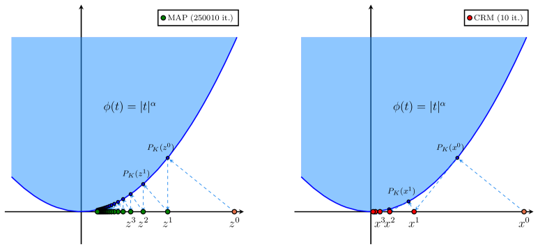
(a) Lack of error bound: MAP converges sublinearly and CRM linearly.

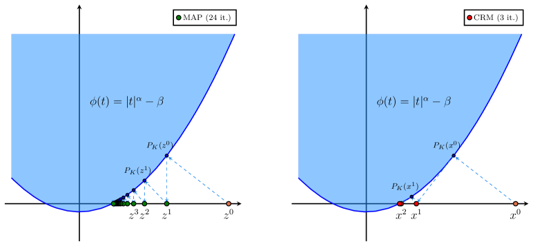
(b) Presence of error bound: MAP converges linearly and CRM superlinearly.

Figure 1: Illustrative comparison between MAP and CRM.

We emphasize that in the cases above MAP exhibits its usual behavior, i.e., linear convergence. The examples of the first family were somewhat special because, roughly speaking, the angle between $K$ and $U$ goes to $0$ near the intersection. On the other hand, the superlinear convergence of CRM is quite remarkable. The additional computations of CRM over MAP reduce to the trivial determination of the reflections and the solution of a system of two linear equations in two variables, for finding the circumcenter Behling:2018a ; Bauschke:2018a . Now MAP is a typical first-order method (projections disregard the curvature of the sets), and thus its convergence is generically no better than linear. We have shown that the CRM acceleration improves this linear convergence to superlinear in a rather large class of instances. Long live CRM!

We conjecture that CRM enjoys superlinear convergence whenever $U$ intersects the interior of $K$. The results in this section firmly support this conjecture.

References

(1)
Aragón Artacho, F.J., Campoy, R., Tam, M.K.: The
Douglas–Rachford algorithm for convex and nonconvex
feasibility problems.
Math Meth Oper Res (2019).
DOI 10.1007/s00186-019-00691-9
(2)
Bauschke, H.H., Bello-Cruz, J.Y., Nghia, T.T.A., Phan, H.M., Wang, X.:
Optimal Rates of Linear Convergence of Relaxed Alternating
Projections and Generalized Douglas-Rachford Methods for Two
Subspaces.
Numer. Algorithms 73(1), 33–76 (2016).
DOI 10.1007/s11075-015-0085-4
(3)
Bauschke, H.H., Borwein, J.M.: On the convergence of von Neumann’s
alternating projection algorithm for two sets.
Set-Valued Analysis 1(2), 185–212 (1993).
DOI 10.1007/BF01027691
(4)
Bauschke, H.H., Borwein, J.M.: On Projection Algorithms for Solving
Convex Feasibility Problems.
SIAM Review 38(3), 367–426 (1996).
DOI 10.1137/S0036144593251710
(5)
Bauschke, H.H., Combettes, P.L.: Convex Analysis and Monotone Operator
Theory in Hilbert Spaces, second edn.
CMS Books in Mathematics. Springer International Publishing
(2017).
DOI 10.1007/978-3-319-48311-5
(6)
Bauschke, H.H., Dao, M.N., Noll, D., Phan, H.M.: Proximal point algorithm,
Douglas-Rachford algorithm and alternating projections: A case study.
J. Convex Anal. 23(1), 237–261 (2016)
(7)
Bauschke, H.H., Ouyang, H., Wang, X.: On circumcenters of finite sets in
Hilbert spaces.
Linear and Nonlinear Analysis 4(2), 271–295 (2018)
(8)
Bauschke, H.H., Ouyang, H., Wang, X.: Circumcentered methods induced by
isometries.
Vietnam Journal of Mathematics 48, 471–508 (2020).
DOI 10.1007/s10013-020-00417-z
(9)
Bauschke, H.H., Ouyang, H., Wang, X.: On the linear convergence of
circumcentered isometry methods.
Numer Algor (2020).
DOI 10.1007/s11075-020-00966-x
(10)
Bauschke, H.H., Ouyang, H., Wang, X.: On circumcenter mappings induced by
nonexpansive operators.
Pure and Applied Functional Analysis in press (2021)
(11)
Behling, R., Bello-Cruz, J.Y., Santos, L.R.: Circumcentering the
Douglas–Rachford method.
Numer Algor 78(3), 759–776 (2018).
DOI 10.1007/s11075-017-0399-5
(12)
Behling, R., Bello-Cruz, J.Y., Santos, L.R.: On the linear convergence of the
circumcentered-reflection method.
Operations Research Letters 46(2), 159–162 (2018).
DOI 10.1016/j.orl.2017.11.018
(13)
Behling, R., Bello-Cruz, J.Y., Santos, L.R.: The block-wise
circumcentered–reflection method.
Comput Optim Appl 76(3), 675–699 (2020).
DOI 10.1007/s10589-019-00155-0
(14)
Behling, R., Bello-Cruz, J.Y., Santos, L.R.: On the
Circumcentered-Reflection Method for the Convex Feasibility
Problem.
Numer. Algorithms (2020).
DOI 10.1007/s11075-020-00941-6
(15)
Behling, R., Fischer, A., Haeser, G., Ramos, A., Schönefeld, K.: On the
constrained error bound condition and the projected
Levenberg–Marquardt method.
Optimization 66(8), 1397–1411 (2017).
DOI 10.1080/02331934.2016.1200578
(16)
Behling, R., Gonçalves, D.S., Santos, S.A.: Local Convergence Analysis
of the Levenberg–Marquardt Framework for
Nonzero-Residue Nonlinear Least-Squares Problems Under an Error
Bound Condition.
J Optim Theory Appl 183(3), 1099–1122 (2019).
DOI 10.1007/s10957-019-01586-9
(17)
Cheney, W., Goldstein, A.A.: Proximity Maps for Convex Sets.
Proceedings of the American Mathematical Society 10(3),
448–450 (1959).
DOI 10.2307/2032864
(18)
Cimmino, G.: Calcolo approssimato per le soluzioni dei sistemi di equazioni
lineari.
La Ricerca Scientifica 9(II), 326–333 (1938)
(20)
Kaczmarz, S.: Angenäherte Auflösung von Systemen linearer
Gleichungen.
Bull. Int. Acad. Pol. Sci. Lett. Class. Sci. Math. Nat. A
35, 355–357 (1937)
(21)
Kayalar, S., Weinert, H.L.: Error bounds for the method of alternating
projections.
Math. Control Signal Systems 1(1), 43–59 (1988).
DOI 10.1007/BF02551235
(22)
von Neumann, J.: Functional Operators, Volume 2: The Geometry of
Orthogonal Spaces.
No. 22 in Annals of Mathematics Studies. Princeton University
Press, Princeton (1950).
DOI 10.2307/j.ctt1bc543b
(23)
Pierra, G.: Decomposition through formalization in a product space.
Mathematical Programming 28(1), 96–115 (1984).
DOI 10.1007/BF02612715