A Multiscale Optimization Framework for Reconstructing Binary Images using Multilevel PCA-based Control Space Reduction

Abstract

An efficient computational approach for optimal reconstructing parameters of binary-type physical properties for models in biomedical applications is developed and validated. The methodology includes gradient-based multiscale optimization with multilevel control space reduction by using principal component analysis (PCA) coupled with dynamical control space upscaling. The reduced dimensional controls are used interchangeably at fine and coarse scales to accumulate the optimization progress and mitigate side effects at both scales. Flexibility is achieved through the proposed procedure for calibrating certain parameters to enhance the performance of the optimization algorithm. Reduced size of control spaces supplied with adjoint-based gradients obtained at both scales facilitate the application of this algorithm to models of higher complexity and also to a broad range of problems in biomedical sciences. This technique is shown to outperform regular gradient-based methods applied to fine scale only in terms of both qualities of binary images and computing time. Performance of the complete computational framework is tested in applications to 2D inverse problems of cancer detection by the electrical impedance tomography (EIT). The results demonstrate the efficient performance of the new method and its high potential for minimizing possibilities for false positive screening and improving the overall quality of the EIT-based procedures.

Keywords: PDE-constrained optimization $\circ$ gradient-based method $\circ$ control space reduction $\circ$ multiscale parameter estimation $\circ$ principal component analysis $\circ$ electrical impedance tomography $\circ$ cancer detection problem

1 Introduction

In this work, we propose and validate a computational approach for optimal reconstructing the physical properties of the media based on any available, possibly incomplete and noisy, measurements. In particular, this approach is useful in various applications in biomedical sciences to operate with physical models characterized by near binary distributions observed for some of their physical properties, e.g. heat or electrical conductivity. The proposed computational framework is using gradient-based multiscale optimization techniques supplied with multilevel control space reduction over both fine and coarse scales used interchangeably. Proper “communication” established between scales in terms of projecting the solution from one scale onto another benefits in both quality and computational efficiency of the obtained results.

As seen in many practical applications, fine scale optimization performed on fine meshes is able to provide high resolution images for the searched distributions. Fine meshes also contribute enormously towards increased sensitivity by enforcing accuracy in computing adjoint states and constructing adjoint-based gradients if in use. The size of the control space defined over fine scales may be significantly decreased by applying any types of parameterization, for instance by using linear transformations based on available sample solutions (realizations) when applying principal component analysis (PCA). However, fine scale optimization may still suffer from over-parameterization if the problem is under-determined, i.e. the number of controls overweighs the size of available data (measurements). On the other hand, optimization performed on coarse meshes could arrive at a solution much faster due to the size of the control space. Usually, the solutions obtained at coarse meshes are of a low quality and less accurate due to sensitivity naturally “coarsened”. In addition to this coarse scale optimization may suffer from being over-determined if the available data and the size of the control space are not properly balanced.

Various techniques of multiscale modeling have been used for decades with proven success for numerous applications in computational mathematics, engineering and computer science. See [32, 40, 23] for a comprehensive description of this general area and an extensive literature review. There is also a recently growing interest in using multiscale techniques in applications to biological and biomedical sciences [5, 38, 15, 34] with limited involvement of methods broadly used in optimization and control theory.

The proposed multiscale optimization framework utilizes all advantages mentioned above while using fine and coarse scales. Moreover, using them both in one process helps us mitigate their side effects. For example, fine scale solution images may not provide clear boundaries between regions identified by different physical properties in space. As a result, a smooth transition cannot provide an accurate recognition of shapes, e.g. of cancer-affected regions while solving an inverse problem of cancer detection (IPCD). In our computations, fine scale optimization is used to approximate the location of regions with high and low values of a physical parameter, namely electrical conductivity. Projecting solutions onto the coarse scale provides a dynamical (sharp-edge) filtering to the fine scale images optimized to better match the available data. The filtered images then projected back onto the fine scale preserving some information on recent changes obtained at the coarse scale. In fact, we developed a computationally efficient procedure for automated scale shifting in order to accumulate optimally progress obtained at both scales. At the extent of how the boundaries of the cancerous spots are recovered by projections between scales with assigned controls at the coarse scale, this approach may be related to a group of level–set methods which utilize multiscale techniques and adaptive grids [30, 18, 35, 12, 28, 26, 33]. We also use some notations, main ideas and governing principles of multiscale parameter estimation (MPE), refer to [19, 20, 16, 26] for some details. In the current paper, we keep the main focus on applying our new computational approach to IPCD by the Electrical Impedance Tomography (EIT) technique, however, the same methodology could be easily applied to a broad range of problems in biomedical sciences, also in physics, geology, chemistry, etc.

EIT is a rapidly developing non-invasive imaging technique gaining popularity by enabling various medical applications to perform screening for cancer detection [41, 9, 3, 22, 36, 27, 1]. A well-known fact is that the electrical properties, e.g. electrical conductivity or permittivity, of different tissues are changing if the status of a tissue is changing from healthy to cancer-affected. This physical phenomenon allows EIT to produce images of biological tissues by interpreting their response to applied voltages or injected currents [9, 13, 22]. A mathematical model for solving different types of EIT problems and performing both analytical and computational analysis of such solutions was suggested in [14]. The inverse EIT problem deals with reconstructing the electrical conductivity by measuring voltages or currents at electrodes placed on the surface of a test volume. This so-called Calderon type inverse problem [11] is highly ill-posed, refer to topical review paper [8]. Since 1980s various computational techniques have been suggested to solve this inverse problem computationally. Recent papers [4, 6, 39] review the current state of the art and the existing open problems associated with EIT and its applications.

This paper proceeds as follows. In Section 2 we present the mathematical description of the inverse EIT as an optimization problem to be solved at both fine and coarse scales by applying control space reduction using PCA (fine scale) and upscaling via dynamical partitioning (coarse scale). Procedures for performing multiscale optimization with interchanging fine and coarse phases are discussed in Section 3. Model descriptions and detailed computational results including optimization parameter calibration are presented in Section 4. Concluding remarks are provided in Section 5.

2 Mathematical Description

2.1 Inverse EIT as an Optimization Problem

In the recent paper [2] the inverse EIT problem is formulated as a PDE-constrained optimization problem in the Besov spaces framework for which the Fréchet gradient and optimality conditions are derived. The authors also developed the projective gradient method in Besov spaces and provided extensive numerical analysis for 2D models by implementing PCA-based solution space re-parameterization and Tikhonov-type regularization. In our current discussion of the inverse EIT model we use the same notations as established in [2].

Let $\Omega\subset\mathbb{R}^{n},\ n=2,3$, be an open and bounded set representing body and we assume that function $\sigma(x):\,\Omega\rightarrow\mathbb{R}_{+}$ represents isotropic electrical conductivity at point $x\in\Omega$. Electrodes $(E_{\ell})_{\ell=1}^{m}$ with contact impedances $(Z_{\ell})_{\ell=1}^{m}\in\mathbb{R}^{m}_{+}$ are attached to the periphery of the body $\partial\Omega$. If the so-called “current–to–voltage” model is used, electrical currents $(I_{\ell})_{\ell=1}^{m}\in\mathbb{R}^{m}$ are applied to the electrodes and induce constant voltages (electrical potentials) $U=(U_{\ell})_{\ell=1}^{m}\in\mathbb{R}^{m}$ on the same electrodes. In this paper, however, we use the “voltage–to–current” model where voltages $U_{\ell}$ are applied to electrodes $E_{\ell}$ to initiate electrical currents $I_{\ell}$. In either model, it is assumed that both electrical currents and voltages satisfy the conservation of charge and ground (zero potential) conditions, respectively

$$\sum_{\ell=1}^{m}I_{\ell}=0,\qquad\sum_{\ell=1}^{m}U_{\ell}=0.$$ (1)

We formulate the inverse EIT (conductivity) problem [11] as a PDE-constrained optimization problem [2] by considering minimization of the following cost functional

$$\mathcal{J}(\sigma)=\sum_{\ell=1}^{m}\left(I_{\ell}-I_{\ell}^{*}\right)^{2},$$ (2)

where $(I_{\ell}^{*})_{\ell=1}^{m}\in\mathbb{R}^{m}$ are measurements made for electrical currents $I_{\ell}$. The latter may be computed as

$$I_{\ell}=\int_{E_{\ell}}\sigma(x)\dfrac{\partial u(x)}{\partial n}\,ds,\quad\ell=1,\ldots,m$$ (3)

based on conductivity field $\sigma(x)$ set here as a control variable. A distribution of electrical potential $u(x):\,\Omega\rightarrow\mathbb{R}$ is obtained as a solution of the elliptic problem

$$\bm{\nabla}\cdot\left[\sigma(x)\bm{\nabla}u(x)\right] =0, \qquad x\in\Omega$$ (4a)

$$\dfrac{\partial u(x)}{\partial n} =0, \qquad x\in\partial\Omega-\bigcup\limits_{\ell=1}^{m}E_{\ell},\ \ell=1,\ldots,m$$ (4b)

$$u(x)+Z_{\ell}\sigma(x)\dfrac{\partial u(x)}{\partial n} =U_{\ell}, \qquad x\in E_{\ell},\ \ell=1,\ldots,m$$ (4c)

in which $n$ is an external unit normal vector on $\partial\Omega$. Here we have to mention a well-known fact that the inverse EIT problem to identify electrical conductivity $\sigma(x)$ in discretized domain $\Omega$ with available input data $(I_{\ell}^{*})_{\ell=1}^{m}$ of size $m$ is highly ill-posed. Therefore, we formulate an optimization problem which is adapted to the situation when the size of input data can be increased through additional measurements while keeping the size of the unknown parameters, i.e. elements in the discretized description for $\sigma(x)$, fixed. Following the discussion in [2] related to the “rotation scheme” we set $U^{1}=U,\ I^{1}=I$ and consider $m-1$ new permutations of boundary voltages

$$U^{j}=(U_{j},\ldots,U_{m},U_{1},\ldots,U_{j-1}),\ j=2,\ldots,m$$ (5)

applied to electrodes $E_{1},E_{2},\ldots,E_{m}$ respectively. Using the “voltage–to–current” model allows us to measure associated currents $I^{j*}=(I^{j*}_{1},\ldots,I^{j*}_{m})$. In addition, the total number of available measurements could be further increased from $m^{2}$ up to $Km^{2}$ by applying (5) to $K$ different permutations of potentials within set $U$. Having a new set of $Km$ input data $(I^{j*})^{Km}_{j=1}$ and in light of the Robin condition (4c) used together with (3), we now consider the optimization problem on minimization of the updated cost functional

$$\mathcal{J}(\sigma)=\sum_{j=1}^{Km}\sum_{\ell=1}^{m}\beta^{j}_{\ell}\left[\int_{E_{\ell}}\dfrac{U^{j}_{\ell}-u^{j}(x;\sigma)}{Z_{\ell}}\,ds-I^{j*}_{\ell}\right]^{2},$$ (6)

where each function $u^{j}(\cdot;\sigma),\ j=1,\ldots,Km$, solves elliptic PDE problem (4a)–(4c). Added weights $\beta^{j}_{\ell}$ in (6) in general allow setting the importance of measurement $I^{j*}_{\ell}$ (when $\beta^{j}_{\ell}>0$), or excluding those measurements ($\beta^{j}_{\ell}=0$) from cost functional $\mathcal{J}$ computations. We also could note that the forward EIT problem (4a)–(4c) together with (3) may be used to generate various model examples (synthetic data) for inverse EIT problems to adequately mimic cancer related diagnoses seen in reality.

Finally, the solution of the optimization problem

$$\hat{\sigma}(x)=\underset{\sigma}{\operatorname{argmin}}\ \mathcal{J}(\sigma)$$ (7)

to minimize cost functional (6) subject to PDE constraint (4) could be obtained by the first-order optimality condition which requires the directional differential of cost functional $\delta\mathcal{J}(\sigma;\delta\sigma)$ to vanish for all perturbations $\delta\sigma$. By invoking the Riesz representation theorem [7] in $L_{2}$ functional space

$$\delta\mathcal{J}(\sigma;\delta\sigma)=\langle\bm{\nabla}_{\sigma}\mathcal{J},\delta\sigma\rangle_{L_{2}}=\int_{\Omega}\bm{\nabla}_{\sigma}\mathcal{J}\,\delta\sigma\,d\Omega,$$ (8)

an iterative algorithm is proposed in [2] to solve problem (7) by means of cost functional adjoint gradients (with respect to control $\sigma$)

$$\bm{\nabla}_{\sigma}\mathcal{J}=-\sum_{j=1}^{Km}\bm{\nabla}\psi^{j}(x)\cdot\bm{\nabla}u^{j}(x)$$ (9)

computed based on solutions $\psi^{j}(\cdot;\sigma):\,\Omega\rightarrow\mathbb{R},\ j=1,\ldots,Km$, of the adjoint PDE problem

$$\bm{\nabla}\cdot\left[\sigma(x)\bm{\nabla}\psi(x)\right] =0, \qquad x\in\Omega$$ (10a)

$$\dfrac{\partial\psi(x)}{\partial n} =0, \qquad x\in\partial\Omega-\bigcup\limits_{\ell=1}^{m}E_{\ell}$$ (10b)

$$\psi(x)+Z_{\ell}\dfrac{\partial\psi(x)}{\partial n} =2\beta_{\ell}\left[\int_{E_{\ell}}\dfrac{u(x)-U_{\ell}}{Z_{\ell}}\,ds+I^{*}_{\ell}\right], \qquad x\in E_{\ell},\ \ell=1,\ldots,m$$ (10c)

2.2 Fine Scale: PCA-based Control Space Reduction

A well-known problem in numerical optimization is that a spatially discretized form of the optimization problem discussed in Section 2.1 is over-parameterized even for small size 2D models. To overcome ill-posedness due to over-parameterization of discretized $\sigma(x)$ along with the fact that the obtained solutions should also honor any available prior information (such as available images, etc.), we implement re-parameterization of the control space based on principal component analysis, also known as Proper Orthogonal Decomposition (POD) or Karhunen–Loève (KL) expansion.

More specifically, PCA enables us to represent control $\sigma(x)$ in terms of uncorrelated variables (components of vector $\xi$) mapping $\sigma(x)$ and $\xi$ by

$$\sigma =\Phi\,\xi+\bar{\sigma},$$ (11a)

$$\xi =\hat{\Phi}^{-1}(\sigma-\bar{\sigma}),$$ (11b)

where $\Phi$ is the basis (linear transformation) matrix, $\hat{\Phi}^{-1}$ is the pseudo-inverse of $\Phi$, and $\bar{\sigma}$ is the prior mean. In the PCA used in our numerical experiments, the truncated singular value decomposition (TSVD) of a (centered) matrix, containing $N_{r}$ sample solutions (realizations) $(\sigma^{*}_{n})_{n=1}^{N_{r}}$, as its columns, is used to construct the basis matrix $\Phi$. The prior mean is given by $\bar{\sigma}=(1/N_{r})\sum_{n=1}^{N_{r}}\sigma^{*}_{n}$, see [2, 10, 25, 24] for PCA theory in general and details on constructing a complete PCA representation in particular. The optimization problem initially defined in Section 2.1 is now restated in terms of new model parameters $\xi\in\mathbb{R}^{N_{\xi}}$ used in place of control $\sigma(x)$ as follows

$$\hat{\xi}=\underset{\xi}{\operatorname{argmin}}\ \mathcal{J}(\xi)$$ (12)

subject to discretized PDE model (4) and using control mapping (11) for computing $\mathcal{J}(\xi)=\mathcal{J}(\sigma(\xi))$. New gradients $\bm{\nabla}_{\xi}\mathcal{J}$ of cost functional $\mathcal{J}(\sigma)$ with respect to new control $\xi$ can be expressed as

$$\bm{\nabla}_{\xi}\mathcal{J}=\Phi^{T}\,\bm{\nabla}_{\sigma}\mathcal{J}$$ (13)

to define projection of gradients $\bm{\nabla}_{\sigma}\mathcal{J}$ obtained by (9) from initial (physical) $\sigma$-space onto the reduced-dimensional $\xi$-space.

2.3 Coarse Scale: Control Space Upscaling via Partitioning

An optimum in employing PCA-based control space reduction on a fine mesh discussed in Section 2.2 will be achieved by finding the minimal (optimal) size of new control $\xi$ to enable honoring prior information from available sample solutions [2, 10]. As often seen in practical applications, this optimal size cannot prevent the optimization problem (12) from being still over-parameterized. Therefore, one will be interested in further re-parameterization by finding a new control space defined by a reasonably small number of parameters, and thus, having fewer local minima.

As a motivation for our new multiscale approach we used an idea of gradient-based multiscale (parameter) estimation (GBME) raised from the general MPE principles [16]. Figure 1 illustrates the general concept of GBME. It employs various approaches for gradient-based refinement of the control space for dynamical space upscaling, i.e. control grouping, by analysis of changes in the gradient structure. For example, “noncompetitive” controls identified by relatively small components in the gradient, shown in red in Figures 1(a,b), are grouped into a new control. The associated (cumulative) component of the upscaled gradient, added as a red bar in Figure 1(c), makes the new control competitive and “visible” by other controls shown in blue and green.

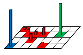
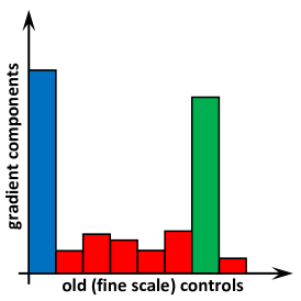
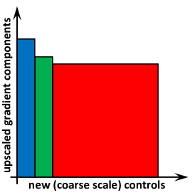
Figure 1: Schematic illustrating the general concept of gradient-based multiscale estimation (GBME). Plots in (a,b) show “noncompetitive” vs. “competitive” controls identified by associated small (red bars) and big (blue and green bars) components of the gradient. A new (cumulative) gradient component obtained via control grouping is depicted by the big red bar in (c) with dimensions compounded by summing the respective dimensions of small red bars in (b). For simplicity, all gradients shown in (a,b,c) have only positive components.

Keeping aside for a while a principle by which spatial controls are grouped (partitioned) in our new approach, let us focus on obtaining upscaled gradients for new controls $(\zeta_{j})_{j=1}^{N_{\zeta}}\in\mathbb{R}^{N_{\zeta}}_{+}$. We assume that control $\sigma(x)$ in problem (7) is discretized over the fine mesh containing $N$ elements and represented by a finite set of controls $(\sigma_{i})_{i=1}^{N}\in\mathbb{R}^{N}_{+}$. This set is then partitioned into $N_{\zeta}$ subsets $C_{j},\ j=1,\ldots,N_{\zeta}$, by selecting (without repetition) $N_{j}$ controls for $j$-th subset and defining a map, i.e. fine–to-coarse partition,

$$\mathcal{M}:\,(\sigma_{i})_{i=1}^{N}\rightarrow\bigcup\limits_{j=1}^{N_{\zeta}}C_{j},\quad C_{j}=\{\sigma_{i}:P_{i,j}=1,\,i=1,\ldots,N\},\quad\sum_{j=1}^{N_{\zeta}}|C_{j}|=\sum_{j=1}^{N_{\zeta}}N_{j}=N,$$ (14)

where the partition indicator function is defined as

$$P_{i,j}=\left\{\begin{aligned} 1,\quad\sigma_{i}\in C_{j},\\ 0,\quad\sigma_{i}\notin C_{j}.\end{aligned}\right.$$ (15)

To proceed with gradients, we now consider discretized directional differential $\delta\tilde{\mathcal{J}}$, obtained from (8) by the first-order scheme, which is consistent with the discretized form of domain $\Omega$ decomposed into $N$ spatial elements $(\delta\Omega_{i})_{i=1}^{N}$ each of area (or volume in 3D) $\Delta_{i}$

$$\delta\mathcal{J}(\sigma;\delta\sigma)\approx\delta\tilde{\mathcal{J}}=\sum_{i=1}^{N}\dfrac{\partial\mathcal{J}}{\partial\sigma_{i}}\Delta_{i}\,\delta\sigma_{i},$$ (16)

where $\delta\sigma_{i}$ perturbs controls $\sigma_{i}$. Whenever control grouping is in place, we assume that all controls $\sigma_{i}$ within the same $j$-th group, $\sigma_{i}\in C_{j}$, are perturbed equally, i.e. $\delta\sigma_{i}=\delta\zeta_{j}$ if $P_{i,j}=1$ for all $i=1,\ldots N$ and $j=1,\ldots N_{\zeta}$. Then one could easily show that the spatial grouping is fully consistent with the Riesz theorem

$$\delta\tilde{\mathcal{J}}=\sum_{j=1}^{N_{\zeta}}\sum_{i=1}^{N}P_{i,j}\dfrac{\partial\mathcal{J}}{\partial\sigma_{i}}\Delta_{i}\,\delta\sigma_{i}=\sum_{j=1}^{N_{\zeta}}\dfrac{\partial\mathcal{J}}{\partial\zeta_{j}}\,\delta\zeta_{j}=\langle\bm{\nabla}_{\zeta}\mathcal{J},\delta\zeta\rangle$$ (17)

and upscaled gradients $\bm{\nabla}_{\zeta}\mathcal{J}$ are computed by summing up those components of discretized gradients $\bm{\nabla}_{\sigma}\mathcal{J}$ related to controls $\sigma_{i}\in C_{j}$, i.e.

$$\dfrac{\partial\mathcal{J}}{\partial\zeta_{j}}=\sum_{i=1}^{N}P_{i,j}\dfrac{\partial\mathcal{J}}{\partial\sigma_{i}}\Delta_{i}.$$ (18)

In general, a gradient-based framework to perform optimization on multiple, fine and coarse, meshes will benefit from the following.

• Forward simulations on fine N-element meshes allow constructing highly accurate adjoint-based gradients $\bm{\nabla}_{\sigma}\mathcal{J}$.

• Reasonably small number of controls $N_{\zeta}\ll N$ defined at coarse scales tends to lessen the number of local minima.

• Upscaling gradients at coarse scales by (18) allows dynamical control space relaxation without interrupting iterative optimization to follow changes in upscaling map (14).

Figure 2 illustrates the general concept of such dynamical control space relaxation and obtaining upscaled gradients for two new controls at a coarse scale. As shown in Figures 2(a,b), gradient components for all fine mesh controls may have the same order of magnitude. Thus, these controls, shown in red and blue, could be grouped following the idea which is different from the analysis of the gradient structure used in GBME. We discuss this in detail as a new grouping (partitioning) approach in Section 3.3.

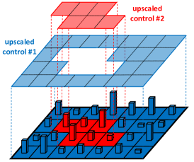
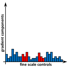
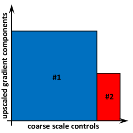
Figure 2: Schematic illustrating the general concept of dynamical control space relaxation and obtaining upscaled gradients at coarse scale by making 2-group assignments for fine scale controls, $N_{\zeta}=2$. Plots in (a,b) show all controls on a fine mesh. Different colors are used to identify controls to be included into (blue) upscaled control #1 and (red) upscaled control #2. The new (cumulative) gradient components obtained via control grouping (partitioning) are depicted by the big blue and red bars in (c) with dimensions compounded by summing the respective dimensions of small blue and red bars in (b). For simplicity, all gradients shown in (a,b,c) have only positive components.

3 Multiscale Optimization Framework

3.1 Switching Between Scales

The proposed approach for optimization utilizing multilevel control space reduction over multiple scales, both fine and coarse, is motivated by a range of possible applications in biomedical sciences. These applications are based on physical models represented by binary distributions of some physical properties, e.g. electrical conductivity $\sigma(x)$ in EIT. Figure 3(left) shows an example of the histogram typical for such distributions.

A common approach to solve optimization problem (7) is to solve problem (12) instead by applying PCA-based space reduction by mapping $N$-element (fine-mesh) $\sigma$-space and reduced-dimensional $\xi$-space. An optimal solution $\hat{\sigma}(x)$ obtained after applying map (11a) to $\hat{\xi}$ is of a Gaussian type. In case one of two modes is relatively small, a histogram for the solution image is hardly recognized as being bimodal, e.g. as shown in Figure 3(middle), and possible conversions to binary images may be very inaccurate.

To provide a remedy and obtain the optimal solution $\hat{\sigma}(x)$ of a required binary type the proposed approach employs multiscale optimization at both fine and coarse scales each with their own sets of controls by using them interchangeably. While various schemes are available for switching between scales, here we consider a simple one: scales are changed every $n_{s}$ optimization iterations. We also define the coarse scale indicator function

$$\chi_{c}(k)=\left\{\begin{aligned} 0,\quad(2k_{s}-2)n_{s}&<k\leq(2k_{s}-1)n_{s},&&\quad{\rm(fine\ scale)}\\ 1,\quad(2k_{s}-1)n_{s}&<k\leq 2k_{s}n_{s},&&\quad{\rm(coarse\ scale)}\end{aligned}\right.$$ (19)

where $k_{s}=1,2,\ldots$ and $k=0,1,2,\ldots$ denote respectively the counts for switching cycles and optimization iterations. We choose to terminate the optimization run once the following criterion is satisfied

$$\left|\dfrac{\mathcal{J}(\sigma^{k})-\mathcal{J}(\sigma^{k-1})}{\mathcal{J}(\sigma^{k})}\right|<(1-\chi_{c})\epsilon_{f}+\chi_{c}\epsilon_{c},\quad k\neq k_{s}n_{s}+1$$ (20)

subject to chosen tolerances $\epsilon_{f},\epsilon_{c}\in\mathbb{R}_{+}$.

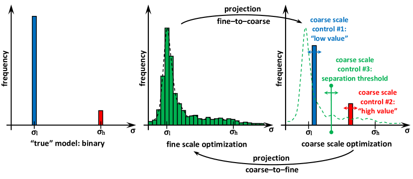
Figure 3: Schematic illustrating the general concept of the multiscale optimization framework. (left) A typical histogram representing binary distribution of true electrical conductivity $\sigma(x)$ used in EIT. In all three plots $\sigma_{l}$ and $\sigma_{h}$ values represent two modes associated respectively with healthy and cancer-affected regions within domain $\Omega$. (middle) An example of the Gaussian-type histogram typical for solution $\sigma^{k}(x)$ obtained after $k$ iterations at a fine scale. (right) A binary histogram for solution $\sigma^{k}(x)$ obtained at $k$-th iteration at a coarse scale. Positions of blue and red bars are associated with current values of $\sigma^{k}_{low}$ and $\sigma^{k}_{high}$ controls, while their heights are computed based on the fine scale representation $\sigma(\xi^{k})$ cut off by the current value of the coarse scale threshold control $\sigma^{k}_{th}$. See Sections 3.2–3.3 for details. Coarse–to–fine and fine–to–coarse projections are defined respectively by (21)–(23) and (25)–(29).

Our multiscale optimization framework is shown schematically in Figures 3(middle,right). Here, we would like to emphasize that all solutions obtained at both fine and coarse scales are represented on (projected onto) the same $N$-element fine mesh. The word “multiscale”, in fact, refers to updates provided to discretized control $\sigma(x)$. At a fine scale all elements $\sigma_{i},\,i=1,\ldots,N$, are updated by applying PCA-based transformation, while at a coarse scale these elements are sorted into two groups and then updated within each group by following the same rule. We discuss optimization phases at both scales as well as switching procedures in the following two sections.

3.2 Fine Scale Phase

We denote the solution for control $\sigma^{k}=\sigma^{k}(x)$ obtained at a fine scale at $k$-th iteration as $\sigma(\xi^{k})$. During the fine scale optimization phase, $\chi_{c}(k)=0$, control $\sigma^{k}$ is updated by solving optimization problem (12) in the reduced-dimensional $\xi$-space and by using map (11a) as described in Section 2.2, i.e. $\sigma^{k}=\sigma(\xi^{k})$. Alternatively, during the coarse scale optimization phase ($\chi_{c}(k)=1$) $\sigma(\xi^{k})$, updated last time at the end of the fine scale phase, is used in coarse scale control grouping discussed in Section 3.3.

To start the first switching cycle, $k_{s}=1$, and optimization itself, $k=0$, the initial guess $\sigma^{0}$ may be taken, for instance, corresponding to any approximate theoretical prediction $\sigma_{0}(x)$. It is obvious that every time when coarse scale switches to the fine one, $k=2k_{s}n_{s},\,k_{s}\geq 1$, fine scale controls $\xi^{k}$ should be updated to ensure it receives as much as possible information related to recent changes in $\sigma^{k}$ during the coarse scale phase. On the other hand, this update should not worsen the results $\sigma(\xi^{k})$ previously obtained at the fine scale. Here, we propose the following scheme to project solution $\sigma^{k}$ obtained at the end of the coarse scale phase onto $\xi$-space by using a convex combination of $\sigma(\xi^{k})$ and $\sigma^{k}$

$$\forall k=2k_{s}n_{s},\,k_{s}\geq 1:\ \ \bar{\sigma}(\xi^{k})=\alpha_{c\rightarrow f}\,\sigma(\xi^{k})+(1-\alpha_{c\rightarrow f})\,\sigma^{k},\quad\alpha_{c\rightarrow f}\in[0,1].$$ (21)

Control $\xi^{k}$ then could be re-initialized from $\bar{\sigma}(\xi^{k})$ by using map (11b). As $\bar{\sigma}(\xi^{k})$ and $\sigma^{k}$ have different distributions, namely of Gaussian and binary types, the coarse–to–fine projection scheme (21) may benefit from projecting $\sigma^{k}$ first to its PCA equivalent

$$\sigma^{k}_{PCA}=\Phi\hat{\Phi}^{-1}(\sigma^{k}-\bar{\sigma})+\bar{\sigma},$$ (22)

see [37, 10] for details. $\sigma^{k}_{PCA}$ then could be used in (21) in place of $\sigma^{k}$. Also, an optimal choice of relaxation parameter $\alpha_{c\rightarrow f}$ could be made by solving the following optimization problem in 1D

$$\alpha_{c\rightarrow f}=\hat{\alpha}=\underset{\begin{array}[]{cc}0\leq\alpha\leq 1\\ \mathcal{J}(\bar{\sigma}(\xi^{k}))\leq\mathcal{J}(\sigma(\xi^{k}))\end{array}}{\operatorname{argmin}\ \alpha}$$ (23)

which appears to be highly nonlinear due to the inequality constraint to control the quality of fine scale solutions $\sigma(\xi^{k})$ in transition between subsequent switching cycles.

3.3 Coarse Scale Phase

To run optimization at a coarse scale we define a new 3-component control vector $\zeta=(\zeta_{j})_{j=1}^{3}$ in which the first two entries are the low and high values of (binary) electrical conductivity $\sigma(x)$ associated with healthy and cancer-affected regions in domain $\Omega$, i.e.

$$\zeta_{1}=\sigma_{low},\quad\zeta_{2}=\sigma_{high}.$$ (24)

They are shown schematically as respectively blue and red bars in Figure 3(right). The third component, $\zeta_{3}=\sigma_{th}$, takes responsibility for the shape of those regions (healthy and cancer-affected) and is set as a separation threshold to define a boundary between low and high conductivity regions as shown in green in Figure 3(right). Such a simple structure of control $\zeta$ allows us to create a simplified representation of the coarse scale solution $\zeta^{k}$ for control $\sigma^{k}$ at $k$-th iteration based on the current fine scale representation $\sigma(\xi^{k})=(\sigma_{i}(\xi^{k}))_{i=1}^{N}$

$$\sigma^{k}_{i}=\left\{\begin{aligned} \sigma^{k}_{low},&\quad\sigma_{i}(\xi^{k})<\sigma^{k}_{th},\\ \sigma^{k}_{high},&\quad\sigma_{i}(\xi^{k})\geq\sigma^{k}_{th},\end{aligned}\right.\qquad i=1,\ldots N,$$ (25)

where

$$0<\sigma^{k}_{low}<\sigma^{k}_{high},\qquad\underset{i}{\min}\ \sigma_{i}(\xi^{k})<\sigma^{k}_{th}<\underset{i}{\max}\ \sigma_{i}(\xi^{k}),\ i=1,\ldots N.$$ (26)

Simply, (25) provides a rule for creating fine–to–coarse partition $\mathcal{M}$ in (14) when $N_{\zeta}=2$ based on the current state of control $\zeta$. During the coarse scale optimization phase, $\chi_{c}(k)=1$, control $\sigma^{k}$ is updated by solving a 3D optimization problem in the $\zeta$-space

$$\hat{\zeta}=\underset{\zeta}{\operatorname{argmin}}\ \mathcal{J}(\zeta)$$ (27)

subject to constraints (bounds) provided in (26), and then $\sigma^{k}=\sigma(\zeta^{k})$. When solving problem (27) during the first switching cycle, $k=n_{s}$, $\zeta^{k}$ could be initially approximated by some constants, for example

$$\sigma^{k}_{th} =\frac{1}{2}\left[\underset{i}{\max}\ \sigma_{i}(\xi^{k})+\underset{i}{\min}\ \sigma_{i}(\xi^{k})\right],$$ (28)

$$\sigma^{k}_{low} =\underset{i}{\operatorname{mean}}\left\{\sigma_{i}(\xi^{k}):\ \sigma_{i}(\xi^{k})<\sigma^{k}_{th}\right\},$$

$$\sigma^{k}_{high} =\underset{i}{\operatorname{mean}}\left\{\sigma_{i}(\xi^{k}):\ \sigma_{i}(\xi^{k})\geq\sigma^{k}_{th}\right\},\quad i=1,\ldots N.$$

Switching from fine scale to coarse one when $k=(2k_{s}-1)n_{s},\ k_{s}>1$, could be even more straightforward by utilizing the components of control $\zeta$ obtained at the previous coarse scale phase, i.e.

$$\zeta^{k}=\zeta^{k-2n_{s}}.$$ (29)

In order to solve (27) by any approach which requires computing a gradient, its first two components

$$\dfrac{\partial\mathcal{J}(\zeta)}{\partial\zeta_{1}}=\dfrac{\partial\mathcal{J}}{\partial\sigma_{low}},\quad\dfrac{\partial\mathcal{J}(\zeta)}{\partial\zeta_{2}}=\dfrac{\partial\mathcal{J}}{\partial\sigma_{high}}$$

could be easily obtained by using gradient summation formula (18) after completing partitioning map $\mathcal{M}$ (14)–(15) by employing (25). On the other hand, the third component may be approximated by a finite difference scheme, e.g. of the first order,

$$\dfrac{\partial\mathcal{J}(\zeta)}{\partial\zeta_{3}}=\dfrac{\partial\mathcal{J}}{\partial\sigma_{th}}=\dfrac{\mathcal{J}\left(\sigma^{k}(\zeta_{1},\zeta_{2},\zeta_{3}+\delta_{\zeta})\right)-\mathcal{J}\left(\sigma^{k}(\zeta_{1},\zeta_{2},\zeta_{3})\right)}{\delta_{\zeta}}+\mathcal{O}(\delta_{\zeta}).$$ (30)

Parameter $\delta_{\zeta}$ in (30) is to be set experimentally pursuing trade-off between being reasonably small to ensure accuracy and large enough to protect numerator from being zero. In fact, formulas (25)–(29) provide a complete description of the fine–to–coarse projection for control $\sigma(x)$ used in our approach. A summary of the complete computational scheme to perform our new PCA-based multilevel optimization over multiple scales is provided in Algorithm 1.

  $k\leftarrow 0$

  $\chi_{c}\leftarrow 0$

  $\sigma^{0}\leftarrow$ initial guess $\sigma_{0}(x)$

  compute $\xi^{0}$ using $\sigma^{0}$ by (11b)

  repeat

     compute $u^{k}$ using $\sigma^{k}$ by solving forward problem (4)

     compute $\psi^{k}$ using $u^{k}$ and $\sigma^{k}$ by solving adjoint problem (10)

     compute $\bm{\nabla}_{\sigma}\mathcal{J}(\sigma^{k})$ using $u^{k}$ and $\psi^{k}$ by (9)

     if $\chi_{c}=1$ then

        compute $\sigma(\xi^{k})$ using $\xi_{k}$ by (11a)

        compute $\bm{\nabla}_{\zeta}\mathcal{J}(\zeta^{k})$ using $\zeta^{k},\sigma(\xi^{k}),$ and $\bm{\nabla}_{\sigma}\mathcal{J}(\sigma^{k})$ by (18), (14)–(15), (25), and (30)

     else

        compute $\bm{\nabla}_{\xi}\mathcal{J}(\xi^{k})$ using $\bm{\nabla}_{\sigma}\mathcal{J}(\sigma^{k})$ by (13)

     end if

     update $\zeta^{k+1}$ and $\xi^{k+1}$ by using, depending on $\chi_{c}(k)$, descent directions $D_{\zeta}\left(\bm{\nabla}_{\zeta}\mathcal{J}\right)$ or $D_{\xi}\left(\bm{\nabla}_{\xi}\mathcal{J}\right)$ obtained respectively from $\bm{\nabla}_{\zeta}\mathcal{J}(\zeta^{k})$ or $\bm{\nabla}_{\xi}\mathcal{J}(\xi^{k})$

$$\zeta^{k+1} =\zeta^{k}-\chi_{c}(k)\tau^{k}D_{\zeta}\left(\bm{\nabla}_{\zeta}\mathcal{J}(\zeta^{k})\right),$$ (31a)

$$\xi^{k+1} =\xi^{k}-(1-\chi_{c}(k))\tau^{k}D_{\xi}\left(\bm{\nabla}_{\xi}\mathcal{J}(\xi^{k})\right)$$ (31b)

     if $\chi_{c}=1$ then

        compute $\sigma^{k+1}$ using $\zeta^{k+1}$ and $\sigma(\xi^{k+1})$ by (25)

     else

        compute $\sigma^{k+1}$ using $\xi^{k+1}$ by (11a)

     end if

     $k\leftarrow k+1$

     update $\chi_{c}$ using $k$ by (19)

     if $\chi_{c}(k)\neq\chi_{c}(k-1)$ then

        if $\chi_{c}=1$ then

           update $\sigma^{k}$ using $\zeta^{k}$ and $\sigma(\xi^{k})$ by (25)

        else

           update $\xi^{k}$ using $\sigma^{k}$ and $\sigma(\xi^{k})$ by (21)–(23)

           update $\sigma^{k}$ using $\xi^{k}$ by (11a)

        end if

     end if

  until termination criterion (20) is satisfied to given tolerances $\epsilon_{f}$ and $\epsilon_{c}$

Algorithm 1 Computational workflow for PCA-based multiscale optimization

4 Main Results

4.1 Computational Model in 2D

Our optimization framework integrates computational facilities for solving forward PDE problem (4), adjoint PDE problem (10), and evaluation of the gradients according to (9), (13), and (18). These facilities are incorporated mainly by using FreeFem++, see [21] for details, an open–source, high–level integrated development environment for obtaining numerical solutions of PDEs based on the Finite Element Method (FEM). For solving numerically forward PDE problem (4), spatial discretization is carried out by implementing FEM triangular finite elements: P2 piecewise quadratic (continuous) representation for electrical potential $u(x)$ and P0 piecewise constant representation for conductivity field $\sigma(x)$. Systems of algebraic equations obtained after such discretization are solved with UMFPACK, a solver for nonsymmetric sparse linear systems [17]. The same technique is used for numerical solutions of adjoint problem (10). All computations are performed using 2D domain

$$\Omega=\left\{x\in\mathbb{R}^{2}:\ x_{1}^{2}+x_{2}^{2}<r^{2}_{\Omega}\right\}$$ (32)

which is a disc of radius $r_{\Omega}=0.1$ with $m=16$ equidistant electrodes $E_{\ell}$ with half-width $w=0.12$ rad covering approximately 61% of boundary $\partial\Omega$ as shown in Figure 4(a). Electrical potentials $U_{\ell}$, see Figure 4(b), are applied to electrodes $E_{\ell}$ as seen in (5) following the “rotation scheme” discussed in Section 2.1. We also consider adding up to three additional permutations within the set of potentials $U$, and, by choosing $K\in\left\{1,2,3,4\right\}$, we increase the total number of measurements from $m^{2}=256$ ($K=1$) to $Km^{2}=1024$ ($K=K_{\max}=4$). The potentials are chosen to be consistent with the ground potential condition (1). Determining the Robin part of the boundary conditions in (4c) we equally set the electrode contact impedance $Z_{\ell}=0.1$. Figure 4(c) also shows an example of the distribution of flux $\sigma(x)\bm{\nabla}u(x)$ of electrical potential $u(x)$ in the interior of domain $\Omega$ during EIT.

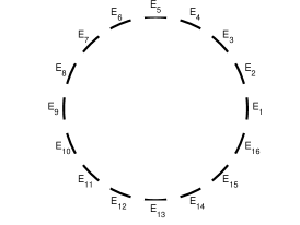
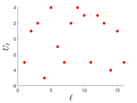
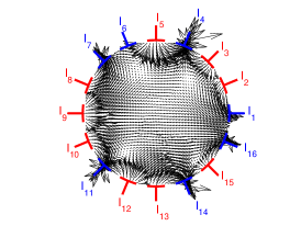
Figure 4: (a) Equispaced geometry of electrodes $E_{\ell},\ \ell=1,2,\ldots,16$, placed over boundary $\partial\Omega$. (b) Electrical potentials $U_{\ell}$. (c) Electrical currents $I_{\ell}$ (positive in red, negative in blue) measured at electrodes $E_{\ell}$. Black arrows show the distribution of flux $\sigma(x)\bm{\nabla}u(x)$ of electrical potential $u(x)$ in the interior of domain $\Omega$.

Physical domain $\Omega$ is discretized using mesh created by specifying $176$ vertices over boundary $\partial\Omega$ and totaling $N=7726$ triangular FEM elements inside $\Omega$. This fine mesh is then used to construct gradients $\bm{\nabla}_{\sigma}\mathcal{J}$, $\bm{\nabla}_{\xi}\mathcal{J}$, and $\bm{\nabla}_{\zeta}\mathcal{J}$ to perform the optimization procedure as described in Algorithm 1. To solve problems (27) and (12) iteratively as seen in (31), our framework is utilizing respectively the Steepest Descent (SD) and Conjugate Gradient (CG) approaches [29] to obtain descent directions $D_{\zeta}$ and $D_{\xi}$. Stepsize parameters $\tau^{k}$ in (31) are obtained by applying line minimization search [31].

The actual (true) electrical conductivity $\sigma_{true}(x)$ we seek to reconstruct will be given analytically for each model by

$$\sigma_{true}(x)=\left\{\begin{aligned} \sigma_{c},&\quad x\in\Omega_{c},\\ \sigma_{h},&\quad x\in\Omega_{h},\end{aligned}\right.\qquad\Omega=\Omega_{c}\cup\Omega_{h},\qquad\Omega_{c}\cap\Omega_{h}=\emptyset$$ (33)

and setting $\sigma_{c}=0.4$ for cancer-affected region $\Omega_{c}$ (up to 4 spots of different size depending on the model’s complexity) and $\sigma_{h}=0.2$ to healthy tissues part $\Omega_{h}$. In terms of the initial guess for control $\sigma(x)$ we take a constant approximation to $\sigma_{true}$ given by $\sigma_{0}=\frac{1}{2}\left(\sigma_{h}+\sigma_{c}\right)=0.3$. In order to avoid early termination at a coarse scale, termination tolerances in (20) are set as $\epsilon_{c}=0$ and $\epsilon_{f}=10^{-10}$.

To simplify the enforcement of bounds established for coarse scale control $\sigma^{k}_{th}$ in (26), in all computations we used fine–to–coarse partition (25) redefined as

$$\sigma^{k}_{i}=\left\{\begin{aligned} \sigma^{k}_{low},&\quad\sigma_{i}(\xi^{k})<(1-\sigma^{k}_{th})\,\underset{i}{\min}\ \sigma_{i}(\xi^{k})+\sigma^{k}_{th}\,\underset{i}{\max}\ \sigma_{i}(\xi^{k}),\\ \sigma^{k}_{high},&\quad{\rm otherwise},\end{aligned}\right.\qquad i=1,\ldots N,$$ (34)

while ensuring $0<\sigma^{k}_{th}<1$.

For all computations mentioned in the rest of Section 4 we use a PCA-based map (11) between $N$-dimensional discretized control $\sigma(x)$ and reduced-dimensional $\xi$-space as described in Section 2.2. A set of $N_{r}=1000$ realizations $(\sigma^{*}_{n})_{n=1}^{1000}$ is created using a generator of uniformly distributed random numbers. Each realization $\sigma^{*}_{n}$ “contains” from one to seven “cancer-affected” areas with $\sigma_{c}=0.4$. Each area is located randomly within domain $\Omega$ and represented by a circle of randomly chosen radius $0<r\leq 0.3r_{\Omega}$. To perform TSVD we choose the number of principal components $N_{\xi}$ by retaining 662, 900, and 965 basis vectors in the PCA description. These values correspond to the preservation of respectively $r_{\xi}=99\%$, $99.9\%$, and $99.99\%$ of the “energy” in the full set of basis vectors, see [2, 10] for details.

4.2 Parameter Calibration

We created our (benchmark) model #1 to check the performance of the proposed optimization framework and discuss the procedure for calibrating its certain parameters. This model in fact mimics a simple situation when a biological tissue contains one circular-shaped area suspicious to be affected by cancer as seen in Figures 5(a,b).

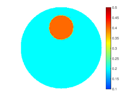
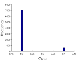
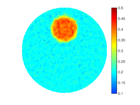
Figure 5: Model #1. (a) True electrical conductivity $\sigma_{true}(x)$. (b) A binary-type histogram for model #1. (c) Electrical conductivity $\sigma_{PCA}(x)$ for model #1 obtained by projecting $\sigma_{true}(x)$ to its PCA equivalent with $r_{\xi}=99\%$ by using (22).

Here, we would like to address a well-known issue on the presence of noise in measurements due to improper electrode–tissue contacts, wire interference, possible electrode misplacement, etc. Its negative impact has been already investigated by many researchers both theoretically and within practical applications. Although all results in this paper are obtained without explicit noise added to measurements, our synthetic data features effects similar to those when noise is present. First, “measured” electrical currents $I^{*}_{\ell}$ are recorded by running (4) and (3) with $\sigma(x)=\sigma_{true}$ represented by P2 FEM elements. Then, as mentioned in Section 4.1, the actual reconstruction $\hat{\sigma}(x)$ is obtained in P0 finite element space. Taking also into account that the “measurement” data is not projected into its PCA equivalent, we compared cost functional $\mathcal{J}(\sigma)$ evaluated at $\sigma_{true}$ with added noise and at $\sigma_{PCA}$, as shown in Figure 5(c), obtained after applying PCA projection. The equivalent noise is estimated to be at level $0.2\%-0.3\%$.

In order to evaluate the performance, we define a set $\mathcal{S}=\left\{K,\ r_{\xi},\ j_{\max},\ n_{s}\right\}$ of 4 major parameters to be calibrated:

• $K\in\{1,2,3,4\}$ to define the total number of measurements, $Km^{2}$, respectively as 256, 512, 768, 1024,

• $r_{\xi}\in\{99\%,99.9\%,99.99\%\}$ to set the number of principal components, i.e. number of controls $N_{\xi}$ at a fine scale, respectively to 662, 900, 965,

• $j_{\max}\in\{1,Km\}$ to consider two cases for optimization at the coarse scale: $\beta^{j}_{\ell}=1,\,j=1,\ldots,Km$, vs. $\beta^{j}_{\ell}=0$ except $j=1$ to consider respectively full data vs. $m=16$ measurements to avoid over-parameterization, and

• $n_{s}\in\{5,10\}$ frequency of switching between fine and coarse scales.

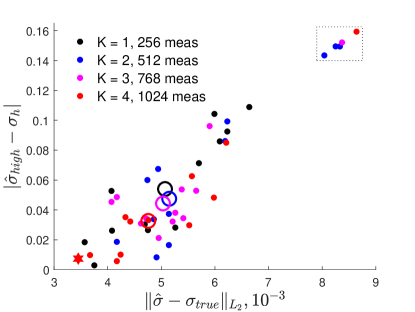
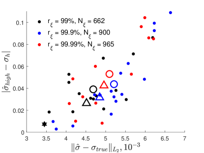
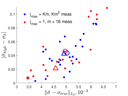
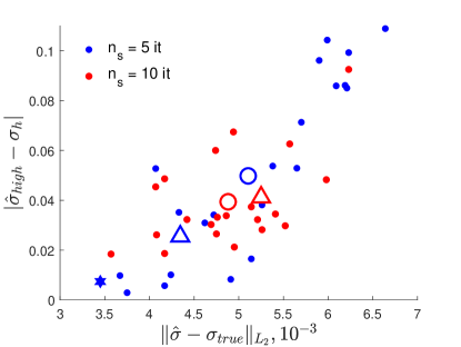
Figure 6: Model #1 calibration results. Different colors are used for different values of parameters (a) $K=1,2,3,4$, (b) $r_{\xi}=99\%,99.9\%,99.99\%$, (c) $j_{\max}=1,Km$, and (d) $n_{s}=5,10$. Open circles in (a) provide the results averaged over four cases $K=1,2,3,4$. Open circles and triangles in (b,c,d) represent averages obtained respectively for $K=1$ and $K=4$. Five outliers shown inside the dotted box in (a) are removed from plots in (b,c,d). The result obtained with parameter schedule $\mathcal{S}^{*}$ in (35) is shown by stars in all four plots.

Figure 6 shows the results obtained after performing the calibration procedure, i.e. after running optimization for model #1 with 48 different parameter schedules $\mathcal{S}$. We have chosen two critical factors to evaluate the performance in each case: the $L_{2}$-norm difference between optimal solution $\hat{\sigma}(x)$ and true conductivity field $\sigma_{true}(x)$ ($x$-axis), and the absolute error in recovered $\hat{\sigma}_{high}$ by comparing it with the known value $\sigma_{h}=0.4$ ($y$-axis). We note that for all experiments $\hat{\sigma}_{low}$ is recovered very accurately. Five outliers inside the dotted box in Figure 6(a) are excluded from the entire calibration statistics. Then open circles in Figure 6(a) provide the results averaged over four cases, $K=1,2,3,4$, with $K=4$ (red circle) appeared as the best one. Figures 6(b,c,d) show the same $43$ outcomes (less 5 outliers) then colored according to values of the rest parameters, namely $r_{\xi},j_{\max}$, and $n_{s}$. Open circles and triangles there represent averages obtained respectively for $K=1$ and $K=4$. We conclude that simple models, like our model #1, will be best reconstructed with 99% PCA, limited data at a coarse scale, and by switching between scales every 5 iterations, i.e. our calibration returns the following schedule

$$\mathcal{S}^{*}=\left\{K=4,\ r_{\xi}=99\%,\ j_{\max}=1,\ n_{s}=5\right\}.$$ (35)

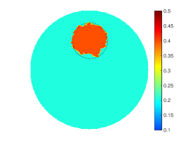
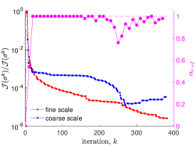
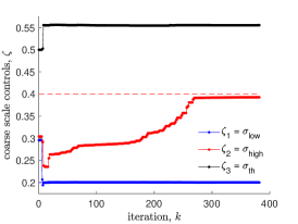
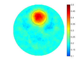
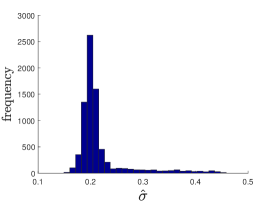
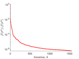
Figure 7: Model #1 optimization outcomes: (a,b,c) after applying the multiscale framework by Algorithm 1, and (d,e,f) when optimization is performed only at a fine scale. Plots in (a,d) show the obtained images with added dotted circles to represent the location of the cancer-affected region taken from known $\sigma_{true}(x)$ in Figure 5(a). Graphs in (b,f) present normalized cost functional $\mathcal{J}(\sigma^{k})/\mathcal{J}(\sigma^{0})$ as a function of iteration count $k$ evaluated at fine (red dots) and coarse (blue dots) scales. Pink dots in (b) show values $\alpha_{c\rightarrow f}$ as solutions for problem (23). Changes in the coarse scale controls $\zeta^{k}=[\sigma^{k}_{low}\ \sigma^{k}_{high}\ \sigma^{k}_{th}]$ are shown in (c) with $\sigma_{c}=0.4$ (red dashed line) and $\sigma_{h}=0.2$ (blue dashed line). (e) A histogram constructed for the fine scale solution image (d).

One of the best results in Figure 6 shown by stars in fact is obtained with this parameter schedule $\mathcal{S}^{*}$. Figure 7(a) shows the outcome of this reconstruction with a dotted circle representing the location of the cancer-affected region taken from known $\sigma_{true}(x)$, see Figure 5(a). The location of this region is captured accurately. In addition, as seen in Figure 7(c), reconstructed values of both coarse scale controls $\hat{\zeta}_{1}=\hat{\sigma}_{low}=0.2002$ and $\hat{\zeta}_{2}=\hat{\sigma}_{high}=0.3926$ are also very good, although their rates of convergence differ significantly. The main reason for quick reconstruction of low conductivity is that it uses superior sensitivity from gradients computed accurately in close proximity to boundary electrodes. On another hand, high conductivity regions are usually located deeper in the interior and span areas in total relatively smaller than “healthy” tissues.

Figure 7(b) presents normalized cost functional $\mathcal{J}(\sigma^{k})/\mathcal{J}(\sigma^{0})$ as a function of iteration count $k$ evaluated at both fine (red dots) and coarse (blue dots) scales. Pink dots show values $\alpha_{c\rightarrow f}$ as solutions for problem (23). Further analysis of changes in $\alpha_{c\rightarrow f}(k)$ aligned with the tracked behavior of $\mathcal{J}(\sigma^{k})$ may suggest more development for termination conditions to provide even better performance.

Figures 7(d,e,f) show also the results of performing optimization for the same model #1 using only fine scale. Following the discussion in Section 3.1 and as seen in Figure 7(e), the second mode corresponding to $\sigma_{h}=0.4$ is not visible in the solution histogram. As a consequence, a boundary between high and low conductivity regions in domain $\Omega$ is hardly identifiable by a simple analysis of the solution image and the structure of its histogram. To add more, using fine scale alone is computationally less effective as requires more than 1500 iterations to terminate with the same condition, namely $\epsilon_{f}=10^{-10}$. To elaborate more on computational time, all approaches in this paper use on average 10-12 cost functional evaluations per iteration for choosing optimal step size in iterative procedures and checking termination conditions.

Finally, we conclude here that our multiscale computational framework, when properly calibrated, is able to provide binary images consistent with the obtained measurements with significant reduction in computational time.

4.3 Validation with Complicated Models

We now present results obtained using our new multiscale optimization framework applied to models with an increased level of complexity. The added complications are the number of cancer-affected regions (more than one) and the variations in the size of those regions. Although additional calibration for optimization parameters might be seen as useful to obtain better results, we use the same parameter schedule $\mathcal{S}^{*}$ in (35) obtained using our benchmark model #1 as described in Section 4.2.

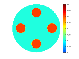
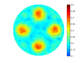
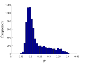
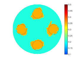
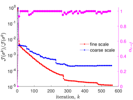
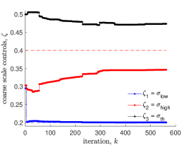
Figure 8: Model #2. (a) True electrical conductivity $\sigma_{true}(x)$. Outcomes for optimization: (b,c) when performed only at a fine scale, and (d,e,f) after applying the multiscale framework by Algorithm 1. Plots in (b,d) show the obtained images with added dotted circles to represent the location of four cancer-affected regions taken from known $\sigma_{true}(x)$. The fine scale solution histogram is presented in (c). Graph in (e) shows normalized cost functional $\mathcal{J}(\sigma^{k})/\mathcal{J}(\sigma^{0})$ as a function of iteration count $k$ evaluated at fine (red dots) and coarse (blue dots) scales. Pink dots show values $\alpha_{c\rightarrow f}$ as solutions for problem (23). Changes in the coarse scale controls $\zeta^{k}=[\sigma^{k}_{low}\ \sigma^{k}_{high}\ \sigma^{k}_{th}]$ are shown in (f) with $\sigma_{c}=0.4$ (red dashed line) and $\sigma_{h}=0.2$ (blue dashed line).

The true electrical conductivity $\sigma_{true}(x)$ for our model #2 containing four same size circular-shaped cancer-affected regions is shown in Figure 8(a). First, we ran a fine scale only optimization for this model which also required more than 1500 iterations to terminate with $\epsilon_{f}=10^{-10}$. As confirmed by the solution image and the associated histogram seen in Figures 8(b,c), we arrived at the same conclusion as for model #1. Even though the high and low conductivity regions are visualized, clear boundaries between them are hardly identifiable. On the other hand, as shown in Figure 8(d) the binary image obtained roughly 3 times faster using multiscale optimization locates all four regions accurately by showing their clear boundaries. Pink and black curves in Figures 8(e,f) show continuous interaction between scales proving the sensitivity of solutions obtained at one scale to changes gained at another one. Relaxation parameter $\alpha_{c\rightarrow f}$ (in pink) different from 1 identifies weighted projections of the coarse scale solutions onto the fine scale performed with weight $1-\alpha_{c\rightarrow f}$. Updated fine scale solutions then are used for constructing fine–to–coarse partitions $\mathcal{M}$ in (14) and (25) by changing values of the coarse scale threshold control $\zeta_{3}=\sigma_{th}$ (in black). We also acknowledge the error in recovering high conductivity part $\hat{\zeta}_{2}=\hat{\sigma}_{high}=0.3466$ due to the high non-linearity of the inverse EIT problem and non-uniqueness of its solution in general, and due to the presence of “equivalent” noise in measurements in particular.

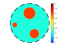
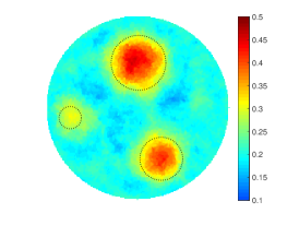
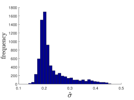
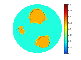
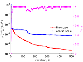
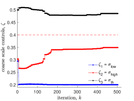
Figure 9: Model #3. (a) True electrical conductivity $\sigma_{true}(x)$ with added structure of boundary electrodes (in black). Outcomes for optimization: (b,c) when performed only at a fine scale, and (d,e,f) after applying the multiscale framework by Algorithm 1. Plots in (b,d) show the obtained images with added dotted circles to represent the location of three cancer-affected regions taken from known $\sigma_{true}(x)$. The fine scale solution histogram is presented in (c). Graph in (e) shows normalized cost functional $\mathcal{J}(\sigma^{k})/\mathcal{J}(\sigma^{0})$ as a function of iteration count $k$ evaluated at fine (red dots) and coarse (blue dots) scales. Pink dots show values $\alpha_{c\rightarrow f}$ as solutions for problem (23). Changes in the coarse scale controls $\zeta^{k}=[\sigma^{k}_{low}\ \sigma^{k}_{high}\ \sigma^{k}_{th}]$ are shown in (f) with $\sigma_{c}=0.4$ (red dashed line) and $\sigma_{h}=0.2$ (blue dashed line).

Our next model #3 contains three circular-shaped cancer-affected regions of various sizes. Its electrical conductivity $\sigma_{true}(x)$ is shown in Figure 9(a). As in the previous case, we run a fine scale only optimization terminated with $\epsilon_{f}=10^{-10}$ which gives a solution image and the associated histogram as shown in Figures 9(b,c). Compared with #2, this model is considered harder as it contains a small spot at the left whose dimension is comparable with the size of the boundary electrodes added in black to Figure 9(a). The image obtained at the fine scale, see Figure 9(b), confirms this complexity as, unlike the two bigger spots, the smallest one lost its color development and, consequently, could be missed. Further analysis of Figures 9(b,c) suggests that clear boundaries between the high and low conductivity regions are hardly identifiable.

Similarly to model #2, Figure 9(d) exhibits results of applying multiscale optimization Algorithm 1 as a clear image of model #3 with a nice binary resolution enabled to locate three cancer-affected regions. Continuous information exchange between fine and coarse scales due to solution projections is also observed in Figures 9(e,f). Here we should comment that the deviated location of the smallest region and the error in recovering high conductivity part of the coarse scale control $\zeta$, $\hat{\zeta}_{2}=\hat{\sigma}_{high}=0.3493$, could be also explained by the high non-linearity of the inverse EIT problem and the presence of the “equivalent” noise. To add more, various size and using $\sigma_{th}$ as a single control for all three regions may significantly contribute to amplify these errors.

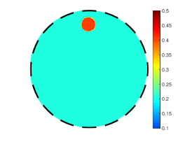
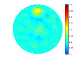
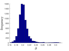
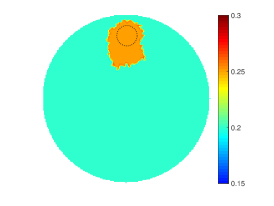
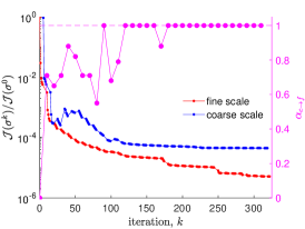
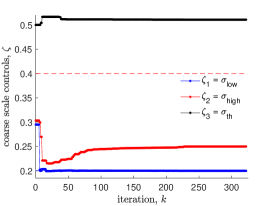
Figure 10: Model #4. (a) True electrical conductivity $\sigma_{true}(x)$ with added structure of boundary electrodes (in black). Outcomes for optimization: (b,c) when performed only at a fine scale, and (d,e,f) after applying the multiscale framework by Algorithm 1. Plots in (b,d) show the obtained images with added dotted circles to represent the location of one small cancer-affected region taken from known $\sigma_{true}(x)$. Graph in (e) shows normalized cost functional $\mathcal{J}(\sigma^{k})/\mathcal{J}(\sigma^{0})$ as a function of iteration count $k$ evaluated at fine (red dots) and coarse (blue dots) scales. Pink dots show values $\alpha_{c\rightarrow f}$ as solutions for problem (23). Changes in the coarse scale controls $\zeta^{k}=[\sigma^{k}_{low}\ \sigma^{k}_{high}\ \sigma^{k}_{th}]$ are shown in (f) with $\sigma_{c}=0.4$ (red dashed line) and $\sigma_{h}=0.2$ (blue dashed line).

Our last model #4 is the hardest one created to mimic using the EIT techniques in medical practice for recognizing cancer at the early stages. The electrical conductivity $\sigma_{true}(x)$ is shown in Figure 10(a). This model contains only one circular-shaped cancer-affected region of the same size as the smallest region in model #3. The known complication comes from the fact that the order of difference in measurements generated by this model and “healthy tissue” ($\sigma(x)=\sigma_{h},\ \forall x\in\Omega$) is very close to the order of noise that appeared naturally in provided data. As for previous models, we compare the results obtained after applying fine scale only optimization, see Figures 10(b,c), and multiscale optimization Algorithm 1, shown in Figures 10(d,e,f), both terminated with $\epsilon_{f}=10^{-10}$.

After comparing fine scale and multiscale optimization images, it is true to say that the latter could provide more assistance in concluding on possible abnormal changes in tissues and navigating the surgeons. On the other hand, the fine scale image may be misleading as some (yellowish) regions may be deceptively interpreted as being cancerous. The multiscale optimization, however, allows keeping its images devoid of this problem and, as such, shows high potential in minimizing possibilities for false positive screening and improving the overall quality of the EIT-based procedures. Similarly to our previous models, the same conclusion arrives after observing continuous information exchange between fine and coarse scales seen in Figures 10(e,f) which results in creating an image with clear binary resolution ready to locate the cancer-affected region. We also note that its size appears larger than in the true model and the error in recovering the coarse scale control $\hat{\zeta}_{2}=\hat{\sigma}_{high}=0.2499$ is much bigger than that seen in the previous models. However, we expect these results may be further improved by applying additional calibration to the (potentially extended) list of chosen parameters, as well as by applying more advanced minimization techniques while performing optimization at both fine and coarse scales.

5 Concluding Remarks

In this work, we presented an efficient computational approach for optimal reconstructing the physical properties of the media characterized by distributions close to binary. In particular, this approach could be useful in various applications in biomedical sciences to operate with physical models supplied with some, possibly incomplete and noisy, measurements. This claim is supported by a simple fact that the proposed multiscale algorithm is given in a very broad context and could be easily applied to other models by changing PDE systems in the formulation of forward and adjoint problems. The proposed computational framework includes an array of gradient-based multiscale optimization techniques supplied with multilevel control space reduction over both fine and coarse scales used interchangeably. Quality and computational efficiency of the obtained results are ensured by developing a methodology for establishing an effective “communication” between scales by projecting the solutions from one scale onto another and accumulating optimally progress obtained at both scales. Such multiscale optimization paired with multilevel control space reduction allows using computational advantages seen at both scales and to mitigate their negative impacts.

We investigated the performance of our complete computational framework in applications to the 2D inverse problem of cancer detection by the Electrical Impedance Tomography technique. Our first benchmark model mimics a simple biological tissue case with confirmed presence of one circular-shaped area affected by cancer. The proposed procedure for calibrating certain parameters was applied to this model to ensure the enhanced performance of our optimization framework. We also presented results obtained by applying the calibrated framework to multiple models of an increased level of complexity, namely with three and for cancer-affected regions of various sizes. For every model, we obtained clear images with a nice binary resolution enabled to locate all cancer-affected regions. In addition, our multiscale optimization framework proved its high efficiency by completing computations 3 times faster than in cases when only fine scale was in use.

We also check the applicability of our framework in applications to procedures for cancer recognition at the early stages by a model containing one tiny cancerous spot with a diameter comparable with the size of the boundary electrodes. Despite the errors in recovering the true shape and the values of electrical conductivity, we conclude that obtained images of that quality will provide valuable assistance in recognizing possible abnormal changes in tissues and further navigating medical professionals with their decisions. We conclude that the properly calibrated multiscale optimization framework is able to provide binary images consistent with the provided measurements using significantly reduced computational time. In general, we see a high potential of the proposed computational framework in minimizing possibilities for false positive screening and improving the overall quality of the EIT-based procedures.

There are many ways in which our multiscale optimization algorithm can be tested and extended. We provided an example of a simple calibration procedure, but we expect the performance may be further improved by extending the list of calibrated parameters and applying more advanced minimization techniques to perform local and global searches while performing optimization at both fine and coarse scales. Given that we used data provided by a specific electrode configuration, it will be of interest to apply a further analysis of the measurement structure, for example considering a 32-electrode scheme and improving sensitivity by optimizing the structure of available data. Also, as many modern EIT systems feature pair-wise voltage patterns, we will be interested in testing the performance of our new method in applications to such systems. We also plan to investigate the use of flexible schemes for switching between scales including new approaches for projecting solutions. The impact of the noise present in measurements should be also systematically analyzed. Also of interest is the extension of our multiscale optimization approach to include possibility of using various PCA sample structures, multiple coarse scale controls associated with different spatial regions, and applicability to bimodal distributions.

Finally, it is important to test our new approach in various applications to real data and different types of cancerous tissues, as this would certainly suggest areas in which further developments may be required. For example, some applications of EIT may require modeling conductivity with more than one different values to characterize “healthy” and ”cancerous” tissues. We expect our new approach could be easily adapted to this and even more complicated settings, e.g. considering electrical conductivity to be considered fully anisotropic, seen in reality. Despite the fact that this approach was initially tested with synthetic EIT-related problems, we believe that this methodology could be easily applied to a broad range of problems in biomedical sciences, also in physics, geology, chemistry, etc.

References

- [1] Abascal, J.F.P.J., Lionheart, W.R.B., Arridge, S.R., Schweiger, M., Atkinson, D., Holder, D.S.: Electrical impedance tomography in anisotropic media with known eigenvectors. Inverse Problems 27(6), 1–17 (2011)
- [2] Abdulla, U.G., Bukshtynov, V., Seif, S.: Breast cancer detection through electrical impedance tomography and optimal control theory: Theoretical and computational analysis. arXiv:1809.05936
- [3] Adler, A., Arnold, J., Bayford, R., Borsic, A., Brown, B., Dixon, P., Faes, T.J., Frerichs, I., Gagnon, H., Gärber, Y., Grychtol, B., Hahn, G., Lionheart, W., Malik, A., Stocks, J., Tizzard, A., Weiler, N., Wolf, G.: GREIT: towards a consensus EIT algorithm for lung images. In: 9th EIT conference 2008, 16-18 June 2008, Dartmouth, New Hampshire. Citeseer (2008)
- [4] Adler, A., Gaburro, R., Lionheart, W.: Handbook of Mathematical Methods in Imaging, chap. Electrical Impedance Tomography, pp. 701–762. Springer New York, New York, NY (2015)
- [5] Alber, M., Tepole, A.B., Cannon, W.R., De, S., Dura-Bernal, S., Garikipati, K., Karniadakis, G., Lytton, W.W., Perdikaris, P., Petzold, L., Kuhl, E.: Integrating machine learning and multiscale modeling – perspectives, challenges, and opportunities in the biological, biomedical, and behavioral sciences. Digital Medicine 2(115) (2019)
- [6] Bera, T.K.: Applications of electrical impedance tomography (EIT): A short review. IOP Conference Series: Materials Science and Engineering 331, 012,004 (2018)
- [7] Berger, M.S.: Nonlinearity and Functional Analysis. Acad. Press, New York (1977)
- [8] Borcea, L.: Electrical impedance tomography. Inverse Problems 18, 99–136 (2002)
- [9] Brown, B.: Electrical impedance tomography (EIT): A review. Journal of Medical Engineering and Technology 27(3), 97–108 (2003)
- [10] Bukshtynov, V., Volkov, O., Durlofsky, L., Aziz, K.: Comprehensive framework for gradient-based optimization in closed-loop reservoir management. Computational Geosciences 19(4), 877–897 (2015)
- [11] Calderon, A.P.: On an inverse boundary value problem. In: Seminar on Numerical Analysis and Its Applications to Continuum Physics, pp. 65–73. Soc. Brasileira de Mathematica, Rio de Janeiro (1980)
- [12] Chen, W., Cheng, J., Lin, J., Wang, L.: A level set method to reconstruct the discontinuity of the conductivity in EIT. Science in China Series A: Mathematics 52, 29–44 (2009)
- [13] Cheney, M., Isaacson, D., Newell, J.: Electrical impedance tomography. SIAM Review 41(1), 85–101 (1999)
- [14] Cheng, K.S., Isaacson, D., Newell, J., Gisser, D.G.: Electrode models for electric current computed tomography. IEEE Transactions on Biomedical Engineering 36(9), 918–924 (1989)
- [15] Clancy, C.E., An, G., Cannon, W.R., Liu, Y., May, E.E., Ortoleva, P., Popel, A.S., Sluka, J.P., Su, J., Vicini, P., Zhou, X., Eckmann, D.M.: Multiscale modeling in the clinic: Drug design and development. Annals of Biomedical Engineering 44(9), 2591–2610 (2016)
- [16] Cominelli, A., Ferdinandi, F., De Montleau, P., Rossi, R.: Using gradients to refine parameterization in field-case history-matching projects. SPE Reservoir Evaluation and Engineering 10(3), 233–240 (2007)
- [17] Davis, T.A.: Algorithm 832: UMFPACK V4.3 – an unsymmetric-pattern multifrontal method. ACM Transactions on Mathematical Software (TOMS) 30(2), 196–199 (2004)
- [18] Gibou, F., Fedkiw, R., Osher, S.: A review of level-set methods and some recent applications. Journal of Computational Physics 353, 82–109 (2018)
- [19] Grimstad, A.A., Mannseth, T.: Nonlinearity, scale, and sensitivity for parameter estimation problems. SIAM Journal on Scientific Computing 21(6), 2096–2113 (2000)
- [20] Grimstad, A.A., Mannseth, T., Nævdal, G., Urkedal, H.: Adaptive multiscale permeability estimation. Computational Geosciences 7, 1–25 (2003)
- [21] Hecht, F.: New development in FreeFem++. Journal of Numerical Mathematics 20(3-4), 251–265 (2012)
- [22] Holder, D.S.: Electrical Impedance Tomography. Methods, History and Applications. CRC Press (2004)
- [23] Horstemeyer, M.F.: Practical Aspects of Computational Chemistry, chap. Multiscale Modeling: A Review. Springer (2009)
- [24] Jolliffe, I.T.: Principal Component Analysis, Second Edition. Springer (2002)
- [25] Jolliffe, I.T., Cadima, J.: Principal component analysis: a review and recent developments. Phil. Trans. R. Soc. A. 374(2065) (2016)
- [26] Lien, M., Berre, I., Mannseth, T.: Combined adaptive multiscale and level-set parameter estimation. Multiscale Modeling & Simulation 4(4), 1349–1372 (2005)
- [27] Lionheart, W.: EIT reconstruction algorithms: Pitfalls, challenges and recent developments. Physiological Measurement 25(1), 125–142 (2004)
- [28] Liu, D., Khambampati, A.K., Du, J.: A parametric level set method for electrical impedance tomography. IEEE Transactions on Medical Imaging 37(2), 451–460 (2018)
- [29] Nocedal, J., Wright, S.J.: Numerical Optimization, 2nd edn. Springer (2006)
- [30] Osher, S., Sethian, J.: Fronts propagating with curvature-dependent speed: Algorithms based on Hamilton-Jacobi formulations. Journal of Computational Physics 79(1), 12–49 (1988)
- [31] Press, W.H., Teukolsky, S.A., Vetterling, W.T., Flannery, B.P.: Numerical Recipes: The Art of Scientific Computing, 3rd edn. Cambridge University Press (2007)
- [32] Steinhauser, M.: Computational Multiscale Modeling of Fluids and Solids: Theory and Applications, 2nd edn. Springer (2017)
- [33] Tai, X.C., Chan, T.: A survey on multiple level set methods with applications for identifying piecewise constant functions. International Journal of Numerical Analysis and Modeling 1(1), 25–47 (2004)
- [34] Tawhai, M., Bischoff, J., Einstein, D., Erdemir, A., Guess, T., Reinbolt, J.: Multiscale modeling in computational biomechanics. IEEE Engineering in Medicine and Biology Magazine 28(3), 41–49 (2009)
- [35] Tsai, R., Osher, S.: Level set methods and their applications in image science. Communications in Mathematical Sciences 1(4), 1–20 (2003)
- [36] Uhlmann, G.: Electrical impedance tomography and Calderón’s problem. Inverse Problems 25(12), 123,011 (2009)
- [37] Volkov, O., Bukshtynov, V., Durlofsky, L., Aziz, K.: Gradient-based Pareto optimal history matching for noisy data of multiple types. Computational Geosciences 22(6), 1465–1485 (2018)
- [38] Walpole, J., Papin, J.A., Peirce, S.M.: Multiscale computational models of complex biological systems. Annual Review of Biomedical Engineering 15, 137–154 (2013)
- [39] Wang, Z., Yue, S., Wang, H., Wang, Y.: Data preprocessing methods for electrical impedance tomography: a review. Physiological Measurement 41(9), 09TR02 (2020)
- [40] Weinan, E.: Principles of Multiscale Modeling. Cambridge University Press (2011)
- [41] Zou, Y., Guo, Z.: A review of electrical impedance techniques for breast cancer detection. Medical Engineering and Physics 25(2), 79–90 (2003)