Accurate mapping of spherically symmetric black holes in a parameterised framework

Abstract

The Rezzolla-Zhidenko (RZ) framework provides an efficient approach to characterize spherically symmetric black-hole spacetimes in arbitrary metric theories of gravity using a small number of variables Rezzolla_Zhidenko14 . These variables can be obtained in principle from near-horizon measurements of various astrophysical processes, thus potentially enabling efficient tests of both black-hole properties and the theory of general relativity in the strong-field regime. Here, we extend this framework to allow for the parametrization of arbitrary asymptotically-flat, spherically symmetric metrics and introduce the notion of a 11-dimensional (11D) parametrization space $\Pi$, on which each solution can be visualised as a curve or surface. An $\mathscr{L}^{2}$ norm on this space is used to measure the deviation of a particular compact object solution from the Schwarzschild black-hole solution. We calculate various observables, related to particle and photon orbits, within this framework and demonstrate that the relative errors we obtain are low (about $10^{-6}$). In particular, we obtain the innermost stable circular orbit (ISCO) frequency, the unstable photon-orbit impact parameter (shadow radius), the entire orbital angular speed profile for circular Kepler observers and the entire lensing deflection angle curve for various types of compact objects, including non-singular and singular black holes, boson stars and naked singularities, from various theories of gravity. Finally, we provide in a tabular form the first 11 coefficients of the fourth-order RZ parameterization needed to describe a variety of commonly used black-hole spacetimes. When comparing with the first-order RZ parameterization of astrophysical observables such as the ISCO frequency, the coefficients provided here increase the accuracy of two orders of magnitude or more.

I Introduction

The Dicke-Eötvös experiment established that the trajectories of freely falling test bodies are independent of their internal structures and compositions, thereby setting the weak equivalence principle (WEP) on firm footing. Truly remarkable tests of whether the speed of light is isotropic and independent of the velocity of the source or not, and tests of time-dilation, conservation of four-momentum, and the relativistic laws of kinematics in particle physics experiments have all bolstered our confidence in the principles of local Lorentz invariance (LLI) and local positional invariance (LPI) as being fundamental features of any serious physical theory. Therefore, the Einstein equivalence principle (EEP), which requires LLI, LPI, and WEP all to hold, is well supported by experiments to date. For further details, we direct the reader to see the foundational papers in experimental gravitation Dicke64 ; Thorne_Will71 , and an excellent modern review can be found in Will14 .

Assuming the exact validity of the EEP implies that metric theories of gravity are the most viable candidates to describe classical gravity, or possibly theories that are metric apart from very weak or short-range non-metric couplings (as in string theory) Dicke64 ; Thorne_Will71 ; Will14 . Following Thorne_Will71 , we define a metric theory as one in which a metric tensor $\bm{g}$ exists and is necessarily associated with gravity, and matter and other non-gravitational fields obey $\bm{\nabla}\cdot\bm{T}=0$, where $\bm{\nabla}$ is defined with respect to the metric $\bm{g}$, and $\bm{T}$ is the energy-momentum-stress tensor for all matter and non-gravitational fields Thorne_Will71 . The latter condition on $\bm{T}$ has the important consequence that test bodies move on geodesics of $\bm{g}$, which is of central importance here Misner+73 . Gravitational redshift, bending of light due to spacetime curvature, frame-dragging effects due to matter currents, and the Shapiro delay are to be expected in any metric theory of gravity, and one can test candidate theories quantitatively, in the weak-field limit, for their agreement with such observables within the parametrized post-Newtonian (PPN) parametrization scheme proposed in Will71a ; Will71b , in terms of 10 variables.

General relativity (GR; Einstein16 ), which is the Ockham’s razor theory of gravity, has withstood all classical weak-field tests to date successfully Will14 ; Collett+18 , and an early success of GR in the strong-field regime was the prediction of the rate of energy loss due to gravitational wave radiation in binary pulsar systems Taylor_Weisberg82 . More recently, with major large-scale astronomy missions such as the Laser Interferometric Gravitational wave Observatory (LIGO) and the Event Horizon Telescope (EHT; Akiyama+19_1 ; Akiyama+19_2 ; Akiyama+19_3 ; Akiyama+19_4 ; Akiyama+19_5 ; Akiyama+19_6 ), it is becoming possible to observe astrophysical events that are dominated by strong-gravity effects. Direct detections of gravitational waves by LIGO from various compact binary systems Abbott+16a ; Abbott+16b and the recently obtained image of the supermassive compact object M87^⋆ by EHT Akiyama+19_1 ; Akiyama+19_2 ; Akiyama+19_3 ; Akiyama+19_4 ; Akiyama+19_5 ; Akiyama+19_6 can be interpreted consistently with the use of the black hole (BH) solutions of GR. The recent observations by GRAVITY of the gravitational redshift Abuter+18 and geodetic orbit-precession Abuter+20 of the star S2 near our galaxy’s central supermassive compact object Sgr A^⋆ are other key successes of GR in strong-gravitational fields.

Various non-BH solutions, such as boson stars and naked singularities, also exhibit many of the features that BH solutions do, such as the presence of photon spheres Olivares+18 ; Shaikh+18 , and characterizing observable differences of such “mimickers” from the BHs of GR is clearly important. Attempting to address the question of the validity of the cosmic censorship hypothesis from an observational point of view is an attractive possibility: while general results like the Birkhoff theorem Birkhoff23 , along with various other analytical Sasaki_Nakamura90 ; Dafermos_Rodnianski10 ; Lucietti_Reall12 ; Duztas_Semiz13 ; Dafermos+14 ; Duztas15 ; Shlapentokh-Rothman15 ; Natario+16 ; Richartz16 and numerical studies Sasaki_Nakamura82 ; Miller_Motta89 ; Yo+02 ; Baiotti+05 ; Nathanail+17 lend weight to our expectation that BHs can, in fact, occur frequently, or equivalently that they do form generically as endstates of continual gravitational collapse, despite significant effort Christodoulou84 ; Christodoulou86 ; Shapiro_Teukolsky92 ; Choptuik93 ; Christodoulou94 ; Christodoulou99b ; Harada+02 ; Crisford_Santos17 we have not been able to rule out the formation of naked singularities in GR.

Of course, the very presence of spacetime singularities, which are locations of arbitrarily large curvatures, in the various solutions of GR is a long standing weakness of the theory. Their existence is assuredly generic Penrose65 ; Penrose69 ; Penrose79 ; Hawking_Ellis73 , and their formation is independent of whether or not they sheathed behind event horizons (see, e.g., Lemaitre33_Tolman34_Bondi47 ; Eardley_Smarr79 ). Therefore, it is useful to study observables associated with regular solutions for BH-like compact objects, both within GR and in alternative theories of gravity, to check whether they are consistent with recent strong-gravity measurements of, e.g., the M87^⋆ shadow size recently obtained by the EHT, and to explore whether they are better models for compact astrophysical objects.

Since the number of models for compact objects offered by various candidate theories of gravity (sometimes when coupled to other fields) is large, when attempting to test the theory of general relativity using strong-field observables, it is imperative that we have a unified theory-agnostic framework ready that characterizes arbitrary solutions (BHs and non-BHs) efficiently, i.e., with as few parameters as possible. Towards this end, we extend here the framework presented in Rezzolla_Zhidenko14 , which can be used to test properties of asymptotically-flat, spherically symmetric BH solutions from arbitrary metric theories of gravity, to include non-BH solutions as well. Our parametrization framework uses 11 parameters and we are able to obtain approximate values for the metrics and various observables, for a variety of compact objects, at typical relative errors of $10^{-6}$. The observables we chose to study here are the orbital angular speeds of test bodies moving on circular geodesics, the impact parameter of photons on unstable circular geodesics (shadow radius), and the angle of deflection due to gravitational lensing; a study of these observables is important when considering the construction of images of compact objects from general-relativistic magnetohydrodynamic (GRMHD) simulations. We also report here the deviations of these observables from their corresponding values for the Schwarzschild BH, for easy comparison.

Finally, since EEP may only hold approximately, i.e., since it could be violated in the strong-field regime (see, e.g., Damour96 ; Damour12 ), it is imperative that the framework we use here to set up strong-field tests of theories of gravity be able to characterize BH solutions from theories that break, e.g., LLI (as in Einstein-aether theories Eling+04 ) or even non-metric theories in which, e.g., the electromagnetic Lagrangian is modified to allow for non-linear interactions Ayon-Beato_Garcia99 . Therefore, the models for compact objects we consider here are: BHs from (a) GR that are either singular Schwarzschild16 ; Reissner16_Nordstrom18 or non-singular Bardeen68 ; Hayward06 ; Held+19 ; Frolov16 , (b) Einstein-aether theory Berglund+12 , (c) string theory Kazakov_Solodhukin94 ; Gibbons_Maeda88 ; Garfinkle+92 ; Garcia+95 ; Casadio+02 , and (d) GR coupled to non-linear electrodynamics Bronnikov01 ; Yajima_Tamaki01 . Additionally, we also consider spacetimes of regular mini boson stars Olivares+18 and naked singularities Janis+68 in GR. We argue that since the level of errors in approximating their exact observables is sufficiently low, it is possible to distinguish between these objects extremely well whenever their exact variables differ, within the present framework.

The outline of the paper is as follows. In Sec. II we discuss a unified framework to parametrize and implement strong- and weak-field tests of arbitrary spherically symmetric metrics in arbitrary metric theories of gravity (and some that are non-metric, as mentioned above). We note that this is a smooth extension of the Rezzolla-Zhidenko parametrization scheme presented in Rezzolla_Zhidenko14 . In Sec. III, we outline how various observables related to causal geodesics may be computed within this parametrization scheme. In Sec. IV, we introduce the notion of a 11D parametrization space $\Pi$ on which every metric solution can be uniquely visualised, and provide brief descriptions of the various compact objects under consideration here. We also demonstrate the efficiency of our framework in obtaining the metric functions (up to two derivatives) across the entire region of interest. For example, for BHs, we are able to approximate their entire exterior geometry to a maximum relative error that is typically less than $10^{-6}$. We also show how all of the associated observables considered here are recovered at similar error levels. Sec. V presents a summary of our results and discusses various advantages of this framework. Our results have considerable overlap with the analysis for BHs presented in Konoplya_Zhidenko20 , and we briefly compare the two sets of results in Sec. V.

II An efficient parametrization framework for spherically symmetric spacetimes

The Rezzolla-Zhidenko (RZ) framework of parameterizing asymptotically-flat, spherically symmetric BH spacetimes in arbitrary metric theories of gravity Rezzolla_Zhidenko14 effectively rewrites a portion of the metric functions in terms of continued-fractions over a conformal radial coordinate. A smooth extension of this scheme was proposed in Konoplya+16 to tackle the problem of parameterizing the broader class of asymptotically-flat, axially-symmetric BH spacetimes, when the metric is expressed in Boyer-Lindquist-like coordinates ($t,r,\theta,\phi$). The existence of the two Killing vector fields $\partial_{t}$ and $\partial_{\phi}$ ensures that the four free metric functions depend only on $r$ and $\theta$, and in the Konoplya-Rezzolla-Zhidenko (KRZ) framework Konoplya+16 , a double-expansion in these variables is employed to parametrize them. In particular, a Taylor expansion in $y=\cos{\theta}$ and a mixed Taylor-Padé expansion in terms of a conformal radial coordinate $x$, similar to the one used here, efficiently parametrizes the exterior horizon geometry. We direct the reader towards Younsi+16 for a demonstration of the efficiency of the KRZ scheme in parameterizing various well known stationary BH metrics and their associated shadow curves.

Restricting to spherically symmetric spacetimes, we now discuss an extension of the RZ scheme that allows for arbitrary asymptotically-flat, static spacetimes, including non-BH ones, to also be similarly characterised.

The line element outside a spherically symmetric configuration of matter can generally be expressed in arbitrary spherical-polar coordinates $(t,\rho,\theta,\phi)$ as

$$\text{d}s^{2}=-f(\rho)\text{d}t^{2}+g(\rho)\text{d}\rho^{2}+h(\rho)\text{d}\Omega_{2}^{2}\,,$$ (1)

where $\text{d}\Omega_{2}^{2}$ is the standard line element of a two-sphere. Since the aim of the current parametrization scheme is to compare metrics across arbitrary metric theories of gravity, it is useful to re-express them in a standardized form, in the same set of “areal-radial, polar” coordinates $(t,r,\theta,\phi)$ as,

$$\text{d}s^{2}=-N^{2}(r)\text{d}t^{2}+\frac{B^{2}(r)}{N^{2}(r)}\text{d}r^{2}+r^{2}\text{d}\Omega_{2}^{2}\,.$$ (2)

This radial coordinate $r$ cleanly determines the proper-area of two-spheres $\mathcal{A}$ in the spacetime as, $\mathcal{A}=4\pi r^{2}$. The desired coordinate transformation $\rho\rightarrow r$ to achieve this change in form can be obtained by solving for $\rho(r)$ from,

$$h(\rho)=r^{2}\,,$$ (3)

with the other metric functions then being given as, $N^{2}(r)=f(\rho(r))$ and $B^{2}(r)=f(\rho(r))g(\rho(r))\left(\partial_{r}\rho(r)\right)^{2}$, where $\partial_{r}$ represents a derivative with respect to $r$.

One can then compactify the radial coordinate by introducing an interior cutoff for it at $r=r_{0}>0$ and defining a conformal radial coordinate $x$ as,

$$x(r)=1-\frac{r_{0}}{r}\,,$$ (4)

and the coordinate patch we will be interested in characterizing here is $r_{0}\!\leq\!r\!<\!\infty$. Clearly, $x(r=r_{0})=0$ and as $r\rightarrow\infty,x(r)\rightarrow 1$. Therefore, characterizing the metric functions $N^{2}(x)$ and $B^{2}(x)$ over the range $0\!\leq x\!<\!1$ is equivalent to fully characterizing the spacetime over this radial range. It is useful to keep in mind the nature of this scale; i.e., a radial range $r_{0}\!<\!r\!<\!2r_{0}$ takes up almost half of the range of the conformal coordinate $0\!<\!x\!<\!.5$. Also, the range $10^{4}r_{0}\!<\!r\!<\!10^{6}r_{0}$ is packed into $1-10^{-4}\!<\!x\!<\!1-10^{-6}$.

When a metric (2) describes the geometry outside a BH, a natural choice for $r_{0}$ exists, namely the location of its event horizon, since one is typically interested in studying features of its exterior geometry. Indeed, this will be our choice here.

Similarly, if one is interested in studying the exterior geometry of a star, one can set $r_{0}$ to correspond to the location of its surface. In the case of a spacetime containing no such natural interior boundary, like that of a boson star or a naked singularity, one can set $r_{0}$ freely to a finite non-zero value. Since the central objective of the present study is to study differences of metric functions and observables associated with various compact objects from the Schwarzschild BH in particular, a convenient choice for $r_{0}$ here, for such objects, is $r_{0}=2M$, where $M$ is the Arnowitt-Deser-Misner (ADM; Arnowitt+62 ) mass of the spacetime. Since we will be considering asymptotically-flat spacetimes exclusively here, identifying $M$ is typically possible. This also reduces the number of requisite parameters from 12 to 11, as we will see below.

As noted above, a fundamental necessity to be able to constrain deviations from GR is a unified theory-agnostic framework that characterizes both the strong- and weak-gravitational field regimes of arbitrary solutions efficiently. Since, by construction, the RZ parametrization scheme handles both these regimes simultaneously and effectively for spherically symmetric BH solutions Rezzolla_Zhidenko14 , a natural choice is to extend it to include non-BH solutions. This is achieved by modifying the auxiliary function $A(x)$ used in Rezzolla_Zhidenko14 as,

$$N^{2}(x)=n_{0}+A(x)x\,,$$ (5)

where $n_{0}=N^{2}(r=r_{0})$. In particular, when the metric (1) describes a BH spacetime we have $n_{0}\!=\!0$, and this definition for $A(x)$ reduces to the one used in equation (4) of Rezzolla_Zhidenko14 . We have essentially modified the “inner”-boundary condition on the 1D box $0\!\leq x\!<\!1$ for the $g_{tt}$-metric function.

For the Killing vector $\partial_{t}$ to remain timelike ($\bm{g}(\partial_{t}\cdot\partial_{t})=g_{tt}<0$) outside the outermost Killing horizon, clearly, we require,

$$0<A(x),\ \ \text{for}\ \ 0\!<x\!<\!1\,.$$ (6)

If a non-BH spacetime admits a Killing surface at some location (perhaps in aether theories), one must set $r_{0}$ to correspond to that location. The non-BH spacetimes considered here do not admit such Killing surfaces, and we will set $r_{0}=2M$ for them in Sec. IV.

Equation (6) implies a continued-fraction approximation for $A(x)$ is already a salient possibility. However, to facilitate an easy comparison with the PPN form of the metric Will71a ; Will14 , we first write out the asymptotic Taylor expansions (to the first few orders) of the metric functions $A$ and $B$, and introduce two new auxiliary functions $\tilde{A}$ and $\tilde{B}$ as,

$$A(x)= \ 1-n_{0}-\epsilon(1-x)+(a_{0}-\epsilon)(1-x)^{2}$$ (7)

$$\quad+\tilde{A}(x)(1-x)^{3}\,,$$

$$B(x)= \ 1+b_{0}(1-x)+\tilde{B}(x)(1-x)^{2}\,.$$ (8)

In the above, we have also introduced three new constants $\epsilon,a_{0}$, and $b_{0}$, which, along with $n_{0}$, can be used to test whether the spacetime in question satisfies the PPN constraints that arise from weak-field tests of gravity, as we will see in Sec. III.1. This redefinition (7, 8) of the auxiliary functions has the consequence that these tilded auxiliary functions, $\tilde{A}$ and $\tilde{B}$, do not influence the values of the PPN parameters of the spacetime.

Thus far, we have roughly performed Taylor expansions of the metric functions when rewritten in terms of $x$ (a variable that behaves as $1/r$) about $x=0$ in equation (5) and $x=1$ in equations (7, 8). At the core of the efficiency of the current parametrization scheme is the choice to characterize $\tilde{A}$ and $\tilde{B}$ as Padé approximants in the form of continued-fractions as,

$$\tilde{A}(x)=\cfrac{a_{1}}{1+\cfrac{a_{2}x}{1+\cfrac{a_{3}x}{1+\cdots}}}\,,\ \ \tilde{B}(x)=\cfrac{b_{1}}{1+\cfrac{b_{2}x}{1+\cfrac{b_{3}x}{1+\cdots}}}\,.$$ (9)

Therefore, the set of PPN coefficients $n_{0},\epsilon,a_{0}$ and $b_{0}$, along with the Padé expansion coefficients, $a_{i}$ and $b_{i}$ ($i>0$), completely characterize arbitrary spherically symmetric spacetimes in arbitrary metric theories of gravity.

By definition, these coefficients $a_{i}\ (i>0)$) can be obtained by Taylor-expanding the continued-fractions in equation (9), and matching the Padé expansion coefficients order-by-order with the Taylor expansion coefficients for $\tilde{A}(x)$, which we write formally as,

$$\tilde{A}(x)=\sum_{i=0}^{\infty}\tilde{a}_{i+1}x^{i}\,.$$ (10)

We show below the first few Padé coefficients of a function $\tilde{A}(x)$ in terms of its Taylor coefficients,

$$a_{1}= \ \tilde{a}_{1}\,,\ \ a_{2}=\ -\frac{\tilde{a}_{2}}{\tilde{a}_{1}}\,,\ \ a_{3}=\ -\frac{\left(\tilde{a}_{3}\tilde{a}_{1}-\tilde{a}_{2}^{2}\right)}{\tilde{a}_{2}\tilde{a}_{1}}\,,$$ (11)

$$a_{4}= \ -\frac{\left(\tilde{a}_{4}\tilde{a}_{2}-\tilde{a}_{3}^{2}\right)\tilde{a}_{1}}{(\tilde{a}_{3}\tilde{a}_{1}-\tilde{a}_{2}^{2})\tilde{a}_{2}}\,,$$

$$a_{5}= \ -\frac{\left(\tilde{a}_{5}\left(\tilde{a}_{3}\tilde{a}_{1}-\tilde{a}_{2}^{2}\right)-\tilde{a}_{4}^{2}\tilde{a}_{1}+2\tilde{a}_{4}\tilde{a}_{3}\tilde{a}_{2}-\tilde{a}_{3}^{3}\right)\tilde{a}_{2}}{\left(\tilde{a}_{4}\tilde{a}_{2}-\tilde{a}_{3}^{2}\right)\left(\tilde{a}_{3}\tilde{a}_{1}-\tilde{a}_{2}^{2}\right)}\,,$$

$$a_{6}= -\frac{\left(\tilde{a}_{6}\left(\tilde{a}_{4}\tilde{a}_{2}-\tilde{a}_{3}^{2}\right)-\tilde{a}_{5}^{2}\tilde{a}_{2}+2\tilde{a}_{5}\tilde{a}_{4}\tilde{a}_{3}-\tilde{a}_{4}^{3}\right)\left(\tilde{a}_{3}\tilde{a}_{1}-\tilde{a}_{2}^{2}\right)}{\left(\tilde{a}_{5}\left(\tilde{a}_{3}\tilde{a}_{1}-\tilde{a}_{2}^{2}\right)-\tilde{a}_{4}^{2}\tilde{a}_{1}+2\tilde{a}_{4}\tilde{a}_{3}\tilde{a}_{2}-\tilde{a}_{3}^{3}\right)\left(\tilde{a}_{4}\tilde{a}_{2}-\tilde{a}_{3}^{2}\right)}\,,$$

to demonstrate that the map between two sets expansion coefficients for the same function is non-linear. The reader may have observed that the dependence of either type of coefficient on the other of the same order is linear.

Henceforth, by an $n^{\text{th}}$-order approximation we will mean that we have truncated the Padé approximants by setting $a_{i>n}=0$. The power of the present parametrization scheme is primarily due to well known property of the rapidity of the order-on-order convergence of Padé approximants (9) to the exact value for a multitude of functions Baker_Graves-Morris96 ; Bender_Orszag99 , as compared to other approximation schemes such as Taylor expansions (10), for example. That this well known efficiency of Padé approximants is carried into the RZ parametrization has been demonstrated for the Einstein-dilaton spacetime Rezzolla_Zhidenko14 , where the rate of convergence of order-on-order truncated Padé approximants was contrasted against the order-on-order truncated Taylor approximations of the Johannsen-Psaltis parametrization scheme in the appendix of Rezzolla_Zhidenko14 . In appendix B below, we conduct a similar convergence test against a recently proposed Taylor expansion-based parametrization scheme Carson_Yagi20 for the Bardeen-BH metric. See also appendix C.

As we will see below in Sec. IV, already at the fourth-order ($a_{5}=b_{5}=0$), we are able to recover both metric functions for various spacetimes with a maximum relative error of about $10^{-6}$ over the entire range $0\leq x<1$, and not just close to the boundaries of the spacetime. In particular, for BH spacetimes, the relative errors are typically far lower at this order. In fact, it has recently been argued that already at the second order one can recover the unstable photon-orbit radius, the orbital angular frequency of the innermost Kepler observer, and the quasi-normal frequency spectrum for scalar perturbations to the desired accuracy for BH solutions that are not close to extremality Konoplya_Zhidenko20 .

For (metric) functions that are fractions of two polynomials, the associated continued-fractions only have a finite (and typically small) number of coefficients $a_{i}$, i.e., for some $n$, all $a_{i>n}=0$, and the $n^{\text{th}}$-order Padé approximant converges exactly to the exact function (see for example the case of the Einstein-aether 1 BH in Sec. IV). However, as can be seen from the cases of the Bronnikov BH and the Janis-Newman-Winicour naked singularity below, even for non-polynomial functions, the Padé approximant still converges fairly rapidly.

Note that it is not always possible to set a particular coefficient $a_{n+1}$ to zero in order to obtain the $n^{\text{th}}$-order truncated Padé approximant. One such instance is easily seen when $a_{n}<-1$; In this case, setting $a_{n+1}=0$ creates a pole at $0\leq x=-1/a_{n}<1$ for the $n^{\text{th}}$-order approximant. To get around such an obstacle, following the discussion in Sec. IV of Konoplya+16 , we may simply set $a_{n+2}=0,a_{n+1}=1$ and obtain then the approximation at the $n^{\text{th}}$-order.

It is now reasonable to ask how small a particular Padé coefficient $a_{n}$ needs to be in order for higher-order coefficients to be neglected. One finds that such zeroes, $a_{n}\rightarrow 0$, are typically associated with poles at the next order, $a_{n+1}\rightarrow\pm\infty$, and it is clear that the combined effect of this zero-pole pair is to send $1+{a_{n}x}/{(1+a_{n+1}x)}\rightarrow 1$. Therefore, we argue that when $|a_{n}|$ is appropriately small, we can set $a_{i\geq n}=0$.

We turn finally to the inner-boundary behaviour of the metric functions in this parametrization scheme. The Taylor expansion of the metric functions near $x=0$ is given as,

$$N^{2}= \ n_{0}+\left(1-n_{0}-2\epsilon+a_{0}+a_{1}\right)x$$ (12)

$$+ \ \left(3\epsilon-2a_{0}-3a_{1}-a_{1}a_{2}\right)x^{2}+O\left(x^{3}\right)\,,$$

$$\frac{B^{2}}{N^{2}}= \ \frac{n_{0}}{\left(1+b_{0}+b_{1}\right)^{2}}$$ (13)

$$+ \ \left(\frac{\left(1-n_{0}-2\epsilon+a_{0}+a_{1}\right)}{\left(1+b_{0}+b_{1}\right)^{2}}+\frac{2n_{0}\left(b_{0}+2b_{1}+b_{1}b_{2}\right)}{\left(1+b_{0}+b_{1}\right)^{3}}\right)x$$

$$+ \ O\left(x^{2}\right)\,.$$

In the case of a BH spacetime ($n_{0}=0$), $x$ measures the distance from the horizon and therefore the above expressions capture the near-horizon geometry of a BH.

We end by noting that the condition given in equation (6) has the effect of setting non-trivial constraints on the allowed ranges of the expansion parameters ${\epsilon,a_{i}}$ for BH solutions, i.e., when working at a particular order $n$, the expansion parameters $\epsilon,a_{i\leq n}$ cannot be freely chosen. This is of considerable importance when employing this parametrization scheme to set up tests by solving inverse problems.

III Characterizing observables in the parametrization scheme

In this section, we outline how various observables associated with spherically symmetric metrics can be obtained within the current parametrization scheme. In particular, we discuss how the PPN parameters, the orbital angular frequency of Kepler observers, and deflection of light due to gravitational lensing can be calculated within this framework. We show also the calculation for the impact parameter of photons on unstable circular geodesics for completeness Rezzolla_Zhidenko14 . In addition to these observables, the method to obtain the quasi-normal frequencies associated with scalar perturbations of spherically symmetric spacetimes within this parametrization scheme can also be found in Rezzolla_Zhidenko14 . We find it useful to note here that of the observables considered here, only the gravitational lensing deflection angle depends on the metric function $B$. When two spacetimes have identical $N^{2}$-functions, this observable can be used to distinguish between the two spacetimes (see for example the instances of the Hayward and Modified Hayward BHs in Sec. IV).

III.1 Testing PPN constraints

The metric functions corresponding to a generic asymptotically-flat spacetime can be expanded around asymptotic infinity, $x=1$, and expressed as,

$$N^{2}= \ 1-\frac{2M}{r_{0}}(1-x)+(\beta-\gamma)\frac{2M^{2}}{r_{0}^{2}}(1-x)^{2}+O\left((1-x)^{3}\right)\,,$$

$$\frac{B^{2}}{N^{2}}= \ 1+\gamma\frac{2M}{r_{0}}(1-x)+O\left((1-x)^{2}\right)\,,$$ (14)

where $\beta$ and $\gamma$ are parameters that can be obtained from the fall-off features of the metric functions. For metric theories, $\beta$ and $\gamma$ are called Parametrized Post-Newtonian (PPN) parameters, and measure respectively, e.g., the agreement of their predictions for the perihelion shift of Mercury and the time delay or light deflection due to the Sun; these satisfy Will14 ,

$$|\beta-1|\lesssim 2.3\times 10^{-4}\,,\ \ |\gamma-1|\lesssim 2.3\times 10^{-5}\,.$$ (15)

The Taylor expansions of the metric functions around the exterior boundary of the spacetime can be obtained as,

$$N^{2}= \ 1-(1-n_{0}+\epsilon)(1-x)+a_{0}(1-x)^{2}+O\left((1-x)^{3}\right)\,,$$

$$\frac{B^{2}}{N^{2}}= \ 1+(1-n_{0}+\epsilon+2b_{0})(1-x)+O\left((1-x)^{2}\right)\,,$$ (16)

and on comparing equations (III.1) and (16), we can identify that,

$$\epsilon=\frac{2M}{r_{0}}-\left(1-n_{0}\right)\,,\ \ a_{0}=\frac{2M^{2}}{r_{0}^{2}}(\beta-\gamma)\,,\ \ b_{0}=\frac{M}{r_{0}}(\gamma-1)\,.$$ (17)

Therefore, the PPN constraints (15) then straightforwardly translate into constraints on the four constants introduced above $n_{0},\epsilon,a_{0}$, and $b_{0}$, as,

$$\mathcal{P}_{1}= \ \left|\frac{2a_{0}}{(1-n_{0}+\epsilon)^{2}}+\frac{2b_{0}}{(1-n_{0}+\epsilon)}\right|\lesssim 2.3\times 10^{-4}\,,$$

$$\mathcal{P}_{2}= \ \left|\frac{2b_{0}}{(1-n_{0}+\epsilon)}\right|\lesssim 2.3\times 10^{-5}\,.$$ (18)

Note that a spacetime with vanishing zeroth-order parameters, $a_{0}$ and $b_{0}$, straightaway satisfies PPN constraints. Furthermore, it is also clear that the functions $\tilde{A}$ and $\tilde{B}$ do not contribute in any capacity towards asymptotic PPN constraints.

For non-BH spacetimes ($n_{0}\neq 0$), if one sets $r_{0}=2M$, then $\epsilon=n_{0}$, and these constraints simplify to $\mathcal{P}_{1}=|2a_{0}+2b_{0}|$ and $\mathcal{P}_{2}=|2b_{0}|$ respectively. Notice that for BH spacetimes, since $n_{0}=0$, the parameter $\epsilon$ must satisfy $\epsilon>-1$ for the horizon to exist ($r_{0}>0$).

We also use the PPN constraints above (III.1) for all of the BH solutions coming from the non-metric theories of gravity used here since (a) for the dilaton BHs, despite the non-metric coupling of the electrodynamics (ED) Lagrangian, photons still move along null geodesics of the metric (2), and (b) for the non-linear ED BHs, the Lagrangian reduces to Einstein-Hilbert-Maxwell in the weak-field limit Ayon-Beato_Garcia99 ; Bronnikov01 ; Yajima_Tamaki01 . We think it useful to mention here also that these BHs have the same asymptotic behaviour as the BHs of GR (up to the relevant orders for PPN considerations). The Einstein-aether BHs considered here have $\beta=\gamma=1$ (see, e.g., Jacobson07 ; Jacobson08 ). Note that we have made the rather strong assumption that even though these theories might not satisfy the Birkhoff theorem these constraints are satisfied by astrophysical BHs.

III.2 Photon and particle orbits

Central to the comparison of images of compact objects that the EHT will obtain, such as Sgr A^⋆, against GRMHD simulations is the study of the flow of matter in accretion disks near such objects, and of the motion of photons in the associated spacetime. As a first approximation, if the motion of accreting matter is modelled as being circularly freely-falling, then a study of timelike stable circular geodesics becomes important. The radial in-fall speed of matter on such orbits is negligible compared to the speed at which it rotates around the compact object. In general, circular Kepler geodesics do not extend all the way into the black hole or up to the surface of a non-BH compact object, and there exists an innermost stable circular orbit (ISCO) at some radius $r=r_{{}_{\text{ISCO}}}$. Matter below this point $r\!<\!r_{{}_{\text{ISCO}}}$ is pulled onto the compact object considerably more quickly. Therefore, local features of the flow of matter differ significantly depending where on the matter is relative to the ISCO, and the angular speed of matter at this location $\Omega_{{}_{\text{ISCO}}}$ sets a dynamical free-fall timescale and constitutes an important observable of the compact object. Since this matter is typically a hot plasma, it emits radiation which is lensed by the gravity of the compact object before it reaches asymptotic observers present on earth for example. Some of these photons are also trapped by the compact object, depending on whether or not it possesses a photon sphere, which can be characterised by the impact parameter of the unstable circular photon orbit $\xi_{\text{ps}}$. Essentially, (radially in-going) photons with impact parameter $\xi\!<\!\xi_{\text{ps}}$ are captured by the central object, and are on unstable orbits, as we will see below. Therefore, the union of the direction of all unstable null geodesics, from the point of view of an asymptotic observer, in a spacetime geometry constitutes its shadow region, and whose boundary is characterised by the photon sphere Hioki_Maeda09 .

In this section, we will show how the Kepler orbital angular frequency profile $\Omega_{\text{K}}(r)$, its ISCO value $\Omega_{{}_{\text{ISCO}}}\equiv\Omega_{\text{K}}(r_{{}_{\text{ISCO}}})$, the light deflection angle due to gravitational lensing $\Delta\phi_{\text{GL}}$, and the impact parameter of the photon on a circular unstable geodesic $\xi_{\text{ps}}$ can be obtained within the present parametrization scheme. Towards this end, we begin with a brief discussion on circular causal geodesics, with particular focus on unstable null and stable timelike ones. Since we are concerned with spherically symmetric spacetimes, a discussion of circular geodesics in the equatorial plane suffices Hioki_Maeda09 .

The Lagrangian describing geodesic motion in a static spacetime (1) is given by

$$2\mathcal{L}=-N^{2}(r)\dot{t}^{2}+\frac{B^{2}(r)}{N^{2}(r)}\dot{r}^{2}+r^{2}\dot{\theta}^{2}+r^{2}\sin^{2}\theta\dot{\phi}^{2}\,,$$ (19)

where the overdot represents a derivative with respect to the affine parameter. Since the Lagrangian is independent of $t$ and $\phi$, one obtains two constants of the motion as,

$$p_{t}:=\frac{\partial\mathcal{L}}{\partial\dot{t}}=-N^{2}\dot{t}=-E\,,\ \ p_{\phi}:=\frac{\partial\mathcal{L}}{\partial\dot{\phi}}=r^{2}\sin^{2}\theta\dot{\phi}=L\,,$$ (20)

where $E$ and $L$ are, respectively, the energy and angular momentum of the observer. We can rewrite equation (19) for geodesics restricted to the equatorial plane ($\theta=\pi/2,\dot{\theta}=0$) as,

$$\frac{B^{2}}{N^{2}}\dot{r}^{2}+\left(\frac{L^{2}}{r^{2}}-\frac{E^{2}}{N^{2}}-2\mathcal{L}\right)=0\,,$$ (21)

where $2\mathcal{L}=0$ for null geodesics and $2\mathcal{L}=-1$ for timelike geodesics. Let us define, for convenience, effective potentials for equatorial null ($V$) and timelike ($\tilde{V}$) observers as,

$$V:= \ E^{2}\left(\frac{\xi^{2}}{r^{2}}-\frac{1}{N^{2}}\right)\,,$$ (22)

$$\tilde{V}:= \ \tilde{E}^{2}\left(\frac{\tilde{\xi}^{2}}{r^{2}}-\frac{1}{N^{2}}+\frac{1}{\tilde{E}^{2}}\right)\,,$$ (23)

where in the above we have introduced the impact parameter of a null observer as $\xi=L/E$ and analogously also the impact parameter $\tilde{\xi}$ of a timelike observer.

Equatorial circular null geodesics satisfy $\dot{r}=0$ and $\ddot{r}=0$, or equivalently $V=0$ and $\partial_{r}V=0$. The stability of a circular null geodesic is governed by the sign of $\partial_{r}^{2}V$ ($-$ implies unstable). The expressions for the first and second derivatives of the effective potential are provided below for later use,

$$\frac{\partial_{r}V}{E^{2}}= \ -2\left(\frac{\xi^{2}}{r^{3}}-\frac{\partial_{r}N}{N^{3}}\right)\,,$$ (24)

$$\frac{\partial_{r}^{2}V}{E^{2}}= \ 6\left(\frac{\xi^{2}}{r^{4}}-\frac{(\partial_{r}N)^{2}}{N^{4}}+\frac{\partial_{r}^{2}N}{3N^{3}}\right)\,.$$

Stability of circular timelike geodesics can be similarly determined and the relevant expressions for $\partial_{r}\tilde{V}$ and $\partial_{r}^{2}\tilde{V}$ for them can be obtained simply by replacing all of the quantities in equation (24) with their tilded counterparts.

III.2.1 Photon sphere impact factor

As discussed above, equatorial circular null geodesics satisfy,

$$0=\frac{\xi^{2}}{r^{2}}-\frac{1}{N^{2}}\,,\ \ 0=\frac{\xi^{2}}{r^{3}}-\frac{\partial_{r}N}{N^{3}}\,.$$ (25)

Equivalently, their radii $r=r_{\text{c}}$ can be found by solving,

$$r-\frac{N(r)}{\partial_{r}N(r)}=0\,.$$ (26)

If $\partial_{r}^{2}V(r=r_{\text{c}})\!<\!0$, the spacetime has an unstable circular null geodesic at that location, and a stable circular null geodesic otherwise. Of these locations, that which corresponds to the absolute maximum of the null geodesic potential $V$ marks the boundary of the shadow.

We will denote this location by $r_{\text{ps}}$. The corresponding impact parameter $\xi_{\text{ps}}$ of a photon on such an orbit is given as,

$$\xi_{\text{ps}}=\frac{r_{\text{ps}}}{N(r_{\text{ps}})}\,.$$ (27)

While the photon sphere marks the boundary of the shadow region of a spacetime, when viewing the compact object from asymptotic infinity, due to gravitational lensing, we see it to be of size $\xi_{\text{ps}}$ Hioki_Maeda09 , which the EHT has observed. In terms of the conformal radial coordinate introduced above, $x=1-r_{0}/r$, we can now find the location of all allowed circular null geodesics by finding the solution $x=x_{\text{c}}$ of the equation Rezzolla_Zhidenko14 ,

$$(1-x)-\frac{N(x)}{\partial_{x}N(x)}=0\,,$$ (28)

where $\partial_{x}$ denotes a derivative w.r.t. $x$. We denote by $x_{\text{ps}}$ the location of the absolute maximum of the null geodesic potential, and the corresponding impact factor of this photon $\xi_{\text{ps}}$ is given as,

$$\xi_{\text{ps}}=\frac{r_{0}}{(1-x_{\text{ps}})N(x_{\text{ps}})}\,.$$ (29)

III.2.2 Orbital angular velocity on stable circular geodesics

The class of equatorial Kepler observers in a static spacetime (1) correspond to stable circular timelike geodesic motion, and satisfy, as discussed above,

$$0=\frac{\tilde{\xi}^{2}}{r^{2}}-\frac{1}{N^{2}}+\frac{1}{\tilde{E}^{2}}\,,\ \ 0=\frac{\tilde{\xi}^{2}}{r^{3}}-\frac{\partial_{r}N}{N^{3}}\,.$$ (30)

From the above, we can straightforwardly obtain the associated equatorial Kepler frequency at a given radius $\Omega_{\text{K}}=\dot{\phi}/\dot{t}$ as,

$$\Omega_{\text{K}}:=\frac{\tilde{\xi}N^{2}}{r^{2}}=\sqrt{\frac{N(r)\partial_{r}N(r)}{r}}\,.$$ (31)

Furthermore, since around sufficiently massive black holes, pulsars (rotating neutron stars that spin around their axes, and emit radiation) can be treated as test objects and are visible to fixed asymptotic observers, measuring the rate at which pulses from them are recorded on earth can be useful towards setting up strong field tests of GR, since this rate depends on the properties of its motion. From pulse profiles of pulsars moving in the vicinity of static black holes, the orbital angular frequency can potentially be extracted, and since this frequency depends on the properties of the central compact object like the mass and charge of the central object, one could in principle extract these parameters for the spacetime as well Kocherlakota+19 .

A particle moving on the ISCO corresponds to the absolute minima of $\tilde{V}_{\text{eff}}$, and satisfies additionally $\partial^{2}_{r}\tilde{V}_{\text{eff}}=0$ i.e.,

$$\frac{\tilde{\xi}^{2}}{r^{4}}-\frac{(\partial_{r}N)^{2}}{N^{4}}+\frac{\partial_{r}^{2}N}{3N^{3}}=0\,.$$ (32)

Clearly, the ISCO is also only marginally stable. The ISCO radius then is the solution of Rezzolla_Zhidenko14 ; DeLaurentis+18 ,

$$3N\partial_{r}N-3r(\partial_{r}N)^{2}+rN\partial_{r}^{2}N=0\,,$$ (33)

and the corresponding orbital angular velocity is given as $\Omega_{{}_{\text{ISCO}}}=\Omega_{\text{K}}(r_{{}_{\text{ISCO}}})$. Kepler observers exist only outside the ISCO i.e., only for $r\geq r_{{}_{\text{ISCO}}}$.

In the current parametrization scheme, the Kepler orbital angular velocity is given by,

$$\Omega_{\text{K}}=\frac{\sqrt{(1-x)^{3}N(x)\partial_{x}N(x)}}{r_{0}}\,,$$ (34)

and the ISCO location is given as $r_{{}_{\text{ISCO}}}=r_{0}/(1-x_{{}_{\text{ISCO}}})$, where $x_{{}_{\text{ISCO}}}$ satisfies,

$$N\partial_{x}N-3(1-x)(\partial_{x}N)^{2}+(1-x)N\partial_{x}^{2}N=0\,.$$ (35)

Finally, the ISCO angular velocity is obtained from equation (34) by setting $x=x_{{}_{\text{ISCO}}}$.

III.2.3 Strong gravitational lensing

We study now the lensing properties of compact objects within this parametrization framework. For equatorial null geodesics, we can characterize the deflection due to gravity via

$$\frac{\text{d}\phi}{\text{d}r}=\frac{\dot{\phi}}{\dot{r}}=\pm\frac{{L}/{r^{2}}}{({N}/{B})\sqrt{{E^{2}}/{N^{2}}-{L^{2}}/{r^{2}}}}=\pm\frac{1}{r^{2}}\frac{B}{\sqrt{1/\xi^{2}-N^{2}/r^{2}}}\,,$$ (36)

where the sign $+$ or $-$ is determined by whether it is out-going ($\dot{r}\!>\!0$) or in-going ($\dot{r}\!<\!0$) respectively. For a null geodesic starting from and ending at asymptotic infinity, the point where it is closest to the compact object, namely its turning point $r=r_{\text{tp}}$, is obtained from the condition that $\dot{r}=0$ there, which gives,

$$\xi=\frac{r_{\text{tp}}}{N(r_{\text{tp}})}\,.$$ (37)

Then, the total deflection due to gravitational lensing $\Delta\phi_{\text{GL}}(r_{\text{tp}})$ of such a null geodesic, i.e., its deviation from a straight line, is given as Weinberg72 ,

$$\Delta\phi_{\text{GL}}(r_{\text{tp}})=2\left|\int^{\infty}_{r_{\text{tp}}}\frac{\text{d}r}{r^{2}}\frac{B(r)}{\sqrt{{N^{2}(r_{\text{tp}})}/{r_{\text{tp}}^{2}}-{N^{2}(r)}/{r^{2}}}}\right|-\pi\,.$$ (38)

Within the current parametrization scheme, this may be rewritten as,

$$\Delta\phi_{\text{GL}}(x_{\text{tp}})=2\left|\int^{1}_{x_{\text{tp}}}\text{d}x\frac{B(x)}{\sqrt{(1-x_{\text{tp}})^{2}N^{2}(x_{\text{tp}})-(1-x)^{2}N^{2}(x)}}\right|-\pi\,,$$ (39)

where $x_{\text{tp}}:=1-{r_{0}}/{r_{\text{tp}}}$. This integral is finite only if the turning point lies outside the photon sphere, i.e., $x_{\text{ps}}\!<\!x_{\text{tp}}\!<\!1$.

In the next section, we display the parameters necessary to parametrize various spacetimes based on the parametrization scheme described in Sec. II and then proceed to demonstrate how efficiently metric functions and the various observables discussed in this section are characterized in this framework.

IV Characterizing spacetimes and observables in the parametrization scheme

We now discuss the conventions used here and the layout of this section before we enter into a brief description of the various BH, boson star, and naked singularity spacetimes considered in this work.

We employ geometrized units throughout $8\pi G=c=1$. Deviations in the gravitational constant $G$ or the Planck length $l_{\text{p}}$ can be measured in scales of their canonical values. Further, since the spacetimes considered here are all asymptotically-flat, the ADM mass $M$ can be used to fix a length scale for the Schwarzschild-like coordinate system used in equation (2). If we switch to a mass-dimensionless radial coordinate $\bar{r}=r/M$, a direct comparison of various quantities (observables and metric functions) associated with various solutions becomes meaningful.

This also allows us to obtain the dependence of various observables associated with the solutions considered here on the other relevant physical “charges”, like the scalar or electric or magnetic charge etc. In instances when the mass of a compact object has been ascertained from observations to requisite precision, one could then potentially look for the dependence on other ADM charges of observational data. The mass-scaling of the various observables considered here is clear from Sec. III. The impact parameter of a photon on an unstable circular orbit $\xi_{\text{ps}}$, the orbital angular frequency for Kepler observers $\Omega_{\text{K}}$, and the deflection angle due to gravitational lensing $\Delta\phi_{\text{GL}}$ scale with mass as $M^{2},M,M^{-1}$ and $M^{0}$ respectively. Further since the conformal parameter $x$ is scale-invariant, the metric functions $N^{2}(x)$ and $B^{2}(x)$ are unaffected i.e., changing the units of the radial coordinate does not affect the Padé expansion coefficients. This is an important quality that makes the definition of a parametrization space $\Pi$ as in Sec. IV.1 useful.

For easy access, the BH metric functions used here have been compiled in table 1. We display in table 2 the parametrization coefficients up to fourth order ($\epsilon,a_{i},b_{i}$ for $0\!\leq\!i\!\leq\!4$) for all solutions considered here, BHs and otherwise. As discussed above, $n_{0}\!=\!0$ for BH spacetimes and $n_{0}=\epsilon$ for non-BH spacetimes since we set the inner boundary in these cases to correspond to the Schwarzschild radius, $\bar{r}_{0}=2$.

In the columns under part I of table 3, we show the relative error in obtaining $\xi_{\text{ps}}$ and $\Omega_{{}_{\text{ISCO}}}$ for various spacetimes, when using Padé approximants truncated at the fourth order ($a_{5}=b_{5}=0$), as an indicative quantitative measure of the ‘goodness’ of the current parametrization scheme. For instance, for a Bardeen BH with specific magnetic charge $\bar{q}_{\text{m}}=0.75$, we get $|1-\xi_{\text{ph};a_{5}=0}/\xi_{\text{ph; exact}}|$ to be $7.35\times 10^{-6}$. We also show the maximum relative error in obtaining the metric functions $N^{2}(x)$ and $B^{2}(x)$ over the entire range $0\!\leq x\!<\!1$. Finally, we display also the maximum relative error in approximating the orbital angular frequency of Kepler observers $\Omega_{\text{K}}$ and the deflection angle due to gravitational lensing $\Delta\phi_{\text{GL}}$ over the entire accretion disk $x_{{}_{\text{ISCO}}}\!<\!x\!<\!1$, where $x_{{}_{\text{ISCO}}}$ is defined via equation (35).

To compare the goodness of the present approximation, we show the exact relative differences from the Schwarzschild values of $\xi_{\text{ps}}$ and $\Omega_{{}_{\text{ISCO}}}$ for various spacetimes under part II of table 3. For example, under the column for impact parameters, we report $|1-\xi_{\text{ps; Spacetime}}/\xi_{\text{ps; Schwarzschild}}|$. We also show the relative error in obtaining the deflection angle due to gravitational lensing at the ISCO radius $\Delta\phi_{\text{GL}}(r_{{}_{\text{ISCO}}})$ there.

Since the relative error levels in obtaining the exact observables within this parametrization scheme are significantly lower when compared to the deviation of their exact values from the Schwarzschild spacetime, setting up precision tests is possible. Furthermore, since the number of parameters to characterize the wide variety of compact objects in use here is small (11), we conclude that this parametrization scheme is a promising framework to test theories of gravity and the quantum field theoretic effects that may show up in astrophysical data related to compact objects. It is remarkable that this parametrization method performs quite well across the entire radial patch, and allows one to capture both weak- and strong-gravitational field regimes simultaneously.

IV.1 Parametrization Space $\Pi$

We now introduce the geometric notion of a parametrization space. If we think of each set of PPN and Padé expansion coefficients $(\epsilon,a_{0\leq i\leq 4},b_{0\leq i\leq 4})$ as being points of some abstract ‘parametrization space’ $\Pi$, then it is clear that for each set of physical charges $q_{j}$ for a given spacetime, we can associate a point $\pi(q_{j})\in\Pi$. As we vary the physical parameters $q_{j}$ associated with that particular spacetime over its entire range, we obtain a curve or surface in $\Pi$, depending on the number of charges, $q_{1},q_{2}\cdots q_{j}$. We can then use the usual Euclidean $\mathscr{L}^{2}$-norm on $\Pi$ to measure distances between such curves or surfaces, or equivalently between solutions. In particular, we define the deviation of a solution from the Schwarzschild BH spacetime, which sits at the origin of this space, as simply being given by,

$$\mathscr{L}^{2}_{0}:=(\pi-0)^{2}=\left(\epsilon^{2}+\sum_{i=0}^{4}(a_{i}^{2}+b_{i}^{2})\right)^{1/2}\,.$$ (40)

Table 2 then lists the coordinates of various spacetimes in this space. When two ‘solution curves’ intersect, the corresponding spacetimes match approximately at the common point. It is to be noted that since we have used only the first few ($n\leq 4$) expansion coefficients to set up $\Pi$, various spacetimes are approximated at varying degrees of accuracy. However since a higher-order approximation does not affect low-order PPN or Padé coefficients, we can always compare spacetimes meaningfully on $\Pi$. For an alternative prescription to measure differences between solutions one may see Suvorov20 , where a superspace approach was adopted.

Now, for each solution, we use a grid with 1000 points for each physical charge, and obtain the PPN and Padé coefficients $\pi(q)$ at each grid point $q$. For the Bardeen BH, there is a single physical parameter $\bar{q}_{\text{m}}$ and we obtain obtain $\pi(\bar{q}_{\text{m}})$ for 1000 points between $0\leq\bar{q}_{\text{m}}\lesssim.76$. We then ascertain whether the PPN constraints (III.1) are met at each grid point and thus obtain the PPN-allowed parameter values for each spacetime. This is reported in table 1. We introduce another useful quantity, the $\mathscr{L}^{\infty}$-norm, which is defined as,

$$\mathscr{L}^{\infty}:= \ \text{max}\left\{|\epsilon|,|a_{i}|,|b_{i}|\ (0\leq i\leq 4)\right\}\,,$$ (41)

to characterize deviations from the Schwarzschild BH solution, and obtain its value at each grid point for a particular spacetime. We can then find the maximum value of $\mathscr{L}^{\infty}_{\text{max}}$ over all the (charge) grid points for a particular spacetime, to obtain a measure of the extent of the region in $\Pi$ that the spacetime has support on. Since all of these solutions become approximately Schwarzschild in the limit of approach to a particular physical parameter value, as can be seen from table 1, $\mathscr{L}^{\infty}_{\text{max}}$ gives a sense of the maximal deviation from the Schwarzschild BH solution. Essentially, if one samples this range of the parameter space along all axes, one is sure to have characterised that particular spacetime. We report $\mathscr{L}^{\infty}_{\text{max}}$ for each spacetime in the last column on table 1 for BHs. Note that for all of the spacetimes considered here, this quantity $\mathscr{L}^{\infty}_{\text{max}}$ is finite. That is, by sampling the region $0<|\epsilon|,|a_{i}|,|b_{i}|\ (0\leq i\leq 4)<10$, we have completely characterised all of the BH spacetimes used in this work. Of course, since the exact value of $\mathscr{L}^{\infty}_{\text{max}}$ depends on the resolution of the grid, we report here a rounded up value as an indicative measure.

For the JNW naked singularity spacetime, we obtain $\mathscr{L}^{\infty}_{\text{max}}\approx 26$ (we use a very coarse grid $\nu=0.1,0.2,\cdots,0.9$ for this spacetime). For each of the boson star models considered here, this number appears to be around $\mathscr{L}^{\infty}_{\text{max}}\approx 10^{3}$. What this means is that all of the spherically symmetric metrics used here lie in a compact region of $\Pi$ around the origin.

Note that we will not restrict our study to the PPN-allowed ranges of the physical charges for the BH spacetimes, reported in table 1, but explore their entire ranges instead.

IV.2 Black Holes

Table 1: Metric functions, $N^{2}(\bar{r})$ and $B^{2}(\bar{r})$, of the BH spacetimes from arbitrary theories of gravity that we have considered. Here, $\bar{r}=r/M$ and $M$ is the ADM mass. The location of the Killing horizon $\bar{r}_{0}$ is obtained by solving $N^{2}(\bar{r}_{0})=0$, and is used in defining the conformal radial coordinate $x=1-\bar{r}_{0}/\bar{r}$. The patch of the spacetime that we capture within this parametrization scheme is the entire exterior horizon geometry, $0\leq x<1$. It is to be noted that for the Einstein-aether BHs, the Killing horizon is different from the actual causal boundary of the BH region. Also, the term $\bar{r}_{-}$ appearing in $B^{2}$ for the Modified Hayward BH is the smaller zero of its $N^{2}$ metric function. We also show below the PPN-allowed range of the relevant parameter for each spacetime. Finally, in the last column we display the (rounded-up) maximum of the absolute values of all expansion coefficients for all PPN-allowed parameter values for a given spacetime, $\mathscr{L}^{\infty}_{\text{max}}$, with its order of magnitude given in square brackets. This number is meant to provide a rough sense of the size of the region of this 11D parameter space on which a particular spacetime of astrophysical interest has support.

Spacetime	Physical Charge	${N^{2}=-g_{00}}$	${B^{2}=-g_{00}g_{11}}$	PPN Constrained	$\mathscr{L}^{\infty}_{\text{max}}$
RN Reissner16_Nordstrom18	$0<\bar{q}\leq 1$	$1-\frac{2}{\bar{r}}+\frac{\bar{q}^{2}}{\bar{r}^{2}}$	1	$0<\bar{q}\lesssim 2.1\times 10^{-2}$	1 [-4]
E-ae 2 Berglund+12	$0<c_{13}<1,$	$1-\frac{2-c_{14}}{\bar{r}}-\frac{(2c_{13}-c_{14})(2-c_{14})^{2}}{8(1-c_{13})}\frac{1}{\bar{r}^{2}}$	1	$0<c_{13}<1,$	8 [-1]
	$0\leq c_{14}\leq 2c_{13}<2$			$0\leq c_{14}\leq 2c_{13}<2$
E-ae 1 Berglund+12	$0<c_{13}<1$	$1-\frac{2}{\bar{r}}-\frac{3^{3}c_{13}}{2^{4}(1-c_{13})}\frac{1}{\bar{r}^{4}}$	1	$0<c_{13}<1$	6 [-1]
Bardeen Bardeen68	$0<\bar{q}_{\text{m}}\leq\sqrt{16/27}$	$1-\frac{2\bar{r}^{2}}{\left(\bar{r}^{2}+\bar{q}_{\text{m}}^{2}\right)^{3/2}}$	1	$0<\bar{q}_{\text{m}}\leq\sqrt{16/27}$	1 [1]
Hayward Hayward06 ; Held+19	$0<\bar{l}\leq\sqrt{16/27}$	$1-\frac{2\bar{r}^{2}}{\bar{r}^{3}+2\bar{l}^{2}}$	1	$0<\bar{l}\leq\sqrt{16/27}$	6 [0]
Bronnikov Bronnikov01	$0<\bar{q}_{\text{m}}\lesssim 1.05$	$1-\frac{2}{\bar{r}}\left(1-\tanh{\frac{\bar{q}_{\text{m}}^{2}}{2\bar{r}}}\right)$	1	$0<\bar{q}_{\text{m}}\lesssim 1.05$	2 [0]
EEH Yajima_Tamaki01	$0<\bar{\alpha},$	$1-\frac{2}{\bar{r}}+\frac{\bar{q}_{\text{m}}^{2}}{\bar{r}^{2}}-\bar{\alpha}\frac{2\bar{q}_{\text{m}}^{4}}{5\bar{r}^{6}}$	1	$0<\bar{\alpha},$	1 [0]
	$0<\bar{q}_{\text{m}}$			$0<\bar{q}_{\text{m}}\lesssim 2.1\times 10^{-2}$
Frolov Frolov16	$0<\bar{l}\leq\sqrt{16/27}$,	$1-\frac{(2\bar{r}-\bar{q}^{2})\bar{r}^{2}}{\bar{r}^{4}+(2\bar{r}+\bar{q}^{2})\bar{l}^{2}}$	1	$0<\bar{l}\leq\sqrt{16/27},$	4 [0]
	$0\leq\bar{q}\leq 1$			$0<\bar{q}\lesssim 2.1\times 10^{-2}$
KS Kazakov_Solodhukin94	$0<\bar{a}$	$-\frac{2}{\bar{r}}+\frac{\sqrt{\bar{r}^{2}-\bar{a}^{2}}}{\bar{r}}$	1	$0<\bar{a}\lesssim 3.0\times 10^{-2}$	4 [-1]
CFM A Casadio+02	$\beta<1$	$1-\frac{2}{\bar{r}}$	$\left(1-\frac{3}{2\bar{r}}\right)\left(1-\frac{4\beta-1}{2\bar{r}}\right)^{-1}$	$|\beta-1|\lesssim 2.3\times 10^{-5}$	3 [0]
CFM B Casadio+02	$1<\beta<5/4$	$1-\frac{2}{\bar{r}}$	$\left(1-\frac{3}{2\bar{r}}\right)\left(1-\frac{4\beta-1}{2\bar{r}}\right)^{-1}$	$|\beta-1|\lesssim 2.3\times 10^{-5}$	3 [0]
Mod. Hayward Frolov16	$0<\bar{l}\leq\sqrt{16/27}$	$1-\frac{2\bar{r}^{2}}{\bar{r}^{3}+2\bar{l}^{2}}$	$\frac{\bar{r}^{6}+\bar{r}_{-}^{6}}{\bar{r}^{6}+\bar{r}_{\text{H}}^{4}\bar{r}_{-}^{2}}$	$0<\bar{l}\leq\sqrt{16/27}$	6 [0]
EMd Gibbons_Maeda88 ; Garfinkle+92 ; Garcia+95	$0<\bar{q}\leq\sqrt{2}$	$1-\frac{\sqrt{4\bar{r}^{2}+\bar{q}^{4}}-\bar{q}^{2}}{\bar{r}^{2}}$	$\frac{4\bar{r}^{2}}{4\bar{r}^{2}+\bar{q}^{4}}$	$0<\bar{q}\lesssim 2.1\times 10^{-2}$	2 [0]

Note that since the mass $M$ is the ADM mass for all of the solutions below, and is a free parameter; We will only discuss the remaining charges in what follows.

The Reissner-Nordström (RN; Reissner16_Nordstrom18 ) BH describes a charged BH in GR, with specific charge $0<\bar{q}\leq 1$.

We consider two BH solutions reported in Berglund+12 that are obtained from the Einstein-aether (E-ae) Lagrangian. In an aether theory, LLI is violated due to the existence of the aether vector field. The first of the two solutions, which we call the E-ae 1 BH is a single parameter solution, $0\!<\!c_{13}\!<\!1$, and the E-ae 2 solution represents a two-parameter family of BHs which take values, $0\!<\!c_{13}\!<\!1$ and $0\!\leq c_{14}\!\leq 2c_{13}\!<\!2$. Here $c_{13}$ and $c_{14}$ are coupling constants that control the aether Lagrangian. It is to be noted that for these spacetimes the causal horizons that separate the BH interiors $B\equiv M-J^{-}(I^{+})$ from their exteriors, called the universal horizons in Berglund+12 , are different from Killing horizons and we use the latter when defining the conformal coordinate $x$.

The Einstein-gravity Lagrangian when coupled to a particular non-linear electrodynamics (NLED) Lagrangian $\mathcal{L}(F)$, which reduces to Maxwell in the weak-field limit, with $F$ the electromagnetic field-strength scalar (see equation 29 of Bronnikov01 ; see also Ayon-Beato_Garcia99 ), yields regular, magnetically-charged BH solutions. These Bronnikov BH solutions are given by equations (3, 11, 30) of Bronnikov01 , with the specific magnetic charge, $0\!<\!\bar{q}_{\text{m}}\!\lesssim\!1.05$, as the only additional charge.

When considering the Einstein Lagrangian coupled to the Euler-Heisenberg (EH) NLED Lagrangian, which is considered to be an effective action of a superstring theory Bern_Morgan94 , one can obtain a magnetically-charged BH solution Yajima_Tamaki01 . This Einstein-Euler-Heisenberg (EEH) BH depends on two parameters, $0\!<\bar{\alpha}$ and $0\!<\!\bar{q}_{\text{m}}$, the former of which is the coupling constant of the $F^{2}$ piece of the EH Lagrangian and is expected to be determined by the string tension $\alpha^{\prime}$ Yajima_Tamaki01 .

It is important to note that due to the self-interaction introduced by the non-linearity of the NLED Lagrangians in the Bronnikov and the EEH BH solutions, photons do not propagate along null geodesics of (2) (see, e.g., the discussion in Stehle_DeBaryshe66 ). However, as was discussed in Cuzinatto+15 , the event horizons are still determined by the zeroes of the null expansions of (2). Therefore, our definition of the conformal coordinate $x$ is unchanged, and we can still characterize these BH spacetimes within the current parametrization scheme. However, other important phenomena such as geometric redshift and light deflection are modified by the NLED Lagrangian. While we are able to show that these solutions are obtained within our parametrization scheme to very high accuracy, and also show that the errors in obtaining the ISCO frequency and the Kepler frequency are also very small (matter is still minimally coupled), we find studying the accuracy in obtaining the photon sphere impact parameter or the deflection of photons due to gravitational lensing for these spacetimes to be beyond the scope of the current article.

The Bardeen-BH model, proposed in Bardeen68 , is the result of the collapse of charged matter, with the usual central singularity replaced by a regular charged matter core. The only relevant parameter in this solution takes values $0\!<\!\bar{q}_{\text{m}}\!\lesssim\!0.77$. More recently, it was shown in Ayon-Beato_Garcia00 that this BH can also be obtained as an exact magnetically-charged solution of an Einstein-NLED Lagrangian.

The Hayward BH model Hayward06 proposes a method to resolve the central singularity in uncharged BHs in GR by adding a region with positive cosmological constant $\Lambda=3/l^{2}$ (de Sitter) close to the centre, where $l$ is the Hubble length. Such a model is expected to be justified by the properties of matter Sakharov66 ; Gliner66 or the quantum theory of gravity Markov82 ; Frolov+90 ; Mukhanov_Brandenberger92 ; Brandenberger+93 close to the centre of the BH. While $l$ provides a length scale for when such effects might set in, and can therefore be related to the Planck length, larger length scales are not strictly excluded. We will consider here the entire range of the parameter for which BH solutions are admitted, $0\!<\!\bar{l}\!\lesssim\!0.77$. Since we have introduced the ADM mass into the definition of $\bar{l}$, which can determined in terms of the canonical values of $G$ and $c$, fixing a particular length scale $l$ can be thought of equivalently as considering BHs within a certain mass range.

The charged generalisation of the Hayward model given by equation (4.1) of Frolov16 is referred to as the Frolov BH here and has an additional parameter which takes values $0\!<\!\bar{q}\!\leq\!1$. Another generalisation of the Hayward model is also presented there, which modifies the redshift function in equations (2.47, 2.50); This we refer to as the modified Hayward model.

The effective dynamics of spherically symmetric fluctuations of the 4D gravitational field can be shown to be governed by a 2D dilaton gravity action Kazakov_Solodhukin94 . By integrating out these fluctuations, one can obtain the (approximate) Kazakov-Solodhukin (KS) BH metric, given in equation (3.18) of Kazakov_Solodhukin94 . The relevant parameter for this solution takes values $0<a$, and determines the area of the singular two-sphere, i.e., $\mathcal{A}_{\text{sing}}=4\pi a^{2}$. While this parameter should be roughly of the order of the Planck length, we allow it to take all positive values here. While, more significantly, non-singular solutions are also presented there, we do not consider them here.

Projecting the 5D vacuum Einstein equations onto a time-like manifold of codimension one (brane) yields the usual ADM Hamiltonian and momentum constraints, for spherically symmetric solutions. If one chooses the four-metric on the brane to be given by equation (2) with $N^{2}(\bar{r})=(1-2/\bar{r})$, this Hamiltonian constraint equation uniquely determines the other metric function, and a one-parameter family of Casadio-Fabbri-Mazzacurati (CFM) BH solutions are obtained, given in equation (8) of Casadio+02 . For $\beta<1$ these are the singular (CFM A) and for $1<\beta<5/4$ these are non-singular (CFM B). The CFM B BHs in fact contain traversable wormholes (the minimal sphere is behind the horizon; see figure 2 of Casadio+02 ). The parameter $\beta$ here corresponds exactly to the PPN $\beta$ parameter.

Due to the coupling of the dilaton field to the electromagnetic field strength $\bm{F}$ in heterotic string theory, the Einstein-Maxwell-dilaton (EMd) BH is the appropriate electromagnetically charged BH solution in the low-energy limit for this theory Gibbons_Maeda88 ; Garfinkle+92 ; Garcia+95 , as opposed to the RN BH. The EMd BH is characterised by the boundary value of the dilaton field $\phi_{0}$ and the specific electric or magnetic charge $\bar{q}$. For convenience, we consider here solutions with $\phi_{0}=0$. In this case, EMd BH solutions exist for $0<\bar{q}\leq\sqrt{2}$.

All BH solutions (barring the NLED BHs, which we have not studied here) cast shadows and all BH solutions admit ISCOs.

Table 2: PPN and Padé approximant coefficients up to order four for various spacetimes. As discussed in the following table 3, at this order, the relative errors in obtaining both the metric functions and various observables is at the level of about $10^{-6}$, and in fact systematically much lower for BHs. For the boson star and naked singularity, we have used $\bar{r}_{0}=2$, and so $n_{0}=\epsilon$. On the other hand, for BHs, $n_{0}=0$. The parameter $\epsilon=2/\bar{r}_{0}-1$ measures the difference of the horizon radius from its Schwarzschild radius for BHs. Also, as was discussed in Sec. III.1 above, $\epsilon,a_{0},b_{0}$ are the only relevant parameters to test whether a particular spacetime is “PPN allowed.” Finally, if a Padé coefficient of some order $n$ vanishes, i.e., if $a_{n\geq 1}=0$ or $b_{n\geq 1}=0$, then the corresponding metric function, $N^{2}$ or $B^{2}$, is exactly characterised within this approximation scheme at order-$n$ (see, e.g., the case of E-ae 1 BHs below).

Black Hole	Physical	PPN coefficients (Taylor)			Higher Order $a$-coefficients (Padé)				Higher Order $b$-coefficients (Padé)
Spacetime	Charge	$\epsilon$	$a_{0}$	$b_{0}$	$a_{1}$	$a_{2}$	$a_{3}$	$a_{4}$	$b_{1}$	$b_{2}$	$b_{3}$	$b_{4}$
Schwarzschild	-	0	0	0	0	0	0	0	0	0	0	0
RN	$\bar{q}=0.5$	0.07180	0.07180	0	0	0	0	0	0	0	0	0
	$\bar{q}=0.9$	0.39286	0.39286	0	0	0	0	0	0	0	0	0
E-ae 2	[0.1, 0.1]	-0.01352	-0.01352	0	0	0	0	0	0	0	0	0
[$c_{13},c_{14}$]	[0.9, 0.1]	-0.51007	-0.51007	0	0	0	0	0	0	0	0	0
	[0.9, 1.7]	-0.10102	-0.10102	0	0	0	0	0	0	0	0	0
E-ae 1	$c_{13}=0.5$	-0.07666	0	0	0.07666	0	0	0	0	0	0	0
	$c_{13}=0.9$	-0.26982	0	0	0.26982	0	0	0	0	0	0	0
Bardeen	$\bar{q}_{\text{m}}=0.25$	0.02471	0	0	0.00100	0.46236	-0.54081	0.04101	0	0	0	0
	$\bar{q}_{\text{m}}=0.75$	0.53960	0	0	0.32920	-0.07610	3.42051	-3.89389	0	0	0	0
Hayward	$\bar{l}=0.25$	0.01641	0	0	-0.01561	-0.09932	0.70929	-0.40533	0	0	0	0
	$\bar{l}=0.75$	0.33333	0	0	-0.08333	-3.75000	3.46667	-0.15897	0	0	0	0
Bronnikov	$\bar{q}_{\text{m}}=0.5$	0.07167	0.07178	0	0.00011	-0.00538	0.33468	-0.33299	0	0	0	0
	$\bar{q}_{\text{m}}=1.05$	1.03616	1.14273	0	0.08279	-0.36596	0.44373	-0.30767	0	0	0	0
EEH	[1, 0.05]	0.79539	0.80585	0	0.03140	1.00000	-0.66667	0.16667	0	0	0	0
$[\bar{q}_{\text{m}},\bar{\alpha}]$	[1,1]	0.48364	0.55030	0	0.19997	1.00000	-0.66667	0.16667	0	0	0	0
Frolov	[0.5, 0.25]	0.09732	0.07526	0	-0.02039	-0.15602	0.74279	-0.37350	0	0	0	0
[$\bar{q},\bar{l}$]	[0.5, 0.6]	0.36454	0.11637	0	-0.09263	-2.39466	2.33431	-0.20990	0	0	0	0
	[0.9, 0.25]	0.61799	0.53013	0	-0.04369	-1.59541	1.85133	-0.17365	0	0	0	0
KS	$\bar{a}=1$	-0.10557	-0.10000	0	0.00689	0.34416	0.32590	-0.22973	0	0	0	0
	$\bar{a}=10$	-0.80388	-0.48077	0	2.97202	17.9580	8.72455	16.6646	0	0	0	0
CFM A	$\beta=-0.9$	0	0	-0.95000	0	0	0	0	0.29100	-0.80649	0.94227	1.09107
	$\beta=0.9$	0	0	-0.05000	0	0	0	0	-0.10485	2.12935	0.03647	2.39174
CFM B	$\beta=1.1$	0	0	0.05000	0	0	0	0	0.24099	4.93512	0.09874	4.23521
	$\beta=1.2$	0	0	0.10000	0	0	0	0	1.13607	13.6579	1.56198	9.44727
Mod. Hayward	$\bar{l}=0.25$	0.01641	0	0	-0.01561	-0.09932	0.70929	-0.40533	-0.00919	3.91749	-2.52087	0.52343
	$\bar{l}=0.75$	0.33333	0	0	-0.08333	-3.75000	3.46667	-0.15897	-0.12939	2.05606	-3.40434	1.48027
EMd	$\bar{q}=0.7$	0.15087	0.16225	0	-0.00011	0.48046	-0.52013	0.01976	-0.00979	-0.02928	0.49677	-0.50314
	$\bar{q}=1.4$	6.07107	24.5000	0	-13.3186	-0.68426	0.05403	-0.99713	-0.72270	-1.64581	0.44380	-0.45354
MBS A	-	0.25607	-2860.02	0	2860.11	-0.99991	-0.00005	-1.03642	-0.33233	-0.54166	1.75930	-2.45991
MBS B	-	0.49436	-2860.02	0	2860.58	-0.99991	0.00007	-0.33170	-0.26234	-1.55777	0.57086	-0.71121
JNW	$\nu=0.1$	0.59869	0	0	0.92739	-1.14757	0.14701	-0.58785	-0.86869	-1.82005	0.47494	-0.47888
	$\nu=0.5$	0.22527	0	0	0.04698	3.34168	-4.35047	0.52143	-0.62883	-0.79818	1.41593	-1.78545
	$\nu=0.9$	0.06345	0	0	-0.23279	2.18778	-2.43883	4.30862	-0.42314	4.60772	-3.49652	4.07833

IV.3 Boson Stars

Spherically symmetric solutions of the Einstein-Klein-Gordon Lagrangian with a quadratic potential can be used to model mini boson stars (MBS; Kaup68 ). Since the matter (scalar field) constituting the MBS, in principle, extends all the way to infinity, albeit with the scalar field density decaying rapidly, these objects lack a sharp boundary or surface, and also permit stable circular orbits all the way to the centre of the spacetime. MBSs can be extremely compact with the 99%-compactness parameter $\mathcal{C}_{99}=M_{99}/R_{99}$ reaching values of about 0.08, where $R_{99}$ is the radius within which 99% of the mass ($M_{99}$) is contained. This parameter is a good measure of how compact an astrophysical object without a surface is; to compare, for a Schwarzschild BH this value is $0.5$. Here we use the two MBS models, denoted A and B, that were numerically obtained and studied in Olivares+18 . These have compactnesses of $0.064$ and $0.07$, and lie on the unstable and stable boson star branches respectively. Since from about a few tens of Schwarzschild radii, these spacetimes look identical to that of the Schwarzschild BH, the associated PPN parameters $\beta$ and $\gamma$ are identical to the Schwarzschild BH values. Also, these models lack photon spheres and regions close to the centre contribute to the image of the boson star Olivares+18 . However, it is discussed there that due to lower densities at the centre in these models, a relatively dark region may be discernible.

Table 3: Under part I of this table, we demonstrate the efficiency of the current parameterisation scheme by reporting the maximum relative error, at fourth order, in approximating the metric functions of various metrics and the associated observables. Typically the relative error drops by more than an order of magnitude order-on-order due to the use of Padé approximants (see table 5 below), and at this order already the typical errors are at the level of $10^{-6}$. Since this parametrization scheme converges rapidly with increasing order of approximation, those few entries that are of relatively low accuracy will be improved by adding a few higher-order coefficients. The convention we use below is that if a number is smaller than $10^{-10}$, we set it to zero. For brevity, we the display the order of magnitude within square brackets. Furthermore, since one of the objectives of such a parametrization scheme is to test theories of gravity, we think it useful to report the relative difference in the exact values of important observables for a particular spacetime from the corresponding values for the Schwarzschild BH, under part II, i.e., we use the exact metric functions for part II.

Spacetime	Physical	I						II
	Charge	Maximum relative error						Exact Deviation from Schwarzschild
		$|\sigma|=\left|1-O_{\text{approx}}/O_{\text{exact}}\right|$						$\delta=1-O_{\text{exact}}/O^{\text{Schw}}_{\text{exact}}$
		$N^{2}[x)$	$B^{2}[x)$	$\xi_{\text{ps}}$	$\Omega_{{}_{\text{ISCO}}}$	$\Omega_{\text{K}}[x)$	$\Delta\phi_{\text{GL}}[x)$	$\xi_{\text{ps}}$	$\Omega_{{}_{\text{ISCO}}}$	$\Delta\phi_{\text{GL}}(r_{{}_{\text{ISCO}}})$
RN	$\bar{q}=0.5$	0	0	0	0	0	2.37 [-7]	4.39 [-2]	-8.21 [-2]	-6.67 [-2]
	$\bar{q}=0.9$	0	0	0	0	0	1.12 [-7]	1.69 [-1]	-3.88 [-1]	-3.28 [-1]
E-ae 2	[0.1, 0.1]	0	0	0	0	0	2.95 [-8]	4.13 [-2]	-3.60 [-2]	1.27 [-2]
$[c_{13},c_{14}]$	[0.9, 0.1]	0	0	0	0	0	7.42 [-8]	-6.71 [-1]	5.94 [-1]	4.87 [-1]
	[0.9, 1.7]	0	0	0	0	0	1.09 [-7]	8.39 [-1]	-4.86 [0]	9.61 [-2]
E-ae 1	$c_{13}=0.5$	0	0	0	0	0	8.58 [-8]	-2.77 [-2]	4.98 [-2]	5.04 [-2]
	$c_{13}=0.9$	0	0	0	0	0	1.49 [-7]	-1.55 [-1]	2.50 [-1]	2.43 [-1]
Bardeen	$\bar{q}_{\text{m}}=0.25$	0	0	0	1.49 [-9]	0	1.20 [-7]	1.06 [-2]	-2.16 [-2]	-2.10 [-2]
	$\bar{q}_{\text{m}}=0.75$	1.78 [-5]	0	7.35 [-6]	2.21 [-5]	1.33 [-5]	3.18 [-5]	1.20 [-1]	-2.86 [-1]	-2.92 [-1]
Hayward	$\bar{l}=0.25$	4.77 [-7]	0	1.20 [-7]	2.56 [-6]	6.53 [-7]	8.89 [-6]	4.71 [-3]	-8.56 [-3]	-8.76 [-3]
	$\bar{l}=0.75$	2.88 [-4]	0	1.29 [-4]	2.26 [-4]	2.28 [-4]	6.86 [-4]	5.03 [-2]	-9.25 [-2]	-9.65 [-2]
Bronnikov	$\bar{q}_{\text{m}}=0.5$	0	0	$\times$	0	0	$\times$	$\times$	-8.20 [-2]	$\times$
	$\bar{q}_{\text{m}}=1.05$	2.58 [-7]	0	$\times$	2.95 [-8]	1.31 [-7]	$\times$	$\times$	-7.15 [-1]	$\times$
EEH	[1, 0.05]	1.74 [-5]	0	$\times$	4.44 [-7]	9.66 [-6]	$\times$	$\times$	-5.90 [-1]	$\times$
$[\bar{q}_{\text{m}},\bar{\alpha}]$	[1, 1]	8.69 [-5]	0	$\times$	2.22 [-4]	7.14 [-5]	$\times$	$\times$	-5.76 [-1]	$\times$
Frolov	[0.5, 0.25]	1.01 [-6]	0	2.66 [-7]	4.37 [-6]	1.19 [-6]	2.54 [-6]	4.99 [-2]	-9.42 [-2]	-7.92 [-2]
$[\bar{q},\bar{l}]$	[0.5, 0.6]	1.82 [-4]	0	7.87 [-5]	1.59 [-4]	1.41 [-4]	2.02 [-3]	8.34 [-2]	-1.63 [-1]	-1.51 [-1]
	[0.9, 0.25]	3.15 [-5]	0	1.47 [-5]	3.80 [-6]	1.94 [-5]	4.71 [-5]	1.83 [-1]	-4.27 [-1]	-3.70 [-1]
KS	$\bar{a}=1$	2.74 [-7]	0	6.66 [-8]	1.45 [-6]	3.81 [-7]	8.68 [-7]	-7.82 [-2]	1.23 [-1]	9.86 [-2]
	$\bar{a}=10$	1.70 [-2]	0	8.62 [-3]	4.34 [-2]	1.53 [-2]	2.38 [-2]	-2.59 [0]	8.81 [-1]	7.52 [-1]
CFM A	$\beta=-0.9$	0	1.16 [-3]	0	0	0	6.35 [-3]	0	0	7.28 [-1]
	$\beta=0.9$	0	5.01 [-7]	0	0	0	3.38 [-7]	0	0	5.43 [-2]
CFM B	$\beta=1.1$	0	5.40 [-6]	0	0	0	2.27 [-6]	0	0	-5.72 [-2]
	$\beta=1.2$	0	1.87 [-3]	0	0	0	4.40 [-4]	0	0	-1.18 [-1]
Mod. Hayward	$\bar{l}=0.25$	5.03 [-7]	2.93 [-4]	1.20 [-7]	2.56 [-6]	6.53 [-7]	2.78 [-4]	4.71 [-3]	-8.56 [-3]	-8.74 [-3]
	$\bar{l}=0.75$	2.93 [-4]	4.73 [-3]	1.29 [-4]	2.26 [-4]	2.28 [-4]	2.60 [-3]	5.03 [-2]	-9.25 [-2]	-9.64 [-2]
EMd	$\bar{q}=0.7$	0	9.69 [-9]	0	0	0	7.54 [-8]	8.67 [-2]	-1.72 [-1]	-1.37 [-1]
	$\bar{q}=1.4$	1.76 [-2]	2.21 [-2]	7.22 [-3]	6.84 [-3]	4.71 [-3]	3.77 [-2]	5.36 [-1]	-3.18 [0]	-3.19 [0]
MBS A	-	3.85 [-4]	2.01 [-2]	$\times$	$\times$	0	-	$\times$	$\times$	$\times$
MBS B	-	5.09 [-2]	5.95 [-2]	$\times$	$\times$	0	-	$\times$	$\times$	$\times$
JNW	$\nu=0.1$	2.10 [-3]	4.30 [-2]	$\times$	$\times$	5.64 [-3]	1.57 [-2]	$\times$	$\times$	$\times$
	$\nu=0.5$	2.00 [-3]	4.54 [-3]	$\times$	7.81 [-3]	9.53 [-4]	9.21 [-4]	$\times$	4.14 [-1]	1.80 [-1]
	$\nu=0.9$	1.40 [-3]	3.50 [-3]	6.95 [-4]	1.11 [-3]	6.65 [-4]	2.91 [-4]	1.18 [-2]	1.88 [-2]	7.72 [-3]

IV.4 The Janis-Newman-Winicour Naked Singularity

The Janis-Newman-Winicour (JNW) spacetime is also obtained as a solution of the Einstein-Klein-Gordon Lagrangian Janis+68 , and can be expressed more simply as in Virbhadra97 . The JNW solution, when written in the form given in equation (1), has metric functions Virbhadra97 ,

$$f(\rho)=g^{-1}(\rho)=\left(1-\frac{2M}{\rho\nu}\right)^{\nu}\,,\ \ h(\rho)=\rho^{2}\left(1-\frac{2M}{\rho\nu}\right)^{1-\nu}\,,$$ (42)

The parameter $\nu$ governs the strength of the scalar field and is given in terms of the specific scalar charge $\bar{\Phi}$ as, $\nu=\left(1+\bar{\Phi}^{2}\right)^{-1/2}$. Clearly, depending on the strength of the scalar field, $0<\nu<1$. The JNW spacetime contains a strong curvature singularity at $\rho=2M/\nu$, which can be seen by computing its Kretschmann scalar $\mathcal{K}=R^{abcd}R_{abcd}$, which diverges there.

It can be straightforwardly seen that $h(\rho)$ is a bijective function (in fact, it is monotonically increasing) for all $\nu$, which allows us to recast the JNW metric into the presently desired form (2). In terms of the polar-areal radial coordinate $r$, it can be verified that the curvature singularity is now at $r=0$ and has zero proper area.

Since the coordinate transformation equation (3) for the JNW spacetime,

$$\bar{\rho}^{2}\left(1-\frac{2}{\bar{\rho}\nu}\right)^{1-\nu}=\bar{r}^{2}\,,$$ (43)

is typically transcendental in nature, we solve for $\bar{\rho}(\bar{r})$ numerically. In the above, we have switched to dimensionless coordinates, $\bar{\rho}=\rho/M$ and $\bar{r}=r/M$. For values of $\nu=0.1,0.3,\cdots,0.9$, we use a uniform grid in $\log{\bar{r}}$, with 100 points per decade to solve equation (43). For these values, equation (43) reduces essentially to finding the roots of a high-degree polynomial. The grid extends from an outer radius $\bar{r}_{\text{max}}=10^{7}$ down to an inner radius $\bar{r}_{\text{min}}=10^{-2}$. The inner grid point is sufficiently small for our purposes since we are interested in the radial range $2\leq\bar{r}<\infty$.

It has been shown that this spacetime contains a photon sphere for $0.5<\nu$ Patil_Joshi12 . For $1/\sqrt{5}\leq\nu<0.5$, two timelike marginally outer/inner stable circular orbits exist at $\bar{r}_{{}_{\text{OSCO}}}$ and $\bar{r}_{{}_{\text{ISCO}}}$; stable circular orbits extend all the way from the centre to $\bar{r}=\bar{r}_{{}_{\text{OSCO}}}$ and from $\bar{r}=\bar{r}_{{}_{\text{ISCO}}}$ to infinity. For $0.5\leq\nu<1$, a single marginally stable circular orbit remains at $\bar{r}=\bar{r}_{{}_{\text{ISCO}}}$ and stable circular orbits exist only outside this location. Using the results of Patil_Joshi12 ; Chowdhury+12 , we can find the locations of the photon sphere and the timelike marginally stable circular orbits in polar-areal radial coordinates to be,

$$\bar{r}_{\text{ps}}= \ \left(\frac{1+2\nu}{\nu}\right)\left(1-\frac{2}{1+2\nu}\right)^{\frac{1-\nu}{2}},$$ (44)

$$\bar{r}_{{}_{\text{ISCO/OSCO}}}= \ \left(\frac{1+3\nu\pm\sqrt{5\nu^{2}-1}}{\nu}\right)\left(1-\frac{2}{1+3\nu\pm\sqrt{5\nu^{2}-1}}\right)^{\frac{1-\nu}{2}},$$

In obtaining the above, we have simply used equation (43). We are able to numerically recover $\bar{r}_{\text{ps}}$ and $\bar{r}_{{}_{\text{ISCO}}}$ with a relative error of about $10^{-6}$ from the exact values reported in equation (44). Note however that we are unable to obtain the photon sphere or ISCO radius when $\bar{r}_{\text{ps}},\bar{r}_{{}_{\text{ISCO}}}<\bar{r}_{\text{min}}$. This, however, corresponds to a very small range of $0\!<\!\nu\!<\!1$. Since the JNW metric has not (commonly) been reported in polar-areal coordinates, we think it useful to display its metric functions for various values of the scalar field parameter $\nu$ and $M=1$, in figure 1.

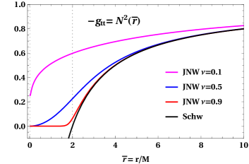
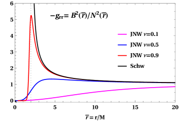
Figure 1: We show here the metric functions $g_{tt}=-N^{2}(\bar{r})$ and $g_{rr}=M^{2}B^{2}(\bar{r})/N^{2}(\bar{r})$ for the JNW naked singularity spacetime for various values of the scalar field parameter, $\nu=0.1,0.5,0.9$. The strength of the scalar field grows with decreasing $\nu$. We also show these metric functions for the Schwarzschild BH for comparison. For both spacetimes, we have set $M=1$.

Once we obtain $N^{2}(\bar{r})$ and $B^{2}(\bar{r})$, we make the final change of coordinates to $x=1-2/\bar{r}$ and obtain the parametrization coefficients, which we report in table 2. Finally, it can be checked that the PPN parameters $\beta$ and $\gamma$ for this spacetime vanish identically for all $\nu$.

V Discussion and Summary

We have proposed here an extension to the RZ parametrization scheme to allow for the characterization of arbitrary asymptotically-flat, spherically symmetric spacetimes, including those of stars and naked singularities. Within this scheme, we obtain highly-accurate values for the metric functions for a variety of spacetimes: singular and non-singular BHs from general relativity, BHs from the Einstein-aether theory, black holes from general relativity coupled to non-linear electrodynamics, string-inspired BH and wormhole solutions, and mini boson stars and naked singularities in general relativity. Various other BH solutions (and including some here) have already been studied within this parametrization scheme and its efficiency in obtaining various observables has been well established Kokkotas+17a ; Kokkotas+17b ; Konoplya_Zhidenko19 ; see also Konoplya_Zhidenko20 and references therein). Recently, an extension of the RZ parameterization framework to characterize spherically symmetric BHs in higher dimensions has also been proposed Konoplya+20 .

The shadow radii $\xi_{\text{ph}}$ of compact objects and the Kepler orbital angular velocities $\Omega_{\text{K}}$ matter in the accretion disks around them depend only on the $g_{tt}$-component of the corresponding metric. Therefore accurate measurements of these observables could be translated into constraints on the $\epsilon$ and $a$ parameters considered here. Additionally, the profile of the gravitational lensing angle $\Delta\phi_{\text{GL}}(r)$ for photons emitted from the accretion disk region depends also on the $g_{rr}$-component, and when combined with the other observables used here, could constrain the entire metric of spherically symmetric (or slowly-rotating) astrophysical compact objects. Other observables such as the quasi-normal frequencies associated with a compact object also depend on both metric functions (see equation 49 of Rezzolla_Zhidenko14 for scalar perturbations), and combined constraints coming from all of these observables can be simultaneously imposed in the present framework to potentially test the underlying theories of gravity.

We have shown above that by sampling the region $0<\epsilon,|a_{i}|,|b_{i}|\ (0\leq i\leq 4)<10$, we have completely characterised all of the BH spacetimes used in this work. This is useful when attempting to solve the inverse problem of reconstructing a metric function approximately given a set of observables that can essentially be determined in terms of these variables, or equivalently as functions over $\Pi$. Note however that these parameters may not be chosen freely. For example, for BHs the conditions $\epsilon>-1$ and $A(x)>0$ over $0<x<1$ must always be satisfied.

If the exact relative difference in an observable $O$ for a spacetime from its Schwarzschild BH value $O^{0}$ is given as $\delta=1-O/O^{0}$ and the relative error in approximating the value of $O$ is given by $\sigma=1-O_{\text{approx}}/O$, then,

$$\delta_{\text{approx}}\equiv 1-\frac{O_{\text{approx}}}{O^{0}}=\delta+\sigma(1-\delta)\,,$$ (45)

and so the absolute error in obtaining $\delta$ is,

$$\delta_{\text{approx}}-\delta=\sigma(1-\delta)\,.$$ (46)

Note that $\delta$ need not be a small number; for spacetimes that deviate significantly from the Schwarzschild BH, $\delta$ can be large (see table 3). However, the absolute error in obtaining $\delta$ due to approximation is clearly controlled by $\sigma$. As we can see from table 3, where we display both $|\sigma|$ and $\delta$, for the spacetimes considered here, $|\sigma|$ is systematically low, about $10^{-6}$. For various spacetimes, it is significantly lower. This means that the error in determining whether, and how different, a particular spacetime is from the Schwarzschild BH using EHT-observables within the present parameterisation scheme is appreciably low. Since this framework employs Padé approximants, the typical order-on-order decrease in $|\sigma|$ is about $10^{-1}\!-\!10^{-2}$, as can be seen from figure 2 of Appendix B below. Therefore, we are able to argue comfortably that the current framework is useful to visualise and compare various spacetimes (in terms of the parametrization space $\Pi$ introduced above), characterise various strong-field observables associated with them, and to enable efficient tests of both properties of BHs from general relativity and GR itself.

Various BH solutions considered here Bardeen68 ; Hayward06 ; Berglund+12 ; Kazakov_Solodhukin94 ; Casadio+02 ; Garcia+95 ; Gibbons_Maeda88 ; Garfinkle+92 ; Bronnikov01 ; Yajima_Tamaki01 were recently studied within the same framework Rezzolla_Zhidenko14 at first- and second-order in Padé expansion Konoplya_Zhidenko20 . It was reported there that all of these solutions, for moderate deviations from the Schwarzschild solution, are well approximated already at second order. While our findings are consistent with those of Konoplya_Zhidenko20 , since the aim of the present study is to explore the entire parameter range for these BH solutions, and errors within this parametrization scheme typically grow with deviation from Schwarzschild (as can be seen from table 3 above and table 4 in Appendix C below), it becomes imperative that we consider higher-order approximations. As has been discussed above, we find that at the fourth-order errors in approximating metric functions and observables are sufficiently low across the entire parameter range for all BH solutions. Furthermore, our PPN constraint study shows that many of the BH spacetimes considered here (Bardeen, Hayward, Modified Hayward) satisfy the PPN constraints across their entire parameter range (see table 1), and parameterizing BHs that deviate significantly (close to their maximal deviation even) from the Schwarzschild solution becomes important from an observational standpoint. Also, to bring the error in approximating the deflection angle due to gravitational lensing $\Delta\phi_{\text{GL}}(r)$ across the entire accretion disk $r_{{}_{\text{ISCO}}}\!\leq\!r$ to sufficiently low levels, we find a fourth-order approximation to be typically necessary. A comparison between the errors reported in Konoplya_Zhidenko20 with those reported here when approximating the ISCO orbital angular velocity $\Omega_{{}_{\text{ISCO}}}$ also demonstrates the rapidity of the convergence to the true value by going to higher orders within the current framework, due to its use of Padé approximants. The relative error levels $|\sigma|$ reported here are typically a few orders of magnitude smaller than the ones reported in Konoplya_Zhidenko20 , as can be seen from table 5 of Appendix C below. For example, the errors in approximating $\Omega_{{}_{\text{ISCO}}}$ for the common BH solutions vary between $0.2-10.5\%$ and $0.04-7.95\%$ at first-and second-order Konoplya_Zhidenko20 , while the maximum percentage error at fourth-order is about $10^{-4}\%$ for moderate deviations from the Schwarzschild solution. Finally, we think it useful to note that while we have focussed on approximating observables that are associated with the construction of the image of a compact object, a study of the quasi-normal frequencies associated with scalar perturbations of these BH spacetimes, which could be indicative of their gravitational wave frequency spectrum, is also presented in Konoplya_Zhidenko20 .

We note two limitations of this framework: spacetimes that have identical metric functions on $\bar{r}_{0}\leq\bar{r}<\infty$ cannot be distinguished between. For example, thin-shelled gravastars Mazur_Mottola02 , whose exterior geometries are described by the Schwarzschild metric, are hard to distinguish from a Schwarzschild black hole in this parametrization scheme. The second limitation is that if a metric is non-analytic, i.e., the metric functions or, as is more common, their derivatives have discontinuities at some surface, then they cannot be well characterized within this framework across the entire range over which the metric is defined. Of course, the patch outside the discontinuous surface can still be well characterized. Note that a metric derivative discontinuity does not imply the spacetime is unphysical; this is a common feature of various solutions that describe the collapse of matter, and of the eventual limiting spherically symmetric spacetimes they settle into. In these scenarios, the spacetime is divided into two regions depending on the extent of the matter, with the interior collapsing region matched to an appropriate exterior metric. While the first and second fundamentals of such a spacetime (induced metric and extrinsic curvature) are smoothly matched, the spacetime metric could still present discontinuities on the matching surface (see for example Shaikh+18 ). In such cases, it might be possible that a two-point or even a multi-point Padé approximant based approach would yield dividends (see for example Sec. 8.3 of Bender_Orszag99 for a discussion, and for related numerical results).

Finally, we note that the low level of errors in obtaining the metric functions up to two derivatives (see table 4 below) serve as a serious impetus to attempt a study of hydrodynamics within this framework, and potentially obtain full general-relativistic magnetohydrodynamic (GRMHD) simulations of accretion flows around various compact objects with state-of-the-art codes such as the Black Hole Accretion Code (BHAC) Porth+17 ; Olivares+19 , for instance. In fact, for the Einstein-dilaton BH spacetime (discussed here) GRMHD simulations have already been successfully implemented Mizuno+18 , where it has been shown that there are clear observational differences in its image from that of a GR Kerr BH. Another potential application would be to study tidal disruptions of stars and neutron stars close to compact objects. While we do not display here the errors in obtaining the curvature invariants $R=R^{ab}R_{ab}$ and the Kretschmann scalar $\mathcal{K}=R^{abcd}R_{abcd}$, we find that these are also typically approximated very well within this parametrization scheme, as can be expected from the errors in the values of the metric and its derivatives reported here. This implies that one can calculate the Weyl scalar efficiently as well and potentially characterise the radii of tidal disruption events for various spacetimes by introducing a Frenet-Serret tetrad along static observers (see for example Kocherlakota+19 and references therein), to provide yet another new observable to distinguish solutions. While the spectrum of quasi-normal modes of scalar perturbations of spacetimes within this scheme has been studied Volkel_Kokkotas19 ; Konoplya_Zhidenko20 ; Volkel_Barausse20 , and is somewhat representative of the spectrum of gravitational waves (GWs), a study of the latter requires one to consider the equations of motion of the theory of gravity that the spacetime belongs to. Since we show that the error in approximating up to second derivatives of the metric function across the entire exterior geometry is small already at fourth-order in our framework, it is possible that the GW spectra of higher-derivative gravity theories can also be obtained efficiently in this framework.

Appendix A Tortoise Coordinate for Black-Hole Spacetimes

If the metric $\bm{g}$ of a spacetime can be brought into the form $\bm{g}(\bm{x})=\mathscr{C}(\bm{x})\bm{\eta}$, then such a metric $\bm{g}$ is conformally flat and the coordinates $x^{\mu}$ are called conformally flat coordinates; here $\bm{\eta}$ is the Minkowski metric tensor. Such coordinates are particularly useful when attempting to study the global causal structure of a spacetime. Radial null geodesics in the associated spacetime diagrams are given by $45^{\circ}$ lines, similar to flat-space spacetime diagrams.

Since all 2D geometries are conformally flat, we can find them for the $t\!-\!r$ plane of arbitrary BH ($n_{0}=0$) spherically symmetric metrics (2) as,

$$\text{d}s^{2}_{d\theta=d\phi=0}=-N^{2}(r)\left(\text{d}t^{2}+\frac{B^{2}(r)}{N^{4}(r)}\text{d}r^{2}\right)=-N^{2}(r)\left(\text{d}t^{2}+\text{d}r_{*}^{2}\right)\,,$$

where the equation to achieve the coordinate tranformation $r\rightarrow r_{*}$ can be read off from above as,

$$\frac{dr_{*}}{dr}=\frac{B(r)}{N^{2}(r)}\,.$$ (47)

In terms of the function $A$ defined in equation (5) above, this is simply,

$$\frac{dr_{*}}{dr}=\left(1-\frac{r_{0}}{r}\right)^{-1}\frac{B(r)}{A(r)}\,.$$ (48)

For the Schwarzschild spacetime, since $A(r)=B(r)=1$, this coordinate $-\infty<r_{*}<\infty$ is exactly the familiar Tortoise coordinate,

$$r_{*}=r+r_{0}\ln{\left|1-\frac{r_{0}}{r}\right|}\,.$$ (49)

We can now relate the two conformal coordinates, $x$ and $r_{*}$, for a generic BH spacetime via,

$$\frac{dr_{*}}{dx}=\frac{r_{0}}{x(1-x)^{2}}\frac{B(x)}{A(x)}\,.$$ (50)

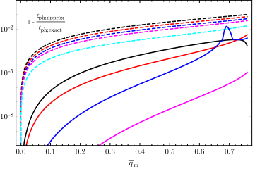
Figure 2: We consider here the Bardeen BH Bardeen68 , with specific magnetic charge $0<\bar{q}_{\text{m}}\lesssim 0.77$, and show the absolute relative error in estimating the exact value of its unstable circular photon-orbit impact parameter $\xi_{\text{ps;exact}}$ within the Carson-Yagi parametrization scheme (in dashed lines), which uses Taylor expansions to characterize metric functions, and in our scheme, which uses expansions of Padé approximants. Considering $\alpha_{13}$ to be the first non-trivial parameter of the CY approximation scheme, lines in the same color correspond to the same number of approximation parameters. To be clear, dashed-black and solid-black correspond to the $\alpha_{1i>13}=0$ Carson-Yagi and $a_{i>2}=0$ Padé approximation respectively. We also show in dashed-cyan the seventh-order CY relative error, i.e., for $\alpha_{1i>19}=0$. It is apparent that the Padé approximation does better already at first-order relative to the seventh-order Taylor expansion. Note also that the rapidity of convergence is much higher when employing Padé approximants.

Appendix B Comaprison with the Carson-Yagi Parametrisation Scheme

The metric of a spherically symmetric ($S=0$) BH spacetime in the Carson-Yagi (CY) parametrization scheme Carson_Yagi20 can be expressed as,

$$\text{d}s^{2}=-\left(1-\frac{2M}{r}\right)A_{1}^{-2}(r)~{}\text{d}t^{2}+\left(1-\frac{2M}{r}\right)^{-1}A_{5}^{-1}(r)~{}\text{d}r^{2}+r^{2}\text{d}\Omega_{2}^{2}\,,$$ (51)

where the functions $A_{1}(r)$ and $A_{5}(r)$ measure the deviation of an arbitrary BH metric from Schwarzschild. An asymptotic Taylor expansion for these functions is then employed to characterize them as,

$$A_{i}(r)=1+\sum_{n=1}^{\infty}\alpha_{i0}\left(\frac{M}{r}\right)^{n}\,.$$ (52)

To compare the rapidity of convergence of this scheme against the one used in the current work, we study the Bardeen-BH spacetime Bardeen68 . For this BH, we obtain the CY functions, $A_{1}$ and $A_{5}$, from Table 1 to be,

$$A_{1}(\bar{r})= \ \left(1-\frac{2}{\bar{r}}\right)^{1/2}\left(1-\frac{2\bar{r}^{2}}{\left(\bar{r}^{2}+\bar{q}_{\text{m}}^{2}\right)^{3/2}}\right)^{-1/2}\,,$$ (53)

$$A_{5}(\bar{r})= \ \left(1-\frac{2}{\bar{r}}\right)^{-1}\left(1-\frac{2\bar{r}^{2}}{\left(\bar{r}^{2}+\bar{q}_{\text{m}}^{2}\right)^{3/2}}\right)\,,$$ (54)

where in the above we have introduced $\bar{r}=r/M$ for brevity. Also, the parameter $\bar{q}_{\text{m}}$ corresponds to the parameter $g/M$ of Carson_Yagi20 . We obtain now the CY coefficients $\alpha_{i0}$ up to fifth order for this spacetime as,

$$\alpha_{10}= \ 1,\ \alpha_{13}=-\frac{3\bar{q}_{\text{m}}^{2}}{2},\ \alpha_{14}=-3\bar{q}_{\text{m}}^{2},\ \alpha_{15}=-6\bar{q}_{\text{m}}^{2}+\frac{15\bar{q}_{\text{m}}^{4}}{8}\,,$$

$$\alpha_{50}= \ 1,\ \alpha_{53}=3\bar{q}_{\text{m}}^{2},\ \alpha_{54}=6\bar{q}_{\text{m}}^{2},\ \alpha_{55}=12\bar{q}_{\text{m}}^{2}-\frac{15\bar{q}_{\text{m}}^{4}}{8}\,,$$ (55)

which can be verified to match the expressions in table 1 of Carson_Yagi20 . From the form of the functions in equation (53), it is clear that for appreciable specific magnetic charges $0\lnsim\bar{q}_{\text{m}}$, close to the horizon, which lies between $1.23\lesssim\bar{r}_{\text{H}}\lesssim 1.99$, arbitrarily high-order coefficients might become important in this parametrization scheme. We demonstrate this by showing in figure 2 how the impact parameter of a photon on the unstable circular geodesic in this spacetime, which is a near-horizon observable, is approximated within both the CY parametrization scheme and in our scheme.

Table 4: Here we show the relative error in approximating the first and second derivatives of the metric functions for all of the BH and non-BH spacetimes considered here.

Spacetime	Physical	Maximum relative error
	Charge	$dN/dx$	$d^{2}N/dx^{2}$	$dB/dx$	$d^{2}B/dx^{2}$
RN	$\bar{q}=0.5$	0	0	0	0
	$\bar{q}=0.9$	0	0	0	0
E-ae 2	[0.1, 0.1]	0	0	0	0
[$c_{13},c_{14}$]	[0.1, 0.9]	0	0	0	0
	[0.9, 1.7]	0	0	0	0
E-ae 1	$c_{13}=0.5$	0	0	0	0
	$c_{13}=0.9$	0	0	0	0
Bardeen	$\bar{q}_{\text{m}}=0.25$	0	3.04 [-9]	0	0
	$\bar{q}_{\text{m}}=0.75$	2.10 [-5]	1.09 [-3]	0	0
Hayward	$\bar{l}=0.25$	8.25 [-7]	5.35 [-6]	0	0
	$\bar{l}=0.75$	3.39 [-4]	5.43 [-3]	0	0
Bronnikov	$\bar{q}_{\text{m}}=0.5$	0	0	0	0
	$\bar{q}_{\text{m}}=1.05$	2.74 [-7]	7.17 [-6]	0	0
EEH	[1, 0.05]	1.96 [-5]	3.93 [-2]	0	0
[$\bar{q}_{\text{m}},\bar{\alpha}$]	[1, 1]	1.31 [-4]	4.75 [-2]	0	0
Frolov	[0.5, 0.25]	1.60 [-6]	1.22 [-5]	0	0
[$\bar{q},\bar{l}$]	[0.5, 0.6]	2.16 [-4]	3.76 [-3]	0	0
	[0.9, 0.25]	3.59 [-5]	9.83 [-4]	0	0
KS	$\bar{a}=1$	4.60 [-7]	2.93 [-6]	0	0
	$\bar{a}=10$	3.80 [-2]	6.93 [-2]	0	0
CFM A	$\beta=-0.9$	0	0	2.03 [-3]	2.01 [-2]
	$\beta=0.9$	0	0	2.65 [-6]	1.74 [-5]
CFM B	$\beta=1.1$	0	0	4.46 [-5]	7.7 [-5]
	$\beta=1.2$	0	0	7.26 [-3]	4.04 [-3]
Mod. Hayward	$\bar{l}=0.25$	8.25 [-7]	5.35 [-6]	9.96 [-2]	1.94 [-1]
	$\bar{l}=0.75$	3.39 [-4]	5.43 [-3]	9.20 [-2]	1.69 [-1]
EMd	$\bar{q}=0.7$	0	0	1.43 [-6]	1.32 [-6]
	$\bar{q}=1.4$	1.74 [-2]	4.29 [-2]	3.09 [-2]	6.58 [-2]
MBS A	-	4.79 [-2]	1.92 [-2]	8.06 [-2]	3.68 [-2]
MBS B	-	1.88 [-1]	2.94 [-1]	2.22 [-1]	5.08 [-1]
JNW	$\nu=0.1$	1.45 [-2]	3.55 [-2]	4.04 [-1]	2.60 [-2]
	$\nu=0.5$	4.31 [-3]	2.51 [-1]	1.02 [-2]	2.91 [-3]
	$\nu=0.9$	1.61 [-3]	1.31 [-2]	5.27 [-2]	2.63 [-2]

Table 5: Here we demonstrate the rapidity of convergence of the parametrization scheme used here by estimating the relative error in obtaining the unstable circular null geodesic impact factor $\xi_{\text{ps}}$ and ISCO frequency $\Omega_{{}_{\text{ISCO}}}$ at order-two and -four in the current parametrization scheme. We have omitted below those spacetimes for which the only relevant metric function $N$ for these observables is already exactly recovered at a lower order.

Spacetime	Physical	Maximum relative error
	Charge	$\xi_{\text{ps}}$		$\Omega_{{}_{\text{ISCO}}}$
		$a_{3}=0$	$a_{5}=0$	$a_{3}=0$	$a_{5}=0$
Bardeen	$\bar{q}_{\text{m}}=0.25$	3.71 [-6]	0	2.00 [-6]	1.49 [-9]
	$\bar{q}_{\text{m}}=0.75$	3.10 [-3]	7.35 [-6]	6.74 [-3]	2.21 [-5]
Hayward	$\bar{l}=0.25$	1.78 [-5]	1.20 [-7]	3.28 [-6]	2.56 [-6]
	$\bar{l}=0.75$	5.44 [-2]	1.29 [-4]	1.02 [-1]	2.26 [-4]
Bronnikov	$\bar{q}_{\text{m}}=0.5$	$\times$	$\times$	0	0
	$\bar{q}_{\text{m}}=1.05$	$\times$	$\times$	1.22 [-3]	2.95 [-8]
EEH	[1, 0.05]	$\times$	$\times$	8.31 [-4]	4.44 [-7]
[$\bar{q}_{\text{m}},\bar{\alpha}$]	[1, 1]	$\times$	$\times$	4.68 [-3]	2.22 [-4]
Frolov	[0.5, 0.25]	4.18 [-5]	2.66 [-7]	2.09 [-5]	4.37 [-6]
[$\bar{q},\bar{l}$]	[0.5, 0.6]	1.17 [-1]	7.87 [-5]	5.66 [-1]	1.59 [-4]
	[0.9, 0.25]	1.10 [-2]	1.47 [-5]	2.12 [-1]	3.80 [-6]
KS	$\bar{a}=1$	9.31 [-6]	6.66 [-8]	1.39 [-6]	1.45 [-6]
	$\bar{a}=10$	2.78 [-2]	8.62 [-3]	1.11 [-1]	4.34 [-2]
Mod. Hayward	$\bar{l}=0.25$	5.44 [-2]	1.29 [-4]	1.02 [-1]	2.26 [-4]
	$\bar{l}=0.75$	1.78 [-5]	1.20 [-7]	3.28 [-6]	2.56 [-6]
EMd	$\bar{q}=0.7$	4.43 [-7]	0	3.97 [-7]	0
	$\bar{q}=1.4$	7.62 [-1]	7.22 [-3]	2.93 [-1]	6.84 [-3]
MBS A	-	$\times$	$\times$	$\times$	$\times$
MBS B	-	$\times$	$\times$	$\times$	$\times$
JNW	$\nu=0.1$	$\times$	$\times$	$\times$	$\times$
	$\nu=0.5$	$\times$	$\times$	3.54 [-3]	7.81 [-3]
	$\nu=0.9$	2.86 [-3]	6.95 [-4]	7.85 [-3]	1.11 [-3]

Appendix C Goodness of Approximation and Convergence Tests

The fourth-order approximations of the metric functions for the various spacetimes under consideration here are smooth throughout the range of the conformal coordinate $0\!\leq x\!<\!1$. To demonstrate the accuracy in obtaining the metric function up to two derivatives, we report the relative errors in approximating them in table 4, which are typically appreciably low.

We also demonstrate the rapidity of the order-on-order convergence of our parametrization scheme by estimating the relative error in obtaining the unstable circular null geodesic impact factor $\xi_{\text{ps}}$ and ISCO frequency $\Omega_{{}_{\text{ISCO}}}$ at the second and fourth order in Padé expansion. This is reported in table 5. We gain about two orders of accuracy by going two orders higher in the Padé expansion.