Higher Form Symmetries of Argyres-Douglas Theories

Abstract

We determine the structure of 1-form symmetries for all 4d $\mathcal{N}=2$ theories that have a geometric engineering in terms of type IIB string theory on isolated hypersurface singularities. This is a large class of models, that includes Argyres-Douglas theories and many others. Despite the lack of known gauge theory descriptions for most such theories, we find that the spectrum of 1-form symmetries can be obtained via a careful analysis of the non-commutative behaviour of RR fluxes at infinity in the IIB setup. The final result admits a very compact field theoretical reformulation in terms of the BPS quiver. We illustrate our methods in detail in the case of the $(\mathfrak{g},\mathfrak{g}^{\prime})$ Argyres-Douglas theories found by Cecotti-Neitzke-Vafa. In those cases where $\mathcal{N}=1$ gauge theory descriptions have been proposed for theories within this class, we find agreement between the 1-form symmetries of such $\mathcal{N}=1$ Lagrangian flows and those of the actual Argyres-Douglas fixed points, thus giving a consistency check for these proposals.

1 Introduction

Four-dimensional supersymmetric quantum field theories are an ideal laboratory to probe our understanding of strongly coupled relativistic systems. In this context, $\mathcal{N}=2$ supersymmetric models are particularly useful since they have enough supercharges to constrain the perturbative corrections while still allowing for interesting dynamics. In the past two decades a wide variety of new $\mathcal{N}=2$ theories have been constructed exploiting various kinds of geometric engineering techniques in string theory — for a nice review see Tachikawa:2013kta . There is no known Lagrangian description for many of the $\mathcal{N}=2$ theories so obtained, which makes it essential to develop techniques to study these theories that are independent from a Lagrangian formulation. A natural basic question in this context is to determine all the symmetries for these models, including the higher symmetries Gaiotto:2014kfa . In this paper we take a first step in this direction, and determine the 1-form symmetries of a broad class of $\mathcal{N}=2$ theories in four dimensions, namely those that arise from IIB on hypersurface singularities. Many well known $\mathcal{N}=2$ theories belong to this class, and we will analyse the details of a number of examples below.

One generic feature of the theories that we study is that non-local BPS dyons become simultaneously massless. The original examples of this phenomenon were given by Argyres and Douglas in Argyres:1995jj ; Argyres:1995xn . Since the massless degrees of freedom are mutually non-local, the corresponding dynamics cannot be described by a conventional Lagrangian. Moreover, by the scale invariance of the corresponding Seiberg-Witten (SW) geometry, the theories are argued to be $\mathcal{N}=2$ superconformal.

Argyres-Douglas theories can be realized in Type IIB superstrings on isolated hypersurface singularities Eguchi:1996vu ; Eguchi:1996ds . This perspective allows to compute the corresponding spectrum of BPS states from the bound states of D3 branes on vanishing special Lagrangian 3-cycles Shapere:1999xr . The same geometric construction can be generalized to more general hypersurface singularities at finite distance in moduli space — which translates to the requirement that the corresponding 2d (2,2) Landau-Ginzburg worldsheet theory has central charge $\hat{c}<2$ Gukov:1999ya ; Shapere:1999xr . Each such model is characterized by a quasihomogeneous polynomial

$$f(\lambda^{w_{i}}X_{i})=\lambda^{d}f(X_{i})$$ (1)

where $d$ and $w_{i}$ are positive integers known respectively as degree and weights of the singularity, and the corresponding geometry is given by $\mathbf{X}_{6}\coloneqq\{f(X_{i})=0\}$. The $\mathbb{C}^{*}$ action in (1) plays the same role of the scale invariance for the SW geometry: it is well-known that this can be exploited to compute the dimensions of the various Coulomb branch operators of the SCFT Shapere:1999xr . These singularities are at finite distance in moduli space provided $\sum_{i}w_{i}>d$ which is the singularity theory translation of the condition $\hat{c}<2$ Vafa:1988uu ; Lerche:1989uy .

The interesting part of the defect group for theories of this class is given by

$$\mathbb{D}^{(1)}=\mathbb{Z}^{\kappa}\,\oplus{\bigoplus}_{i=1}^{n}\Big{(}\mathbb{Z}_{m_{i}}\oplus\mathbb{Z}_{m_{i}}\Big{)}$$ (3)

where $n$ is the rank of the SCFT and $\kappa$ is the rank of its flavor symmetry group. The $m_{i}$’s are positive integers that we determine below — if for some $i$ the corresponding $m_{i}$ equals 1, the corresponding factor is trivial and the summand is dropped above. The torsional groups in parenthesis are non-trivially paired, meaning that the corresponding charge operators form a non-commuting Heisenberg algebra.

Notice that in the formulas above, we include the free factors of the defect group. We stress here that to each free $\mathbb{Z}$ factor in the $j$-form defect group $\mathbb{D}^{(j)}$ there is a corresponding abelian $U(1)$ higher form symmetry which is shifted in degree by one. For instance, the free factor of $\mathbb{D}^{(1)}$ in equation (3) corresponds to the continuous zero-form symmetries of these SCFTs. For such zero-form symmetries this group can enhance to become non-Abelian — see Caorsi:2018ahl ; Caorsi:2019vex for conditions about the enhancement of the flavor symmetries in terms of the corresponding categories of BPS states. It is also interesting to remark that in the language of those papers, the Grothendieck group of the cluster category associated to the BPS quiver precisely coincides with the full $\mathbb{D}^{(1)}$ we compute in this paper, referred to as the ’t Hooft group in CDZ ; Caorsi:2016ebt — see §2.3 below.

Exploiting the Milnor-Orlik conjecture OM , and its subsequent proof by Boyer, Galicki and Simanca for the case of interest in this paper Boyer , we can rewrite (3) as follows:

$$\mathbb{D}^{(1)}=\mathbb{Z}^{\kappa}\oplus\bigoplus_{i=1}^{4}\mathbb{Z}_{r_{i}}^{2g_{i}}$$ (4)

In terms of singularity theory data, we have that $\kappa$ is given by sasakianBIBLE

$$\kappa=\sum(-1)^{4-s}{u_{i_{1}}\cdots u_{i_{s}}\over v_{i_{1}}\cdots v_{i_{s}}\,\text{lcm}(u_{i_{1}}\cdots u_{i_{s}})}$$ (5)

where

$$u_{i}={d\over\text{gcd}(d,w_{i})}\qquad v_{i}={w_{i}\over\text{gcd}(d,w_{i})}$$ (6)

and the sum is taken over all the 16 subsets $\{i_{1},...,i_{s}\}$ with $s$ elements of the index set $\{1,2,3,4\}$. Moreover,

$$r_{i}=\text{gcd}(w_{1},..,\hat{w}_{i},...,w_{4})$$ (7)

and

$$2g_{i}=-1+\sum_{j\neq i}\frac{\text{gcd}(d,w_{j})}{w_{j}}-d\sum_{j<k\atop j,k\neq i}\frac{\text{gcd}(w_{j},w_{k})}{w_{j}w_{k}}+d^{2}\frac{r_{i}}{w_{1}...\hat{w}_{i}...w_{4}}\,,$$ (8)

where the notation $\hat{w}$ means that $w$ is omitted.

Within the class of theories engineered by type IIB superstrings on hypersurface singularities, a subset of geometries that naturally generalizes the original examples by Argyres and Douglas are the Cecotti-Neitzke-Vafa $(\mathfrak{g},\mathfrak{g}^{\prime})$ SCFTs, or $\mathcal{T}[\mathfrak{g},\mathfrak{g}^{\prime}]$ for short Cecotti:2010fi . These are also known as the generalized Argyres-Douglas theories of type $(\mathfrak{g},\mathfrak{g}^{\prime})$ Xie:2012hs . Consider a background of the form $\mathcal{M}_{4}\times\mathbf{X}_{6}$, where $\mathcal{M}_{4}$ is some arbitrary closed four-manifold, which we will always assume to be closed $\mathrm{Spin}$ without torsion, and $\mathbf{X}_{6}$ is a non-compact Calabi-Yau threefold with an isolated singularity, given by the hypersurface

$$P_{(\mathfrak{g},\mathfrak{g}^{\prime})}(x,y,w,z)=P_{\mathfrak{g}}(x,y)+P_{\mathfrak{g}^{\prime}}(w,z)=0$$ (9)

inside $\mathbb{C}^{4}$. Here

$$\begin{array}[]{c|c}\mathfrak{g}&P_{\mathfrak{g}}(x,y)\\ \hline\cr A_{n}&x^{2}+y^{n+1}\\ D_{n}&x^{2}y+y^{n-1}\\ E_{6}&x^{3}+y^{4}\\ E_{7}&x^{3}+xy^{3}\\ E_{8}&x^{3}+y^{5}\end{array}$$ (10)

are such that $z^{2}+P_{\mathfrak{g}}(x,y)=0$ is the du Val singularity of type $\mathfrak{g}$. This space has an isolated singularity at $x=y=z=w=0$. The corresponding 2d $(2,2)$ LG theory has superpotential $W=P_{(\mathfrak{g},\mathfrak{g}^{\prime})}(x,y,w,z)$. The resulting 2d worldsheet theory has central charge $\hat{c}<2$ in this case Cecotti:2010fi , and these singularities are at finite distance. It is believed that at low energies this configuration can be described by the $\mathcal{T}[\mathfrak{g},\mathfrak{g}^{\prime}]$ four dimensional SCFT compactified on $\mathcal{M}_{4}$. The non-trivial local degrees of freedom of such SCFT arise from massless D3 branes wrapped on the vanishing three-cycles at the singular point of $\mathbf{X}_{6}$.

The local degrees of freedom of $\mathcal{T}[\mathfrak{g},\mathfrak{g}^{\prime}]$ are in this way fully determined by the choice of geometry, but in presence of a nontrivial defect group at the horizon of the IIB compactification, extra information is required to fully specify the theory and its partition function on $\mathcal{M}_{4}$ Garcia-Etxebarria:2019cnb — see also DelZotto:2015isa ; Albertini:2020mdx ; Morrison:2020ool . The most well known example of this fact is the case of the $\mathcal{N}=4$ theory with simple ADE algebra $\mathfrak{g}$ corresponding to IIB on $\mathbb{T}^{2}\times\mathbb{C}^{2}/\Gamma_{\mathfrak{g}}$. While giving $\Gamma_{\mathfrak{g}}$ fully specifies the spectrum of local operators (and their correlators), in order to compute the partition function on topologically non-trivial manifolds we need to specify additional data, fixing the global structure of the theory and, in particular, its 1-form symmetries. Our main result in this paper is to determine the defect group for the geometries associated to the $\mathcal{T}[\mathfrak{g},\mathfrak{g}^{\prime}]$ theories, and the corresponding Heisenberg algebra of noncommuting fluxes. We find that many of these theories admit different inequivalent global structures and hence distinct partition functions on four-manifolds with nontrivial intersecting 2-cycles. While this does not affect the superconformal index for these models Buican:2015ina ; Cordova:2015nma ; Cordova:2016uwk ; Buican:2015tda ; Cecotti:2015lab ; Xie:2016evu ; Xie:2019zlb which corresponds to the partition function on $S^{1}\times S^{3}$, it does affect the lens space index or more complicated partition functions (see e.g. Razamat:2013jxa ; Razamat:2014pta ; Festuccia:2016gul ; Festuccia:2018rew for some interesting examples of $\mathcal{N}=2$ backgrounds that would be interesting to couple to AD SCFTs).

As there are no known Lagrangian descriptions of most $\mathcal{T}[\mathfrak{g},\mathfrak{g}^{\prime}]$ SCFTs (with the exception of some cases; we will come back to these momentarily) it might seem hard to find the 1-form symmetries for these theories using purely field theoretical tools. However, as we explain below — extending previous results DelZotto:2015isa ; Garcia-Etxebarria:2019cnb ; Morrison:2020ool ; Albertini:2020mdx to the four dimensional setting — there is a way of rephrasing the results from the IIB analysis in purely field theoretical terms. We find that the role played by the unscreened part of the center of the gauge group in the analysis in Aharony:2013hda is played in the non-Lagrangian setting in this paper by $\operatorname{Tor}(\operatorname{coker}\mathsf{Q})$, with $\mathsf{Q}$ the BPS quiver for the theory Cecotti:2011rv ; Alim:2011kw . The free part of the group $\operatorname{coker}\mathsf{Q}$ coincides with the factor $\mathbb{Z}^{\kappa}$, hence $\mathbb{D}^{(1)}=\operatorname{coker}\mathsf{Q}$: it is natural to expect that this field theoretical formulation will be general, even in the absence of a simple IIB construction, and indeed this follows from the analysis done in Caorsi:2016ebt ; we will explore this point further in upcoming work ADZGEH .

The results in this paper can be used to provide a subtle but powerful test of any proposed Lagrangian dual description of the $\mathcal{T}[\mathfrak{g},\mathfrak{g}^{\prime}]$ theories, imposing matching of 1-form symmetries. Such Lagrangian descriptions have in fact been recently proposed by Maruyoshi:2016aim ; Maruyoshi:2016tqk ; Agarwal:2017roi (see also Benvenuti:2017bpg ; Giacomelli:2017ckh ; Carta:2020plx ), in terms of $\mathcal{N}=2$ theories perturbed by $\mathcal{N}=1$ relevant deformations. We find that the Lagrangians proposed in the literature have precisely the same structure of 1-form symmetries as the $\mathcal{T}[\mathfrak{g},\mathfrak{g}^{\prime}]$ theories to which they are believed to flow. Our computations also provide interesting additional constraints on the existence of potential Lagrangian descriptions for those theories for which no Lagrangians are known.

The structure of this paper is as follows. In section 2 we review the results of Garcia-Etxebarria:2019cnb ; Albertini:2020mdx that are needed for our analysis, as well as some aspects of the geometric engineering of IIB string theory on hypersurface singularities. In section 3 the main result of the paper is derived (our readers interested mainly in the result of the analysis can skip to table 1), and we explain how our results are consistent with the $\mathcal{N}=1$ Lagrangian flows proposed in Maruyoshi:2016aim ; Maruyoshi:2016tqk ; Agarwal:2017roi . A computation in K-theory necessary to justify our mathematical description of the defect groups is presented in the appendix.

Note added: while this work was reaching completion, we received SAKURA2 that has a small overlap with some of our results. We thank the authors of that paper to accept coordinating the submission of our papers to the arXiv.

2 Geometric engineering and higher symmetries

In this section we review how to compute the spectrum of higher form symmetries for geometrically engineered $\mathcal{N}=2$ theories. We refer the reader to Garcia-Etxebarria:2019cnb for a more in-depth discussion, here we will just highlight the modifications necessary when dealing with Calabi-Yau threefolds.

2.1 Global structure and flux non-commutativity

Consider IIB superstring theory on

$$\mathcal{M}_{4}\times\mathbf{X}_{6}\,,$$ (11)

where $\mathbf{X}_{6}$ is a local Calabi-Yau threefold. Via geometric engineering, this computes the partition function of a 4d $\mathcal{N}=2$ theory

$${\mathcal{T}}_{\mathbf{X}_{6}}\in\text{SQFT}_{3+1}^{\,\mathcal{N}=2}$$ (12)

coupled to a four-manifold $\mathcal{M}_{4}$. In what follows we will denote such partition function $Z_{{\mathcal{T}}_{\mathbf{X}_{6}}}(\mathcal{M}_{4})$. Notice that ${\mathcal{T}}_{\mathbf{X}_{6}}$ is not necessarily conformal: for instance, if one considers the IIB geometry

$$\mathbf{X}_{6}\equiv\Big{\{}e^{z}+e^{-z}+p_{\mathfrak{g}}(x,y)+u^{2}=0\Big{\}}\,\subset\mathbb{C}^{4}\,,$$ (13)

the corresponding ${\mathcal{T}}_{\mathbf{X}_{6}}$ is the $\mathcal{N}=2$ supersymmetric Yang-Mills (SYM) theory with simple simply-laced gauge algebra $\mathfrak{g}$. The partition function $Z_{{\mathcal{T}}_{\mathbf{X}_{6}}}(\mathcal{M}_{4})$ should be fully determined by the data of the string background. This is indeed true, but in the case that ${\mathcal{T}}_{\mathbf{X}_{6}}$ has non-trivial higher symmetries there are important subtleties.

The higher $n$-form symmetries in the four dimensional theory act on the $n$-dimensional defects of the theory. In geometric engineering these defects arise from D$p$-branes wrapping $k$-cycles on $\mathbf{X}_{6}$, where $n=p-k+1\leq 4$. More concretely, any background for the higher form symmetries introduces monodromies for these defects, so in the string theory construction such a background must be realized with a choice of background fluxes. The latter are then providing the stringy realization of higher form symmetries. Therefore, in order to fully specify the theory ${\mathcal{T}}_{\mathbf{X}_{6}}$, we need to specify the fluxes on the IIB construction.

It is natural to ask at this point whether there is any canonical choice for the RR background fluxes. For instance, if we could just set the flux to zero this would give a canonical choice of ${\mathcal{T}}_{\mathbf{X}_{6}}$ for each geometry $\mathbf{X}_{6}$. Since $\mathbf{X}_{6}$ is a local CY, we must in particular be aware of the behavior of the flux at infinity. It turns out that generically no canonical choice of “zero flux” at infinity exists, rather we have an obstruction which can be argued for as follows. For any field theory in $d+1$ spacetime dimensions, to each codimension one submanifold $\mathcal{N}_{d}$ of spacetime we assign a Hilbert space $\mathcal{H}(\mathcal{N}_{d})$, the space of possible field configurations that are allowed in the quantum theory on that spatial slice. We obtain this Hilbert space by quantizing the Hamiltonian of the theory on $\mathbb{R}\times\mathcal{N}_{d}$, where we treat the first coordinate as the time direction. Similarly, when we consider a string compactification on a manifold with boundary, we obtain a Hilbert space. In order to understand which field configurations can be put at infinity, we need to understand the Hilbert space that type IIB string theory associates to the boundary $\mathcal{N}_{9}\coloneqq\mathcal{M}_{4}\times Y_{5}$. Luckily, for our purposes a rather coarse understanding of this Hilbert space will be enough, and in particular we will only need to understand its grading by fluxes.

Our Calabi-Yau threefold $\mathbf{X}_{6}$ is a cone over some Sasaki-Einstein space $Y_{5}$, so the choice of boundary conditions at infinity can be understood as the limiting behaviour of a family of field configurations at constant radius $r$ in the cone, as $r\to\infty$. The topology of each slice is $\mathcal{M}_{4}\times Y_{5}$, so the problem is to understand which choices of field configurations can we put on $\mathcal{M}_{4}\times Y_{5}$ slices of spacetime.

The relevant grading of Hilbert space was understood by Freed, Moore and Segal in Freed:2006yc ; Freed:2006ya . They showed that whenever $\mathcal{N}_{9}$ has torsion, the operators measuring flux expectation values become non-commutative. More precisely, the operators measuring electric flux do not commute with the operators measuring magnetic flux. The $F_{5}$ flux is self-dual, so in this case the flux operators for $F_{5}$ do not commute among themselves. The precise commutation relation for $F_{5}$ fluxes is as follows. To each cohomology class $\sigma\in\operatorname{Tor}H^{5}(\mathcal{N}_{9})$ we associate an operator $\Phi_{\sigma}$, which measures the torsional part of the flux on a four-cycle in $\mathcal{N}_{9}$ Poincaré dual to $\sigma$. In the usual (but somewhat imprecise in the current context) differential form language, these operators would be of the form $\Phi_{\sigma}=\exp(i\int_{\mathcal{N}_{9}}A_{\sigma}\wedge F_{5})$ where $A_{\sigma}$ is a flat connection for the torsional class $\sigma$.

The commutation relations between these operators are then

$$\Phi_{\sigma}\Phi_{\sigma^{\prime}}=e^{2\pi i\,\mathsf{L}(\sigma,\sigma^{\prime})}\Phi_{\sigma^{\prime}}\Phi_{\sigma}$$ (14)

with $\mathsf{L}(\sigma,\sigma^{\prime})\colon\operatorname{Tor}H^{5}(\mathcal{N}_{9})\times\operatorname{Tor}H^{5}(\mathcal{N}_{9})\to\mathbb{Q}/\mathbb{Z}$ the linking number between the cohomology classes (we will discuss this linking number in more detail below). We refer the reader to the original papers Freed:2006yc ; Freed:2006ya for a derivation of these commutation relations. At any rate, what this implies for the grading of Hilbert space $\mathcal{H}(\mathcal{N}_{9})$ by fluxes, and thus for the available choices of boundary conditions, is that there is no zero flux eigenstate $\left|\bf 0\right\rangle$ such that $\Phi_{\sigma}\left|\bf 0\right\rangle=\left|\bf 0\right\rangle$ for all $\sigma\in\operatorname{Tor}(H^{5}(\mathcal{N}_{9}))$.

The best that we can do when choosing boundary conditions is to choose a maximally commuting set $L$ of operators, and impose that our boundary state is neutral under these. In detail, we define $s(\sigma,\sigma^{\prime})\coloneqq e^{2\pi i\,\mathsf{L}(\sigma,\sigma^{\prime})}$, and define a maximal isotropic subgroup $L\subset\operatorname{Tor}H^{5}(\mathcal{N}_{9})$ to be a maximal set such that $s(\sigma,\sigma^{\prime})=1$ for all $\sigma,\sigma^{\prime}\in L$. This implies that the subgroup generated by the operators $\{\Phi_{\sigma}|\sigma\in L\}$ is abelian, and provides a maximal set of commuting observables. Once we choose $L$, there is a unique state $\left|{\bf 0};L\right\rangle$ in the Hilbert space $\mathcal{H}(\mathcal{N}_{9})$ such that $\Phi_{\sigma}\left|{\bf 0};L\right\rangle=\left|{\bf 0};L\right\rangle$ for all $\sigma\in L$. We can interpret this state as follows. Define

$$F_{L}\coloneqq\frac{\operatorname{Tor}H^{5}(\mathcal{N}_{9})}{L}$$ (15)

and choose a representative $\mathbf{f}$ of each coset. Then the states $\left|\mathbf{f};L\right\rangle\coloneqq\Phi_{\mathbf{f}}\left|\mathbf{0};L\right\rangle$ are eigenvectors of the flux operators in $L$:

$$\Phi_{\sigma}\left|\mathbf{f};L\right\rangle=s(\sigma,\mathbf{f})\left|\mathbf{f};L\right\rangle\,,$$ (16)

so we find that the $\left|\mathbf{f};L\right\rangle$ are the states with definite flux in $L$. In particular, $\left|\mathbf{0};L\right\rangle$ can be interpreted as a state with zero flux in $L$. Once $L$ is chosen this state is unique, so the non-canonical nature of the choice of boundary condition reduces to the absence of a canonical choice for $L$ in $H^{5}(\mathcal{N}_{9})$.

In this paper we focus on the case $\mathcal{N}_{9}=\mathcal{M}_{4}\times Y_{5}$, with $\operatorname{Tor}H^{\bullet}(\mathcal{M}_{4})=0$ so by the Künneth formula we have

$$\operatorname{Tor}H^{5}(\mathcal{N}_{9})=\bigoplus_{n=0}^{4}H^{n}(\mathcal{M}_{4})\otimes\operatorname{Tor}H^{5-n}(Y_{5})\,.$$ (17)

In the cases of interest to us we additionally have that $Y_{5}$ is simply connected 10.2307/j.ctt1bd6kvv , so $\operatorname{Tor}H_{1}(Y_{5})=\operatorname{Tor}H^{4}(Y_{5})=0$. The universal coefficient theorem Hatcher:478079 additionally implies that $\operatorname{Tor}H^{2}(Y_{5})=\operatorname{Tor}H_{1}(Y_{5})=0$, so the only possible non-trivial torsion lives in $H^{3}(Y_{5})$:

$$\operatorname{Tor}H^{5}(\mathcal{N}_{9})=H^{2}(\mathcal{M}_{4})\otimes\operatorname{Tor}H^{3}(Y_{5})\cong H^{2}(\mathcal{M}_{4};\operatorname{Tor}H^{3}(Y_{5}))\,.$$ (18)

In principle we should now classify all the $L\subset\operatorname{Tor}H^{5}(\mathcal{N}_{9})$ for every $\mathcal{N}_{9}$, but there is a class of such isotropic subgroups which is particularly interesting in the context of four dimensional physics on $\mathcal{M}_{4}$. Assume that we fix a $Y_{5}$, or equivalently its cone $X_{6}$. Then there is a subclass of the possible $L$ of the form

$$L=L_{5}\otimes H^{2}(\mathcal{M}_{4})$$ (19)

that can be defined uniformly for every $\mathcal{M}_{4}$. Here $L_{5}$ is a maximal isotropic subgroup of $\operatorname{Tor}H^{3}(Y_{5})$. The theories defined by such choices are sometimes called “genuine” four dimensional theories.

The choices of global structure for the genuine ${\mathcal{T}}_{\mathbf{X}_{6}}$ theories are thus the choices of maximal isotropic $L_{5}\subset\operatorname{Tor}H^{3}(Y_{5})$, with $\partial\mathbf{X}_{6}=Y_{5}$. Once we have such an $L_{5}$ we have a choice for the 2-surface operators generating the 1-form symmetries of ${\mathcal{T}}_{\mathbf{X}_{6}}$: they come from the reduction of the $\Phi_{\sigma}$ flux operators in the IIB theory. And relatedly, introducing background fluxes for $F_{5}$ at infinity will introduce background fluxes for the 1-form symmetries in the four-dimensional theory on $\mathcal{M}_{4}$.

2.2 The case of hypersurface singularities

Our discussion so far has been fairly general, and has not required us to make use of the fact that the ${\mathcal{T}}_{\mathbf{X}_{6}}$ theories preserve $\mathcal{N}=2$. In fact, in addition to being $\mathcal{N}=2$ supersymmetric the theories that we will be discussing have the nice property that their BPS spectrum can be generated from a BPS quiver Cecotti:2011rv ; Alim:2011kw (we refer the reader unfamiliar with BPS quivers to these papers for reviews), and this leads to a reformulation of the answer that we just found in terms of screening of line operators, generalizing to our current context the discussions in Aharony:2013hda ; DelZotto:2015isa .

Recall that each node in the BPS quiver represents a BPS building block, and the arrows encode how they can be recombined. From the IIB perspective, the nodes in the quiver represent D3 branes wrapped on generators of a basis of $H_{3}(\mathbf{X}_{6})$, and the arrows in the quiver encode the intersection numbers of the corresponding 3-cycles. BPS states in ${\mathcal{T}}_{\mathbf{X}_{6}}$ can be obtained from D3 branes wrapping supersymmetric compact cycles in $\mathbf{X}_{6}$, and such D3 branes can always be constructed by taking a combination of generators with the right total charge, and recombining them.

We can connect our discussion in the previous section to the formulation in terms of BPS quivers as follows. Take a small 7-dimensional sphere $S^{7}$ around the origin in $\mathbb{C}^{4}$. Our “boundary at infinity” $Y_{5}$ is homotopy equivalent to the intersection $\mathcal{Y}_{5}=S^{7}\cap\{P_{(\mathfrak{g},\mathfrak{g}^{\prime})}=\epsilon\}$, where $P_{(\mathfrak{g},\mathfrak{g}^{\prime})}$ was the polynomial (9) defining the Argyres-Douglas theory, and we take $\epsilon$ small but non-vanishing in order to make the interior of $\mathcal{Y}_{5}$ smooth. Finally, introduce $\mathcal{X}_{6}$ to be the (smooth) interior of $\mathcal{Y}_{5}$, namely the intersection of a ball $B^{8}$ (such that $\partial B^{8}=S^{7}$) with $P_{(\mathfrak{g},\mathfrak{g}^{\prime})}=\epsilon$.

Since $\partial\mathcal{X}_{6}=\mathcal{Y}_{5}$ there is a long exact sequence in homology of the form

$$\ldots\to H_{n}(\mathcal{Y}_{5})\to H_{n}(\mathcal{X}_{6})\to H_{n}(\mathcal{X}_{6},\mathcal{Y}_{5})\to H_{n-1}(\mathcal{Y}_{5})\to\ldots$$ (20)

where $H_{n}(\mathcal{X}_{6},\mathcal{Y}_{5})$ denotes relative homology, and the maps in the same degree are the obvious ones.

We are interested in $\operatorname{Tor}H^{3}(\mathcal{Y}_{5})=\operatorname{Tor}H_{2}(\mathcal{Y}_{5})$. It is a classical result of Milnor (see theorems 5.11 and 6.5 of 10.2307/j.ctt1bd6kvv ) that $\mathcal{X}_{6}$ has the homotopy type of a bouquet of three-spheres, and in particular $H_{2}(\mathcal{X}_{6})=0$. The long exact sequence in homology above then implies that

$$H_{2}(\mathcal{Y}_{5})=\frac{H_{3}(\mathcal{X}_{6},\mathcal{Y}_{5})}{H_{3}(\mathcal{X}_{6})}$$ (21)

where the embedding of $H_{3}(\mathcal{X}_{6})$ into $H_{3}(\mathcal{X}_{6},Y_{5})$ is the natural one. This equation has a natural interpretation in terms of four dimensional field theory, as follows. The numerator denotes the homology class of 3-cycles in $\mathcal{X}_{6}$, including those that extend to the boundary. If we wrap D3 branes on these cycles we obtain lines in the four dimensional theory. The D3 branes wrapping compact 3-cycles in $\mathcal{X}_{6}$ give dynamical lines, while the ones extending to the boundary give line defects. The denominator includes the dynamical lines only, so (21) is saying that in order to understand the global structure of the theory, we need to consider the line defects modulo the dynamical excitations, or in other words the unscreened part of the line defect charge, as in Aharony:2013hda ; DelZotto:2015isa .

It is convenient to rephrase the previous discussion in the language of cohomology groups. Lefschetz duality implies that $H_{3}(\mathcal{X}_{6},\mathcal{Y}_{5})\cong H^{3}(\mathcal{X}_{6})$, and the universal coefficient theorem then implies that $H_{3}(\mathcal{X}_{6},\mathcal{Y}_{5})\cong\operatorname{Hom}(H_{3}(\mathcal{X}_{6}),\mathbb{Z})$. On the other hand, the embedding of $H_{3}(\mathcal{X}_{6})$ into $\operatorname{Hom}(H_{3}(\mathcal{X}_{6}),\mathbb{Z})$ is given simply by the partial evaluation of the intersection form $q\colon H_{3}(\mathcal{X}_{6})\times H_{3}(\mathcal{X}_{6})\to\mathbb{Z}$. That is, given any element $x\in H_{3}(\mathcal{X}_{6})$ we have an embedding $Q\colon H_{3}(\mathcal{X}_{6})\to\operatorname{Hom}(H_{3}(\mathcal{X}_{6}),\mathbb{Z})$ given by $Q(x)=q(x,\cdot)$. We can thus rewrite (21) as $H_{2}(\mathcal{Y}_{5})=\operatorname{coker}(q)$, or equivalently

$$H_{2}(\mathcal{Y}_{5})=\operatorname{coker}(Q)\,.$$ (22)

Now, $Q$ is an integer-valued antisymmetric matrix, so there is a change of basis to $\mathsf{Q}$ (that is, an integer matrix $P$ with $\det(P)=\pm 1$ such that $Q=P^{t}\mathsf{Q}P$) with (see theorem IV.1 in newman1972integral )

$$\mathsf{Q}=\begin{pmatrix}0&r_{1}\\ -r_{1}&0\\ &&0&r_{2}\\ &&-r_{2}&0\\ &&&&\ddots\\ &&&&&0&r_{n}\\ &&&&&-r_{n}&0\\ &&&&&&&0\quad\,\\ &&&&&&&&\ddots\\ &&&&&&&&&\quad 0\end{pmatrix}$$ (23)

and $r_{i}\in\mathbb{Z}$, such that $r_{i}\mid r_{i+1}$. Without loss of generality we can choose $r_{i}>0$. Since $P$ is invertible we have $\operatorname{coker}(Q)=\operatorname{coker}(\mathsf{Q})$. Let us focus on a single $2\times 2$ block in $\mathsf{Q}$ of the form

$$\mathsf{Q}_{i}=\begin{pmatrix}0&r_{i}\\ -r_{i}&0\end{pmatrix}$$ (24)

with $r_{i}>0$. We denote the generators of $H_{3}(\mathcal{X}_{6})$ on this subspace $a,b$, and the dual elements $a^{*},b^{*}\in\operatorname{Hom}(H_{3}(\mathcal{X}_{6}))$. We have $\mathsf{Q}_{i}(a)=r_{i}b^{*}$ and $\mathsf{Q}_{i}(b)=-r_{i}a^{*}$. This implies that $\operatorname{coker}(\mathsf{Q}_{i})=\mathbb{Z}_{r_{i}}\oplus\mathbb{Z}_{r_{i}}$. We thus have

$$\operatorname{coker}(\mathsf{Q})=\mathbb{Z}^{\kappa}\oplus\sum_{i=1}^{n}\mathbb{Z}_{r_{i}}\oplus\mathbb{Z}_{r_{i}}$$ (25)

with

$$\kappa=\operatorname{rk}(H_{3}(\mathcal{X}_{6}))-2n=\operatorname{rk}F$$

is the factor corresponding to the 0-form flavor symmetry of the theory, while $n$ is its rank (i.e. the dimension of the Coulomb branch of the SCFT). This determines $\operatorname{Tor}H_{2}(\mathcal{Y}_{5})$ as an abelian group

$$\operatorname{Tor}H_{2}(\mathcal{Y}_{5})=\sum_{r_{i}>1}\mathbb{Z}_{r_{i}}\oplus\mathbb{Z}_{r_{i}}\,.$$ (26)

The case $r_{i}=1$ is trivial; we choose to exclude it from the sum.

In order to understand the global structure of the Argyres-Douglas theories we need a final piece of additional information, the linking pairing between elements in $H_{2}(\mathcal{Y}_{5})$. Let us focus again on a single block $\mathsf{Q}_{i}$, with $r_{i}>1$. The linking form $\mathsf{L}_{i}$ on $[\operatorname{Tor}H_{2}(\mathcal{Y}_{5})]_{i}$ (that is, the $i$-th block of $\operatorname{Tor}H_{2}(\mathcal{Y}_{5})$) is related very simply to $\mathsf{Q}_{i}$ GordonLitherland :

$$\mathsf{L}_{i}=\mathsf{Q}_{i}^{-1}=\begin{pmatrix}0&-\frac{1}{r_{i}}\\ \frac{1}{r_{i}}&0\end{pmatrix}\mod 1\,.$$ (27)

The final answer from our analysis is thus quite straightforward. Recall from (19) that we are after maximal isotropic subgroups of $\operatorname{Tor}H_{2}(\mathcal{Y}_{5})$, where the commutation relations are determined by the linking form $\mathsf{L}$. From the form above, the problem then reduces to the classification of the maximal isotropic sublattices for each block of $\mathsf{Q}_{i}$, that is the maximal isotropic sublattices of $\mathbb{Z}_{r_{i}}\oplus\mathbb{Z}_{r_{i}}$ with the pairing (27). (This problem is isomorphic to the problem of determining the global forms of the $\mathcal{N}=4$ $\mathfrak{su}(r_{i})$ theory, studied in Aharony:2013hda .)

As an example, assume that

$$\mathsf{Q}=\begin{pmatrix}0&2\\ -2&0\\ &&0&2\\ &&-2&0\end{pmatrix}\,.$$ (28)

As we will show below, $\mathcal{T}[A_{4},D_{6}]$ is of this type. Each $2\times 2$ block is of the form

$$\mathsf{Q}_{i}=\begin{pmatrix}0&2\\ -2&0\end{pmatrix}$$ (29)

leading to a contribution to the torsion of the form $\mathbb{Z}_{2}\oplus\mathbb{Z}_{2}$, so in total $\operatorname{Tor}H_{2}(\mathcal{Y}_{5})=\mathbb{Z}_{2}^{4}$. For each block, we have three maximal isotropic subgroups, which in this case comprise a single element. They are $\{(1,0)\}$, $\{(0,1)\}$ and $\{(1,1)\}$. (At this point we encourage the reader to compare with the global forms of the $\mathfrak{su}(2)$ theory in Aharony:2013hda .) So, we find that there are in total $3\times 3=9$ possible choices for the global form of the $\mathcal{T}[A_{4},D_{6}]$ theory.

2.3 A categorical aside

There is an interesting question to be asked at this point: we are discussing screening of branes by branes, but we are working at the level of cohomology classes, while a full description of branes requires more information than this. For instance, as in footnote 13, we may want to think of branes as elements of a suitable derived category. How do we implement the notion of screening in this categorical language? A beautiful answer to this question has been provided in Caorsi:2017bnp , and it seems to agree nicely with our results: the torsional part of the group of screened branes is given by the torsional part of the Grothendieck group $K_{0}(\mathcal{C}(\Gamma))$ (known as the “’t Hooft group” in that paper), where $\Gamma$ is the Ginzburg algebra of the quiver with superpotential at hand, and $\mathcal{C}(\Gamma)$ its associated cluster algebra. There is a short exact sequence

$$0\to D^{b}\Gamma\to\mathfrak{Per}\,\Gamma\to\mathcal{C}(\Gamma)\to 0$$ (30)

in which $D^{b}\Gamma$ is the derived category describing (subject to an additional stability condition) the BPS spectrum of the theory, while $\mathfrak{Per}\,\Gamma$ denotes the category of all line defects. This is all very reminiscent of our geometric discussion, so whenever we have a geometric engineering for the theory, we expect the categories $D^{b}\Gamma$ and $\mathfrak{Per}\,\Gamma$ to refine the purely homological information about the branes in $H_{3}(\mathcal{X}_{6})$ and $H_{3}(\mathcal{X}_{6},\mathcal{Y}_{5})$, respectively. We will not attempt to put this correspondence on a firmer footing in this paper, but let us point out that the key implication of the correspondence for our purposes, namely that the Grothendieck group $K_{0}(\mathcal{C}(\Gamma))$ equals the internal part of the group of fluxes at infinity $K_{0}(\mathcal{Y}_{5})=K^{1}(\mathcal{Y}_{5})=\operatorname{coker}(Q)$, is actually true in the case of cluster categories associated to “hereditary” categories BAROT200833 . Moreover, the Weyl pairing introduced in §4.3.6 of Caorsi:2017bnp coincides with the linking pairing we find here. We refer the reader to that paper for the definition of this class of theories, and to §2.6.2 of Caorsi:2017bnp for specific examples of physically interesting theories of this kind.

At this point we can simply remark that the result of Caorsi:2017bnp about the ’t Hooft group from the BPS quivers $Q$ associated to 4d $\mathcal{N}=2$ SYM, interpreted as results about the defect groups for the geometry in (13) as discussed above are perfectly consistent with the possible global structures of pure $\mathcal{N}=2$ SYM from Aharony:2013hda . This serves as a further nice consistency check for our formalism, that goes beyond the case of hypersurface singularities in $\mathbb{C}^{4}$.

3 Global structure of the $(\mathfrak{g},\mathfrak{g}^{\prime})$ Argyres-Douglas theories

We now want to apply the ideas developed in the previous sections to the particular case of the Argyres-Douglas theories. The BPS quivers for these theories are known Cecotti:2010fi ; Keller2010THEPC , so in principle we already have all the information that we need at hand, but in order to give general results it is more convenient to use results by Boyer, Galicki and Simanca Boyer that we now summarize. An additional benefit is that these results also apply to some examples beyond the $(\mathfrak{g},\mathfrak{g}^{\prime})$ theories that will be of interest below, and whose BPS quiver has not appeared previously in the literature.

3.1 The torsion at infinity for quasi-homogeneous threefold singularities

Let $Y_{5}$ be, as above, a 5d manifold homotopic to the boundary at infinity. We model it by $f^{-1}(0)\cap S^{7}$, namely the intersection of the hypersurface $V=\{x=(x_{1},x_{2},x_{3},x_{4})\;|\;f(x)=0\}$ and the $7$-sphere $S^{7}$ inside $\mathbb{C}^{4}$, where $f=f(x)$ is a quasi-smooth fletcher weighted homogeneous polynomial with weights $w=(w_{1},w_{2},w_{3},w_{4})$ and of total degree $d$, with isolated singularities at the origin. All of the examples that we will discuss in this paper are of this type. We have that OM ; Boyer

$$H_{2}(Y_{5})=\mathbb{Z}^{\kappa}\oplus\sum_{i=1}^{4}\mathbb{Z}_{r_{i}}^{2g_{i}}\,,$$ (31)

where

$$\kappa=\sum(-1)^{4-s}{u_{i_{1}}\cdots u_{i_{s}}\over v_{i_{1}}\cdots v_{i_{s}}\,\text{lcm}(u_{i_{1}}\cdots u_{i_{s}})}\qquad u_{i}={d\over\text{gcd}(d,w_{i})}\qquad v_{i}={w_{i}\over\text{gcd}(d,w_{i})}$$ (32)

and the sum is taken over all the 16 subsets $\{i_{1},...,i_{s}\}$ with $s$ elements of the index set $\{1,2,3,4\}$. Moreover,

$$r_{i}=\text{gcd}(w_{1},..,\hat{w}_{i},...,w_{4})$$ (33)

and

$$2g_{i}=-1+\sum_{j\neq i}\frac{\text{gcd}(d,w_{j})}{w_{j}}-d\sum_{j<k\,,\,j,k\neq i}\frac{\text{gcd}(w_{j},w_{k})}{w_{j}w_{k}}+d^{2}\frac{r_{i}}{w_{1}...\hat{w}_{i}...w_{4}}\,,$$ (34)

and the notation $\hat{w}$ means omit $w$. We have summarized the results of applying these formulas to the $(\mathfrak{g},\mathfrak{g}^{\prime})$ Argyres-Douglas theories in table 1.

In general $\kappa$ can be determined from worldsheet/target correspondence Cecotti:2010fi using the method discussed in Cecotti:2011gu as was done in DelZotto:2014kka for the case of $\mathcal{T}[\mathfrak{a}_{n},\mathfrak{a}_{m}]$: $\kappa$ corresponds to the number of +1 eigenvalues of the 2d $tt^{*}$ monodromy for the associated 2d (2,2) LG model. The latter coincides with the monodromy associated to the Milnor fibration of the singularity, and hence can be computed geometrically: $\kappa$ is just the number of $\Phi_{1}(Z)=(Z-1)$ factors in the Alexander polynomial of the singularity, which is nothing but the characteristic polynomial of the 2d $tt^{*}$ monodromy Cecotti:1992rm . Now for $\mathcal{T}[\mathfrak{g},\mathfrak{g}^{\prime}]$ theories, we have that the 2d $tt^{*}$ monodromy is simply given by $H_{\mathfrak{g}}\otimes H_{\mathfrak{g}^{\prime}}$, where the latter are the monodromies corresponding to the minimal $\mathfrak{g}$ and $\mathfrak{g}^{\prime}$ singularities Cecotti:1992rm . $H_{\mathfrak{g}}$ has eigenvalues

$$\exp 2\pi i\Big{(}{\ell_{i}(\mathfrak{g})\over h^{\vee}(\mathfrak{g})}-{1\over 2}\Big{)}\qquad i=1,...,r_{\mathfrak{g}}$$ (35)

where $h^{\vee}(\mathfrak{g})$ is the dual Coxeter number of $\mathfrak{g}$, $r_{\mathfrak{g}}$ its rank, and $\ell_{i}(\mathfrak{g})$ are its exponents. Therefore $H_{\mathfrak{g}}\otimes H_{\mathfrak{g}^{\prime}}$ has eigenvalues

$$\exp 2\pi i\Big{(}{\ell_{i}(\mathfrak{g})\over h^{\vee}(\mathfrak{g})}+{\ell_{j}(\mathfrak{g}^{\prime})\over h^{\vee}(\mathfrak{g}^{\prime})}\Big{)}\,.$$ (36)

This gives a simple formula for the rank of the flavor symmetry of $\mathcal{T}[\mathfrak{g},\mathfrak{g}^{\prime}]$:

$$\kappa=\#\left\{\text{solutions of }{\ell_{i}(\mathfrak{g})\over h^{\vee}(\mathfrak{g})}+{\ell_{j}(\mathfrak{g}^{\prime})\over h^{\vee}(\mathfrak{g}^{\prime})}\in\mathbb{Z}\atop\text{as }i=1,...,r_{\mathfrak{g}}\text{ and }j=1,..,r_{\mathfrak{g}^{\prime}}\right\}\,.$$ (37)

For the case of $\mathcal{T}[\mathfrak{a}_{n},\mathfrak{a}_{m}]$ this formula can be easily evaluated DelZotto:2014kka :

$$\kappa_{\,\mathcal{T}[\mathfrak{a}_{n},\mathfrak{a}_{m}]}=\text{gcd}(h^{\vee}(\mathfrak{a}_{n}),h^{\vee}(\mathfrak{a}_{m}))-1\,.$$ (38)

This expression must coincide with the expression for $\kappa$ obtained from singularity theory, because that is defined as the order of $(X-1)$ in the Alexander polynomial of the singularity, hence all seemingly different expressions for $\kappa$, namely equations (32), (37), and $\operatorname{rk}\operatorname{coker}\mathsf{Q}$ have to agree.

$(g,g^{\prime})$	$\operatorname{Tor}H_{2}(Y_{(\mathfrak{g},\mathfrak{g}^{\prime})})$
$(A_{n},A_{m})$	0
$(A_{n-1},D_{m+1})$	$\mathbb{Z}_{2}^{\gcd(n,m)-1}$	$\text{if }\phantom{m}2\nmid n$
	$\mathbb{Z}_{2}^{\gcd(n,m)-2}$	$\text{if }\phantom{m}2\mid m$	and	$\gcd(n,2m)\mid m$
	0	otherwise
$(A_{n-1},E_{6})$	0	$\text{if }12\mid n$
	$\mathbb{Z}_{2}^{2}$	$\text{if }\phantom{1}6\mid n$
	$\mathbb{Z}_{3}^{2}$	$\text{if }\phantom{1}4\mid n$
	0	otherwise
$(A_{n-1},E_{7})$	0	$\text{if }18\mid n$
	$\mathbb{Z}_{2}^{6}$	$\text{if }\phantom{1}9\mid n$
	$\mathbb{Z}_{3}^{2}$	$\text{if }\phantom{1}6\mid n$
	0	otherwise
$(A_{n-1},E_{8})$	0	$\text{if }30\mid n$
	$\mathbb{Z}_{2}^{8}$	$\text{if }15\mid n$
	$\mathbb{Z}_{3}^{4}$	$\text{if }10\mid n$
	$\mathbb{Z}_{5}^{2}$	$\text{if }\phantom{1}6\mid n$
	0	otherwise
$(D_{n+1},D_{m+1})$	$\mathbb{Z}_{2}^{\gcd(n,m)}$	$\text{if }\phantom{1}2\mid m$	and	$(2\gcd(n,m))\mid n$
	$\mathbb{Z}_{2}^{\gcd(n,m)}$	$\text{if }\phantom{1}2\mid n$	and	$(2\gcd(n,m))\mid m$
	$\mathbb{Z}_{2}^{\gcd(n,m)-1}$	$\text{if }\phantom{1}2\mid n$	and	$\phantom{1}2\nmid m$
	$\mathbb{Z}_{2}^{\gcd(n,m)-1}$	$\text{if }\phantom{1}2\nmid n$	and	$\phantom{1}2\mid m$
	0	otherwise
$(D_{n+1},E_{6})$	$\mathbb{Z}_{2}^{6}$	$\text{if }12\mid n$
	0	$\text{if }\phantom{1}4\mid n$	or	$\phantom{1}6\mid n$
	$\mathbb{Z}_{4}^{2}$	$\text{if }\phantom{1}3\mid n$
	$\mathbb{Z}_{3}^{2}$	$\text{if }\phantom{1}2\mid n$
	0	otherwise
$(D_{n+1},E_{7})$	$\mathbb{Z}_{2}^{6}$	$\text{if }18\mid n$
	0	$\text{if}\;\phantom{1}9\mid n$	or	$\phantom{1}6\mid n$
	$\mathbb{Z}_{3}^{2}$	$\text{if }\phantom{1}3\mid n$
	0	otherwise
$(D_{n+1},E_{8})$	$\mathbb{Z}_{2}^{8}$	$\text{if }30\mid n$
	0	$\text{if}\;15\mid n$	or	$10\mid n\quad\text{or}\;\phantom{1}6\mid n$
	$\mathbb{Z}_{3}^{4}$	$\text{if }\phantom{1}5\mid n$
	$\mathbb{Z}_{5}^{2}$	$\text{if }\phantom{1}3\mid n$
	0	otherwise
$(E_{n},E_{m})$	0

Table 1: Defect groups for the Argyres-Douglas theories. Whenever two cases overlap the earliest applicable one is the correct result. For instance, $\operatorname{Tor}(H_{2}(Y_{A_{11},E_{6}}))=0$.

3.2 On $\mathcal{N}=1$ Lagrangians for $\mathcal{N}=2$ theories

As an application of the results in the previous section, we will now check that the $\mathcal{N}=1$ UV Lagrangians for various $(\mathfrak{g},\mathfrak{g}^{\prime})$ Argyres-Douglas theories proposed by Agarwal, Sciarappa and Song Agarwal:2017roi (building on work by Maruyoshi and Song Maruyoshi:2016aim ; Maruyoshi:2016tqk ; see also Giacomelli:2017ckh ; Carta:2020plx for recent closely related work) have global structure compatible with the results we just found. More precisely, we will be checking that the set of choices of global structure for the IR theory is in one-to-one correspondence with the choices for the UV theory.

As an example, consider the $\mathcal{N}=2$ theory

$$\boxed{\mathfrak{so}(2)}-\mathfrak{usp}(2N)-\mathfrak{so}(4N+2)-\mathfrak{usp}(6N)-\ldots-\mathfrak{usp}(4pN-2N)-\boxed{\mathfrak{so}(4pN+2)}$$ (39)

which was argued in Agarwal:2017roi to flow, upon a suitable $\mathcal{N}=1$ mass deformation, to the $(A_{2p-1},D_{2Np+1})$ Argyres-Douglas theory. We will denote this Lagrangian theory $\mathcal{L}[A_{2p-1},D_{2Np+1}]$. The boxed factors at the ends indicate global symmetry factors, and the lines between adjacent $\mathfrak{so}$ and $\mathfrak{usp}$ nodes indicates a hypermultiplet in the vector representation of $\mathfrak{so}$ and in the fundamental of $\mathfrak{usp}$. There are in total $p$ nodes carrying a $\mathfrak{usp}$ gauge factor, and $p-1$ nodes carrying a $\mathfrak{so}$ gauge factor.

Our task is to classify all the possible global forms of the $\mathcal{N}=1$ theory arising from the mass deformation of this theory. Note that the $\mathcal{N}=1$ mass deformation is introduced by giving a vev to local operators in the $\mathcal{N}=2$ Lagrangian, so the choices of global structure of the $\mathcal{N}=1$ theory are identical to those of the $\mathcal{N}=2$ theory without the mass deformation.

To classify the global forms of $\mathcal{L}[A_{2p-1},D_{2Np+1}]$ we can proceed as in Aharony:2013hda . First, denote by $G$ the universal cover of the gauge group of $\mathcal{L}[A_{2p-1},D_{2Np+1}]$:

$$G=U\!Sp(2N)\times Spin(4N+2)\times\cdots\times U\!Sp(4pN-2N)\,.$$ (40)

Note that we do not include flavour symmetries here. Each $U\!Sp$ factor has a $Z(U\!Sp(2k))=\mathbb{Z}_{2}$ center, and each $Spin(4k+2)$ factor a $Z(Spin(4k+2))=\mathbb{Z}_{4}$ center, so in all:

$$Z(G)=\mathbb{Z}_{2}\oplus\mathbb{Z}_{4}\oplus\cdots\oplus\mathbb{Z}_{2}\,.$$ (41)

Denote by $Z^{0}$ the subgroup of the center that leaves all matter hypermutiplets invariant. The vector representation of $Spin(4k+2)$ has charge 2 under the generator of $Z(Spin(4k+2))=\mathbb{Z}_{4}$ (the spinor representation has charge 1), so a $\mathbb{Z}_{2}$ subgroup of each $Z(Spin(4k+2))=\mathbb{Z}_{4}$ leaves matter invariant. Together with the fact that we have matter transforming in the fundamental of $\mathfrak{usp}(2N)$ and $\mathfrak{usp}(4pN-2N)$ at the ends of the quiver this implies that we will have a $\mathbb{Z}_{2}$ contribution to $Z^{0}$ from each $Spin$ factor of $G$, and nothing from the $U\!Sp$ factors. We have $(p-1)$ $Spin(4k+2)$ factors in $\mathcal{L}[A_{2p-1},D_{2Np+1}]$, so $Z^{0}=\mathbb{Z}_{2}^{p-1}$.

We can now apply the prescription of Aharony:2013hda straightforwardly. Take two copies of $Z^{0}$, which we denote $Z^{0}_{\text{electric}}$ and $Z^{0}_{\text{magnetic}}$. Both are equal to $\mathbb{Z}_{2}^{p-1}$ in our case. Construct the lattice

$$L_{\mathcal{L}}=Z^{0}_{\text{electric}}\oplus Z^{0}_{\text{magnetic}}=\mathbb{Z}_{2}^{p-1}\oplus\mathbb{Z}_{2}^{p-1}$$ (42)

of (screened) line operator charges. The pairing between such charges can be put in block diagonal form, with each block involving a $\mathbb{Z}_{2}\oplus\mathbb{Z}_{2}$ coming from Wilson and ’t Hooft lines charged under the $\mathbb{Z}_{2}$ contributed by each $Spin(4k+2)$ factor. That is, the pairing inside each block is of the form

$$\bigl{\langle}\cdot,\cdot\bigr{\rangle}_{Spin(4k+2)}=\begin{pmatrix}0&1\\ 1&0\end{pmatrix}\mod 2\,.$$ (43)

The set of global forms will be the set of maximal isotropic subspaces of $L_{\mathcal{L}}$ with this pairing.

Now we just need to compare with the result from table 1 for the torsion of the putative IR fixed point, namely $\mathcal{T}[A_{2p-1},D_{2Np+1}]$. In the notation of that table we have $n=2p$ and $m=2Np$, we find that

$$\operatorname{Tor}H_{2}(Y_{(A_{2p-1},D_{2Np+1})})=\mathbb{Z}_{2}^{2p-2}\,.$$ (44)

This perfectly agrees with the result for $L_{\mathcal{L}}$ for $\mathcal{L}[A_{2p-1},D_{2Np+1}]$ found above. Furthermore, the pairing of fluxes induced by the linking pairing on $\operatorname{Tor}H_{2}(Y_{(A_{2p-1},D_{2Np+1})})$ can always be put in the block diagonal form (43) Garcia-Etxebarria:2019cnb . So at this point the problem of classifying maximal isotropic subgroups of $L_{\mathcal{L}}$ becomes isomorphic to the problem of classifying maximally commuting flux operators on the boundary of the IIB construction, and we are done.

Other cases in Agarwal:2017roi can be dealt with similarly. For instance, Agarwal:2017roi propose that a suitable mass deformation of the $\mathcal{N}=2$ Lagrangian

$$\mathfrak{so}(2k)-\mathfrak{usp}(4k-4)-\mathfrak{so}(6k-4)-\mathfrak{usp}(8k-8)-\ldots-\mathfrak{usp}(4p(k-1))-\boxed{\mathfrak{so}(4p(k-1)+2k)}$$ (45)

flows to $\mathcal{T}[A_{2p},D_{2p(k-1)+k}]$. In this case there are in total $p$ gauge nodes carrying a $\mathfrak{usp}$ algebra and $p$ carrying a $\mathfrak{so}$ algebra. The analysis of the Lagrangian theory proceeds just as above, with the result that

$$L_{\mathcal{L}}=\mathbb{Z}_{2}^{p}\oplus\mathbb{Z}_{2}^{p}$$ (46)

and block diagonal pairing as in (43). (We will henceforth omit the pairing from our discussion, since it is always of this block diagonal form.)

We should now compare with the results in table 1. We find

$$\operatorname{Tor}H_{2}(Y_{A_{2p},D_{2p(k-1)+k}})=\mathbb{Z}_{2}^{\gcd\bigl{(}2p+1,(2p+1)(k-1)\bigr{)}-1}=\mathbb{Z}_{2}^{2p}$$ (47)

which again agrees perfectly with $L_{\mathcal{L}}$.

Within the class of $(\mathfrak{g},\mathfrak{g}^{\prime})$ theories, Agarwal:2017roi also predicts that a suitable $\mathcal{N}=1$ deformation of the $\mathcal{N}=2$ Lagrangian theory with quiver

$$\mathfrak{su}(N)-\mathfrak{su}(2N)-\mathfrak{su}(3N)-\ldots-\mathfrak{su}((p-1)N)-\boxed{\mathfrak{su}(pN)}$$ (48)

flows to $\mathcal{T}[A_{p-1},A_{Np-1}]$. In this case it is clear that $\mathcal{L}_{\mathcal{L}}=0$, which agrees with the result for $\operatorname{Tor}H_{2}(Y_{(A_{p-1},A_{Np-1})})$ in table 1.

For completeness, let us mention the two cases in Agarwal:2017roi that are not of $(\mathfrak{g},\mathfrak{g}^{\prime})$ type. First, the $(I_{p,pk},S)$ theories have a UV Lagrangian description given by the quiver

$$\boxed{\mathfrak{su}(1)}-\mathfrak{su}(k+1)-\mathfrak{su}(2k+1)-\ldots-\mathfrak{su}((p-1)k+1)-\boxed{\mathfrak{su}(pk+1)}\,.$$ (49)

It is easy to see that in this case $L_{\mathcal{L}}=0$. The IIB geometry engineering this theory is of the form Wang:2015mra ; Xie:2016evu

$$x_{1}^{2}+x_{2}^{2}+x_{3}^{pk+1}+x_{3}z^{p}=0$$ (50)

and one can check easily from here that (31) gives

$$\operatorname{Tor}Y_{(I_{p,pk},S)}=0$$ (51)

in agreement with the prediction of the UV theory.

Finally, perhaps more interestingly, we have the UV Lagrangian theories with quiver of the form

$$\mathfrak{usp}(2N)-\mathfrak{so}(4N+4)-\mathfrak{usp}(6N+4)-\mathfrak{so}(8N+8)-\ldots-\mathfrak{usp}((p-1)(2N+2)+N)-\boxed{\mathfrak{so}(4p(N+1))}\,.$$ (52)

There are $(p-1)$ factors of $\mathfrak{so}$ type in the gauge group, and $p$ factors of $\mathfrak{usp}$ type. By the same reasoning as in previous cases we find that

$$L_{\mathcal{L}}=\mathbb{Z}_{2}^{p-1}\oplus\mathbb{Z}_{2}^{p-1}\,.$$ (53)

Upon a suitable $\mathcal{N}=1$ preserving mass deformation, Agarwal:2017roi find convincing evidence that this theory flows to the $D_{2p(N+1)}^{(2p(N+1))}[p]$ theories introduced in Wang:2015mra . Slightly more generally, consider the theories defined by IIB on

$$x^{2}+y^{n}+yz^{2}+zw^{k}=0\,.$$ (54)

The resulting SCFTs were called $D_{n+1}^{(n+1)}[k]$ in Wang:2015mra . The topology at infinity for this geometry has torsion

$$\operatorname{Tor}H_{2}\left(Y_{D_{n+1}^{(n+1)}[k]}\right)=\begin{cases}\mathbb{Z}_{2}^{\gcd(2k,n+1)-2}&\text{if}\;2\mid\frac{n+1}{\gcd(n+1,k)}\\ 0&\text{otherwise}\end{cases}$$ (55)

In particular, we have

$$\operatorname{Tor}H_{2}\left(Y_{D_{2p(N+1)}^{(2p(N+1))}[p]}\right)=\mathbb{Z}_{2}^{2p-2}$$ (56)

again reproducing the results from the proposed UV description.

Appendix A K-theory groups for the boundary of isolated threefold singularities

In this appendix we will compute the K-theory groups of the manifold $Y_{5}$ at the boundary of an isolated hypersurface singularity. It is convenient to do so by computing the reduced Atiyah-Hirzebruch spectral sequence for homology (see remark 2 in pg. 351 of Switzer )

$$E_{2}^{p,q}=\tilde{H}_{p}(Y_{5};K_{q}(\mathrm{pt}))\Longrightarrow\tilde{K}_{p+q}(Y_{5})\,.$$ (57)

The second page of this spectral sequence is shown in figure 1. Note that in writing that spectral sequence we are using $H^{1}(Y_{5})=H^{4}(Y_{5})=0$.

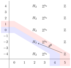
Figure 1: Second page for the Atiyah-Hirzebruch spectral sequence for the reduced K-homology of the horizon manifold on an isolated hypersurface singularity. We have denoted $H_{2}\coloneqq H_{2}(Y^{5})$, $b_{2}\coloneqq\operatorname{rk}(H_{2}\otimes\mathbb{Q})$, and shown the only differential that might potentially be non-vanishing. The entries shaded in blue are those contributing to $K_{0}(Y_{5})$, and those in pink are those contributing to $K_{1}(Y_{5})$.

The only potentially non-vanishing differential is indicated by $d^{3}$ in the drawing. This is the first non-vanishing differential, so it is a stable homology operation (see §4.L in Hatcher:478079 for a definition and proofs of some of the statements below) dual to a stable cohomology operation $d_{3}\colon H^{0}(Y_{5})\to H^{3}(Y_{5})$. Such operations are classified by $[K(\mathbb{Z},0),K(\mathbb{Z},3)]=[\mathbb{Z},K(\mathbb{Z},3)]=H^{3}(\mathbb{Z})=0$. So there is no non-vanishing stable homology operations acting on these degrees, and the spectral sequence stabilizes. There are no extension ambiguities either in going from the filtration to the K-theory group, so we conclude that $\tilde{K}_{0}(Y_{5})=H_{2}(Y_{5})=H^{3}(Y_{5})$.

The relation between the reduced and non-reduced K-homology groups is $K_{0}(Y_{5})=\mathbb{Z}\oplus\tilde{K}_{0}(Y_{5})$ (see for instance eq. (1.5) in Ruffino:2009zp ), so $K_{0}(Y_{5})=\mathbb{Z}\oplus\tilde{K}_{0}(Y_{5})$. Note also that $Y_{5}$ admits a Spin structure (since its normal bundle in the Calabi-Yau cone $X_{6}$ is trivial, and $X_{6}$ is Spin), and in particular a Spin^c structure, or in other words it is K-orientable. So we can apply Poincaré duality, and $K_{0}(Y_{5})=K^{1}(Y_{5})$. We conclude that

$$K^{1}(Y_{5})=H^{3}(Y_{5})\oplus H^{5}(Y_{5})$$ (58)

and similarly

$$K^{0}(Y_{5})=H^{0}(Y_{5})\oplus H^{2}(Y_{5})\,.$$ (59)

It is also clear that the K-theory groups of $\mathcal{M}_{4}$ agree with the formal sums of cohomology groups, since by the Chern isomorphism $K^{i}(\mathcal{M}_{4})\otimes\mathbb{Q}\cong\bigoplus_{n}H^{2n+i}(\mathcal{M}_{4};\mathbb{Q})$, and we are assuming that $\mathcal{M}_{4}$ has no torsion, so the relevant Atiyah-Hirzebruch spectral sequence has no non-vanishing differentials.

Finally, we can use the Künneth exact sequence in K-theory ATIYAH1962245

$$0\to\bigoplus_{i+j=m}K^{i}(X)\otimes K^{j}(Y)\to K^{m}(X\times Y)\to\bigoplus_{i+j=m+1}\operatorname{Tor}_{\mathbb{Z}}(K^{i}(X),K^{j}(Y))\to 0$$ (60)

to assemble these results together, and prove the statement in footnote 10 that we can use ordinary cohomology for classifying IIB flux in these backgrounds.

References

- (1) Y. Tachikawa, supersymmetric dynamics for pedestrians, 1312.2684.
- (2) D. Gaiotto, A. Kapustin, N. Seiberg and B. Willett, Generalized Global Symmetries, JHEP 02 (2015) 172, [1412.5148].
- (3) P. C. Argyres and M. R. Douglas, New phenomena in SU(3) supersymmetric gauge theory, Nucl. Phys. B 448 (1995) 93–126, [hep-th/9505062].
- (4) P. C. Argyres, M. Plesser, N. Seiberg and E. Witten, New N=2 superconformal field theories in four-dimensions, Nucl. Phys. B 461 (1996) 71–84, [hep-th/9511154].
- (5) T. Eguchi, K. Hori, K. Ito and S.-K. Yang, Study of N=2 superconformal field theories in four-dimensions, Nucl. Phys. B 471 (1996) 430–444, [hep-th/9603002].
- (6) T. Eguchi and K. Hori, N=2 superconformal field theories in four-dimensions and A-D-E classification, in Conference on the Mathematical Beauty of Physics (In Memory of C. Itzykson), pp. 67–82, 7, 1996. hep-th/9607125.
- (7) A. D. Shapere and C. Vafa, BPS structure of Argyres-Douglas superconformal theories, hep-th/9910182.
- (8) S. Cecotti, A. Neitzke and C. Vafa, R-Twisting and 4d/2d Correspondences, 1006.3435.
- (9) S. Cecotti and M. Del Zotto, On Arnold’s 14 ‘exceptional’ N=2 superconformal gauge theories, JHEP 10 (2011) 099, [1107.5747].
- (10) M. Del Zotto, More Arnold’s N = 2 superconformal gauge theories, JHEP 11 (2011) 115, [1110.3826].
- (11) S. Cecotti and M. Del Zotto, Infinitely many N=2 SCFT with ADE flavor symmetry, JHEP 01 (2013) 191, [1210.2886].
- (12) D. Xie, General Argyres-Douglas Theory, JHEP 01 (2013) 100, [1204.2270].
- (13) S. Cecotti, M. Del Zotto and S. Giacomelli, More on the N=2 superconformal systems of type , JHEP 04 (2013) 153, [1303.3149].
- (14) M. Del Zotto, C. Vafa and D. Xie, Geometric engineering, mirror symmetry and , JHEP 11 (2015) 123, [1504.08348].
- (15) D. Xie and S.-T. Yau, 4d N=2 SCFT and singularity theory Part I: Classification, 1510.01324.
- (16) S. Giacomelli, RG flows with supersymmetry enhancement and geometric engineering, JHEP 06 (2018) 156, [1710.06469].
- (17) B. Chen, D. Xie, S.-T. Yau, S. S. T. Yau and H. Zuo, 4D SCFT and singularity theory. Part II: complete intersection, Adv. Theor. Math. Phys. 21 (2017) 121–145, [1604.07843].
- (18) B. Chen, D. Xie, S. S. Yau, S.-T. Yau and H. Zuo, 4d SCFT and singularity theory Part III: Rigid singularity, Adv. Theor. Math. Phys. 22 (2018) 1885–1905, [1712.00464].
- (19) S. Gukov, C. Vafa and E. Witten, CFT’s from Calabi-Yau four folds, Nucl. Phys. B 584 (2000) 69–108, [hep-th/9906070].
- (20) C. Vafa and N. P. Warner, Catastrophes and the Classification of Conformal Theories, Phys. Lett. B 218 (1989) 51–58.
- (21) W. Lerche, C. Vafa and N. P. Warner, Chiral Rings in N=2 Superconformal Theories, Nucl. Phys. B 324 (1989) 427–474.
- (22) F. Albertini, M. Del Zotto, I. García Etxebarria and S. S. Hosseini, Higher Form Symmetries and M-theory, 2005.12831.
- (23) M. Del Zotto, I. García Etxebarria and S. S. Hosseini, “in preparation.”.
- (24) M. Caorsi and S. Cecotti, Special Arithmetic of Flavor, JHEP 08 (2018) 057, [1803.00531].
- (25) M. Caorsi and S. Cecotti, Homological classification of 4d = 2 QFT. Rank-1 revisited, JHEP 10 (2019) 013, [1906.03912].
- (26) S. Cecotti and M. Del Zotto, “On the classification of 4d N=2 QFTs. Parts I, II and III.”.
- (27) M. Caorsi and S. Cecotti, Homological -duality in 4d QFTs, Adv. Theor. Math. Phys. 22 (2018) 1593–1711, [1612.08065].
- (28) J. Milnor and P. Orlik, Isolated singularities defined by weighted homogeneous polynomials, Topology 9 (1970) 385 – 393.
- (29) C. P. Boyer, K. Galicki and S. R. Simanca, The sasaki cone and extremal sasakian metrics, 2007.
- (30) C. Boyer and K. Galicki, Sasakian Geometry. Oxford University Press, 2007. 10.1093/acprof:oso/9780198564959.001.0001.
- (31) I. García Etxebarria, B. Heidenreich and D. Regalado, IIB flux non-commutativity and the global structure of field theories, JHEP 10 (2019) 169, [1908.08027].
- (32) M. Del Zotto, J. J. Heckman, D. S. Park and T. Rudelius, On the Defect Group of a 6D SCFT, Lett. Math. Phys. 106 (2016) 765–786, [1503.04806].
- (33) D. R. Morrison, S. Schafer-Nameki and B. Willett, Higher-Form Symmetries in 5d, 2005.12296.
- (34) O. Aharony, N. Seiberg and Y. Tachikawa, Reading between the lines of four-dimensional gauge theories, JHEP 08 (2013) 115, [1305.0318].
- (35) S. Gukov, Trisecting non-Lagrangian theories, JHEP 11 (2017) 178, [1707.01515].
- (36) G. W. Moore and I. Nidaiev, The Partition Function Of Argyres-Douglas Theory On A Four-Manifold, 1711.09257.
- (37) C. Kozçaz, S. Shakirov and W. Yan, Argyres-Douglas Theories, Modularity of Minimal Models and Refined Chern-Simons, 1801.08316.
- (38) M. Buican and T. Nishinaka, On the superconformal index of Argyres–Douglas theories, J. Phys. A 49 (2016) 015401, [1505.05884].
- (39) C. Cordova and S.-H. Shao, Schur Indices, BPS Particles, and Argyres-Douglas Theories, JHEP 01 (2016) 040, [1506.00265].
- (40) C. Cordova, D. Gaiotto and S.-H. Shao, Infrared Computations of Defect Schur Indices, JHEP 11 (2016) 106, [1606.08429].
- (41) M. Buican and T. Nishinaka, Argyres-Douglas Theories, the Macdonald Index, and an RG Inequality, JHEP 02 (2016) 159, [1509.05402].
- (42) S. Cecotti, J. Song, C. Vafa and W. Yan, Superconformal Index, BPS Monodromy and Chiral Algebras, JHEP 11 (2017) 013, [1511.01516].
- (43) D. Xie, W. Yan and S.-T. Yau, Chiral algebra of Argyres-Douglas theory from M5 brane, 1604.02155.
- (44) D. Xie and W. Yan, Schur sector of Argyres-Douglas theory and -algebra, 1904.09094.
- (45) S. S. Razamat and M. Yamazaki, S-duality and the N=2 Lens Space Index, JHEP 10 (2013) 048, [1306.1543].
- (46) S. S. Razamat and B. Willett, Down the rabbit hole with theories of class , JHEP 10 (2014) 099, [1403.6107].
- (47) G. Festuccia, J. Qiu, J. Winding and M. Zabzine, supersymmetric gauge theory on connected sums of , JHEP 03 (2017) 026, [1611.04868].
- (48) G. Festuccia, J. Qiu, J. Winding and M. Zabzine, Twisting with a Flip (the Art of Pestunization), Commun. Math. Phys. 377 (2020) 341–385, [1812.06473].
- (49) S. Cecotti and C. Vafa, Classification of complete N=2 supersymmetric theories in 4 dimensions, Surveys in differential geometry 18 (2013) , [1103.5832].
- (50) M. Alim, S. Cecotti, C. Cordova, S. Espahbodi, A. Rastogi and C. Vafa, quantum field theories and their BPS quivers, Adv. Theor. Math. Phys. 18 (2014) 27–127, [1112.3984].
- (51) K. Maruyoshi and J. Song, deformations and RG flows of SCFTs, JHEP 02 (2017) 075, [1607.04281].
- (52) K. Maruyoshi and J. Song, Enhancement of Supersymmetry via Renormalization Group Flow and the Superconformal Index, Phys. Rev. Lett. 118 (2017) 151602, [1606.05632].
- (53) P. Agarwal, A. Sciarappa and J. Song, =1 Lagrangians for generalized Argyres-Douglas theories, JHEP 10 (2017) 211, [1707.04751].
- (54) S. Benvenuti and S. Giacomelli, Lagrangians for generalized Argyres-Douglas theories, JHEP 10 (2017) 106, [1707.05113].
- (55) F. Carta and A. Mininno, No go for a flow, JHEP 05 (2020) 108, [2002.07816].
- (56) C. Closset, S. Schaefer-Nameki and Y. Wang, “Coulomb and Higgs Branches from Canonical Singularities: Part 0.”.
- (57) D. S. Freed, G. W. Moore and G. Segal, Heisenberg Groups and Noncommutative Fluxes, Annals Phys. 322 (2007) 236–285, [hep-th/0605200].
- (58) D. S. Freed, G. W. Moore and G. Segal, The Uncertainty of Fluxes, Commun. Math. Phys. 271 (2007) 247–274, [hep-th/0605198].
- (59) G. W. Moore and E. Witten, Selfduality, Ramond-Ramond fields, and K theory, JHEP 05 (2000) 032, [hep-th/9912279].
- (60) J. Milnor, Singular Points of Complex Hypersurfaces. Princeton University Press, 1968.
- (61) A. Hatcher, Algebraic topology. Cambridge Univ. Press, Cambridge, 2000.
- (62) P. S. Aspinwall, D-branes on Calabi-Yau manifolds, in Progress in string theory. Proceedings, Summer School, TASI 2003, Boulder, USA, June 2-27, 2003, pp. 1–152, 3, 2004. hep-th/0403166. DOI.
- (63) M. Newman, Integral Matrices. Pure and applied mathematics : a series of monographs and textbooks. Academic Press, 1972.
- (64) C. M. Gordon and R. A. Litherland, On the signature of a link, Inventiones mathematicae 47 (1978) 53–69.
- (65) M. Caorsi and S. Cecotti, Categorical Webs and S-Duality in 4d QFT, Commun. Math. Phys. 368 (2019) 885–984, [1707.08981].
- (66) M. Barot, D. Kussin and H. Lenzing, The Grothendieck group of a cluster category, Journal of Pure and Applied Algebra 212 (2008) 33 – 46, [math/0606518].
- (67) B. Keller, The periodicity conjecture for pairs of Dynkin diagrams., Ann. Math. (2) 177 (2013) 111–170.
- (68) A. R. Iano-Fletcher, Working with weighted complete intersections, p. 101–174. London Mathematical Society Lecture Note Series. Cambridge University Press, 2000. 10.1017/CBO9780511758942.005.
- (69) M. Del Zotto and A. Hanany, Complete Graphs, Hilbert Series, and the Higgs branch of the 4d 2 SCFTs, Nucl. Phys. B 894 (2015) 439–455, [1403.6523].
- (70) S. Cecotti and C. Vafa, On classification of N=2 supersymmetric theories, Commun. Math. Phys. 158 (1993) 569–644, [hep-th/9211097].
- (71) Y. Wang and D. Xie, Classification of Argyres-Douglas theories from M5 branes, Phys. Rev. D 94 (2016) 065012, [1509.00847].
- (72) R. Switzer, Algebraic Topology: Homotopy and Homology. Classics in Mathematics. Springer, 2002.
- (73) F. F. Ruffino, Topics on the geometry of D-brane charges and Ramond-Ramond fields, JHEP 11 (2009) 012, [0909.0689].
- (74) M. Atiyah, Vector bundles and the Künneth formula, Topology 1 (1962) 245 – 248.