Electron-electron scattering and transport properties of spin-orbit coupled electron gas

Abstract

We calculate the electrical and thermal conductivity of a two-dimensional electron gas with strong spin–orbit coupling in which the scattering is dominated by electron–electron collisions. Despite the apparent absence of Galilean invariance in the system, the two-particle scattering does not affect the electrical conductivity above the band-crossing point where both helicity bands are filled. Below the band-crossing point where one helicity band is empty, switching on the electron–electron scattering leads only to a limited decrease of the electrical conductivity, so that its high-temperature value is independent of the scattering intensity. In contrast to this, thermal conductivity is not strongly affected by the spin-orbit coupling and exhibits only a kink as the Fermi level passes through the band-crossing point.

I Introduction

Two-dimensional (2D) systems with spin-orbit coupling (SOC) are key components of spintronics devices [1]. Apart from this, they possess a nontrivial structure of energy bands, which makes their charge- and heat-transport properties an interesting subject of research. So far, the main attention was focused on 2D SOC systems with purely elastic scattering [2, 3, 4, 5, 6]. In particular, it was found that the impurity-related resistivity exhibits an unconventional dependence on the electron density [2, 4]. Far less attention was given to the effects of inelastic scattering. Meanwhile it is of interest to find out how the electrical and heat conductivity are affected by electron–electron collisions. Typically, this scattering affects thermal conductivity but does not contribute to electrical conductivity in the absence of Umklapp processes, which change the total quasimomentum of colliding electrons by a reciprocal-lattice vector [7, 8] and take place only if the size of Fermi surface is comparable with that of the Brillouin zone. However due to the absence of Galilean invariance in systems with SOC, it may give a nonzero contribution to both of these quantities.

The Rashba spin-orbit coupling [9] splits the electron spectrum into the upper and lower helicity bands where the electron spin is locked to its momentum clockwise or counterclockwise. These bands cross at only one point in the momentum plane and the Fermi surface is doubly connected both above and below the corresponding energy. The effect of electron–electron scattering on the electric conductance in multiband electron systems was considered in a number of papers [10, 11, 12, 13] and it was found to give a contribution to the resistivity proportional to the square of temperature $T$. We show that this contribution exists in 2D SOC systems only below the band-crossing point. Moreover, it follows the $T^{2}$ dependence only if the electron–electron scattering is accompanied by a much stronger impurity scattering. As the temperature increases, the inelastic contribution saturates and the resistivity tends to a limiting value which is determined only by the elastic scattering, in violation of the Matthiessen’s rule. In contrast to this, the thermal conductivity limited by electron–electron scattering follows the $T^{-1}\ln^{-1}(E_{F}/T)$ temperature dependence characteristic of 2D systems [14] both below and above the band-crossing point, while its dependence on the chemical potential shows a kink at this point.

The rest of paper is organized as follows. In Section II we describe the model and write down the kinetic equations for the general case. In Section III we calculate the electrical conductivity in the presence of electron–electron and electron–impurity scattering and consider the limiting cases. In Section IV, the thermal conductivity is calculated in the presence of electron–electron scattering alone, and finally Section V contains the discussion of the results. The details of calculations are given in the Appendix.

II Model and general equations

We consider a 2D electron gas with strong Rashba spin-orbit coupling and weak electron–electron and electron–impurity interactions, which will be treated as perturbations. If the gas resides in the $xy$ plane, the unperturbed Hamiltonian is of the form

$$\hat{H}=\frac{\hat{p}_{x}^{2}+\hat{p}_{y}^{2}}{2m}+\alpha\,(\hat{\sigma}_{x}\hat{p}_{y}-\hat{\sigma}_{y}\hat{p}_{x}),$$ (1)

where $\alpha$ is the Rashba coupling constant and $\hat{\sigma}_{x,y}$ are the Pauli matrices. This Hamiltonian is easily diagonalized, and this results in two branches of spectrum

$$\varepsilon_{\nu}({\bm{p}})=\frac{p_{x}^{2}+p_{y}^{2}}{2m}+\nu\alpha\sqrt{p_{x}^{2}+p_{y}^{2}},\quad\nu=\pm 1,$$ (2)

which are shown in Fig. 1a. These branches give rise to two bands that intersect at only one point at the origin. While the upper branch $\varepsilon_{1}(p)$ monotonically increases, the lower branch exhibits a minimum $\varepsilon_{-1}(p_{0})=-E_{SO}$, where $p_{0}=m\alpha$ and $E_{SO}=m\alpha^{2}/2$. This suggests that the Fermi surface of the electron gas is doubly connected at the Fermi energy $E_{F}$ both below and above the band-crossing point and consists of two concentric circumferences. However at $E_{F}<0$, the occupied electron states form a ring between these contours and the directions of velocity at them are opposite. On the contrary, the velocities at both Fermi contours at $E_{F}>0$ are aligned in the same direction, see Fig. 1b. The corresponding wave functions are spinors whose components correspond to the spin projection on the $z$ axis $\sigma=\pm 1/2$

$$\psi_{{\bm{p}}\nu}({\bm{r}})=\frac{1}{\sqrt{2}}\,e^{i{\bm{p}}{\bm{r}}/\hbar}\binom{e^{i\chi_{{\bm{p}}}/2}}{\nu e^{-i\chi_{{\bm{p}}}/2}}$$ (3)

with $\chi_{{\bm{p}}}=\arctan(p_{x}/p_{y})$, so the spin is locked to the momentum and its component perpendicular to ${\bm{p}}$ is $\pm 1/2$. The sign of this component determines the helicity of the corresponding band.

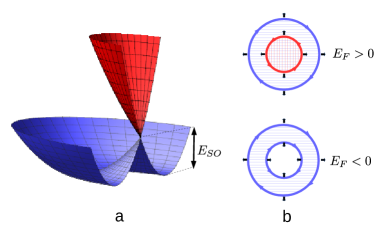
Figure 1: (a) 3D plot of the lower and upper helicity bands touching each other at the Dirac point. (b) The doubly connected Fermi surface above and below the Dirac point. The arrows show the directions of spin at the corresponding Fermi contours, the filled states are hatched with the colors of the corresponding band. Black arrows denote the directions of velocity.

A response of a fermionic system with weak scattering to slow-varying external fields is conveniently described by the standard kinetic equation of the form [15]

$$\frac{\partial f_{\nu}}{\partial t}+\frac{\partial\varepsilon_{\nu}}{\partial{\bm{p}}}\,\frac{\partial f_{\nu}}{\partial{\bm{r}}}+e{\bm{E}}\,\frac{\partial f_{\nu}}{\partial{\bm{p}}}=I_{\nu}^{imp}+I_{\nu}^{ee},$$ (4)

where $I_{\nu}^{imp}$ and $I_{\nu}^{ee}$ describe collisions of electrons with impurities and with each other. Note that the electron distribution function $f_{\nu}({\bm{p}},{\bm{r}})$ is the probability of finding an electron in the state $|\nu,{\bm{p}}\rangle$ at point ${\bm{r}}$ as in Ref. [5] and not the probability of finding there an electron with $z$ projection of spin $S_{z}=\pm 1/2$, as in many papers on spin transport [16]. This allows us to write the collision integrals in the standard form

$$I_{\nu}^{imp}({\bm{p}})=\sum_{\nu^{\prime}}\int\frac{d^{2}p^{\prime}}{(2\pi\hbar)^{2}}\,W_{{\bm{p}}{\bm{p}}^{\prime}}^{\nu\nu^{\prime}}\,\delta(\varepsilon_{\nu}-\varepsilon_{\nu^{\prime}})\\ \times\left[f_{\nu^{\prime}}({\bm{p}}^{\prime})-f_{\nu}({\bm{p}})\right]$$ (5)

and

$$I_{\nu}^{ee}({\bm{p}})=\sum_{\nu_{1}}\sum_{\nu_{2}}\sum_{\nu_{3}}\int\frac{d^{2}p_{1}}{(2\pi\hbar)^{2}}\int\frac{d^{2}p_{2}}{(2\pi\hbar)^{2}}\int d^{2}p_{3}\,\\ \times\delta({\bm{p}}+{\bm{p}}_{1}-{\bm{p}}_{2}-{\bm{p}}_{3})\,\delta(\varepsilon_{\nu}+\varepsilon_{\nu_{1}}-\varepsilon_{\nu_{2}}-\varepsilon_{\nu_{3}})\\ \times W^{\nu\nu_{1},\nu_{2}\nu_{3}}_{{\bm{p}}{\bm{p}}_{1},{\bm{p}}_{2}{\bm{p}}_{3}}\\ \times\bigl{[}(1-f)(1-f_{1})\,f_{2}\,f_{3}-f\,f_{1}\,(1-f_{2})(1-f_{3})\bigr{]}.$$ (6)

We assume that point-like impurities with concentration $n_{i}$ are described by the potential $U({\bm{r}})=U_{0}\,\delta({\bm{r}})$, so the electron–impurity scattering rate in the Born approximation calculated using $\psi_{\bm{\nu}}$ from Eq. (3) equals

$$W_{{\bm{p}}{\bm{p}}^{\prime}}^{\nu\nu^{\prime}}=\frac{\pi}{\hbar}\,n_{i}U_{0}^{2}\,[1+\nu\,\nu^{\prime}\cos(\widehat{{\bm{p}},{\bm{p}}^{\prime}})].$$ (7)

We also assume that due to the screening by a nearby gate, the interaction potential is short-ranged and may be written in the form $V({\bm{r}}-{\bm{r}}^{\prime})=V_{0}\,\delta({\bm{r}}-{\bm{r}}^{\prime})$. In the Born approximation, the scattering rate is proportional to the square of the difference between the matrix element of direct and exchange interaction $|\langle{\bm{p}}\nu,{\bm{p}}_{1}\nu_{1}|V|{\bm{p}}_{2}\nu_{2},{\bm{p}}_{3}\nu_{3}\rangle-\langle{\bm{p}}\nu,{\bm{p}}_{1}\nu_{1}|V|{\bm{p}}_{3}\nu_{3},{\bm{p}}_{2}\nu_{2}\rangle|^{2}$, where

$$\langle{\bm{p}}\nu,{\bm{p}}_{1}\nu_{1}|V|{\bm{p}}_{2}\nu_{2},{\bm{p}}_{3}\nu_{3}\rangle=\sum_{\sigma}\sum_{\sigma^{\prime}}\int d{\bm{r}}\int d{\bm{r}}^{\prime}\,\psi_{{\bm{p}}\nu}^{(\sigma)^{*}}({\bm{r}})\\ \times\psi_{{\bm{p}}_{1}\nu_{1}}^{(\sigma^{\prime})^{*}}({\bm{r}}^{\prime})\,V({\bm{r}}-{\bm{r}}^{\prime})\,\psi_{{\bm{p}}_{2}\nu_{2}}^{(\sigma)}({\bm{r}})\,\psi_{{\bm{p}}_{3}\nu_{3}}^{(\sigma^{\prime})}({\bm{r}}^{\prime}).$$ (8)

Making use of the explicit form of $\psi_{{\bm{p}}\nu}^{(\sigma)}({\bm{r}})$ Eq. (3), one easily obtains that

$$W^{\nu\nu_{1},\nu_{2}\nu_{3}}_{{\bm{p}}{\bm{p}}_{1},{\bm{p}}_{2}{\bm{p}}_{3}}=\frac{\pi}{2}\,\frac{V_{0}^{2}}{\hbar}\,[1-\nu\,\nu_{1}\cos(\widehat{{\bm{p}},{\bm{p}}_{1}})]\\ \times[1-\nu_{2}\,\nu_{3}\cos(\widehat{{\bm{p}}_{2},{\bm{p}}_{3}})].$$ (9)

As the spectrum of the system is rotationally symmetric, it is convenient to seek the linear response to the electric field $\bm{E}$ or the temperature gradient $\nabla T$ in the form

$$f_{\nu}({\bm{p}})=\bar{f}(\varepsilon_{\nu})+C_{\nu}(p)\,\bar{f}(\varepsilon_{\nu})\,[1-\bar{f}(\varepsilon_{\nu})]\cos\varphi,$$ (10)

where $\bar{f}$ is the equilibrium Fermi distribution, $p$ is the absolute value of ${\bm{p}}$, and $\varphi$ is the angle between $\bm{E}$ or $\nabla T$ and ${\bm{p}}$. The temperature is assumed to be low, so the nonequilibrium correction to $\bar{f}$ is nonzero only near the Fermi energy. With this substitution, the linearization of Eq. (6) results in the replacement of the distribution-dependent factor in it by the expression [17]

$$\left(C_{\nu_{2}}\cos\varphi_{2}+C_{\nu_{3}}\cos\varphi_{3}-C_{\nu}\cos\varphi-C_{\nu_{1}}\cos\varphi_{1}\right)\\ \times(1-\bar{f})(1-\bar{f}_{1})\,\bar{f}_{2}\,\bar{f}_{3}.$$ (11)

To proceed further, it is convenient to replace the integration variables ${\bm{p}}_{i}$ in Eq. (6) by $\varepsilon_{i}$ and $\varphi_{i}$. This replacement is straightforward at $\varepsilon>0$ because $p$ is a single-valued function of energy for both spectrum branches, but at $\varepsilon<0$ there is only one branch $\nu=-1$ and any value of $\varepsilon$ corresponds to two values of $p$ (see Fig. 1). To overcome this difficulty, we replace the branch indices $\nu$ in Eq. (4) by indices $\mu=\pm 1$ that correspond to the smaller and larger momentum for a given $\varepsilon$, hence $p_{\mu}(\varepsilon)$ are single-valued functions. A substitution of Eq. (10) into the collision integral with impurities Eq. (5) gives

$$I_{\mu}^{imp}(\varepsilon,\varphi)=-\Gamma_{0}\,\cos\varphi\,{\bar{f}}(1-\bar{f})\,\\ \times\frac{(p_{\mu}+2\,p_{-\mu})\,C_{\mu}+\operatorname{sgn}\varepsilon\,p_{-\mu}\,C_{-\mu}}{p_{\mu}+p_{-\mu}},$$ (12)

where $\Gamma_{0}=n_{i}U_{0}^{2}\,(p_{\mu}+p_{-\mu})/4\hbar^{3}|v_{\mu}|$ and $v_{\mu}^{-1}=\partial p_{\mu}/\partial\varepsilon$. Defined in this way, $\Gamma_{0}$ exhibits a peculiarity at the bottom of the lower helicity band due to the singularity in the density of states but is constant at high energies.

The calculation of the electron–electron collision integral is much more involved. Assuming that all the quantities except the distribution functions are energy-independent near the Fermi level and calculating the phase volume available for the scattering of electrons with given energies as in Ref. [18] (See Appendix A for the details), one finally obtains

$$I_{\mu}^{ee}(\varepsilon,\varphi)=2\cos\varphi\,\frac{\Gamma_{2}}{T^{2}}\int d\varepsilon^{\prime}\,K(\varepsilon,\varepsilon^{\prime})\\ \times\biggl{\{}Q_{\mu}\left[C_{\mu}(\varepsilon^{\prime})-C_{\mu}(\varepsilon)\right]+\Psi_{\mu}\,\frac{p_{\mu}\,C_{-\mu}(\varepsilon^{\prime})-p_{-\mu}\,C_{\mu}(\varepsilon^{\prime})}{p_{\mu}+p_{-\mu}}\\ +\sum_{\mu_{1}}R_{\mu\mu_{1}}\,\left[C_{\mu_{1}}(\varepsilon^{\prime})-C_{\mu_{1}}(-\varepsilon^{\prime})\right]\biggr{\}},$$ (13)

where $\Gamma_{2}(T)=V_{0}^{2}T^{2}\,(p_{\mu}+p_{-\mu})/32\pi^{3}\hbar^{5}|v_{\mu}|^{3}$ is the effective rate of electron–electron collisions,

$$K(\varepsilon,\varepsilon^{\prime})=\bigl{[}1-\bar{f}(\varepsilon)\bigr{]}\,\frac{\varepsilon-\varepsilon^{\prime}}{e^{(\varepsilon-\varepsilon^{\prime})/T}-1}\,\bar{f}(\varepsilon^{\prime}),$$ (14)

and all the energies are measured from $E_{F}$.

The first term in Eq. (13) is similar to the expression that arises in 2D conductors with a singly connected Fermi surface. The coefficient $Q_{\mu}$ diverges at $T\to 0$ and its most singular part is of the form

$$Q_{\mu}=4\,\frac{p_{\mu}+3\,p_{-\mu}}{p_{\mu}+p_{-\mu}}\,\ln\frac{E_{F}}{T},$$ (15)

but this term vanishes for $C_{\mu}(\varepsilon)={\rm const}$ and does not affect the electric resistivity if taken alone. The logarithmic singularity in the scattering rate of 2D electrons with singly connected Fermi surfaces is known to result from their head-on or small-angle collisions [19, 20]. In the case of doubly connected Fermi surface, the singularity in Eq. (15) arises not only from the scattering processes within the same Fermi contour, but also from the processes in which two pairs of the involved states, initial or final, belong to the same Fermi contours (see Fig. 2). In this figure, available for the scattering states are located at the intersections of two Fermi contours, one of which is shifted by the total momentum of colliding electrons. It is clearly seen that when their momenta are aligned or oppositely directed so that $\varphi-\varphi_{1}=0$ or $\varphi-\varphi_{1}=\pi$, these contours become tangent rather than intersecting, hence the phase space available for scattering sharply increases. Depending on the specific indices $\nu\ldots\nu_{3}$, one of these singularities is suppressed by the angle-dependent factors in Eq. (9).

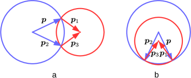
Figure 2: The origin of the logarithmic singularity in Eq. (15). If an electron with momentum ${\bm{p}}$ from the outer Fermi contour collides with an electron with momentum ${\bm{p}}_{1}$ from the inner contour and they are scattered again to different contours, the states ${\bm{p}}_{1}$ must lie at the intersections of two Fermi contours, one of which is shifted by ${\bm{p}}+{\bm{p}}_{1}$. If ${\bm{p}}$ and ${\bm{p}}_{1}$ are parallel or antiparallel, these contours become externally or internally tangent rather than intersecting, and hence the number of states participating in the scattering sharply increases.

The third term in Eq. (13) also presents an extension of a similar contribution for a singly connected Fermi surface and contains low-temperature logarithmic singularities of the form

$$R_{\mu\mu_{1}}=8\bigl{[}\operatorname{sgn}E_{F}-2\,\delta_{\mu\mu_{1}}\Theta(E_{F})\bigr{]}\,\frac{p_{\mu_{1}}}{p_{\mu}+p_{\mu_{1}}}\,\ln\frac{E_{F}}{T},$$ (16)

but is zero for any even $C_{\mu}(\varepsilon)$. This term does not contribute to the electric conductivity but is essential when dealing with thermal transport.

The second term in Eq. (13) has no analog for a singly connected Fermi surface and is of special interest because it does not vanish for arbitrary energy-independent $C_{\mu}$. The specific form of this term is best understood by comparing the first factor in Eq. (11) with the argument of the momentum delta function in Eq. (6). As this argument must be zero for all collisions that satisfy momentum conservation, its projection on the direction of $\bm{E}$ or $\nabla T$ immediately gives

$$p_{\mu_{2}}\cos\varphi_{2}+p_{\mu_{3}}\cos\varphi_{3}-p_{\mu}\cos\varphi-p_{\mu_{1}}\cos\varphi_{1}=0.$$

Therefore the first factor in Eq. (11) turns into zero if $C_{\mu}/p_{\mu}=C_{\mu_{1}}/p_{\mu_{1}}=C_{\mu_{2}}/p_{\mu_{2}}=C_{\mu_{3}}/p_{\mu_{3}}$ and hence the resulting expression is proportional to $p_{\mu}\,C_{-\mu}(\varepsilon^{\prime})-p_{-\mu}\,C_{\mu}(\varepsilon^{\prime})$. The factors $\Psi_{\mu}$ are given by integrals that can be calculated only numerically (see Appendix A). The $\Psi_{\mu}(E_{F})$ curves are shown in Fig. 3. Both of them exhibit a logarithmic singularity at the bottom of the lower helicity band $E_{F}=-S_{SO}$ and tend to the same value $\Psi_{\pm 1}=16$ at $E_{F}\gg E_{SO}$. However $\Psi_{1}$ monotonically decreases with increasing $E_{F}$, while $\Psi_{-1}$ first decreases to zero at $E_{F}=0$ and then increases again. The kinks in $\Psi_{\mu}$ at $E_{F}<0$ is due to the closure of scattering channels with three electron states at the inner Fermi contour and one at the outer contour at $p_{1}=3\,p_{-1}$. Note that unlike $Q_{\mu}$ and $R_{\mu\mu_{1}}$, $\Psi_{\mu}$ do not have a low-temperature logarithmic singularity. This is because at $\varphi-\varphi_{1}=0$ and $\varphi-\varphi_{1}=\pi$, the quadrangles in Fig. 2 collapse into segments and the first factor in Eq. (11) turns into zero regardless of the ratio of $C_{1}$ to $C_{-1}$. This term appears to be of crucial importance in calculating the electrical conductivity of 2D electron gas.

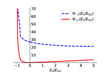
Figure 3: The dependences of $\Psi_{\mu}$ on $E_{F}/E_{SO}$.

III Electrical conductivity

In the linear approximation in the electric field, the Boltzmann equation Eq. (4) assumes the form

$$eEv_{\mu}\,\cos\varphi\,\frac{\partial\bar{f}}{\partial\varepsilon}=I_{\mu}^{imp}(\varepsilon,\varphi)+I_{\mu}^{ee}(\varepsilon,\varphi),$$ (17)

where $I_{\mu}^{imp}$ and $I_{\mu}^{ee}$ are given by Eqs. (12) and (13). As the perturbation in left-hand side is an even function of $\varepsilon$ and both collision integrals conserve parity, the solutions for $C_{\mu}$ are also even in $\varepsilon$ and the last term in Eq. (13) may be discarded. To solve the system of resulting integral equations, we use the method pioneered in [21] and introduce new variables

$$\rho_{\mu}(\varepsilon)=[\bar{f}\,(1-\bar{f})]^{1/2}\,C_{\mu}(\varepsilon).$$ (18)

As a result, the kernel $K(\varepsilon,\varepsilon^{\prime})$ of the integral in Eq. (13) is replaced by a function of $\varepsilon^{\prime}-\varepsilon$, and the integral equations (17) may be brought to the differential form by the Fourier transform

$$\tilde{\rho}_{\mu}(u)=\int d\varepsilon\,e^{-i\varepsilon u}\,\rho_{\mu}(\varepsilon).$$ (19)

Furthermore, an introduction of the new independent variable $\xi=\tanh(\pi Tu)$ brings these equations to the form

$$\Gamma_{2}\left[Q_{\mu}\left(\hat{L}+2\right)\,\tilde{\rho}_{\mu}-2\,\Psi_{\mu}\,\frac{p_{-\mu}\,\tilde{\rho}_{\mu}-p_{\mu}\,\tilde{\rho}_{-\mu}}{p_{\mu}+p_{-\mu}}\right]\\ -\frac{1}{\pi^{2}}\,\frac{\Gamma_{0}}{1-\xi^{2}}\,\frac{(p_{\mu}+2p_{-\mu})\,\tilde{\rho}_{\mu}+\operatorname{sgn}E_{F}\,p_{-\mu}\,\tilde{\rho}_{-\mu}}{p_{\mu}+p_{-\mu}}\\ =-\pi^{-1}{eEv_{\mu}}\,(1-\xi^{2})^{-1/2},$$ (20)

where $\hat{L}$ stands for the differential operator

$$\hat{L}\,\phi=\frac{\partial}{\partial\xi}\biggl{[}(1-\xi^{2})\,\frac{\partial\phi}{\partial\xi}\biggr{]}-\frac{\phi}{1-\xi^{2}}.$$ (21)

The eigenfunctions of this operator involve Jacobi polynomials and are proportional [22] to $(1-\xi^{2})^{1/2}\,P_{m}^{(1,1)}(\xi)$ with the corresponding eigenvalues $-(m+1)(m+2)$. As $\tilde{\rho}_{\mu}$ are even functions of $\xi$, it is convenient to present them as series expansions over the normalized even-number eigenfunctions $\phi_{m}$ of operator $\hat{L}$

$$\tilde{\rho}_{\mu}(\xi)=\sum_{m=0}^{\infty}\gamma_{\mu m}\,\phi_{2m}(\xi).$$ (22)

A substitution of these expansions into Eqs. (20) and their projection on the same set of functions results in an infinite system of equations

$$2\,\Gamma_{2}\biggl{[}m\,(2m+3)\,Q_{\mu}\,\gamma_{\mu m}+\Psi_{\mu}\,\frac{p_{-\mu}\,\gamma_{\mu m}-p_{\mu}\,\gamma_{-\mu m}}{p_{\mu}+p_{-\mu}}\Biggr{]}\\ +\frac{\Gamma_{0}}{\pi^{2}}\sum_{n=0}^{\infty}Y_{mn}\,\frac{(p_{\mu}+2p_{-\mu})\,\gamma_{\mu n}+\operatorname{sgn}E_{F}\,p_{-\mu}\,\gamma_{-\mu n}}{p_{\mu}+p_{-\mu}}\\ =\pi^{-1}\,{eEv_{\mu}}\,X_{m},$$ (23)

where $X_{m}$ and $Y_{mn}$ depend only on $m$ and $n$ with explicit expressions given in Appendix B. Once the quantities $\gamma_{\mu m}$ are known, the distribution functions $f_{\mu}$ may be restored using Eqs. (22), (19), (18), and (10), which results in the density of electric current of the form

$$j=\frac{e}{8\pi^{2}\hbar^{2}}\sum_{\mu}p_{\mu}\operatorname{sgn}v_{\mu}\sum_{m}X_{m}\,\gamma_{\mu m}.$$ (24)

First consider the case where only the impurity scattering is present. The solution of Eq. (23) is

$$\tilde{\rho}_{\mu}^{imp}(\xi)=\frac{2\sqrt{3}\pi}{3}\,\frac{eEv_{\mu}}{\Gamma_{0}}\,\frac{p_{\mu}}{p_{\mu}+p_{-\mu}}\,\phi_{0}(\xi),$$ (25)

which results in the current density

$$j^{imp}=\frac{1}{4\pi}\,E\,\frac{e^{2}}{\hbar^{2}}\,\frac{v_{1}}{\Gamma_{0}}\,\frac{p_{1}^{2}+p_{-1}^{2}}{p_{1}+p_{-1}}$$ (26)

equivalent to the one obtained in Refs. [2, 4].

As $v_{\mu}$ are equal and positive for both Fermi contours at $E_{F}>0$, the solution Eq. (25) also turns into zero the term resulting from electron–electron collisions, so they do not affect the resistivity. This is due to the specific form of the electron distribution Eq. (25), which results from the particular probability of impurity scattering Eq. (7) and hence from the assumption of short-ranged impurity potential. Therefore this is not a universal property of 2D SOC electron systems (see Appendix C).

Below the band-crossing point, $v_{\mu}$ are equal in magnitude but are of opposite signs at both Fermi contours, hence the distribution Eq. (25) does not turn $I^{ee}_{\mu}$ into zero and the electron–electron scattering is essential. First we calculate the correction to the current from electron–electron collisions treating them as a perturbation in the case of a strong impurity scattering. This is conveniently done by means of Eq. (20) as the zero-approximation distribution (25) eliminates in it the term proportional to $Q_{\mu}$ that contains a differential operator. Therefore the solution for the first-order correction is straightforward, and one obtains the corrections to $\tilde{\rho}_{\mu}^{imp}(\xi)$ proportional to $(1-\xi^{2})^{3/2}$. The correction to the current

$$\delta j^{ee}=-\frac{2\pi e^{2}E}{3\,\hbar^{2}}\,\frac{\Gamma_{2}}{\Gamma_{0}^{2}}\,v_{1}\,\frac{p_{1}\,p_{-1}\left[p_{-1}^{2}\,\Psi_{-1}+p_{1}^{2}\,\Psi_{1}\right]}{(p_{1}+p_{-1})^{3}}.$$ (27)

is proportional to $T^{2}$ in agreement with [13] and does not contain a logarithm of $T$ as one might expect for a 2D system. Quite predictably, it tends to zero at the band-crossing point where the inner Fermi contour shrinks to a point and $p_{-1}=0$. It diverges as the Fermi level approaches the bottom of the lower helicity band due to the singularity in the density of states, but it only means that the perturbative approach fails there.

Consider now the opposite case of strong electron–electron scattering. It is easily seen that if one simply sets $\Gamma_{0}=0$, the system of equations (23) for $m=0$ becomes degenerate because its left-hand side is made zero by any distribution with $\gamma_{10}/\gamma_{-10}=p_{1}/p_{-1}$. To avoid this, one has to introduce in Eqs. (23) a very weak impurity scattering. It results only in corrections of the order $1/\Gamma_{2}$ for $\gamma_{\mu m}$ with $m\neq 0$, but the leading terms in $\gamma_{\mu 0}$ appear to be proportional to $1/\Gamma_{0}$. The leading contribution to the current density equals

$$j^{ee}=E\,\frac{e^{2}}{4\pi\hbar}\,\frac{v_{1}\,(p_{1}+p_{-1})}{\hbar\Gamma_{0}}\\ \times\frac{(p_{1}^{2}-p_{-1}^{2})(\Psi_{-1}-\Psi_{1})}{(p_{1}^{2}-p_{-1}^{2})(\Psi_{-1}-\Psi_{1})+2\,p_{1}\,p_{-1}\,(\Psi_{1}+\Psi_{-1})}.$$ (28)

Though this current density is inversely proportional to the impurity-scattering rate like Eq. (26), it is somewhat smaller and has a different dependence on $E_{F}$ (see Fig. 4). The ratio $j^{imp}/j^{ee}$ reaches its minimum value $\sim 0.66$ at $E_{F}/E_{SO}\approx-0.85$. The two curves merge at $E_{F}=-E_{SO}$ and $E_{F}=0$. The temperature dependence of conductivity may be obtained by truncating the infinite series Eq. (22) to a finite number of terms and numerically solving the system (23). The resulting curve is shown in Fig. 5 for $E_{F}=-0.85E_{SO}$ and exhibits a saturation of conductivity with increasing temperature.

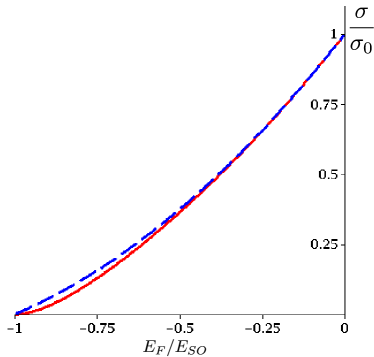
Figure 4: The dependences of conductivity $\sigma$ on $E_{F}$ in the case of strong (solid line) and weak (dashed line) electron–electron scattering for the same impurity-scattering rate given by Eqs. (28) and (26). The conductivity is normalized to its value $\sigma_{0}=e^{2}\hbar\,\alpha^{2}/\pi n_{i}\,U_{0}^{2}$ at $E_{F}=0$. At $E_{F}>0$, the electron–electron scattering has no effect on $\sigma$.

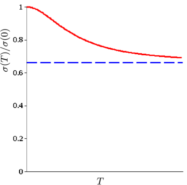
Figure 5: The temperature dependence of normalized conductivity for $E_{F}=-0.85\,E_{SO}$ obtained by a numerical solution of Eqs. (23).

IV Thermal conductivity

As electron–electron collisions do not conserve heat flux, they generally limit thermal conductivity even in the absence of additional scattering mechanisms, so there is no need to include an additional impurity scattering. If the perturbation is caused by a gradient of temperature, the equation for the linear response is of the form

$$v_{\mu}\,|\nabla T|\,\frac{\varepsilon}{T^{2}}\,\bar{f}\,(1-\bar{f})\,\cos\varphi=I_{\mu}^{ee}$$ (29)

We seek again the distribution function of electrons in the form (10), but now $C_{\mu}$ are odd functions of $\varepsilon$ according to the symmetry of perturbation. For this reason, the last term in Eq. (13) does not vanish, but instead the second term may be omitted because it does not contain the $\ln(E_{F}/T)$ factor. Hence

$$I^{ee}_{\mu}=-8\,\cos\varphi\,\frac{\Gamma_{2}}{T^{2}}\,\ln\frac{E_{F}}{T}\int d\varepsilon^{\prime}\,K(\varepsilon,\varepsilon^{\prime})\\ \times\Bigl{[}(p_{\mu}+3\,p_{-\mu})\,C_{\mu}(\varepsilon)+(p_{\mu}-p_{-\mu})\,C_{\mu}(\varepsilon^{\prime})\\ -4\,\operatorname{sgn}E_{F}\,p_{-\mu}\,C_{-\mu}(\varepsilon^{\prime})\Bigr{]}(p_{\mu}+p_{-\mu})^{-1}.$$ (30)

By repeating the steps described by Eqs. (18) and (19) in the previous section, one arrives at the equation

$$\left[(p_{\mu}+3\,p_{-\mu})\,\hat{L}-2\,(p_{\mu}-p_{-\mu})+8\,\operatorname{sgn}E_{F}\,p_{-\mu}\right]\tilde{\rho}_{\mu}\\ =-\frac{i}{4}\,\frac{|\nabla T|\,v_{\mu}\,(p_{\mu}+p_{-\mu})}{\Gamma_{2}\,\ln(E_{F}/T)}\,\frac{\xi}{\sqrt{1-\xi^{2}}}.$$ (31)

As the right-hand side of this equation is an odd function of $\xi$, this equation can be solved by expanding $\tilde{\rho}_{\mu}$ over odd-number eigenfunctions $\phi_{2m+1}$ of operator $\hat{L}$. In the absence of impurity scattering, this system becomes uncoupled for different $m$ and is easily solved. The heat flux $\bf q$ is obtained as an infinite series over $m$, and the thermal conductivity $\kappa=q/|\nabla T|$ is of the form

$$\kappa=-\frac{T\,v_{1}\,(p_{1}+p_{-1})}{64\pi\hbar^{2}\Gamma_{2}\ln(E_{F}/T)}\sum_{m=0}^{\infty}\frac{4m+5}{S_{m}\,(S_{m}+1)}\\ \times\frac{(3S_{m}-1)(p_{1}+p_{-1})^{2}-4\,(S_{m}-3)\,p_{1}\,p_{-1}}{(3S_{m}-1)(p_{1}+p_{-1})^{2}+4\,(S_{m}-3)\,p_{1}\,p_{-1}},$$ (32)

where $S_{m}=(m+1)(2m+3)$. The temperature dependence of thermal conductivity follows the same $[T\ln(E_{F}/T)]^{-1}$ law as for 2D electron gas without SOC [14]. Its dependence on the Fermi level is shown in Fig. 6. Though the expression for $\kappa$ (32) does not explicitly depend on the sign of $E_{F}$, it exhibits a kink at $E_{F}=0$ because the derivative of the smaller Fermi momentum $dp_{-1}/dE_{F}$ changes its sign at this point.The relative change of the slope is

$$\frac{d\kappa/dE_{F}|_{+0}}{d\kappa/dE_{F}|_{-0}}\approx 0.83$$ (33)

This relation is free from any unknown parameters and can serve as an experimental test of the considered model. The negative jump of the derivative $d\kappa/dE_{F}$ results from the peculiarity in the scattering of electrons on the outer Fermi contour by the electrons on the inner Fermi contour at the band-crossing point. On the contrary, the heat flux carried by the electrons on the inner contour turns into zero at this point and therefore exhibits a positive jump of derivative.

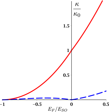
Figure 6: The dependence of the thermal conductivity $\kappa$ on the Fermi energy given by Eq. (32). The dashed line shows the contribution from the inner Fermi contour. The thermal conductivity is normalized to its value $\kappa_{0}\approx 2.77\,\hbar^{3}\alpha^{4}/V_{0}^{2}T$ at $E_{F}=0$.

V Discussion

The effects considered in previous sections are best observed in 2D electron systems with strong SOC like InAS, which exhibits Rashba parameter $\hbar\alpha=1.2\,{\rm eV\AA}$ [23]. The temperature should be sufficiently low to suppress the electron–phonon scattering, which is proportional to $T^{4.5}$ in 2D systems [24]. Furthermore, the parameter of electron–electron scattering $\Gamma_{2}$ has to be larger than the impurity-scattering parameter $\Gamma_{0}$. At $T=2$ K, the electron concentration $10^{10}$ cm^-2, and the gas–gate distance of 20 nm, one obtains the transport scattering length $l_{ee}=|v_{\mu}|/\Gamma_{2}\sim 250$ nm. This is well below the elastic mean free path of 800 nm reported very recently in InAs 2D electron gas in Ref. [25], so the regime of dominant electron–electron scattering may be achieved for realistic parameters of the system.

While the thermal transport in 2D electron systems with strong electron–electron scattering is only slightly affected by SOC, its effects on charge transport in these systems are much less trivial. In the absence of SOC, this type of scattering does not affect charge transport at all because of momentum conservation. One may think that the emergence of a double Fermi contour will lift this constraint and the electron–electron collisions will become the dominant mechanism of current relaxation, but this is not the case. The reason is that a certain type of perturbation involving the electron distributions on both contours is not affected by them. As a result, increasing the intensity of electron–electron scattering does not fully suppress the current induced by applied electric field [*[Forsingle-bandmetals, itwasnotedin][]Maslov11]. Instead, this current decreases only to a finite value, which is determined by other mechanisms of scattering and depends on their details as well as those of electron–electron interaction. Though we made explicit calculations for a point-like interaction potential, these conclusions are qualitatively valid for its arbitrary shape.

The partial nature of current relaxation via electron–electron collisions is not unique to 2D systems with SOC. The existence of the perturbation immune to electron–electron collisions is a general property of systems with multiply connected Fermi surface, which results from the momentum and energy conservation and the structure of the electron–electron collision integral. This perturbation is unaffected even by triple electronic collisions [27] because they obey the same conservation laws. Therefore a similar partial relaxation of the current by these collisions may be observed in a broad class of 2D and 3D systems. Possible candidates are graphene with Zeeman-shifted Dirac points or 2D systems without SOC but with two filled transverse subbands.

Appendix A Angular integration in the collision integral

Here we present a derivation of the collision integral Eq. (13) for the case where $E_{F}>0$. The extension to negative $E_{F}$ is straightforward. We start with Eqs. (6) and (11) and step by step eliminate the integrations over momentum angles in them. When integrating over ${\bm{p}}_{2}$ and ${\bm{p}}_{3}$, it is convenient to measure them with respect to the sum ${\bm{p}}_{\Sigma}\equiv{\bm{p}}+{\bm{p}}_{1}$. It is easily seen from the cosine theorem that

$$\cos(\varphi_{2}-\varphi_{3})=\frac{p_{\Sigma}^{2}-p_{2}^{2}-p_{3}^{2}}{2\,p_{2}\,p_{3}},$$ (34)

where

$$p_{\Sigma}^{2}=p^{2}+p_{1}^{2}+2\,p\,p_{1}\cos(\varphi_{1}-\varphi).$$ (35)

For brevity, we use here the notation $p_{i}\equiv p_{\mu_{i}}(\varepsilon_{i})$. The cosines of $\varphi_{2}$ and $\varphi_{3}$ are conveniently presented in the form

$$\cos\varphi_{2,3}=\cos(\varphi_{2,3}-\varphi_{\Sigma})\,\cos\varphi_{\Sigma}\\ -\sin(\varphi_{2,3}-\varphi_{\Sigma})\,\sin\varphi_{\Sigma}.$$ (36)

It should be noted that the terms with $\sin(\varphi_{2,3}-\varphi_{\Sigma})$ vanish upon the integration over ${\bm{p}}_{2,3}$ because of the symmetry, and the corresponding cosine may be expressed through the cosine theorem as

$$\cos(\varphi_{2,3}-\varphi_{\Sigma})=\frac{p_{{2,3}}^{2}+p_{\Sigma}^{2}-p_{{3,2}}^{2}}{2\,p_{{2,3}}\,p_{\Sigma}},$$ (37)

while

$$\cos\varphi_{\Sigma}=\frac{p\cos\varphi+p_{1}\cos\varphi_{1}}{p_{\Sigma}}.$$ (38)

Therefore the two last cosine-dependent factors may be put before the integrals over ${\bm{p}}_{2}$ and ${\bm{p}}_{3}$ . The remaining integral has been calculated in Ref. [18] and equals

$$\int\frac{d^{2}p_{2}}{(2\pi\hbar)^{2}}\int\frac{d^{2}p_{3}}{(2\pi\hbar)^{2}}\,\delta(\varepsilon_{\mu_{2}{\bm{p}}_{2}}-\varepsilon_{2})\,\delta(\varepsilon_{\mu_{3}{\bm{p}}_{3}}-\varepsilon_{3})\\ \times\delta({\bm{p}}+{\bm{p}}_{1}-{\bm{p}}_{2}-{\bm{p}}_{3})=\frac{1}{4\pi^{4}\hbar^{4}}\,\frac{p_{2}\,p_{3}}{|v_{2}\,v_{3}|}\,\frac{\Theta(\Delta)}{\sqrt{\Delta}},$$ (39)

where

$$\Delta=\left[p_{\Sigma}^{2}-(p_{2}-p_{3})^{2}\right]\left[(p_{2}+p_{3})^{2}-p_{\Sigma}^{2}\right].$$ (40)

Hence the integral Eq. (6) may be brought to the form

$$I_{\mu}^{ee}(\varepsilon,\varphi)=\cos\varphi\,\frac{V_{0}^{2}}{16\pi^{3}\hbar^{5}}\sum_{\mu_{1}}\sum_{\mu_{2}}\sum_{\mu_{3}}\int d\varepsilon_{1}\int d\varepsilon_{2}\\ \times\int d\varepsilon_{3}\,\delta(\varepsilon+\varepsilon_{1}-\varepsilon_{2}-\varepsilon_{3})\,(1-\bar{f})(1-\bar{f}_{1})\,\bar{f}_{2}\,\bar{f}_{3}\\ \times p_{1}\,\int_{-\pi}^{\pi}d\chi\,(1-\mu\,\mu_{1}\cos\chi)\left|{\rm Re}\,\frac{{\cal D}_{\mu..\mu_{3}}^{\mu_{2}\mu_{3}/2}(\chi)}{v_{1}\,v_{2}\,v_{3}}\right|\\ \times\Bigl{[}\lambda_{\mu..\mu_{3}}\,C_{\mu_{2}}+\bar{\lambda}_{\mu..\mu_{3}}\,C_{\mu_{3}}-\cos\chi\,C_{\mu_{1}}-C_{\mu}\Bigr{]},$$ (41)

where $\mu..\mu_{3}$ stands for $\mu\mu_{1}\mu_{2}\mu_{3}$,

$${\cal D}_{\mu..\mu_{3}}=\frac{(p_{2}+p_{3})^{2}-p^{2}-p_{1}^{2}-2\,p\,p_{1}\cos\chi}{p^{2}+p_{1}^{2}+2\,p\,p_{1}\cos\chi-(p_{2}-p_{3})^{2}},$$ (42)

$$\lambda_{\mu..\mu_{3}}=\frac{1}{2}\,\frac{p_{2}^{2}-p_{3}^{2}+p^{2}+p_{1}^{2}+2\,p\,p_{1}\cos\chi}{p^{2}+p_{1}^{2}+2\,p\,p_{1}\cos\chi}\\ \times(p+p_{1}\cos\chi)/{p_{2}},$$ (43)

and

$$\bar{\lambda}_{\mu\mu_{1}\mu_{2}\mu_{3}}\equiv\lambda_{\mu\mu_{1}\mu_{3}\mu_{2}}.$$ (44)

If $I_{\mu}^{ee}$ is calculated in the leading approximation to the order $T^{2}$, all the quantities except the distribution functions may be considered as energy-independent near the Fermi level. Therefore the integration over $\varepsilon_{1}$ , $\varepsilon_{2}$ , and $\varepsilon_{3}$ is easily performed and the collision integral (6) is brought to the form

$$I_{\mu}^{ee}(\varepsilon,\varphi)=\cos\varphi\,\frac{V_{0}^{2}}{16\pi^{3}\hbar^{5}}\sum_{\mu_{1}}\sum_{\mu_{2}}\sum_{\mu_{3}}\\ \times p_{1}\,\int_{-\pi}^{\pi}d\chi\,(1-\mu\,\mu_{1}\cos\chi)\left|{\rm Re}\,\frac{{\cal D}_{\mu..\mu_{3}}^{\mu_{2}\mu_{3}/2}(\chi)}{v_{1}\,v_{2}\,v_{3}}\right|\\ \times\int d\varepsilon^{\prime}\,\Bigl{\{}K(\varepsilon,\varepsilon^{\prime})\bigl{[}\lambda_{\mu..\mu_{3}}\,C_{\mu_{2}}(\varepsilon^{\prime})+\bar{\lambda}_{\mu..\mu_{3}}\,C_{\mu_{3}}(\varepsilon^{\prime})\\ -C_{\mu}(\varepsilon)\bigr{]}-K(\varepsilon,-\varepsilon^{\prime})\cos\chi\,C_{\mu_{1}}(\varepsilon^{\prime})\Bigr{\}},$$ (45)

where $K(\varepsilon,\varepsilon^{\prime})$ is given by Eq. (14). Upon regrouping the terms in Eq. (45), one obtains Eq. (13), where

$$Q{\mu}=\sum_{\mu_{1}}\sum_{\mu_{2}}\sum_{\mu_{3}}\frac{p_{\mu_{1}}}{p_{\mu}+p_{-\mu}}\int_{-\pi}^{\pi}d\chi\,(1-\mu\,\mu_{1}\cos\chi)\\ \times\Theta({\cal D}_{\mu..\mu_{3}})\,{\cal D}_{\mu..\mu_{3}}^{\mu_{2}\mu_{3}/2},$$ (46)

$$\Psi_{\mu}=\sum_{\mu_{1}}\sum_{\mu_{2}}\sum_{\mu_{3}}\frac{p_{\mu_{1}}}{p_{-\mu}}\int_{-\pi}^{\pi}d\chi\,(1-\mu\,\mu_{1}\cos\chi)\,\Theta({\cal D}_{\mu..\mu_{3}})\\ \times{\cal D}_{\mu..\mu_{3}}^{\mu_{2}\mu_{3}/2}\,\left(1-\delta_{\mu\mu_{1}}\cos\chi-2\,\delta_{\mu\mu_{2}}\lambda_{\mu..\mu_{3}}\right),$$ (47)

and

$$R_{\mu\mu_{1}}=\sum_{\mu_{2}}\sum_{\mu_{3}}\frac{p_{\mu_{1}}}{p_{\mu}+p_{-\mu}}\int_{-\pi}^{\pi}d\chi\,(1-\mu\,\mu_{1}\cos\chi)\\ \times\Theta({\cal D}_{\mu..\mu_{3}})\,{\cal D}_{\mu..\mu_{3}}^{\mu_{2}\mu_{3}/2}\,\cos\chi.$$ (48)

For negative $E_{F}$ , these quantities are given by similar expressions except that the prefactors $\mu\mu_{1}$ to $\cos\chi$ and the products $\mu_{2}\mu_{3}$ in the exponents in Eqs. (46) - (48) are replaced by 1.

Appendix B Expressions for eigenfunctions and expansion coefficients

The normalized eigenfunctions of differential operator $\hat{L}$ defined in Eq. (21) are given by equation

$$\phi_{m}(\xi)=\sqrt{\frac{(2m+3)(m+2)}{8\,(m+1)}}\sqrt{1-\xi^{2}}\,P_{m}^{(1,1)}(\xi),$$ (49)

where $P_{m}^{(1,1)}(\xi)$ are Jacobi polynomials. The quantity $(1-\xi^{2})^{-1/2}$ in the right-hand side of Eq. (20) may be presented as a series

$$\frac{1}{\sqrt{1-\xi^{2}}}=\sum_{m=0}^{\infty}X_{m}\,\phi_{2m}(\xi),$$ (50)

where

$$X_{m}=\int_{-1}^{1}d\xi\,\frac{\phi_{2m}(\xi)}{\sqrt{1-\xi^{2}}}=\sqrt{\frac{4m+3}{(2m+1)(m+1)}}.$$ (51)

The matrix elements of $1/(1-\xi^{2})$ between the eigenfunctions of $\hat{L}$ are given by the equation

$$Y_{mn}=\int_{-1}^{1}d\xi\,\frac{\phi_{2m}(\xi)\,\phi_{2n}(\xi)}{1-\xi^{2}}=\frac{\min(m,n)+1/2}{\max(m,n)+1}\\ \times\sqrt{\frac{(4m+3)(m+1)(4n+3)(n+1)}{(2m+1)(2n+1)}}.$$ (52)

Appendix C Momentum-dependent impurity scattering

If the impurities are rotationally symmetric but of finite size, the matrix element of electron–impurity interaction depends on the change of electron momentum ${\bm{p}}-{\bm{p}}^{\prime}$ and hence Eq. (7) assumes the form

$$W_{{\bm{p}}{\bm{p}}^{\prime}}^{\nu\nu^{\prime}}=\frac{\pi}{\hbar}\,n_{i}\,\bigl{|}U(p,p^{\prime},\varphi-\varphi^{\prime})\bigr{|}^{2}\,[1+\nu\nu^{\prime}\cos(\varphi-\varphi^{\prime})\bigr{]},$$ (53)

where

$$U(p,p^{\prime},\varphi-\varphi^{\prime})=\int d^{2}r\,e^{i({\bm{p}}^{\prime}-{\bm{p}}){\bm{r}}/\hbar}\,U(r).$$ (54)

To be definite, we consider the case of positive $E_{F}$. Using the ansatz (10) for the distribution function, one obtains the electron–impurity collision integral in the form

$$I_{\mu}^{imp}(\varepsilon,\varphi)=-\cos\varphi\,\bar{f}\,(1-\bar{f})\\ \times\frac{(p_{\mu}\,\Gamma_{0\mu}+p_{-\mu}\,\Gamma_{0}^{\prime})\,C_{\mu}-p_{-\mu}\,\Gamma_{0}^{\prime\prime}\,C_{-\mu}}{p_{\mu}+p_{-\mu}},$$ (55)

where

$$\Gamma_{0\mu}=\frac{\pi}{\hbar}\,\frac{n_{i}\,(p_{\mu}+p_{-\mu})}{(2\pi\hbar)^{2}v}\int_{-\pi}^{\pi}d\chi\,(1-\cos^{2}\chi)\\ \times|U(p_{\mu},p_{\mu},\chi)|^{2},$$ (56)

$$\Gamma_{0}^{\prime}=\frac{\pi}{\hbar}\,\frac{n_{i}\,(p_{\mu}+p_{-\mu})}{(2\pi\hbar)^{2}v}\int_{-\pi}^{\pi}d\chi\,(1-\cos\chi)\\ \times|U(p_{\mu},p_{-\mu},\chi)|^{2},$$ (57)

and

$$\Gamma_{0}^{\prime\prime}=\frac{\pi}{\hbar}\,\frac{n_{i}\,(p_{\mu}+p_{-\mu})}{(2\pi\hbar)^{2}v}\int_{-\pi}^{\pi}d\chi\,\cos\chi\,(1-\cos\chi)\\ \times|U(p_{\mu},p_{-\mu},\chi)|^{2}.$$ (58)

By solving Eq. (17) with $I_{\mu}^{ee}=0$, one immediately obtains the ratio

$$\frac{C_{\mu}^{imp}}{C_{-\mu}^{imp}}=\frac{p_{\mu}\,\Gamma_{0}^{\prime}+p_{-\mu}\,(\Gamma_{0,-\mu}+\Gamma^{\prime\prime})}{p_{-\mu}\,\Gamma_{0}^{\prime}+p_{\mu}\,(\Gamma_{0\mu}+\Gamma^{\prime\prime})}.$$ (59)

This suggests that in general, $C_{\mu}^{imp}/C_{-\mu}^{imp}\neq p_{\mu}/p_{-\mu}$, and the corresponding distribution function does not turn the electron–electron collision integral into zero.

References

- Žutić et al. [2004] I. Žutić, J. Fabian, and S. Das Sarma, Spintronics: Fundamentals and applications, Rev. Mod. Phys. 76, 323 (2004).
- Brosco et al. [2016] V. Brosco, L. Benfatto, E. Cappelluti, and C. Grimaldi, Unconventional dc transport in rashba electron gases, Phys. Rev. Lett. 116, 166602 (2016).
- Xiao and Li [2016] C. Xiao and D. Li, Semiclassical magnetotransport in strongly spin–orbit coupled rashba two-dimensional electron systems, Journal of Physics: Condensed Matter 28, 235801 (2016).
- Hutchinson and Maciejko [2018] J. Hutchinson and J. Maciejko, Unconventional transport in low-density two-dimensional rashba systems, Phys. Rev. B 98, 195305 (2018).
- Sablikov and Tkach [2019] V. A. Sablikov and Y. Y. Tkach, Van hove scenario of anisotropic transport in a two-dimensional spin-orbit coupled electron gas in an in-plane magnetic field, Phys. Rev. B 99, 035436 (2019).
- Chen et al. [2020] W. Chen, C. Xiao, Q. Shi, and Q. Li, Spin-orbit related power-law dependence of the diffusive conductivity on the carrier density in disordered rashba two-dimensional electron systems, Phys. Rev. B 101, 020203 (2020).
- Peierls [1929] R. Peierls, Ann. Phys. (Leipzig) 395, 1055 (1929).
- Landau and Pomeranchuk [1936] L. D. Landau and I. J. Pomeranchuk, Phys. Z. Sowjetunion 10, 649 (1936).
- Bychkov and Rashba [1984] Y. A. Bychkov and E. I. Rashba, JETP Lett. 39, 78 (1984).
- Appel and Overhauser [1978] J. Appel and A. W. Overhauser, Phys. Rev. B 18, 758 (1978).
- Murzin et al. [1990] S. S. Murzin, S. I. Dorozhkin, G. Landwehr, and A. C. Gossard, JETP Lett. 67, 113 (1990).
- Hwang and Das Sarma [2003] E. H. Hwang and S. Das Sarma, Temperature dependent resistivity of spin-split subbands in gaas two-dimensional hole systems, Phys. Rev. B 67, 115316 (2003).
- Pal et al. [2012] H. K. Pal, V. I. Yudson, and D. L. Maslov, Resistivity of non-galilean-invariant fermi- and non-fermi liquids, Lith. J. Phys. 52, 142 (2012).
- Lyakhov and Mishchenko [2003] A. O. Lyakhov and E. G. Mishchenko, Thermal conductivity of a two-dimensional electron gas with coulomb interaction, Phys. Rev. B 67, 041304(R) (2003).
- Pitaevskii and Lifshitz [2012] L. Pitaevskii and E. Lifshitz, Physical Kinetics: Volume 10 (Elsevier Science, 2012).
- Hankiewicz and Vignale [2006] E. M. Hankiewicz and G. Vignale, Coulomb corrections to the extrinsic spin-hall effect of a two-dimensional electron gas, Phys. Rev. B 73, 115339 (2006).
- Haug and Jauho [2010] H. Haug and A. Jauho, Quantum Kinetics in Transport and Optics of Semiconductors, Springer Series in Solid-State Sciences, Vol. 123 (Springer Berlin Heidelberg, 2010).
- Nagaev and Ayvazyan [2008] K. E. Nagaev and O. S. Ayvazyan, Effects of electron-electron scattering in wide ballistic microcontacts, Phys. Rev. Lett. 101, 216807 (2008).
- Hodges et al. [1971] C. Hodges, H. Smith, and J. W. Wilkins, Effect of fermi surface geometry on electron-electron scattering, Phys. Rev. B 4, 302 (1971).
- Giuliani and Quinn [1982] G. F. Giuliani and J. J. Quinn, Lifetime of a quasiparticle in a two-dimensional electron gas, Phys. Rev. B 26, 4421 (1982).
- Brooker and Sykes [1968] G. A. Brooker and J. Sykes, Transport properties of a fermi liquid, Phys. Rev. Lett. 21, 279 (1968).
- Landau and Lifshitz [1981] L. D. Landau and L. M. Lifshitz, Quantum Mechanics Non-Relativistic Theory, Third Edition: Volume 3, 3rd ed. (Butterworth-Heinemann, 1981).
- Heedt et al. [2017] S. Heedt, N. T. Ziani, F. Crépin, W. Prost, S. Trellenkamp, J. Schubert, D. Grützmacher, B. Trauzettel, and T. Schäpers, Signatures of interaction-induced helical gaps in nanowire quantum point contacts, Nature Physics 13, 563 (2017).
- Kawamura and Das Sarma [1992] T. Kawamura and S. Das Sarma, Phonon-scattering-limited electron mobilities in as/gaas heterojunctions, Phys. Rev. B 45, 3612 (1992).
- Lee et al. [2019] J. S. Lee, B. Shojaei, M. Pendharkar, A. P. McFadden, Y. Kim, H. J. Suominen, M. Kjaergaard, F. Nichele, H. Zhang, C. M. Marcus, and C. J. Palmstrøm, Transport studies of epi-Al/InAs two-dimensional electron gas systems for required building-blocks in topological superconductor networks, Nano Letters 19, 3083 (2019), pMID: 30912948, https://doi.org/10.1021/acs.nanolett.9b00494 .
- Maslov et al. [2011] D. L. Maslov, V. I. Yudson, and A. V. Chubukov, Resistivity of a non-galilean–invariant fermi liquid near pomeranchuk quantum criticality, Phys. Rev. Lett. 106, 106403 (2011).
- Lunde et al. [2007] A. M. Lunde, K. Flensberg, and L. I. Glazman, Three-particle collisions in quantum wires: Corrections to thermopower and conductance, Phys. Rev. B 75, 245418 (2007).