Parallel Newton-Chebyshev Polynomial Preconditioners
for the COnjugate Gradient method

Abstract

In this note we exploit polynomial preconditioners for the Conjugate Gradient method to solve large symmetric positive definite linear systems in a parallel environment. We put in connection a specialized Newton method to solve the matrix equation $X^{-1}=A$ and the Chebyshev polynomials for preconditioning. We propose a simple modification of one parameter which avoids clustering of extremal eigenvalues in order to speed-up convergence. We provide results on very large matrices (up to 8 billion unknowns in a parallel environment) showing the efficiency of the proposed class of preconditioners.

1 Introduction

Discretization of PDEs modeling different processes and constrained/unconstrained optimization problems often require the repeated solution of large and sparse linear systems $A\mathbf{x}=\mathbf{b}$, in which $A$ is symmetric positive definite. The size of these system can be of order $10^{6}\div 10^{9}$ and this calls for the use of iterative methods, equipped with ad-hoc preconditioners as accelerators running on a parallel computing environment. In most cases the huge size of the matrices involved prevents their complete storage. In these instances only the application of the matrix to a vector is available as a routine (matrix -free regime). Differently from direct factorization methods, iterative methods do not need the explicit knowledge of the coefficient matrix. The issue is the construction of a preconditioner which also work in a matrix-free regime. The most common (full-purpose) preconditioner such as the incomplete LU factorization or most of the approximate inverse preconditioners rely on the knowledge of the coefficients of the matrix. An exception is represented by the AINV preconditioner (Benzi et al. (2000)), whose construction is however inherently sequential. In all cases factorization based methods are not easily parallelizable, the bottleneck being the solution of triangular systems needed when they are applied to a vector.

Polynomial preconditioners, i.e. preconditioners that can be expressed as $P_{k}(A)$, are very attractive for the following main reasons:

1. Their construction is only theoretical, namely only the coefficients of the polynomial are to be computed with negligible computational cost.

2. The application of $P_{k}(A)$ require a number, $k$, of matrix-vector products so that they can be implemented in a matrix-free regime.

3. The eigenvectors of the preconditioned matrix are the same as those of $A$.

The use of polynomial preconditioner for accelerating Krylov subspace methods is not new. We quote for instance the initial works in Johnson et al. (1983); Saad (1985) to accelerate the Conjugate Gradient method and van Gijzen (1995) where polynomial preconditioners are used to accelerate the GMRES Saad and Schultz (1986) method.

However, these ideas have been recently resumed, mainly in the context of nonsymmetric linear systems, e.g. in Loe and Morgan (2019); Loe et al. (2019) or in the acceleration of the Arnoldi method for eigenproblems Embree et al. (2018). An interesting contribution to this subject is the work in Kaporin (2012) where Chebyshev-based polynomial preconditioners are applied in conjunction with sparse approximate inverses.

The aim of this paper is twofold. We first give a theoretical evidence that a polynomial preconditioner for the CG method can be developed by starting from the well-known Newton’s method to solve the matrix equation $P^{-1}-A=0$. We will show that with a simple modification this method reveals equivalent, in exact arithmetics, to the Chebyshev polynomial preconditioner. The second objective of this paper is to show that polynomial preconditioners of very high degree can be useful to cut down the number of scalar products and improve consistently the parallel scalability of the PCG method. Minimizing scalar products within Krylov subspace solvers is currently a matter of research (see e.g. the recent work in Świrydowicz et al. (2020)).

The rest of the paper is organized as follows: In Section 2 we develop a recursion for preconditioners based on the Newton formula. In Section 3 we review the theory regarding Chebyshev polynomial preconditioners and show the equivalence between the Newton recurrence and a non standard recurrence for Chebyshev polynomials. A strategy to avoid clustering of the eigenvalues near the end of the spectrum which greatly enhances the performance of the proposed preconditioners is described in Section 4. In Section 5 we report numerical results on both sequential and parallel computing environments obtained in the solution of very large linear systems (up to $8\times 10^{9}$ unknowns for the largest problem) which we use as tests for our preconditioned CG. In Section 6 we draw some conclusions and propose topics for future research on the subject.

2 Newton-based preconditioners

The Newton preconditioner can be obtained as a trivial application of the Newton-Raphson method to the scalar equation

$$x^{-1}-a=0,\quad a\neq 0,$$

which reads

$$x_{j+1}=2x_{j}-ax_{j}^{2},\quad j=0,\ldots,\qquad x_{0}\ \text{fixed}.$$

The matrix counterpart of this method applied to $P^{-1}-A=0$ can be cast as

$$P_{j+1}=2P_{j}-P_{j}AP_{j},\quad j=0,\ldots,\qquad P_{0}\text{ fixed},$$ (1)

which is a well-known iterative method for matrix inversion (also known as Hotelling’s method Hotelling (1943)).

If $P_{0}$ is a given preconditioner for $A$ satisfying $P_{0}A=AP_{0}$, then $\{P_{j}\}$ can be seen as a sequence of preconditioners converging to $A^{-1}$ if $\|I-P_{0}A\|=r<1$. In fact, denoted by $E_{j}=I-P_{j}A$ we have that $\|E_{j}\|\leq r^{2^{j}}$ as it can be easily proved by induction:

$$\|E_{j+1}\|=\|I-2P_{j}A+(P_{j}A)^{2}\|=\|E_{j}^{2}\|\leq\|E_{j}\|^{2}{\leq}{(r^{2^{j}})^{2}=r^{2^{j+1}}}$$

which implies $\displaystyle\lim_{j\to\infty}\|E_{j}\|=0$.

Sequence $\{P_{j}\}$ can not be explicitly formed since it would produce increasingly dense matrices. Actually, inside the PCG method only the product of $P_{j}$ times a vector is needed and hence recursively we have

$$\mathbf{w}=P_{j+1}\mathbf{r}\Longleftrightarrow\left\{\begin{array}[]{l}\mathbf{u}=P_{j}\mathbf{r}\\ \mathbf{v}=A\mathbf{u}\\ \mathbf{w}=2\mathbf{u}-P_{j}\mathbf{v}\end{array}\right.$$

This method, as it is, is never used to form a preconditioner as it requires doubling the computational work per iteration, while the condition number is reduced by a factor less than 4. In fact, the condition $\|I-P_{0}A\|<1$, with $P_{0}A$ symmetric, is equivalent to the condition $0<\lambda(P_{0}A)<2$. Hence, assuming $1\in\sigma(P_{0}A$) the eigenvalues of $P_{1}A=2P_{0}A-(P_{0}A)^{2}$ map a generic eigenvalue $\mu$ of $P_{0}A$ in $2\mu-\mu^{2}$ with

$$\begin{cases}\mu_{\min}&\mapsto 2\mu_{\min}-\mu_{\min}^{2}\leq 2\mu_{\min}\\ \mu_{\max}&\mapsto 2\mu_{\max}-\mu_{\max}^{2}\leq 1\\ 1&\mapsto 1\end{cases}$$

with $\kappa(P_{1}A)\geq\dfrac{1}{2\mu_{\min}}>\dfrac{\kappa(P_{0}A)}{4}$. In the next step, however, as the eigenvalues of $P_{1}A$ now lie in the interval $[\mu_{1},1]$, they are approximately mapped into $[2\mu_{1},1]$ with the condition number only halved. Due to the asymptotic Conjugate Gradient convergence bounds, a halving of the condition number would imply a 1.4 reduction in the iteration number, the cost of a single iteration being doubled.

The efficiency of such a Newton method can however be increased due to the following result:

Theorem 1.

Let $\alpha_{j},\beta_{j}$ be the smallest and the largest eigenvalues of $P_{j}A$.

If $0<\alpha_{j}<1<\beta_{j}\leq 2-\alpha_{j}$ then $[\alpha_{j+1},\beta_{j+1}]\subset[2\alpha_{j}-\alpha_{j}^{2},1]$.

Proof.

Every eigenvalue of $P_{j+1}A$, $\lambda_{i}^{(j+1)}$ satisfies $\lambda_{i}^{(j+1)}=f(\lambda_{i}^{(j)})$ where the function $f(t)=2t-t^{2}$ maps the interval $[\alpha_{j},2-\alpha_{j}]$ into $[f(\alpha_{j}),1]$. ∎

If $\beta_{j}=2-\alpha_{j}$ then the reduction in the condition number from $P_{j}A$ to $P_{j+1}A$ is near 4 provided that $\alpha_{j}$ is small:

$$\frac{\kappa(P_{j}A)}{\kappa(P_{j+1}A)}=\frac{2-\alpha_{j}}{\alpha_{j}}(2\alpha_{j}-\alpha_{j}^{2})=(2-\alpha_{j})^{2}\approx 4.$$

Under these hypotheses each Newton step provides an average halving of the CG iterations (and hence of the number of scalar products) as opposed to twice the application of both the coefficient matrix and the initial preconditioner. This idea can be efficiently employed when $P_{0}=I$ to cheaply obtain a polynomial preconditioner. This also includes diagonal preconditioning since the original linear system, $\hat{A}\hat{\mathbf{x}}=\hat{\mathbf{b}}$ can be symmetrically scaled by the diagonal of $\hat{A}$, $D=\text{diag}(\hat{A})$ obtaining the system $A\mathbf{x}=\mathbf{b}$ where $A=D^{-1/2}AD^{-1/2}$.

At the first Newton stage the preconditioner must be scaled by $\zeta_{0}=\dfrac{2}{\alpha_{0}+\beta_{0}}$ in order to satisfy the hypotheses of Theorem 1. Hence the eigenvalues of $P_{1}A=\left(2\zeta_{0}I-\zeta_{0}^{2}A\right)A$ will lie in $[\alpha_{1},\beta_{1}]$ where $\beta_{1}=1$ and $\alpha_{1}=(2-\alpha_{0}\zeta_{0})\alpha_{0}\zeta_{0}$ and the next scaling factor will be $\zeta_{1}=\dfrac{2}{1+\alpha_{1}}$. Analogously, at a generic step $j>1$, $\alpha_{j}=(2-\alpha_{j-1}\zeta_{j-1})\alpha_{j-1}\zeta_{j-1}$ and $\zeta_{j}=\dfrac{2}{\alpha_{j}+1}$. Finally, exploiting the relation $\alpha_{j-1}\zeta_{j-1}=2-\zeta_{j-1}$ we can write

$$\zeta_{j}=\dfrac{2}{1+\zeta_{j-1}(2-\zeta_{j-1})}=\dfrac{2}{1+2\zeta_{j-1}-\zeta_{j-1}^{2}}.$$ (2)

Then the recurrence for the preconditioners is obtained from (1) by scaling $P_{j}$ with $\zeta_{j}$ as

$$P_{j+1} = 2\zeta_{j}P_{j}-\zeta_{j}^{2}P_{j}AP_{j},\quad j=0,\ldots,\qquad P_{0}=I$$ (3)

This suggests an analogous recurrence for the polynomials of degree $k=2^{j}-1,j=0,\ldots$ as

$$p_{0}(x) = 1$$

$$p_{2^{j+1}-1}(x) = {2}\zeta_{j}p_{2^{j}-1}(x)-\zeta_{j}^{2}x\,p_{2^{j}-1}^{2}(x),\quad j=0,\ldots,$$

Finally, setting $r_{2^{j}-1}(x)=\zeta_{j}p_{2^{j}-1}(x)$ we can write a slightly more efficient recursion, as

$$r_{0}(x) = \zeta_{0}$$

$$r_{2^{j+1}-1}(x) = \zeta_{j+1}\left({2}r_{2^{j}-1}(x)-x\,r_{{2^{j}-1}}^{2}(x)\right),\quad j=0,\ldots.$$ (4)

1:Approximate the extremal eigenvalues of $A$: $\alpha_{0},\beta_{0}$.

2:Set the number of Newton steps: nlev

3:Set $\zeta_{0}=\dfrac{2}{\alpha_{0}+\beta_{0}},\quad\zeta_{1}=\dfrac{2}{1+2\alpha_{0}\zeta_{0}-(\alpha_{0}\zeta_{0})^{2}},\quad\zeta_{i}=\dfrac{2}{1+2\zeta_{i-1}-\zeta_{i-1}^{2}},\quad i=2,\texttt{nlev}.$

4:Solve $A\mathbf{x}=\mathbf{b}$ by CG accelerated with the polynomial preconditioner $P_{\texttt{nlev}}$.

5:Recursive application of $P_{\rm nlev}$ to a vector $\mathbf{u}$ at each PCG iteration

$$P_{0}\mathbf{u} = \zeta_{0}\mathbf{u}$$

$$P_{j+1}\mathbf{u} = \zeta_{j+1}\left(2P_{j}\mathbf{u}-P_{j}AP_{j}\mathbf{u}\right),\qquad j=\texttt{nlev}-1,\ldots,0$$ (5)

Algorithm 1 Newton-based polynomial preconditioner

Our polynomial preconditioner is then defined as $P_{j}=r_{2^{j}-1}(A)$. Its application to a vector, in view of (2) is described in Algorithm 1.

We also provide in Figure 1 the very simple Matlab function for the application of the preconditioner within the PCG procedure.

⬇ function p_res = applyrec(zeta,nlev,A,res) if nlev > 0 u =applyrec(zeta,nlev-1,A,res); v = A*u; w = applyrec(zeta,nlev-1,A,v); p_res = zeta(nlev)*(2 u - w); else p_res= zeta(1)*res; end

Fig. 1: Matlab recursive function for the application of the Newton-based polynomial preconditioner

3 Chebyshev preconditioners

In this Section we recall the main steps to arrive at the iterative definition of the polynomial preconditioner based on the Chebyshev polynomials of the first kind. More details can be found in Saad (2003). The optimal polynomial preconditioner $q_{k}(x)$ for the CG method should minimize the condition number of $P_{k}A$ for a given degree $k$. This problem can be formulated as

$$\text{Find}\ p_{k}\in\Pi_{k}\ \text{such that}\ p_{k}=\text{arg}\!\min_{\begin{subarray}{c}p_{k}\in\Pi_{k}\end{subarray}}\max_{\lambda\in\sigma(A)}|1-p_{k}(\lambda)\lambda|,$$

where $\Pi_{k}$ is the set of polynomials of degree $k$ at most. Since this problem can not be solved without knowing all the eigenvalues of $A$, it is replaced by the following problem

$$\text{Find}\ p_{k}\in\Pi_{k}\ \text{such that}\ p_{k}=\text{arg}\!\min_{\begin{subarray}{c}p_{k}\in\Pi_{k}\end{subarray}}\max_{\lambda\in I}|1-p_{k}(\lambda)\lambda|=\text{arg}\!\min_{\begin{subarray}{c}q_{k+1}\in\Pi_{k+1}\\ q_{k+1}(0)=1\end{subarray}}\max_{\lambda\in I}|q_{k+1}(\lambda)|$$ (6)

where $q_{k+1}(x)=1-xp_{k}(x)$ and $I=[\alpha,\beta]\supset[\lambda_{1},\lambda_{n}]$, whose solution requires an approximate knowledge of the extremal eigenvalues of $A$. The polynomial that solves (6) is the shifted and scaled Chebyshev polynomial of degree $k+1$ Cheney (1966)

$$q_{k+1}(x)=\frac{T_{k+1}\left(\frac{\alpha+\beta-2x}{\beta-\alpha}\right)}{T_{k+1}\left(\frac{\alpha+\beta}{\beta-\alpha}\right)}.$$ (7)

The wanted optimal polynomial for preconditioning is therefore $p_{k}(x)=x^{-1}\left(1-q_{k+1}(x)\right)$. Exploiting the well-known three-term recursion for the Chebyshev polynomials:

$$T_{k+1}(x)=2xT_{k}(x)-T_{k-1}(x),\qquad T_{1}(x)=x,\qquad T_{0}(x)=1,$$ (8)

we can develop a recurrence also for the polynomials $\{p_{k}(x)\}$. We set

$$\theta=\frac{\beta+\alpha}{2},\quad\delta=\frac{\beta-\alpha}{2},\quad\text{and}\quad\sigma=\frac{\theta}{\delta}$$

so that we can rewrite (7) as

$$q_{k+1}(x)=\frac{T_{k+1}\left(\sigma-\frac{x}{\delta}\right)}{T_{k+1}(\sigma)}=\frac{T_{k+1}\left(\sigma-\frac{x}{\delta}\right)}{\sigma_{k+1}},\qquad\text{with}\ \sigma_{k+1}=T_{k+1}(\sigma)$$ (9)

The $q_{k}$’s satisfy a recursion analogous to (8) as:

$$q_{k+1}(x)=\frac{1}{\sigma_{k+1}}\left(2(\sigma-\frac{x}{\delta})\sigma_{k}q_{k}(x)-\sigma_{k-1}q_{k-1}(x)\right),\quad q_{1}(x)=1-\frac{x}{\theta},\quad q_{0}(x)=1.$$ (10)

Noticing that the denominator of (9) satisfies the recursion, for $k\geq 1$,

$$\sigma_{k+1}=2\sigma\sigma_{k}-\sigma_{k-1},\quad\sigma_{1}=\sigma,\quad\sigma_{0}=1,$$

and defining $\rho_{k}=\dfrac{\sigma_{k}}{\sigma_{k+1}}$ we rewrite (10) as

$$q_{k+1}(x)=\rho_{k}\left(2\left(\sigma-\frac{x}{\delta}\right)q_{k}(x)-\rho_{k-1}q_{k-1}(x)\right)$$ (11)

with

$$\rho_{k}=\dfrac{1}{2\sigma-\rho_{k-1}},\ k\geq 1\quad\text{and}\quad\rho_{0}=\dfrac{1}{\sigma}.$$ (12)

To obtain an explicit expression for our preconditioner it remains to develop a recursion for the sequence of polynomials $\{p_{k}(x)\}$. To this aim we write $q_{k}(x)$ in terms of $p_{k}(x)$ as $q_{k+1}(x)=1-xp_{k}(x)$ and substitute this expression into (11) obtaining $p_{-1}(x)=0$, $p_{0}(x)=\dfrac{1}{\theta}$ and, for $k\geq 1$,

$$1-xp_{k}(x)=\rho_{k}\left(2\left(\sigma-\frac{x}{\delta}\right)(1-xp_{k-1}(x))-\rho_{k-1}(1-xp_{k-2}(x))\right).$$

From which we obtain the recursion (see e.g. Chen (2005))

$$p_{-1}(x) = 0$$

$$p_{0}(x) = \frac{1}{\theta}$$

$$p_{k}(x) = \rho_{k}\left(2\sigma\left(1-\frac{x}{\theta}\right)p_{k-1}(x)-\rho_{k-1}p_{k-2}(x)+\frac{2}{\delta}\right),\qquad k\geq 1.$$

The application of the Chebyshev preconditioner of degree $m$, $P_{m}=p_{m}(A)$ within the PCG solver is described in Algorithm 2.

1:Compute $\rho_{k},k=1,\ldots,m_{\max}$ using (12)

2:$\mathbf{x}_{old}=\mathbf{r}/\theta$              (if m $=0$ exit with $\hat{\mathbf{r}}=\mathbf{x}_{old}$)

3:$\mathbf{x}=\dfrac{2\rho_{1}}{\delta}\left(2\mathbf{r}-\dfrac{A\mathbf{r}}{\theta}\right)$     (if m $=1$ exit with $\hat{\mathbf{r}}=\mathbf{x}$)

4:for $k=2:{m}$ do

5:     $\mathbf{z}=\dfrac{2}{\delta}\left(\mathbf{r}-A\mathbf{x}\right)$

6:     $\hat{\mathbf{r}}=\rho_{k+1}\left(2\sigma\mathbf{x}-\rho_{k}\mathbf{x}_{old}+\mathbf{z}\right)$

7:     $\mathbf{x}_{old}=\mathbf{x};\ \mathbf{x}=\hat{\mathbf{r}}$.

8:end for

Algorithm 2 Computation of the preconditioned residual $\hat{\mathbf{r}}=P_{m}\mathbf{r}$ with Chebyshev preconditioner.

3.1 Other recursions

The algorithm for the Chebyshev preconditioner can be greatly simplified by taking into account the following relation involving Chebyshev polynomials:

$$T_{2k}(x)=2T_{k}^{2}(x)-1.$$

Proceeding as before we can define a recursion for the shifted and scaled polynomials as:

$$q_{2k}(x)=\frac{1}{\sigma_{2k}}\left(2\sigma_{k}^{2}q_{k}^{2}(x)-1\right)$$

where $\sigma_{2k}=2\sigma_{k}^{2}-1$, and finally a formula for the $p_{k}$’s as:

$$p_{2k-1}(x)=\frac{2\sigma_{k}^{2}}{\sigma_{2k}}\left(2p_{k-1}(x)-xp_{k-1}^{2}(x)\right),\quad k\geq 1,\qquad p_{0}(x)=\frac{1}{\theta}$$ (13)

which resembles formula (5). Actually the two formulae are mathematically equivalent as proved in the following Theorem

Theorem 2.

Let $\chi_{j}=\dfrac{2\sigma_{k}^{2}}{\sigma_{2k}},\ j=\log_{2}k$, then the sequence (13) satisfies the relation (2).

Proof.

We show that the polynomials $p_{2^{j}-1}(x)$ defined by the recurrence (13) coincide with the polynomials $r_{2^{j}-1}(x)$ of (2). As $p_{0}=r_{0}$, it is sufficient to prove that

$$\zeta_{j}=\dfrac{2\sigma_{k}^{2}}{\sigma_{2k}}\equiv\chi_{j},\qquad j\geq 1,\qquad k=2^{j}.$$

First, observe that $\dfrac{1}{\sigma}=1-\dfrac{\alpha}{\theta}=1-\alpha_{0}\zeta_{0}$, then

$$\chi_{1}=\frac{2\sigma^{2}}{2\sigma^{2}-1}=\frac{2}{2-(\sigma^{-1})^{2}}=\frac{2}{1+2\alpha_{0}\zeta_{0}-\alpha_{0}^{2}\zeta_{0}^{2}}=\zeta_{1}.$$

Finally, for $j>1$,

$$\chi_{j+1}=\dfrac{2\sigma_{k}^{2}}{\sigma_{2k}}=\dfrac{1+\sigma_{2k}}{\sigma_{2k}}=\frac{1}{\sigma_{2k}}+1\quad\Longrightarrow\quad\sigma_{2k}=\frac{1}{\chi_{j+1}-1}\quad(\text{and hence }\sigma_{k}=\frac{1}{\chi_{j}-1}).$$

Then

$$\chi_{j+1}=\frac{1}{\sigma_{2k}}+1=\frac{1}{2\sigma_{k}^{2}-1}+1=\frac{2\sigma_{k}^{2}}{2\sigma_{k}^{2}-1}=\frac{2}{2-(\sigma_{k}^{-1})^{2}}=\frac{2}{2-(\chi_{j}-1)^{2}}=\frac{2}{1+2\chi_{j}-\chi_{j}^{2}},$$

which is the (2). ∎

We have proved that the scaled Newton polynomials and the Chebyshev polynomials are the same. One can use either the recursive version (Algorithm 1) or the iterative version (Algorithm 2) with no difference in exact arithmetics. Due to this equivalence we will call our preconditioner: Newton-Chebyshev (NC in short) polynomial preconditioner.

4 The optimal parameters are not optimal

Supposing that the extremal eigenvalues are exactly known, the best performance of the PCG method is not necessarily achieved when the condition number of the preconditioned matrix is minimized. Actually the NC polynomial preconditioner, while reducing the spectral interval and the condition number of $P(A)A$ provides a clustering of the extremal eigenvalues.

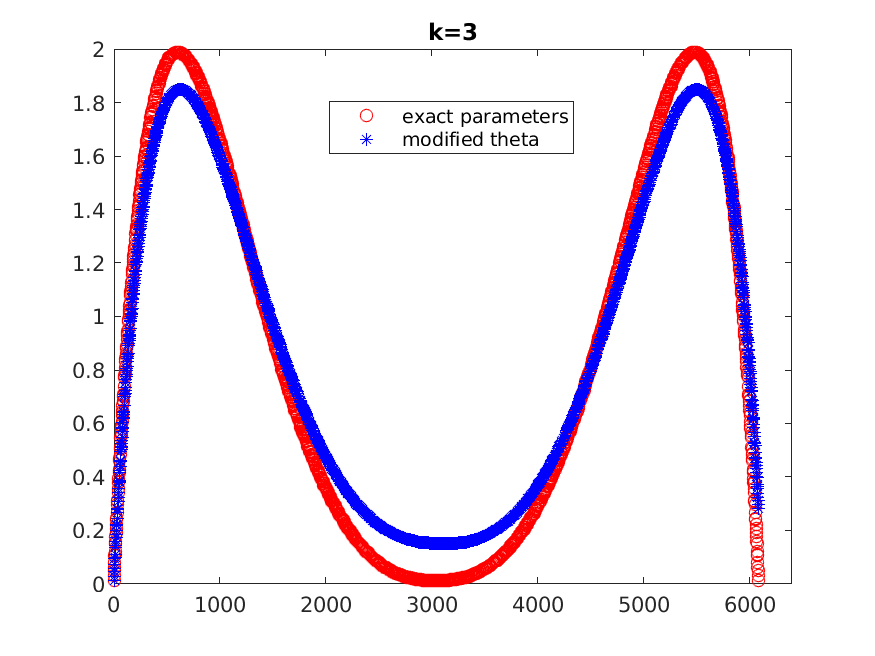
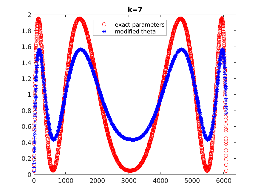
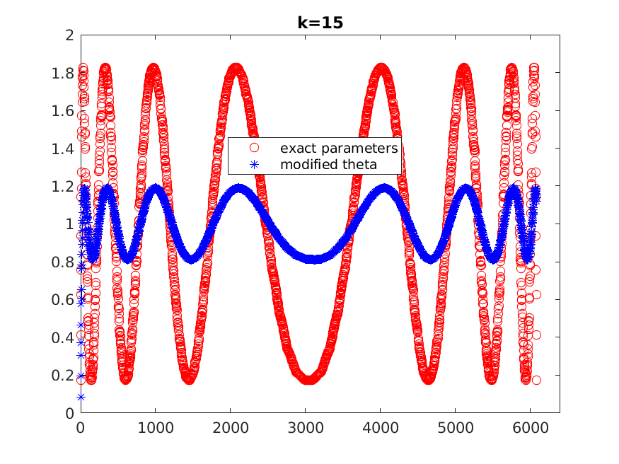
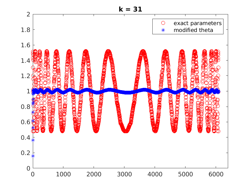
Fig. 2: Eigenvalue distribution of $P_{k}(A)A$ using the exact parameters (red circles) and modified $\theta$-value (blue stars) for different polynomial degrees

To clarify the situation we constructed the exact Chebyshev polynomials for the FD discretization of the Laplacian matrix in the unitary square of size 6084 whose exact eigenvalues are known. In Figure 2 we provide the eigenvalue distribution (red circles) of the preconditioned matrix $P_{k}(A)A,k=3,7,15,31.$ In the same picture we also provide the same plots, in which, however, the initial value of $\theta$ has been slightly modified by multiplying it by $1.01$ (the same result would have been obtained by reducing $\zeta_{0}=\dfrac{1}{\theta}$ in the Newton-based approach). The eigenvalue distribution is represented with blue stars in this case. The meaning of the figure is as follows: a circle/star with coordinate $(s,y)$ represents an eigenvalue of the preconditioned matrix $p_{k}(A)A$, namely $y=\lambda_{s}p_{k}(\lambda_{s})$, where $\lambda_{s}$ is the $s$-th eigenvalues of $A$ in increasing order.

Employing the Chebyshev preconditioner with exact parameters, the condition number is minimized but a clear clustering of the smallest eigenvalues is produced (see the bottom part of the red plots in Figure 2 and also Table 1, where the values of the indicator $l$, defined in (14), are shown). Slightly increasing the parameter $\theta$ yields an asymmetric spectrum of the preconditioned matrices which avoids clustering especially of the smallest eigenvalues which are very well separated. This behavior is known to speed-up the PCG convergence.

Table 1: PCG iterations for solving the $78^{2}$ discretized Laplacian in the unit square with polynomial preconditioner of degree $0,1,3,\ldots,31$. The extremal eigenvalues, the number $l$ of eigenvalues close to the minimum and the condition number of the preconditioned matrices are also reported.

	Original NC algorithm					NC with $\theta$ scaled by $1.01$
$m$	iter	$\mu_{\max}$	$\mu_{\min}$	$l$	$\kappa(P_{m}A)$	iter	$\mu_{\max}$	$\mu_{\min}$	$l$	$\kappa(P_{m}A)$
0	223	1.9992	7.9060e-04	1	2528.7	223	1.9794	7.8278e-04	1	2528.7
1	111	1.9968	3.1562e-03	2	632.7	112	1.9584	3.0647e-03	1	639.0
3	115	1.9875	1.2526e-02	188	158.7	61	1.8493	1.1318e-02	1	163.4
7	58	1.9514	4.8580e-02	278	40.2	31	1.5640	3.5202e-02	1	44.4
15	30	1.8268	1.7318e-01	468	10.5	17	1.1891	8.2247e-02	1	14.5
31	15	1.5193	4.8067e-01	874	3.2	11	1.0182	1.6060e-01	1	6.3

Indeed in Table 1 the reported results of the run for the polynomial preconditioners of degree $2^{j}-1,j=0,\ldots,5$ confirm that the scaling the Newton-Chebyshev polynomial preconditioner highly improves its performance as compared to using the optimal parameters. In the same Table we report the number of eigenvalues of the preconditioned matrix which are close to the minimum as

$$l=\#\left\{\lambda\,:\,\frac{\lambda}{\lambda_{\min}}<1.1\right\}.$$ (14)

With the scaled NC algorithm the smallest eigenvalue is isolated while with optimal parameters the number $l$ increases with the degree of the polynomial.

5 Numerical Results

We now report the results of numerical experiments to solve very large and sparse matrices, most of them arising from real engineering applications. In detail,

• Opt_Transp arises from the Finite Element discretization of the transient optimal transport problem Bergamaschi et al. (2019).

• Lap1600: is the Laplacian on the unitary square with $1598^{2}$ interior grid points.

• Cube_5317k: arises from the equilibrium of a concrete cube discretized by a regular unstructured tetrahedral grid.

• Emilia_923: arises from the regional geomechanical model of a deep hydrocarbon reservoir Ferronato et al. (2010). It is obtained discretizing the structural problem with tetrahedral Finite Elements. Due to the complex geometry of the geological formation it was not possible to obtain a computational grid characterized by regularly shaped elements.

The size and nonzero numbers of these problems are reported in Table 2.

Table 2: Size $n$, number of nonzeros nnz and spectral condition number $\kappa=\dfrac{\lambda_{n}}{\lambda_{1}}$ (computed after symmetric diagonal scaling) of the test matrices. Regarding matrix Opt_Trans the condition number has been computed as $\kappa=\dfrac{\lambda_{n}}{\lambda_{2}}$ since $\lambda_{1}=0$.

name	$n$	nnz	$\kappa(A)$
Opt_Trans	412417	2 882817	1.04 $\times 10^{6}$
Lap1600	2 553604	12 761628	2.42 $\times 10^{5}$
Emilia-923	923136	41 005206	3.08 $\times 10^{5}$
Cube${5317k}\$	5 317443	222 615369	3.30 $\times 10^{6}$

In the following results we will employ a polynomial of degree $m=2^{\rm nlev}-1$, with various values of the parameter nlev which also counts the Newton iterations. The scaling factor was set to $1.001$ for all problems. All matrices are preliminary diagonally scaled before solving the corresponding linear system. We consider as the exact solution a vector with all ones and computed the right hand side accordingly. Unless differently stated, we stop the PCG iteration as soon as the relative residual norm is below $\texttt{tol}=10^{-8}$.

5.1 Sequential tests

As common when dealing with polynomial preconditioners, the main issue is to cheaply assess the extremal eigenvalues. In the numerical results reported below we approximated $\beta_{0}$ with few iterations of the power method and $\alpha_{0}$ with the non preconditioned DACG method Bergamaschi et al. (1997) up to $10^{-2}$ tolerance on the relative residual. The sequential tests have been performed using Matlab on on an Intel Core 2 Quad at 3.50GHz, each core being equipped with 16Gb RAM.

The results reported in Table 3 refer to matrices Opt_Transp, Lap1600 and Cube${5317k}\$.

Table 3: Results of the NC polynomial preconditioner for matrices Opt_Transp, Lap1600 and Cube${5317k}\$for various degrees of the polynomial preconditioner. For the Cube${5317k}\$matrix the tolerance was set to $10^{-12}$.

	Matrix Opt_Transp					Matrix Lap1600			Matrix Cube${5317k}\$
$m$	iter	ddot	$A\times\mathbf{v}$	$\|\mathbf{r}_{k}\|/\|\mathbf{b}\|$	CPU(s)	iter	$\|\mathbf{r}_{k}\|/\|\mathbf{b}\|$	CPU(s)	iter	CPU(s)	$\|\mathbf{r}_{k}\|/\|\mathbf{b}\|$
0	3433	10299	3433	9.85e-09	26.39	4517	9.75e-09	203.52	9037	3040.0	9.94e-13
1	1773	5319	3536	9.70e-09	23.25	2313	9.99e-09	176.58	4604	2990.9	9.98e-13
3	879	2637	3516	9.92e-09	20.95	1174	9.87e-09	160.50	2413	3044.7	9.96e-13
7	439	1317	3512	8.85e-09	19.86	589	9.40e-09	151.79	1204	2999.6	9.52e-13
15	222	666	3552	8.39e-09	19.59	295	9.92e-09	147.83	604	2988.5	9.66e-13
31	117	351	3744	7.78e-09	20.33	149	9.50e-09	146.80	304	2996.9	9.97e-13
63	69	207	4416	5.49e-09	23.85	77	7.09e-09	151.17	156	3069.9	8.92e-13

Some comments are in order. The good news are that, apart from an obvious decrease of the number of scalar products:

1. Assessment of extremal eigenvalues is relatively cheap. It took only 0.69 seconds for the Opt_Transp matrix, 1.33 seconds for the Laplacian and $17.4$ seconds for the Cube${5317k}\$matrix.

2. The norm of the true residual at convergence decreases with $m$, confirming the improved conditioning of the preconditioned matrix.

3. The CPU time decreases by 15% – 25% by increasing the polynomial degree from $m=0$ to $m=15$. This does not hold for the matrix Cube${5317k}\$for which the cost of the matrix-vector products is predominant over the scalar products due to the high number of average nonzeros per row.

Remark. We do not claim that our polynomial preconditioner can compare favorably with other well-known sequential accelerators such as the Incomplete Cholesky preconditioner. We report, however, the performance of this preconditioner (as implemented by the Matlab function ICHOL($\delta$), $\delta$ being the drop tolerance) in combination with the CG solver for the three analyzed matrices. We also report the density of the Cholesky factor as $\rho=$ nonzero($L$)/nonzero($A$) (which is a measure of the increased storage demand of this preconditioner).

matrix	$\delta$	$\rho$	Iter	CPU
Lap1600	no fill	0.5	1344	151.02
Opt_Transp	$10^{-4}$	1.87	201	7.32
Cube${5317k}\$	$10^{-4}$	negative pivot encountered
Cube${5317k}\$	$10^{-5}$	out of memory

Number of iterations and CPU times are smaller than with the polynomial preconditioner, which, by contrast, does not require additional memory, is completely matrix free and easily parallelizable. Moreover we could not compute the IC factorization of the larger matrix Cube${5317k}\$due to memory limitations.

5.2 Numerical Results on a Parallel Platform

The polynomial preconditioner is based on matrix-vector products and no scalar products. This feature can be successively exploited on parallel architectures since, as known, when a high number of processors is employed, the dot product, being the only task that involves a collective communication, reveals a bottleneck for the parallel efficiency.

An efficient implementation of a parallel matrix vector product is obviously mandatory to achieve high parallel efficiency. In this paper we use an improved MPI-Fortran routine as successfully experimented in Martínez et al. (2009). We used a block row distribution of the coefficient matrix with complete consecutive rows assigned to different processors.

All tests have been performed on the new HPC Cluster Marconi at the CINECA Centre, on both the A1 version (1512 nodes, 2 $\times$ 18-cores Intel Xeon E5-2697 v4 (Broadwell) at 2.30 GHz) and the more recent A2 update (with 3600 nodes and 1$\times$ 68-cores Intel Xeon 7250 CPU (Knights Landing) at 1.4GHz). The Broadwell nodes have 128 Gb memory each, while in the A2 system the RAM is subdivided into 16GB of MDRAM and 96GB of DDR4. The Marconi Network type is: new Intel Omnipath, 100 Gb/s. (MARCONI is the largest Omnipath cluster of the world).

Throughout the whole section we will denote with $T_{\texttt{$p$}}$ the CPU elapsed times expressed in seconds (unless otherwise stated) when running the code on $p$ processors. We include a relative measure of the parallel efficiency achieved by the code. To this aim we will denote as $S_{\texttt{$p$}}^{(n_{0})}$, the pseudo speedup computed with respect to the smallest number of processors ($n_{0}$) used to solve the given problem:

$$S_{\texttt{$p$}}^{(n_{0})}=\frac{T_{n_{0}}\ n_{0}}{T_{\texttt{$p$}}}.$$

We will denote $E_{\texttt{$p$}}^{(n_{0})}$ the corresponding relative parallel efficiency, obtained according to

$$E_{\texttt{$p$}}^{(n_{0})}=\dfrac{S_{\texttt{$p$}}^{(n_{0})}}{\texttt{$p$}}=\frac{T_{n_{0}}\ n_{0}}{T_{\texttt{$p$}}{\texttt{$p$}}}.$$

Table 4: Scalability analysis for the Emilia-923 matrix.

	nlev $=5$			nlev $=2$			nlev $=0$
$p$	iter	$T_{p}$	$E_{p}^{(16)}$	iter	$T_{p}$	$E_{p}^{(16)}$	iter	$T_{p}$	$E_{p}^{(16)}$	$\dfrac{T_{p}(\texttt{lev}=0)}{T_{p}(\texttt{lev}=5)}$
16	379	114.44		3008	115.64		11386	117.15		1.02
64	379	33.33	86%	3008	34.43	84%	11382	37.74	78%	1.13
256	379	10.39	69%	3008	12.35	59%	11380	16.75	44%	1.61
512	379	6.15	58%	3008	9.15	39%	11380	14.70	25%	2.35

In Table 4 we report the scalability results for matrix Emilia-923 using levels $0,2$ and $5$ which correspond to using a polynomial preconditioner of degree $0$, $3$ and $31$, respectively. It is shown that the parallel efficiency is greatly improved when a high degree of the preconditioner is used. The relative efficiency from 16 to 1024 processors is increased from $25\%$ ($\text{lev}=0$) to $58\%$ ($\text{nlev}=5$) by a factor 2.35.

The scalability results for matrix Cube5317k, reported in Table 5 show a 1.6 CPU time reduction from nlev $=0$ to nlev $=5$.

Table 5: Scalability analysis for the Cube5317k matrix.

	nlev $=5$			nlev $=0$
$p$	iter	$T_{p}$	$E_{p}^{(64)}$	iter	$T_{p}$	$E_{p}^{(64)}$	$\dfrac{T_{p}(\texttt{nlev}=0)}{T_{p}(\texttt{nlev}=5)}$
64	298	154.79	–	9038	164.7	–	1.06
128	298	85.33	91%	9038	91.30	90%	1.07
256	298	46.60	83%	9038	53.63	77%	1.15
512	298	28.04	69%	9038	35.12	59%	1.25
1024	298	21.23	46%	9038	33.94	30%	1.60

The different parallel performance is related to the nonzero patterns of the two matrices. In matrix Cube5317k the nonzeros are more spread far from the diagonal (as a result of a local mesh refinement). This implies that a given processor must receive/send data with a large number of other processors when performing the matrix-vector product. This behavior is clearly shown in Figure 3. For the Cube5317k matrix the predominant parallel cost is represented by the matrix-vector product which is the bottleneck of the parallel computation for a high number of processors. Clearly, this unvaforable sparsity pattern can be improved by preprocessing the linear system with a suitable graph partitioning and fill-reducing matrix ordering. However we consider this test case, as it is, a worst case scenario for our preconditioner, which, however, is shown to obtain satisfactory speed-ups.

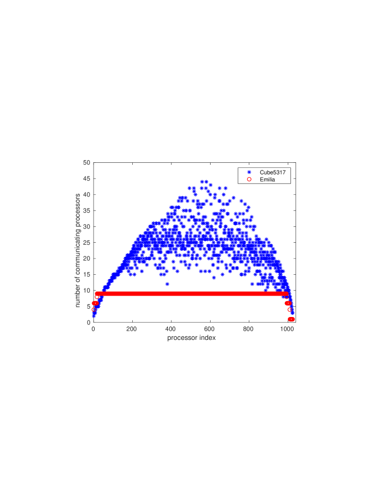
Fig. 3: Number of communicating processors with a given processor in performing the matrix-vector product. Matrices Cube5317k and Emilia-923 with $p$ = 1024.

5.3 Results on huge matrices

We now report the results in solving huge linear systems arising from Finite Difference (FD) 3D discretization of the Poisson equation in the unitary cube. These last runs have been conducted on the new Marconi 100 supercomputer available at Cineca. MARCONI 100 is the new accelerated cluster based on 980 IBM Nodes, each equipped with 2x16 cores IBM POWER9 AC922 at 3.1 GHz processors.

We consider three very large matrices: lap3d(nx), where $\texttt{nx}=512,1024,2048$ is the number of subdivisions in each spatial dimension. The size, nonzeros and condition number of these matrices are reported in Table 6.

Table 6: Size $n$, number of nonzeros nnz and condition number $\kappa$ for the 3 FD-3D matrices.

nx	$n$	nnz	$\kappa(A)$
512	$1.3\times 10^{8}$	$9.4\times 10^{9}$	$1.06\times 10^{5}$
1024	$1.1\times 10^{9}$	$7.5\times 10^{9}$	$4.24\times 10^{5}$
2148	$8.6\times 10^{9}$	$6.0\times 10^{10}$	$1.70\times 10^{6}$

Table 7: CPU times and iterations for the FD-3D(nx) problems for various degree of the polynomial and varying number of processors.

nx	$p$	nlev $=5$		nlev $=2$		nlev $=0$		$\dfrac{T_{p}(\texttt{nlev}=0)}{T_{p}(\texttt{nlev}=5)}$
		iter	$T_{p}$	iter	$T_{p}$	iter	$T_{p}$
512	64	45	67.0	325	67.4	1300	95.3	1.4
	128	45	36.2	325	38.1	1300	50.2	1.4
	256	45	21.8	325	21.8	1300	27.7	1.3
	512	45	13.8	325	13.3	1300	16.8	1.3
1024	64	88	858.4	637	945.2	2553	1481.7	1.7
	256	88	254.3	637	284.3	2553	400.6	1.6
	1024	88	97.2	637	101.6	2553	131.5	1.4
2048	512	165	1925.7	–	–	5033	3169.8	1.6
	2048	165	710.5	–	–	5033	1001.5	1.4

The results, reported in Table 7, show that we are able to solve very huge size problems with a good (relative) strong scalability. Moreover the polynomial preconditioner (either with nlev $=2$ or nlev = $5$) takes from 1.3 to 1.7 less CPU time than the diagonal preconditioner.

On the huge problem lap3d(2048) the relative efficiency from 512 to 2048 processors is around $70\%$. This problem, with eight billion unknowns and 56 billion nonzeros has been solved with 165 iterations, three times as many scalar products, and 710.5 seconds with 2048 processors.

Weak scalability analysis. We finally perform a sort of weak scalability analysis, weighted by taking into account that the condition number, and hence the number of PCG iterations, grows with nx. In detail, doubling the nx parameter the size of the corresponding matrix increases by a factor 8; moreover its condition number increases by a factor 4 and therefore the PCG iteration number is expected to roughly double. Summarizing, from a matrix to the subsequent one in the sequence, we may expect an increase of a factor 16 in the CPU time (with constant number of processors). Defining as $T_{nx,\texttt{$p$}}$ the CPU time needed to solve a FD-3D matrix with nx and $p$ processors a perfect weak scalability would predict a dependence of the CPU time on nx and $p$ as

$$T_{\texttt{nx},\texttt{$p$}}=O\left(\frac{\texttt{nx}^{4}}{p}\right)$$

from which, assuming now $\texttt{$p$}=\texttt{nx}$:

$$T_{2\texttt{$p$},2\texttt{$p$}}=8T_{\texttt{$p$},\texttt{$p$}}=64T_{\frac{\texttt{$p$}}{2},\frac{\texttt{$p$}}{2}}.$$

From Table 7 we have indeed that, for nlev = $0$, $\dfrac{T_{2048,2048}}{T_{512,512}}=59.6$ whereas for nlev = $5$ $\dfrac{T_{2048,2048}}{T_{512,512}}=51.5$, which are both smaller (and hence better) than the theoretically optimal value of 64.

5.4 Comparisons with other parallel preconditioners

The proposed preconditioner has many pleasant features such as: No additional memory requirements, No need to explicitly store the matrix, It takes the number of scalar products to a very low value. To show that it is also convenient in terms of overall efficiency we carried out a comparison with a state-of-the-art parallel preconditioned solver for SPD linear system. It is the solver chronos, available at the webpage https://www.m3eweb.it/chronos/, which makes use of an enhanced AMG solver, partially based on a FSAI smoother with dynamical nonzero pattern selection Franceschini et al. (2019); Paludetto Magri et al. (2019)

In Table 8 we reported the results in solving the FD matrix with $nx=512$ for the PCG method accelerated with either the AMG or the FSAI preconditioners, after some trials to select the optimal parameters. Since the setup time to evaluate the preconditioner is rather high for this approach we reported this in the table as $T_{\text{setup}}$ while the CPU time for the PCG solution is $T_{\text{solver}}$. $T_{p}=T_{\text{setup}}+T_{\text{solver}}$ is, as before, the overall CPU time.

Table 8: Results for the solution of the FD-3D problem with $nx=512$ using the chronos package.

	AMG preconditioner				FSAI preconditioner
	with FSAI as smoother
$p$	iter	$T_{\text{setup}}$	$T_{\text{solver}}$	$T_{p}$		$T_{\text{setup}}$	$T_{\text{solver}}$	$T_{p}$
64	23	21.5	10.8	32.3	786	5.9	86.4	92.4
128	24	15.3	7.1	22.4	774	2.7	43.7	46.5
256	26	12.4	4.4	16.8	782	1.7	24.4	26.2
512	28	14.3	4.6	18.8	758	0.7	13.8	14.5

Inspection of Tables 8 and 7 reveals that our polynomial preconditioner compares very well with this state-of-the-art solver both in terms of scalability and CPU times. Regarding the PCG solution times only, the AMG approach outperforms the NC preconditioner, however the gap progressively reduces as the number of processors increases.

6 Conclusions

We have proposed a (potentially high-degree) polynomial preconditioner for the Conjugate Gradient method with the aim of greatly reducing the number of scalar products which may represent a bottleneck especially in parallel computations. By avoiding clustering of extremal eigenvalues, the preconditioner obtains its best performances when the degree $m$ is relatively high (good results have been obtained with $m=31$ or $m=63$). Numerical results onto very large matrices reveal that these polynomial preconditioners may be successfully employed to accelerate the Conjugate Gradient method by drastically reducing the number of scalar products (and hence the collective communications in parallel environments). In sequential computations the polynomial preconditioner with degree $31$ reduces the CPU time of about $30\%$ with respect to the diagonal preconditioner. Parallel runs with up to 2048 processors on the Marconi supercomputer show that the important reduction in the number of scalar products (which reduces roughly to 97% smaller with respect to the diagonal preconditioner, with $m=31$) yielding a improvement over the diagonal preconditioner from 30% to 60% of the total CPU time.

Further study is undergoing to give theoretical setting how to compute the optimal scaling parameter. Moreover, a low-rank acceleration of the polynomial preconditioner will be investigated, following e.g. Bergamaschi (2020) by exploiting the well separation of the smallest eigenvalues provided by our polynomial preconditioner. We finally observe that the described approach can be applied whenever a first level parallel preconditioner is at hand in factored form, say $P_{0}=WW^{T}$, to obtain a second level preconditioner applying the Newton-Chebyshev polynomials to the matrix $W^{T}AW$.

Acknowledgements

This work was partially supported by the Project granted by the CARIPARO foundation Matrix-Free Preconditioners for Large-Scale Convex Constrained Optimization Problems (PRECOOP) and by the INdAM Research group GNCS, 2020 Project: Optimization and advanced linear algebra for problems arising from PDEs.

References

- Benzi et al. (2000) M. Benzi, J. K. Cullum, and M. Tůma. Robust approximate inverse preconditioning for the conjugate gradient method. SIAM J. Sci. Comput., 22(4):1318–1332, 2000. ISSN 1064-8275. URL https://doi.org/10.1137/S1064827599356900.
- Bergamaschi (2020) L. Bergamaschi. A survey of low-rank updates of preconditioners for sequences of symmetric linear systems. Algorithms, 34 (2)(100), 2020.
- Bergamaschi et al. (1997) L. Bergamaschi, G. Gambolati, and G. Pini. Asymptotic convergence of conjugate gradient methods for the partial symmetric eigenproblem. Numer. Linear Algebra Appl., 4(2):69–84, 1997.
- Bergamaschi et al. (2019) L. Bergamaschi, E. Facca, A. Martínez, and M. Putti. Spectral preconditioners for the efficient numerical solution of a continuous branched transport model. J. Comput. Applied Math., 254:259–270, 2019.
- Chen (2005) K. Chen. Matrix preconditioning techniques and applications, volume 19 of Cambridge Monographs on Applied and Computational Mathematics. Cambridge University Press, Cambridge, 2005. URL https://doi.org/10.1017/CBO9780511543258.
- Cheney (1966) E. W. Cheney. Introduction to approximation theory. McGraw-Hill Book Co., New York, 1966.
- Embree et al. (2018) M. Embree, J. A. Loe, and R. B. Morgan. Polynomial preconditioned Arnoldi. arXiv: 1806.08020, math.NA, 2018.
- Ferronato et al. (2010) M. Ferronato, G. Gambolati, C. Janna, and P. Teatini. Geomechanical issues of anthropogenic co2 sequestration in exploited gas fields. Energy Conversion and Management, 51(10):1918 – 1928, 2010. ISSN 0196-8904.
- Franceschini et al. (2019) A. Franceschini, V. A. Paludetto Magri, G. Mazzucco, N. Spiezia, and C. Janna. A robust adaptive algebraic multigrid linear solver for structural mechanics. Computer Methods in Applied Mechanics and Engineering, (352):389–416, 2019.
- Hotelling (1943) H. Hotelling. Some new methods in matrix calculation. Ann. Math. Statist., 14(1):1–34, 03 1943. 10.1214/aoms/1177731489. URL https://doi.org/10.1214/aoms/1177731489.
- Johnson et al. (1983) O. G. Johnson, C. A. Micchelli, and G. Paul. Polynomial preconditioners for conjugate gradient calculations. SIAM J. Numer. Anal., 20(2):362–376, 1983. ISSN 0036-1429. 10.1137/0720025. URL https://doi.org/10.1137/0720025.
- Kaporin (2012) I. E. Kaporin. Using Chebyshev polynomials and approximate inverse triangular factorizations for preconditioning the conjugate gradient method. Computational Mathematics and Mathematical Physics, 52(2):169 – 193, 2012.
- Loe and Morgan (2019) J. A. Loe and R. B. Morgan. New polynomial preconditioned GMRES. arXiv: 1911.07065, math.NA, 2019.
- Loe et al. (2019) J. A. Loe, H. K. Thornquist, and E. G. Boman. Polynomial preconditioned GMRES to reduce communication in parallel computing. arXiv: 1907.00072, math.NA, 2019.
- Martínez et al. (2009) A. Martínez, L. Bergamaschi, M. Caliari, and M. Vianello. A massively parallel exponential integrator for advection-diffusion models. J. Comput. Applied Math., 231(1):82–91, 2009.
- Paludetto Magri et al. (2019) V. A. Paludetto Magri, A. Franceschini, and C. Janna. A novel amg approach based on adaptive smoothing and prolongation for ill-conditioned systems. SIAM Journal of Scientific Computing, (41):A190–A219, 2019.
- Saad (1985) Y. Saad. Practical use of polynomial preconditionings for the conjugate gradient method. SIAM Journal on Scientific and Statistical Computing, 6(4):865–881, 1985. 10.1137/0906059. URL https://doi.org/10.1137/0906059.
- Saad (2003) Y. Saad. Iterative Methods for Sparse Linear Systems. Second edition. SIAM, Philadelphia, PA, 2003.
- Saad and Schultz (1986) Y. Saad and M. H. Schultz. GMRES: A generalized minimal residual algorithm for solving nonsymmetric linear systems. SIAM J. Sci. Stat. Comput., 7(3):856–869, 1986.
- Świrydowicz et al. (2020) K. Świrydowicz, J. Langou, S. Ananthan, U. Yang, and S. Thomas. Low synchronization gram-schmidt and generalized minimal residual algorithms. Numerical Linear Algebra with Applications, page e2343, 2020. https://doi.org/10.1002/nla.2343. published online 22 Oct, 2020.
- van Gijzen (1995) M. B. van Gijzen. A polynomial preconditioner for the GMRES algorithm. Journal of Computational and Applied Mathematics, 59(1):91 – 107, 1995.