The Dwarf Planet Makemake as seen by X-Shooter

Abstract

Makemake is one of the brightest known trans-Neptunian objects, as such, it has been widely observed. Nevertheless, its visible to near-infrared spectrum has not been completely observed in medium resolving power, aimed at studying in detail the absorption features of CH₄ ice. In this paper we present the spectrum of Makemake observed with X-Shooter at the Very Large Telescope (Chile). We analyse the detected features, measuring their location and depth. Furthermore, we compare Makemake’s spectrum with that of Eris, obtained with the same instrument and similar setup, to conclude that the bands of the CH₄ ice in both objects show similar shifts.

1 Introduction

(136472) Makemake (just Makemake in the remaining of the text) is one of the largest trans-Neptunian objects (TNOs), having an equivalent diameter of ($1,430\pm 9$) km and a visible albedo of $(0.77\pm 0.03)$ (Ortiz et al., 2012). Its rotational period is estimated as $(22.8266\pm 0.001)$ h, double peaked light-curve, with a peak-to-peak amplitude of $(0.032\pm 0.005)$ mags (Hromakina et al., 2019), in contrast to the value of $(7.7710\pm 0.0030)$ h (single peaked light-curve) reported by Heinze & DeLahunta (2009).

Recently, Parker et al. (2016) reported the detection of a satellite about 8 magnitudes fainter than Makemake, whose orbit remains yet to be determined. This orbit will allow to measure the mass of Makemake and, therefore, its density, which can be contrasted to different values in the literature: $(1.7\pm 0.3)$ gcm^-3 from Ortiz et al. (2012), > 1.98 gcm^-3 from Brown (2013), or $\lesssim 1.8$ gcm^-3 estimated by Bierson & Nimmo (2019). Noteworthy, Hromakina et al. (2019) also suggested the existence of a second satellite, close to the primary, whose existence remains to be confirmed.

The visible to near-infrared (VNIR) spectrum of Makemake is dominated by absorption bands of CH₄ ice (Licandro et al., 2006). Their central positions are very close to the ones of pure CH₄ ice measured on laboratory, but still slightly blue-shifted, which seem to indicate that Makemake is one the objects with largest amount of CH₄ ice on its surface. These shifts are attributed to the mixture of ices: CH₄ and possibly N₂ in different levels of dilution (for instance, see Quirico & Schmitt, 1997; Brunetto et al., 2008; Protopapa et al., 2015). For the sake of comparison, Pluto (Merlin et al., 2010, and references therein) presents large blue-shifts (usually > 10 Å) in the spectral signatures of CH₄, interpreted as larger dilutions of CH₄ in N₂. Although other ices might be present on the surface of Makemake, for instance CO, as observed in Pluto, its effect might be negligible (Tan & Kargel, 2018).

Several authors have presented VNIR spectroscopy of Makemake, measuring the position and depth of the CH₄ absorption features (for example Licandro et al., 2006; Tegler et al., 2007, 2008; Lorenzi et al., 2015; Perna et al., 2017). The deep and broad absorption features (see Fig. 1) are interpreted in terms of very large slabs formed by sintering (Eluszkiewicz et al., 2007). The small blue-shifts of the absorption features are in agreement with the Schaller & Brown (2007) (updated in Brown, 2012) model of volatile retention that shows Makemake on the border of N₂ ice retention region. Nevertheless, this model should be interpreted with care because it only gives an upper limit on the survivability of the ices, furthermore, the Jeans escape rate has been shown to be even smaller than expected for Pluto’s atmosphere (see Young et al., 2020, and references therein).

Most of the measurements of the relative position of the CH₄ ice bands of Makemake were performed in the visible range $(\lambda<0.9$ $\mu$m) with resolving power usually $\leq 1,000$, with a few exceptions, e.g., $\sim 1,400$ in Tegler et al. (2008) and about 3,000 in Perna et al. (2017). Before continuing it is important to mention that the resolving power is the ability of a spectrograph to resolve a spectral line of width at half maximum $\delta\lambda$ at a wavelength $\lambda$ and is given by $R=\lambda/\delta\lambda$. In the NIR, most of the published spectra have $R<100$, with the exception of Brown et al. (2015)’s with $R\sim 2,500$. Due to the usually low resolving power of the NIR spectra, it is not possible to carry on detailed studies of absorption features above 1.0 $\mu$m. To stress the importance of mid-resolving power NIR spectroscopy ($1,000\lesssim R\lesssim 10,000$), Brown et al. (2015) showed that irradiation products of CH₄ ice, for instance C₂H₆ ice, improve the spectral modelling of Makemake, especially for $\lambda>1.6$ $\mu$m. Therefore, in this work we present mid-resolving power spectrum of Makemake ($R>4,000$) in a large spectral range. The spectrum was obtained with X-Shooter @ Very Large Telescope (VLT) and it has the highest SNR obtained so far simultaneously in the VNIR range.

This work is organised as follows, in the next section we describe the observations and data reduction. In Sect. 3 we show our results, while in Sect. 4 we present the discussion and in Sect. 5 the conclusions drawn from this work.

2 Observations and data reduction

Makemake was observed in service mode using X-Shooter, attached to the Cassegrain focus of the unit 2 of the VLT (Cerro Paranal, Chile) on April 26, 2013. X-Shooter is an echelle spectrograph able to obtain at once a complete spectrum between 0.35 and 2.4 $\mu$m. The incoming beam of light is split using two dichroic beam splitters and redirected into three arms: UVB ($0.35-0.55$ $\mu$m), VIS ($0.55-1.0$ $\mu$m), and NIR ($1.0-2.4$ $\mu$m). Each arm works as an independent spectrograph recording a different part of the spectrum.

We used the instrumental setup shown in Table 1. In the NIR arm we selected a restricted mode that only records the spectrum up to 1.8 $\mu$m, while everything above is blocked out. The blocked region shows a very strong thermal contamination that damages the signal for faint objects, even contaminating the H region. Using this setup we obtain an increased efficiency in the $1.5-1.8$ $\mu$m region. The observations were taken nodding on the slit following a standard ABBA pattern.

Table 1: Observational Circumstances

Object	Arm	Read Out Mode / binning	Slit (arcsec)	Exptime (s)	Airmass
	UVB	100 khz / $1\times 2$	1.0	$4\times 480$
Makemake	VIS	100 khz / $1\times 2$	0.9	$4\times 500$	1.761
	NIR	Non Destructive Mode	0.9	$4\times 480$
	UVB	100 khz / $1\times 2$	1.0	$2\times 0.7$
HD89010	VIS	100 khz / $1\times 2$	0.9	$2\times 0.7$	1.550
	NIR	Non Destructive Mode	0.9	$2\times 0.7$

We used the star HD89010, a.k.a. 35 Leo, of spectral type G1.5IV-V, to remove the solar signature from Makemake’s spectrum and as telluric star (see Table 1).

The data were delivered via ftp package including all necessary calibration files and reduced using the X-Shooter pipeline version 2.0.0, which handles the whole reduction process: BIAS or DARK correction, whichever is necessary, FLAT-FIELDING, order identification, rectification of the raw spectra, wavelength calibration, sky-subtraction, and merging of the orders into, first, a two-dimensional image, and then into a one-dimensional spectrum. We did not use this last spectrum, opting to make our own extraction form the 2D image using apall.iraf. This ensures a better control over the final signal-to-noise ratio of the spectrum.

After extraction of the spectra we divided the spectrum of Makemake by that of the star removing the solar signature and correcting most of the telluric absorption due to Earth’s atmosphere, obtaining our final reflectance spectrum. Finally, we normalised it to unity at 0.55 $\mu$m.

2.1 Filtering

The resulting reflectance spectrum is still noisy, which makes it difficult to detect where an absorption feature starts and where it ends. It also has many remaining bad pixels that were not flagged during the pipeline processing. We decided to filter the spectrum using wavelets, in particular the family of wavelets Coiflet as they showed an optimal behaviour in comparison with other families of wavelets (see Souza-Feliciano et al., 2018). We also chose to work with wavelets instead of other filtering techniques, such as re-binning, running box, or Fourier analysis because it revealed as the technique that better respected the input signal (Souza-Feliciano et al., 2018).

Wavelets de-construct the signal into two parts: one principal and one residual. The deconvolution occurs simultaneously in the spatial and frequency domains (Starck & Murtagh, 2006). We used scale of 2 because we only wanted to remove bad pixels. We used the hard-filtering that removes coefficients below a certain threshold, respecting the shape of the features.

Figure 1 shows the spectrum of Makemake after the process (bottom spectrum). It is possible to see a few remaining bad pixels, which occur at the joint of the different echelle orders, especially in the VIS arm. We decided to not go further with the cleaning process to avoid the destruction of real features of the spectrum. We also discarded the region below 0.4 $\mu$m because it was too noisy to be reliable.

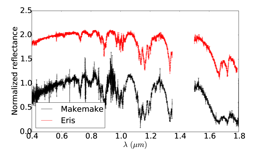
Figure 1: Spectra of Makemake, in black, and Eris, in red. Both spectra are normalised to 0.55 $\mu$m, while Eris’ was shifted in the y-scale for clarity. The region between 1.4 and 1.5 $\mu$m was removed due to strong atmospheric absorption. Both spectra were obtained with X-Shooter.

We will use this spectrum in the remaining of the work.

3 Results

In this work we will use as comparison a spectrum of Eris obtained also with X-Shooter because we aim to compare spectra of similar resolving power, obtained with the same instrument. The details of Eris’ observation and data reduction can be found in Alvarez-Candal et al. (2011). Note that the spectrum of Eris was de-noised in the same way as described above. To make the most of the resolving power of our spectrum we will analyse first the characteristics of the absorption features, i.e., band depth ($D$) and wavelength shifts ($\Delta\lambda$), and then look into the possible surface composition.

3.1 Spectrum in the visible

An important characteristic of the spectrum is its colour in the visible range. Therefore, we first compared the visible spectral slope, $S^{\prime}$, using the CANA package (De Pra et al., 2018), that fits a linear function between 0.4 and 0.52 $\mu$m and estimates this parameter. The spectral slope measured for Makemake is $S_{M}^{\prime}=(21.2\pm 0.6$) $\%/1000$ Å and for Eris is $S_{E}^{\prime}=(13.5\pm 0.2$) $\%/1000$ Å. Notice that these values are not to be directly compared with others in the literature (for instance Lorenzi et al., 2016) because these values are dependent of the exact definition used for $S^{\prime}$, which changes from work to work.

A direct comparison can be made using $(B-V)$ and $(V-R)$ colours. We used the transmission curves, $T(\lambda)$, of the three filters to weight the spectra and obtain relative magnitudes, which were then transformed into standard magnitudes using solar colours (from Ramírez et al., 2012) following

$$(M_{1}-M_{2})_{\rm obj}=-2.5\log{(f_{1}/f_{2})}+({M_{1}-M_{2}})_{\odot},$$

where

$$f_{i}=\frac{\int{T_{i}(\lambda})flux(\lambda)d\lambda}{\int{T_{i}(\lambda})d\lambda},~{}i=B,V,R.$$

We obtained, for Makemake, $(B-V)=0.868\pm 0.004$ and $(V-R)=0.449\pm 0.003$, while for Eris $(B-V)=0.782\pm 0.003$ and $(V-R)=0.393\pm 0.003$. These values are in agreement with those reported in the MBOSS database by Hainaut et al. (2012): $(B-V)=0.84\pm 0.02$ and $(V-R)=0.48\pm 0.02$ for Makemake, and $(B-V)=0.78\pm 0.03$ and $(V-R)=0.39\pm 0.05$ for Eris.

The most accepted hypothesis to explain the red colours of Makemake and Eris is the existence of complex organics molecules (tholins) formed from simple organics by photolysis (e.g. Simonia & Cruikshank, 2018; Khare et al., 1984). A possible explanation for the difference could be that Eris has less tholins than Makemake.

3.1.1 Subtle features

Besides the clear absorption features mentioned in Table 2, Tegler et al. (2007) reported the detection of small bands located at 0.54, 0.58, and 0.6 $\mu$m. Our spectrum of Makemake only shows a hint of an absorption at 0.54 $\mu$m with a depth of about 2 %, barely marginal over the point-to-point variation of the spectrum, and therefore unreliable, while none of the other features could be detected (see Fig. 2).

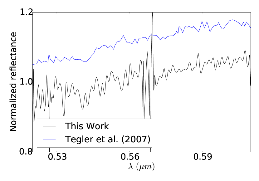
Figure 2: Comparison between spectra of Makemake zoomed to the 0.52 $\mu$m and 0.61 $\mu$m. Both were normalised to unite at 0.55 $\mu$m, Tegler et al.’s is shifted by 0.1 in the y-axis for clarity.

3.2 Wavelength shifts

We measured wavelength shifts ($\Delta\lambda$, expressed in Å) and depths ($D$, expressed in %) of the spectral features detected on the spectrum of Makemake by comparison with the spectrum of CH₄ ice obtained in laboratory. We analysed one by one several of the absorption features seen in Fig. 1 with the following procedure: (i) We determine a linear continuum around the shoulders of the band of interest and divide the spectrum by this continuum. (ii) We select a small window around the apparent minimum of the feature and fit a second degree polynomial. The position of the minimum is taken as the zero of the first derivative of the polynomial. (iii) The process is repeated 10,000 times each time modifying the normalised flux values within a normal distribution with width equal to the nominal error at that wavelength. The final position is taken as the average value and its error of the flux as the standard deviation. (iv) To compute $D$ we used the weighed average flux, $f_{w}$, within the same window via

$$D~{}[\%]=\big{(}1-f_{w}^{-1}\big{)}\times 100.$$ (1)

(v) The positions of the CH₄ ice absorption bands are similarly measured. Note that, in this stage, we do not try to fit a specific model to the band of Makemake (or Eris). Instead, we use several models of CH₄ ice at 40 K (Grundy et al., 2002) for different grain sizes. We remove the local continuum in the same way as for our objects’ data and define a small window around the minimum of the band. We fit a second degree polynomial within the window for all the models and choose the band position as the average and its error as the standard deviation. (vi) We obtain

$$\Delta\lambda=\lambda_{\rm object}-\lambda_{\rm reference}.$$

Values of $\Delta\lambda$ and $D$ for Makemake and Eris are shown in Table 2 and displayed in Figs. 3 and 4 as function of wavelength.

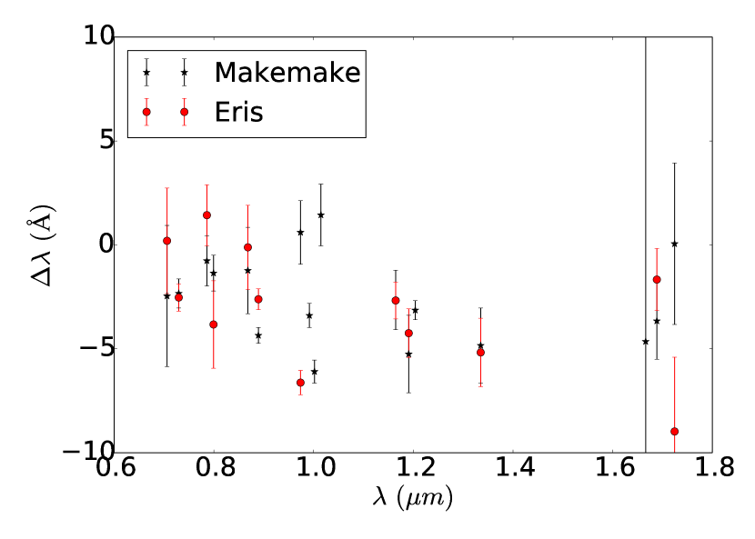
Figure 3: $\Delta\lambda$ vs. $\lambda$ for Makemake (black stars) and Eris (red circles).

Table 2: Wavelength shifts and band depths. The first column shows the nominal central wavelength of the band, the second and third columns show the results for Makemake, the fourth and fifth for Eris, white the last columns shows the difference between Makemake and Eris.

CH4	Makemake		Eris		M-E
$\lambda$ ($\mu$m)	$\Delta\lambda$ (Å)	$D$ (%)	$\Delta\lambda$ (Å)	$D$ (%)	$\Delta\lambda$ (Å)
0.62		12.4 (0.5)		5.2 (0.2)	1.7 (3.0)
0.71	-2.5 (3.4)	7.1 (0.3)	0.2 (4.2)	3.2 (0.1)	-2.7 (4.2)
0.73	-2.3 (0.7)	32.1 (1.5)	-2.5 (1.0)	16.2 (0.7)	0.2 (1.0)
0.79	-0.8 (1.2)	8.2 (0.3)	1.4 (1.9)	5.1 (0.1)	-2.2 (1.9)
0.80	-1.4 (0.9)	9.8 (0.4)	-3.8 (2.3)	4.8 (0.2)	2.5 (2.3)
0.87	-1.2 (2.1)	24.1 (1.5)	-0.1 (2.9)	14.9 (0.7)	-1.1 (2.9)
0.89	-4.4 (0.4)	37.4 (2.2)	-2.6 (0.4)	31.4 (0.7)	-1.7 (0.4)
0.97	0.6 (1.5)	28.2 (2.1)	-6.6 (1.6)	17.7 (0.9)	7.2 (1.6)
0.99	-3.4 (0.6)	31.7 (2.2)
1.00	-6.1 (0.6)	23.0 (2.0)
1.01	1.4 (1.5)	31.7 (1.4)
1.16	-2.6 (1.4)	55.9 (0.8)	-2.7 (1.7)	57.7 (1.2)	0.0 (1.7)
1.19	-5.3 (1.9)	35.0 (0.7)	-4.2 (2.2)	29.3 (0.5)	-1.0 (2.2)
1.20	-3.1 (0.5)	28.3 (3.6)
1.33	-4.8 (1.8)	44.1 (1.4)	-5.2 (1.3)	62.1 (3.4)	0.3 (1.3)
1.67	-4.6 (30.6)	49.2 (3.5)		62.7 (7.4)
1.69	-3.7 (1.8)	16.2 (1.3)	-1.7 (1.4)	23.2 (0.2)	-2.0 (1.4)
1.72	0.1 (3.9)	42.2 (2.0)	-9.0 (1.6)	62.5 (6.6)	9.0 (1.6)
Average	-2.6 (2.1)		-3.1 (2.8)		0.8 (3.5)

In Fig. 3 it is apparent that Makemake follows a similar trend as already seen for Eris in Alvarez-Candal et al. (2011). We have not included in this work other comparisons, as done in our previous work, because our intent was to compare data of similar quality, wavelength coverage, and resolving power.

Figure 4 shows $D$ vs. $\lambda$.

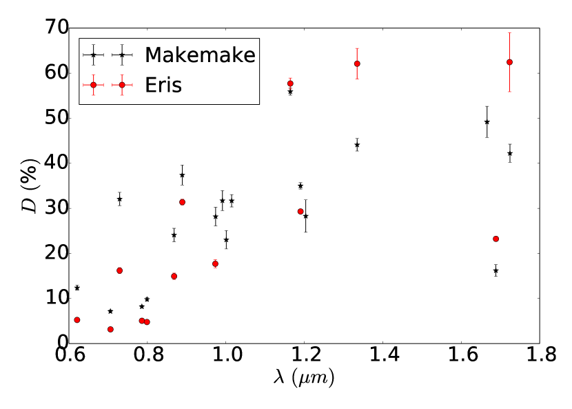
Figure 4: $D$ vs. $\lambda$ for Makemake (black stars) and Eris (red circles).

Makemake tends to have deeper absorption bands than Eris, with the exception of the region beyond 1.4 $\mu$m where the bands of Makemake are strongly saturated (except the 1.68 $\mu$m band) and, therefore, their depth becomes unreliable as, once saturated, the feature cannot grow deeper, instead its width increases. Deeper absorption features appear towards longer wavelength, which as pointed in many works (for instance Alvarez-Candal et al., 2011, and references therein) could be related to the thickness of the layer. Therefore, in Fig. 5 we report the change of $\Delta\lambda$ with respect to $D$. It is possible to see that there is a small increase in the blue-shift with increasing depth, noticeable both on Makemake and Eris. To test this hypothesis we ran the Spearman test on both sets of data. The anti-correlation has a marginal statistically significance in the case of Eris, with a correlation parameter $r_{s}=-0.66$ and significance over $2\sigma$. No correlation is significant in the case of Makemake.

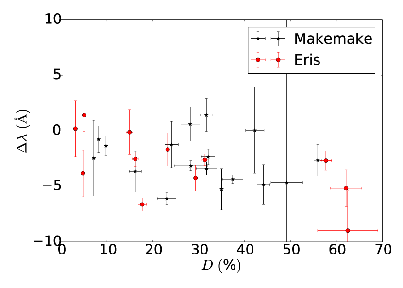
Figure 5: $\Delta\lambda$ vs. $D$ for Makemake (black stars) and Eris (red circles).

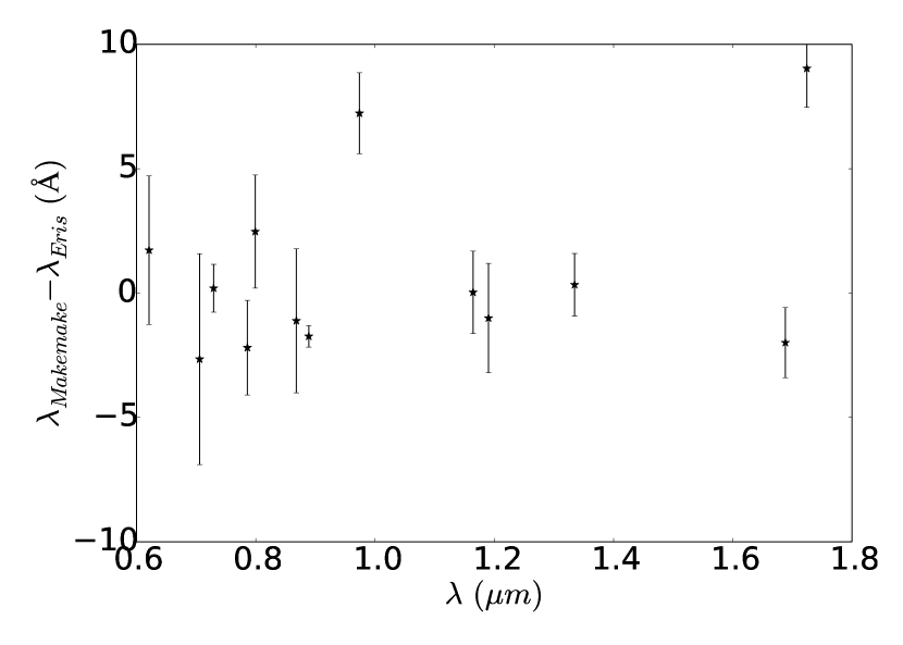
Figure 6: $\Delta\lambda$ vs. $\lambda$, comparison between Makemake and Eris.

In the case of Eris we proposed that this could be indicative of a collapsed atmosphere onto its surface, could it be the same for Makemake? It seems difficult, because of its size and location which, in principle, preclude the existence of large quantities of volatile ices other than CH₄ on its surface.

Noteworthy is the remarkable fact that most of the $\Delta\lambda$ measured for Makemake and Eris are quite similar (Fig. 6 and Table 2). The absorption features are mostly within three standard deviations from $\Delta\lambda=0$ Å. We ran a 2 sample Kolmogorov-Smirnov test on the two sets, obtaining that we cannot reject the hypothesis that both $\Delta\lambda$-distributions come from the same parent distribution, with a significance over $2\sigma$. This, certainly, does not mean that the surfaces of Makemake and Eris are identical.

3.2.1 Cross-Correlation experiment

Aiming at double-checking our results from the previous section, we applied the cross-correlation function (Brockwell & Davis, 2009), CCF, to obtain the most likely shift between Makemake and CH₄ ice. We compute the errors of the shift from the confidence interval based on a Marquardt-Levemberg Algorithm (Levenberg, 1944; Marquardt, 1963). We also obtain a more conservative error from a Monte Carlo Markov Chain, MCMC, of $10,000$ nodes with $25$% of acceptance (Foreman-Mackey et al., 2013).

We applied shifts from $-25$ to $25$ steps in resolution bin of the spectra to obtain a measurement of the covariance between the Makemake spectra and the ice. We fit a second-degree polynomial to find the centre of the CCF, that corresponds to the maximum covariance and, therefore, to the most likely shift. We obtain the maximum CCF based on the Nelder-Mead Algorithm (Nelder & Mead, 1965). We use the shift from Nelder-Mead to obtain the confidence intervals based on Marquardt-Levemberg Non-Linear Least Squares algorithm and the MCMC.

The shift between Makemake and CH₄ is $-1.38\pm 0.03$ Å, with a more conservative result of $-1.38\pm 3.38$ Å (Fig. 7). We also applied the cross-correlation analysis between Makemake and Eris. The shift with Eris is $-0.11\pm 0.02$ Å, and assuming a conservative statistics, the shift is $-0.11\pm 3.59$ Å (Fig. 8). The shift between Makemake and Eris is smaller than the variation in wavelength from each point in the resolution of Makemake spectra, which is $\Delta\lambda=0.19$ Å. In Table 3 are summarised the results of the cross-correlation experiments. These values are compatible with the averages shown in Table 2.

Table 3: Wavelength shifts from Cross-Validation Function between Makemake with our model, and Makemake with Eris.

Algorithm	$\Delta\lambda$ from Ice	$\Delta\lambda$ from Eris
	Å	Å
Nelder-Mead	$-1.38$	$-0.11$
Marquardt-Levemberg	$-1.38\pm 0.03$	$-0.11\pm 0.02$
MCMC	$-1.38\pm 3.38$	$-0.11\pm 3.59$

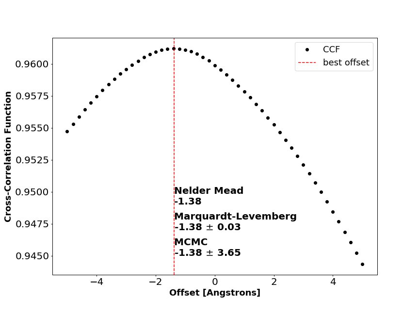
Figure 7: Makemake offset from Ice.

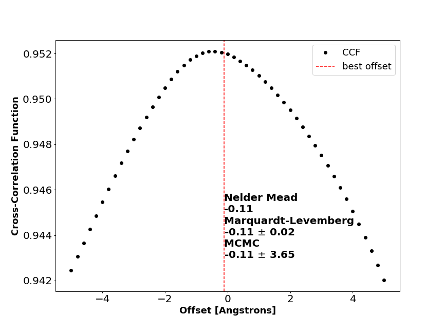
Figure 8: Makemake offset from Eris.

3.3 Spectral Modelling

We created synthetic spectra of Makemake and Eris using the Hapke radiative transfer model (Hapke, 1993) with optical constants of pure CH₄ ice at 40 K (Grundy et al., 2002). Other scattering theories exist (e.g., Douté & Schmitt, 1998; Shkuratov et al., 1999) that could provide similar quality of fits to the data as those presented here, but with different percentages and grain sizes of the components (Poulet et al., 2002). However, we decided to interpret our data with a simple model since it provides a reasonable fit to both spectra and we are not aiming at a detailed description of their surface composition, which has been extensively studied elsewhere (see references in the Sect. 1). Because our goal is to perform a comparative study between Makemake and Eris we only use different combinations of pure CH₄ ice. Also, the synthetic spectra are limited to $\lambda>0.7$ $\mu$m.

For the purpose of this work, we assumed that CH₄ ice is spatially segregated on the surfaces of Makemake and Eris. The model that best fits the spectrum of Makemake contains 50% of CH₄ ice of 1 cm grains, 30% of 2 cm grains, and 20% with grains of 0.1 cm (Fig. 9). The model provides a close description of the data. However, there are some remaining differences, especially in the 1.5 to 1.7 $\mu$m range. The spectral model of Eris (Fig. 10) contains 60% of CH₄ ice with grains of 0.3 cm, 30% with 0.2 cm grains, and 10% with grains of 0.1 cm. With exception of the spectral range between 1.5 to 1.7 $\mu$m, where apparently an extra absorption is needed, the model describes the properties of the reflectance of the surface satisfactorily.

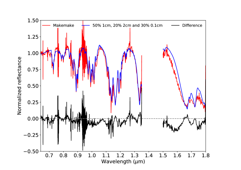
Figure 9: Normalised spectrum of Makemake (red) compared with a synthetic spectra (blue) made with different proportions and size grains of CH₄ (see the text). The difference between the original and synthetic spectra is shown in black. The region close to 1.4 $\mu$m was masked due to the absorption of the atmosphere.

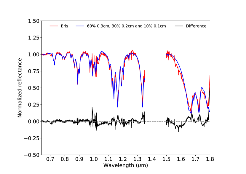
Figure 10: Normalised spectrum of Eris (red) compared with a synthetic spectra (blue) made with different proportions and size grains of CH₄ (see the text). The difference between the original and synthetic spectra is shown in black. The region close to 1.4 $\mu$m was masked due to the absorption of the atmosphere.

3.4 NIR spectrum interpretation

The optical properties of the spectra of Makemake and Eris are dominated by CH₄ ice. In the case of Eris, its radius ($1,163\pm 6$ km, Sicardy et al., 2011) and temperature about 35 K (Sicardy et al., 2011) support the retention of volatile ices (Schaller & Brown, 2007), however no direct detection other than CH₄ has been possible to date. In particular N₂ or CO ices might be found, but the low temperature keeps these ices in their $\alpha$-state, whose spectral features cannot be resolved by X-Shooter (see Alvarez-Candal et al., 2011). On the other hand, considering Makemake’s size ($\sim 1400$ km) and surface temperature [36 K, if it were a slow rotator (see Ortiz et al., 2012, supplemental information)], the retention regime for this object is different than the retention regime for Eris (Brown, 2012). Makemake is capable of retaining CH₄ ice but is not expected to retain large amounts of N₂ or CO ices, so their direct detection in its near-infrared spectrum is unlikely (Brown et al., 2007).

The molecule of CH₄ ice is optically very active, therefore, the presence of other components are masked by its absorption bands. Nevertheless, Eris’ and Makemake’s CH₄ bands are seen to be partially shifted to shorter wavelengths relative to the wavelengths of pure CH₄ ice absorption bands (see Sect.3.2), indicating that CH₄ and N₂ are present on Eris and Makemake.

4 Discussion

Our spectrum of Makemake does not confirm the detection of the subtle absorption bands of CH₄ ice short-ward of 0.62 $\mu$m proposed by Tegler et al. (2007). One possible explanation is the lower SNR of our spectrum, although with a larger resolving power. Nevertheless, it must be kept in mind that these bands are expected to exist (e.g., Patel et al., 1980), but they would be extremely hard to detect due to the large path lengths necessary to produce them.

As mentioned in the Introduction, neither Lorenzi et al. (2015) nor Perna et al. (2017) detected any significant heterogeneity on the surface of Makemake. Both works used rotational resolved spectroscopy with good resolving power in the visible part. Unfortunately, we do not have rotational resolved spectra of Makemake, but we do cover a wider spectral range with higher resolving power. Our data show that the centres of the absorption features of CH₄ ice seen on the spectra of Makemake and Eris have remarkably similar blue-shifts, when compared with CH₄ ice measured in laboratory. Furthermore, Makemake’s band centres are marginally bluer than Eris’, which seemed a priori unlikely because Eris should have retained more volatile ices than Makemake due to its size and location, and it is unexpected (e.g. Young et al., 2020, pg 130). Nevertheless, if the N₂ is in different phases, that might explain, at least partially these shifts. In Quirico & Schmitt (1997), the shifts of the features of CH₄ ice are slightly larger if the N₂ ice is in its $\alpha$-phase, as expected for Eris. Interestingly, Makemake follows a similar trend in the $\Delta\lambda$ vs. $D$ space as Eris: deeper adsorptions show larger shifts, although with less statistical significance. We do not believe this is pointing to a collapsed frozen atmosphere on the surface of Makemake, but rather to the scatter of our data.

The spectral slope in the visible range of Makemake is larger than the Eris, suggesting that more processed material is in fact present on the surface of Makemake. The rough spectral modelling performed on both spectra show large residuals (Figs. 9 and 10), especially in the $1.5-1.7$ $\mu$m. We attribute these differences to minor components on the surface of these objects, as proposed by Brown et al. (2015). They showed that high-order hydrocarbons are present in the spectrum of Makemake, in particular ethane (C₂H₆), that improve the modelling of the spectrum (see Perna et al., 2017).

5 Conclusions

In this work we present X-Shooter data of the dwarf planet Makemake which, to the best of our knowledge, has the greater resolving power over a large spectral range. The spectrum is compared with that of CH₄ ice and that of Eris, obtained with the same instrument and similar observational setup.

The modelling of the spectrum shows the need for more ingredients besides pure CH₄ ice, not only for the large residuals, but also for the location of the absorption bands. Interestingly, we see that the location of the features in Makemake and Eris are remarkably similar. Furthermore, Makemake’s are slightly blue-shifted, with respect to Eris’, instead of red-shifted, as it was usually expected. This could only be achieved with mid-resolving power spectroscopy.

The wavelength shifts could be affected by the reservoir of volatile on the surface of both dwarf-planets and by the temperature of their surfaces over their orbits, especially in the passages by their perihelia. Furthermore, the temperature is key in the phase of the N₂ ice, which experiences the transition from $\alpha$ to $\beta$ phase at 35.6 K. The low-temperature $\alpha$-phase ice has much deeper and narrower absorption bands and is likely to be the dominant phase of N₂ at Eris (Alvarez-Candal et al., 2011), whereas, Makemake’s with higher surface temperature, and closer to the Sun, is more likely to contain the $\beta$-phase of N₂ ice. The fact that the shifts of the bands, for both Makemake and Eris, are larger for the deepest bands is an indicative that the mixture of CH₄ and N₂ must be more abundant in the subsurface layers so, while the surface of Eris could be covered by a richer N₂ layer, product of the collapse of an atmosphere, Makemake, because of its redder colour, would be richer in the products of the irradiation of CH₄, the tholins. What is the actual nature of these tholins is something that JWST will be able to investigate, same as for the presence of the lower temperature N2-ice, never directly detected in the solar system before.

Data Availability

The data underlying this article will be shared on reasonable request to the corresponding author.

References

- Alvarez-Candal et al. (2011) Alvarez-Candal A., et al., 2011, A&A, 532, A130
- Bierson & Nimmo (2019) Bierson C. J., Nimmo F., 2019, Icarus, 326, 10
- Brockwell & Davis (2009) Brockwell P. J., Davis R. A., 2009, Time Series: Theory and Methods (Springer Series in Statistics). Springer
- Brown (2012) Brown M. E., 2012, Annual Review of Earth and Planetary Sciences, 40, 467
- Brown (2013) Brown M. E., 2013, The Astrophysical Journal, 767, L7
- Brown et al. (2007) Brown M. E., Barkume K. M., Blake G. A., Schaller E. L., Rabinowitz D. L., Roe H. G., Trujillo C. A., 2007, The Astronomical Journal, 133, 284
- Brown et al. (2015) Brown M. E., Schaller E. L., Blake G. A., 2015, The Astronomical Journal, 149, 105
- Brunetto et al. (2008) Brunetto R., Caniglia G., Baratta G. A., Palumbo M. E., 2008, ApJ, 686, 1480
- De Pra et al. (2018) De Pra M., Carvano J., Morate D., Licandro J., Pinilla-Alonso N., 2018.
- Douté & Schmitt (1998) Douté S., Schmitt B., 1998, J. Geophys. Res., 103, 31367
- Eluszkiewicz et al. (2007) Eluszkiewicz J., Cady-Pereira K., Brown M. E., Stansberry J. A., 2007, Journal of Geophysical Research, 112, E06003
- Foreman-Mackey et al. (2013) Foreman-Mackey D., Hogg D. W., Lang D., Goodman J., 2013, PASP, 125, 306
- Grundy et al. (2002) Grundy W. M., Schmitt B., Quirico E., 2002, Icarus, 155, 486
- Hainaut et al. (2012) Hainaut O. R., Boehnhardt H., Protopapa S., 2012, A&A, 546, A115
- Hapke (1993) Hapke B., 1993, Theory of reflectance and emittance spectroscopy
- Heinze & DeLahunta (2009) Heinze A. N., DeLahunta D., 2009, The Astronomical Journal, 138, 428
- Hromakina et al. (2019) Hromakina T. A., et al., 2019, A&A, 625, A46
- Hunter (2007) Hunter J. D., 2007, Computing In Science & Engineering, 9, 90
- Khare et al. (1984) Khare B., Sagan C., Arakawa E., Suits F., Callcott T., Williams M., 1984, Icarus, 60, 127
- Levenberg (1944) Levenberg K., 1944, Quarterly of Applied Mathematics, 2, 164
- Licandro et al. (2006) Licandro J., Pinilla-Alonso N., Pedani M., Oliva E., Tozzi G. P., Grundy W. M., 2006, Astronomy & Astrophysics, 445, L35
- Lorenzi et al. (2015) Lorenzi V., Pinilla-Alonso N., Licandro J., 2015, Astronomy & Astrophysics, 577, A86
- Lorenzi et al. (2016) Lorenzi V., Pinilla-Alonso N., Licandro J., Cruikshank D. P., Grundy W. M., Binzel R. P., Emery J. P., 2016, A&A, 585, A131
- Marquardt (1963) Marquardt D. W., 1963, Journal of the Society for Industrial and Applied Mathematics, 11, 431
- Merlin et al. (2010) Merlin F., Barucci M. A., de Bergh C., DeMeo F. E., Alvarez-Candal A., Dumas C., Cruikshank D. P., 2010, Icarus, 210, 930
- Nelder & Mead (1965) Nelder J. A., Mead R., 1965, The Computer Journal, 7, 308
- Ortiz et al. (2012) Ortiz J. L., et al., 2012, Nature, 491, 566
- Parker et al. (2016) Parker A. H., Buie M. W., Grundy W. M., Noll K. S., 2016, The Astrophysical Journal, 825, L9
- Patel et al. (1980) Patel C. K. N., Nelson E. T., Kerl R. J., 1980, Nature, 286, 368
- Perna et al. (2017) Perna D., Hromakina T., Merlin F., Ieva S., Fornasier S., Belskaya I., Mazzotta Epifani E., 2017, Monthly Notices of the Royal Astronomical Society, 466, 3594
- Poulet et al. (2002) Poulet F., Cuzzi J., Cruikshank D., Roush T., Dalle Ore C., 2002, Icarus, 160, 313
- Protopapa et al. (2015) Protopapa S., Grundy W. M., Tegler S. C., Bergonio J. M., 2015, Icarus, 253, 179
- Quirico & Schmitt (1997) Quirico E., Schmitt B., 1997, Icarus, 127, 354
- Ramírez et al. (2012) Ramírez I., et al., 2012, ApJ, 752, 5
- Schaller & Brown (2007) Schaller E. L., Brown M. E., 2007, The Astrophysical Journal, 659, L61
- Shkuratov et al. (1999) Shkuratov Y., Starukhina L., Hoffmann H., Arnold G., 1999, Icarus, 137, 235
- Sicardy et al. (2011) Sicardy B., et al., 2011, Nature, 478, 493
- Simonia & Cruikshank (2018) Simonia I., Cruikshank D. P., 2018, Open Astronomy, 27, 341
- Souza-Feliciano et al. (2018) Souza-Feliciano A. C., Alvarez-Candal A., Jiménez-Teja Y., 2018, A&A, 614, A92
- Starck & Murtagh (2006) Starck J.-L., Murtagh F., 2006, Astronomical Image and Data Analysis, doi:10.1007/978-3-540-33025-7.
- Tan & Kargel (2018) Tan S. P., Kargel J. S., 2018, MNRAS, 474, 4254
- Tegler et al. (2007) Tegler S. C., Grundy W. M., Romanishin W., Consolmagno G. J., Mogren K., Vilas F., 2007, The Astronomical Journal, 133, 526
- Tegler et al. (2008) Tegler S. C., Grundy W. M., Vilas F., Romanishin W., Cornelison D. M., Consolmagno G. J., 2008, Icarus, 195, 844
- Young et al. (2020) Young L. A., Braga-Ribas F., Johnson R. E., 2020, in Prialnik D., Barucci M. A., Young L. A., eds, , The Trans-Neptunian Solar System. Elsevier, pp 127 – 151, doi:https://doi.org/10.1016/B978-0-12-816490-7.00006-0, http://www.sciencedirect.com/science/article/pii/B9780128164907000060