Quantifying uncertainty and dynamical changes in multi-species fishing mortality rates, catches and biomass by combining state-space and mechanistic multi-species models

Abstract

In marine management, fish stocks are often managed on a stock-by-stock basis using single-species models. Many of these models are based upon statistical techniques and are good at assessing the current state and making short-term predictions; however, as they do not model interactions between stocks, they lack predictive power on longer timescales. Additionally, there are mechanistic multi-species models that represent key biological processes and consider interactions between stocks such as predation and competition for resources. Due to the complexity of these models, they are difficult to fit to data, and so many mechanistic multi-species models depend upon single-species models where they exist, or ad hoc assumptions when they don’t, for parameters such as annual fishing mortality.

In this paper we demonstrate that by taking a state-space approach, many of the uncertain parameters can be treated dynamically, allowing us to fit, with quantifiable uncertainty, mechanistic multi-species models directly to data. We demonstrate this by fitting uncertain parameters, including annual fishing mortality, of a size-based multi-species model of the Celtic Sea, for species with and without single-species stock-assessments. Consequently, errors in the single-species models no longer propagate through the multi-species model and underlying assumptions are more transparent.

Building mechanistic multi-species models that are internally consistent, with quantifiable uncertainty, will improve their credibility and utility for management. This may lead to their uptake by being either used to corroborate single-species models; directly in the advice process to make predictions into the future; or used to provide a new way of managing data-limited stocks.

Running title: Uncertainty in multi-species models

Keywords: Bayesian Statistics; MCMC; Mechanistic models; Multi-species modelling; Uncertainty quantification; State-space approach;

1 Introduction

Food security has been highlighted as one of the major global challenges, with fisheries and aquaculture identified as key contributors to addressing this challenge (FAO, 2009; Frid & Paramor, 2012). Currently the majority of fish stocks are managed using single-species models (SSMs), such as the state-space assessment model (SAM) (Nielsen & Berg, 2014) and projections are made to assess the utility of management decisions. Interacting stocks, which may compete with or predate on one another, can make conventional single-species management difficult (Tyrrell et al., 2011; Quárou & Tomini, 2013; Farcas & Rossberg, 2016). Alternatively a multi-species or whole ecosystem approach could be adopted to account for these interactions (Pikitch et al., 2004; Link et al., 2011; Plagányi et al., 2014). There are several multi-species models (MSMs) ranging from statistical models (e.g. Stochastic MSM (SMS) Lewy & Vinther, 2004), to more mechanistic-based models (e.g. mizer; Scott et al., 2014) or whole ecosystem models (e.g. StrathE2E; Heath, 2012).

SSMs and statistical MSMs are often used to describe the current and recent status of the system, and to make short-term forecasts. They aim to learn about the system by fitting many ‘tuning parameters’, parameters that are adjusted to make the model look like the observed system (Plagányi et al., 2014; Brynjarsdóttir & O’Hagan, 2014). On the other hand, mechanistic models, sometimes called process-based models, are based on the theoretical understanding of the relevant ecological processes (Cuddington et al., 2013). They generally model the behaviour of the system through differential equations and/or a series of rules or algorithms. They prioritise realism over reality, often explaining why things happen rather than describing what happened (White & Marshall, 2019). Many of the parameters are treated as ‘input variables’, with values taken from other sources (Brynjarsdóttir & O’Hagan, 2014), leaving fewer ‘tuning parameters’ that represent processes that are either too complex or not known, e.g. recruitment. For example, in mechanistic size-based MSMs, the predator-prey mass ratio is an ‘input variable’, coming from other studies (e.g. Hatton et al., 2015), whereas in statistical MSMs it is treated as a ‘tuning parameter’ and learned from data (e.g. ICES, 2017a) (see Supplementary material S5 for an illustrative example of ‘tuning parameters’ and ‘input variables’). As mechanisms and physical laws are time invariant and more robust than statistical correlations, mechanistic models are better at predicting outside the immediate domain in which they were fitted, such as in the future (Connor et al., 2017; Cuddington et al., 2013).

Often mechanistic MSMs are fitted to, or rely on inputs from, SSMs (e.g. Blanchard et al., 2014; Mackinson et al., 2018). A common example is instantaneous fishing mortality values that are taken from SSMs, to drive fishing dynamics in MSMs (e.g. Spence et al., 2016; Speirs et al., 2016). In some ecoregions, fishing mortality values from SSMs either do not exist for all species or only qualitative patterns are reported. In studies with MSMs, fishing dynamics for species without fishing mortality values from SSMs are added using ad hoc methods (Thorpe et al., 2015). Further, as models are simplifications of reality and often the fishing mortality is treated as a ‘tuning parameter’, the fishing mortality values lose their interpretation outside of the fitted model (Rougier & Beven, 2013). Thus they are not the same as the true instantaneous fishing mortality values but instead are model specific. For example statistical MSMs, that are often used to generate natural mortality values for SSMs, have different fishing mortality than the SSMs (e.g. North Sea Cod in SMS and SAM; ICES, 2017a, 2018b), despite being fitted to the same data and having a similar representation of the population structure. Fitting MSMs to SSMs or taking inputs from them can lead to circularity in results as errors propagate through the models (Brooks & Deroba, 2015).

In MSMs, fitting fishing can be a challenging task. Recent software advances (e.g. ADMB (Fournier et al., 2012)) have meant that statistical MSMs, designed with tractability in mind, are relatively easy to fit. For mechanistic-based MSMs, fitting using traditional methods can be a difficult task. Evaluating the output of a model for a particular set of inputs can often be done only by running the model, which can take anything from a few seconds to a few hours. This means that fitting a large number of uncertain parameters, such as fitting fishing mortality for each year, can be a difficult task. Furthermore, for these models to be any use to support management, outputs need to be reported with robust estimates of uncertainty (Harwood & Stokes, 2003).

Parameter uncertainty has previously been explored in MSMs to explore a handful of parameters (Thorpe et al., 2015; Mackinson et al., 2018). Spence et al. (2016) fitted a size-based model of the North Sea using a Bayesian framework, which we adopt here (Bayes, 1763), using Markov chain Monte Carlo (MCMC) to sample from the posterior distribution (Metropolis et al., 1953; Hastings, 1970). Adding dynamical parameters, such as annual fishing mortality, makes the uncertain parameter space very large, making it difficult to explore. However, we may be able to consider the model as a state-space model, a common approach in SSMs (see Aeberhard et al., 2018, for a recent review). In state-space models, the ‘state’ of the system is updated using a Markov process, known as the process model, and there are some noisy, possibly incomplete, observations of the ‘state’, defined by an observation model. State-space models have a specific dependence structure (see Figure 1), with the observations of the past and present being conditionally independent given the unobserved state, a structure that can be advantageous when fitting the model (Zucchini et al., 2016).

There are many methods of fitting non-linear state-space models including Extended Kalman Filers (Evensen, 2003; Wan & Van Der Merwe, 2000), MCMC methods (Jonsen et al., 2005) and using the Laplace approximation (Tierney & Kadane, 1986) to integrate out the unobserved states (Skaug & Fournier, 2006). Spence et al. (2018) used particle filters (Gordon et al., 1993; Liu & Chen, 1998) to update a few years of fishing rates in two MSMs, but for longer periods of time this method is not practical. This is due to the likelihood being largely dominated by the process model and not the observation model which leads to poor mixing of the MCMC (Fasiolo et al., 2016). In this paper we develop an MCMC algorithm that sequentially updates each dynamical parameter and improves the mixing of the MCMC.

In many cases the only way of evaluating the likelihood of parameter values is to run the model. Running mechanistic models can be slow so ideally one would want to parallelise the model when fitting to data; however this is difficult for MCMC, as iterations need to be done sequentially (Jacob et al., 2011). Some MCMC algorithms have been developed that take advantage of parallel computing (Cui et al., 2011; Calderhead, 2014), whereas others reduce the number of times that the model needs to be run. The delayed-acceptance MCMC algorithm (Sherlock et al., 2017) uses a fast approximation of the likelihood, possibly using a statistical model, before deciding whether or not to run the mechanistic model. Due to the high dimensionality of this problem, fitting accurate fast approximations of the likelihood can be difficult, but for many of these problems there are some parameters that affect only part of the likelihood. Here we introduce a second new MCMC algorithm that runs several proposals in parallel using the mechanistic model and then combines them to give a single proposal that has an increased chance of being accepted.

In this paper we fit fishing mortality and other uncertain parameters of a multi-species size-based model for the Celtic Sea, without the use of SSMs. We compare stock-assessments made using the MSM with those developed using SSMs. Although demonstrated on a multi-species marine model, this problem is not unique to MSMs and methods demonstrated here can be used for fitting mechanistic-based models of intermediate complexity, e.g. individual-based models (Railsback & Grimm, 2011), especially when there are dynamic parameters. In Section 2 we define state-space models, describe the multi-species size-based model, the data and the fitting procedure as well as the two new MCMC algorithms. In Section 3 we describe the results of the fitted model and we conclude with a discussion in Section 4. We also demonstrate the fitting procedure with a simulation study using another mechanistic MSM (Spence et al., 2020b) in the Simulation study.

2 Methods

In this section we describe how we can treat the MSM as a state-space model. We introduce the MSM used in this study, the uncertain parameters, which include fishing mortality for each species for each year, and the data to which the model was fitted. We then describe the steps used to sample from the posterior distribution using Markov Chain Monte Carlo (MCMC).

2.1 State-space model

Let ${M}_{t}$ be the state of the MSM at time $t$. Then

$${M}_{t}|{M}_{t-1}\sim h({M}_{t-1},\bm{\phi}_{t},\bm{\theta}),$$

where $\bm{\phi}_{t}$ are dynamical parameters at time $t$ and $\bm{\theta}$ are static parameters. $h(\cdot)$ is known as the process model. We do not observe the state directly but at time $t$ we observe $\bm{y}_{t}$, where

$$\bm{y}_{t}|{M}_{t}\sim{}g({M}_{t},\bm{\sigma}^{2}),$$

and $\bm{\sigma}^{2}$ are static parameters. $g(\cdot)$ is known as the observation model. Figure 1 represents this model as a directed acyclic graph (DAG).

Figure 1: A directed acyclic graph of the state-space model.

Process model

The process model $h(\cdot)$ used here is the deterministic multi-species size-based model, mizer (Hartvig et al., 2011; Scott et al., 2014), and the state of the model, $M_{t}$, is a collection of the density of all species, $N_{i}(m)$, and the background resource, $N_{R}(m)$ at all weights, $m$ at time $t$ (see Supplementary material S1 for details). Mizer was developed to represent the size and abundance of all organisms from zooplankton to large fish predators in a size-structured food web. Some species are represented by species-specific traits and body size while others are represented solely by body size. The core of the model involves ontogenetic feeding and growth, mortality, and reproduction driven by size-dependent predation and maturation processes. The smallest individuals in the model do not eat fish belonging to the fish populations, but consume smaller planktonic or benthic organisms which we describe as a background resource spectrum. Fish grow and die according to size-dependent predation and, if mature, recruit new young which are put back into the system at the minimum weight. As well as the predation and background mortality, the fish in the model also experience fishing mortality.

In this study we fit mizer for 17 species, shown in Table 1, in the Celtic Sea, ICES (International Council for Exploration of the Seas) areas 7e-j. A description of the model can be found in the Supplementary material (S1) along with the parameter values.

In mizer there are a number of uncertain parameters to estimate. The carrying capacity of the background resource spectrum, $\kappa$, is uncertain, with a relatively uninformative prior distribution given by $\ln(\kappa)\in[0,40]$ uniformly (see Table 2). Recruitment follows a density-dependent process with the maximum number of recruits of the $i$th species being $R_{max,i}$, which is also uncertain. We specified a relatively uninformative prior distribution as $\ln(R_{max,i})\in[0,50]$ uniformly (see Table 2), for all $i$. The fishing mortality of the $i$th species of weight $m$ at time $t$ was

$$\phi_{t,i}q_{i}(m),$$

where $q_{i}(m)$ is the catchability of species $i$ at size $m$, normalised so that $\max_{m}(q_{i}(m))=1$, and $\phi_{t,i}$ is the fishing rate (values for $q_{i}(m)$ are shown in the Supplementary material (Figure S1)). The model was run from 1991-2014 ($t=1,\ldots,24$) and the fishing rate for each species for each year was also uncertain with $\phi_{t,i}\in[0,1.5]$ uniformly for $t=1,\ldots,24$ and for all $i$.

The model can be sensitive to its initial state, when $t=0$, and so the model was projected for 300 years to a stationary state, a process known as spin-up, with a fixed fishing rate $\phi_{0,i}$ for each species prior to running for $t=1,\ldots,24$. As in Spence et al. (2016) we treated the spin-up fishing rates as additional parameters with $\phi_{0,i}\in[0,1.5]$ uniformly for all $i$ (see Table 2). We consider $\bm{\theta}=(\ln\kappa,\ln{}R_{max,1:17},\phi_{0,1:17})^{\prime}$ to be ‘static’ parameters and the fishing rates, $\phi_{1:24,1:17}$ to be ‘dynamical’ parameters (with $1{:}17$ meaning $i=1\ldots 17$).

In addition to the commercial fishing mortality, we included survey fishing mortality. The catchability of the survey vessel was taken from Walker et al. (2017) and the fishing effort for the survey effort taken from DATRAS (ICES, 2017b). By including the survey fishing mortality we are able to fit the model to data from survey.

Table 1: The species in the Celtic Sea mizer model

$i$	Common name	Latin name
1	Atlantic herring	Clupea harengus
2	European sprat	Sprattus sprattus
3	Atlantic cod	Gadus morhua
4	Haddock	Melanogrammus aeglefinus
5	Whiting	Merlangius merlangus
6	Blue whiting	Micromesistius poutassou
7	Norway pout	Trisopterus esmarkii
8	Poor cod	Trisopterus minutus
9	European hake	Merluccius merluccius
10	Monkfish	Lophius piscatorius
11	Atlantic horse mackerel	Trachurus trachurus
12	Atlantic mackerel	Scomber scombrus
13	Common dab	Limanda limanda
14	European Plaice	Pleuronectes platessa
15	Megrim	Lepidorhombus whiffiagonis
16	Common sole	Solea solea
17	Boarfish	Capros aper

Table 2: The uncertain parameters.

Parameters	Dimensions	Units	Prior	Notes
$\ln{R_{max,1:17}}$	17	$\ln(vol^{-1}grams^{-1}year^{-1})$	$U(0,50)$	Natural log of the maximum recruitment
				for each species
$\ln{\kappa}$	1	$\ln(grams^{-\lambda-1}vol^{-1})$	$U(0,40)$	Natural log of the carrying capacity
				of the resource spectrum
$\phi_{0,1:17}$	17	$year^{-1}$	$U(0,1.5)$	The fishing rates during the spin-up
				period for each species
$\phi_{1:24,1:17}$	$17\times 24=408$	$year^{-1}$	$U(0,1.5)$	The fishing rate for each species
				for each year
$\sigma^{2}_{s,1:17}$	17	Unitless	$Inv-Gamma(2,2)$	The variance of the error on
				the natural log survey catches
$\sigma^{2}_{c,1:17}$	17	Unitless	$Inv-Gamma(0.1,0.1)$	The variance of the error on
				the natural log commercial catches

Observation model

At time $t$, we observe catches in tonnes, $\bm{y}$, made up of those by commercial vessels, $\bm{w}_{t}$ for $t=1,\ldots{},24$ (1991-2014), and those by the International Bottom Trawl Survey (IBTS), $\bm{z}_{t}$ for $t=7,\ldots{},24$ (1997-2014), with $|\bm{w}_{t}|=|\bm{z}_{t}|=17$. We take

$$\ln\bm{w}_{t}\sim{}N(\ln{\bm{c}(M_{t})},\Sigma_{c})$$

where $\bm{c}(M_{t})$ is the commercial catch from the process model and $\Sigma_{c}$ is a diagonal matrix with elements $\bm{\sigma}_{c}^{2}$. Similarly we take

$$\ln\bm{z}_{t}\sim{}N(\ln{\bm{s}(M_{t})},\Sigma_{s})$$

where $\bm{s}(M_{t})$ is the survey catch from the process model and $\Sigma_{s}$ is a diagonal matrix with elements $\bm{\sigma}_{s}^{2}$. The $i$th elements of $\bm{c}(M_{t})$ and $\bm{s}(M_{t})$ are denoted ${c}(M_{t})_{i}$ and ${s}(M_{t})_{i}$ and defined in equations S3 and S4 in the Supplementary material respectively. The likelihood of the model is

$$l(\bm{y}|\bm{\theta},\phi_{1:24,1:17},\bm{\sigma}_{c}^{2},\bm{\sigma}_{s}^{2}) = \prod_{i=1}^{17}\prod_{t=1}^{24}N(\ln(w_{t,i})|\ln(c(M_{t})_{i}),\sigma_{c,i}^{2})$$ (1)

$$\quad\times\prod_{t=7}^{24}N(\ln(z_{t,i})|\ln(s(M_{t})_{i}),\sigma_{s,i}^{2}),$$

where $w_{t,i}$, $z_{t,i}$, $\sigma_{c,i}^{2}$ and $\sigma_{s,i}^{2}$ are the $i$th element of $\bm{w}_{t}$, $\bm{z}_{t}$, $\bm{\sigma}_{c}^{2}$ and $\bm{\sigma}_{s}^{2}$ respectively, and $N(a|d,e)$ is a normal density with expectation $d$ and variance $e$ evaluated at $a$. Table 2 summarises the uncertain parameters.

2.2 Data

Landings data were extracted from ICES (ICES, 2017c) and discards were estimated as a percentage of the retained biomass (Heymans et al., 2016; Anon, 2015). All discards were assumed to have been removed from the living stock in the process model, such that all discards are assumed to have died. As only discards and no landings were recorded for poor cod and Norway pout, we fixed the variance of the commercial catches, $\sigma^{2}_{c,7:8}=(4,4)^{\prime}$ (Farnsworth et al., 2014). We extracted the IBTS survey data from DATRAS (ICES, 2017b) from 1997 until 2014 (t=7,…,24).

2.3 Fitting the model

The model was fitted in a Bayesian framework so that we could quantify the uncertainty in the model parameters using probability. As the likelihood was intractable we were required to sample from the posterior distribution. Although a suitable Markov Chain with stationary distribution equal to the posterior would eventually converge to the posterior distribution, this would take a long time. To speed the process up we aimed to start the Markov chain close to the high-probability region of the posterior distribution. To find these starting values we used history matching to reduce the parameter space (Vernon et al., 2014).

Markov Chain Monte Carlo

The posterior distribution was explored using MCMC. Due to the high dimensionality of the parameter space, mixing efficiently was difficult and so we developed two extensions of the delayed-acceptance MCMC algorithm of Sherlock et al. (2017) that take advantage of parallel computing and explore the posterior distribution in an efficient way.

The first extension, which we refer to as the marginal-delayed-acceptance MCMC (MDA-MCMC), is shown in Algorithm 1.

Algorithm 1 An iteration of the marginal-delayed-acceptance MCMC algorithm (MDA-MCMC). The current parameters $\bm{\theta}$, are divided into $N+1$ disjoint sets with the $i$th set being denoted $\bm{\theta}_{i}$, having the likelihood evaluation $l_{i}(\bm{y}|\bm{\theta})$ and proposal distribution $f_{i}(\cdot|\bm{\theta}_{i})$. $p(\bm{\theta})$ is the prior and $l(\bm{y}|\bm{\theta})$ is the full likelihood. We define $\land$ to be the minimum, i.e. $a\land{}b=\min(a,b)$.

  $\bm{\theta}^{\prime\prime}\leftarrow\bm{\theta}$

  for $i$ in $1:N$ do

     $\bm{\theta_{i}}^{\prime}\sim{}f_{i}(\cdot|\bm{\theta}_{i})$

     $\bm{\theta_{i}}^{\prime\prime}\leftarrow\bm{\theta_{i}}^{\prime}$ with probability

$$\alpha_{i}(\bm{\theta},\bm{\theta}^{\prime}_{i})=1\land\frac{p(\bm{\theta}^{\prime}_{i})l_{i}(\bm{y}|{\bm{\theta}}^{\prime}_{i},\bm{\theta}_{-i})}{p(\bm{\theta}_{i})l_{i}(\bm{y}|\bm{\theta})}$$

  end for

  $\bm{\theta}\leftarrow\bm{\theta}^{\prime\prime}$ with probability

$$1\ \land \frac{p(\bm{\theta}^{\prime\prime})l(\bm{y}|\bm{\theta}^{\prime\prime})}{p(\bm{\theta})l(\bm{y}|\bm{\theta})}$$

$$\times \prod_{\{i:\bm{\theta}^{\prime\prime}_{i}\neq\bm{\theta}_{i}\}}\frac{f_{i}(\bm{\theta}_{i}|\bm{\theta}^{\prime}_{i})}{f_{i}(\bm{\theta}^{\prime}_{i}|\bm{\theta}_{i})}\times\frac{\alpha_{i}(\bm{\theta}^{\prime\prime},\bm{\theta}_{i})}{\alpha_{i}(\bm{\theta},\bm{\theta}_{i}^{\prime})}$$

$$\times \prod_{\{i:\bm{\theta}^{\prime\prime}_{i}=\bm{\theta}_{i}\}}\frac{1-\alpha_{i}(\bm{\theta}^{\prime\prime},\bm{\theta}_{i}^{\prime})}{1-\alpha_{i}(\bm{\theta},\bm{\theta}_{i}^{\prime})}$$

It is understood that when moving in lower dimensions it is possible to make larger moves (Neal & Roberts, 2006); here we propose several moves in smaller dimensions and check their suitability before trying to make the move itself. For each iteration the parameter set is divided into $N+1$ disjoint sets with $N$ of the sets each having some likelihood function, $l_{i}(\cdot)$, associated with it. This algorithm attempts to update the parameters in the first $N$ sets whilst holding the parameters in the $N+1$ set, which may be empty, fixed. $N$ of the parameter sets are each updated by one iteration of the Metropolis-Hastings MCMC algorithm, keeping the other parameters fixed, with its own likelihood function. If the current model run is saved, this would cost $N$ new model evaluations ($N+1$ if not) that could be done in parallel and so could, in terms of clock time, take one model evaluation. The output from each of the $N$ MCMC algorithms is used as a proposal for the main MCMC algorithm. This then takes a further two new model evaluations which could be performed in parallel. Using the acceptance rates described in Algorithm 1 leads to a Markov Chain with the correct stationary distribution, a proof of which is in the Supplementary material (S3).

The second extension, which we call particle-delayed-acceptance MCMC (PDA-MCMC), is shown in Algorithm 2.

Algorithm 2 An iteration of the particle-delayed-acceptance MCMC algorithm (PDA-MCMC). Let $M_{t}=h(M_{t-1},{\phi}_{1:17,t},\bm{\theta})$ be the model run up until time $t$, with $M_{0}$ being its initial state and $k_{t}(M_{t})$ be a likelihood evaluation of this model. The static parameters are $\bm{\theta}$, the current fishing rates are ${\phi}_{1:17,1:24}$ and $f(\cdot|\phi_{1:17,t})$ is the proposal distribution. The full likelihood is $l(\bm{y}|{\phi}_{1:17,1:24})$ and $p(\phi_{1:17,1:24})$ is the prior. We define $\land$ to be the minimum, i.e. $a\land{}b=\min(a,b)$.

  $Q_{0}\leftarrow{}M_{0}$, $\phi^{\prime\prime}_{1:17,1:24}\leftarrow{}\phi_{1:17,1:24}$

  for $t$ in $1:24$ do

     ${\phi}_{1:17,t}^{\prime}\sim{}f(\cdot|{\phi}_{1:17,t})$

     $M^{\prime}_{t}\leftarrow{}h(M_{t-1},{\phi}_{1:17,t}^{\prime},\bm{\theta})$ and $M_{t}\leftarrow{}h(M_{t-1},{\phi}_{1:17,t},\bm{\theta})$

     $Q^{\prime}_{t}\leftarrow{}h(Q_{t-1},{\phi}_{1:17,t}^{\prime},\bm{\theta})$ and $Q_{t}\leftarrow{}h(Q_{t-1},{\phi}_{1:17,t},\bm{\theta})$

     

     ${\phi}_{1:17,t}^{\prime\prime}\leftarrow{\phi}_{1:17,t}^{\prime}$ and $M_{t}\leftarrow{}M_{t}^{\prime}$ with probability

$$\alpha_{t}({\phi}_{1:17,t},{\phi}_{1:17,t}^{\prime})=1\land\frac{p(\phi_{1:17,t}^{\prime})k_{t}(M^{\prime}_{t})}{p(\phi_{1:17,t})k_{t}(M_{t})}$$

  end for

  ${\phi}_{1:17,1:24}\leftarrow{\phi}^{\prime\prime}_{1:17,1:24}$ with probability

$$1\ \land \frac{p(\phi_{1:17,1:24}^{\prime\prime})l(\bm{y}|{\phi}_{1:17,1:24}^{\prime\prime})}{p(\phi_{1:17,1:24})l(\bm{y}|{\phi}_{1:17,1:24})}$$

$$\times \prod_{\{t:\bm{}\phi_{1:17,t}\neq\bm{}\phi^{\prime\prime}_{1:17,t}\}}\frac{f(\phi_{1:17,t}|\phi_{1:17,t}^{\prime})}{f(\phi_{1:17,t}^{\prime}|\phi_{1:17,t})}\times\frac{1\land\frac{p(\phi_{1:17,t})k_{t}(Q_{t})}{p(\phi_{1:17,t}^{\prime})k_{t}(Q_{t}^{\prime})}}{\alpha({\phi}_{1:17,t},{\phi}_{1:17,t}^{\prime})}$$

$$\times \prod_{\{t:\phi_{1:17,t}=\phi^{\prime\prime}_{1:17,t}\}}\frac{1-1\land\frac{p(\phi_{1:17,t}^{\prime})k_{t}(Q_{t}^{\prime})}{p(\phi_{1:17,t})k_{t}(Q_{t})}}{1-\alpha({\phi}_{1:17,t},{\phi}_{1:17,t}^{\prime})}$$

In PDA-MCMC the fishing rates for each year are sequentially updated using the Metropolis-Hastings algorithm. Once the algorithm has updated for each year of the model, the new fishing rates are used as a proposal for the MCMC update. This requires five model runs, which could be as quick as two model runs in terms of clock time (as the four of the model runs could be parallelised) and leads to a Markov Chain with the correct stationary distribution, a proof of which is in the Supplementary material (S3).

To sample from the whole posterior distribution we used a random walk Metropolis-within-Gibbs algorithm with proposal variances tuned from a pilot run. At each iteration we performed four types of updates:

1. Update $\ln{R_{max,1:17}}$ and $\phi_{0,1:17}$ together using the MDA-MCMC algorithm with $N=17$. The $i$th set was $\{\ln{R_{max,i}},\phi_{0,i}\}$ with

   $$l_{i}(\bm{y}|\bm{\theta})=\prod_{t=1}^{24}N(\ln(w_{t,i})|\ln(c(M_{t})_{i}),\sigma_{c,i}^{2})\\ \times\prod_{t=7}^{24}N(\ln(z_{t,i})|\ln(s(M_{t})_{i}),\sigma_{s,i}^{2})$$

   and the full likelihood, $l(\bm{y}|\bm{\theta})$ being $l(\bm{y}|\bm{\theta},\phi_{1:24,1:17},\bm{\sigma}_{c}^{2},\bm{\sigma}_{s}^{2})$ from equation 1. The 18th set, which does not get updated at this step, was $\{\ln{(\kappa),\phi_{1:17,1:24},\bm{\sigma}_{c}^{2},\bm{\sigma}_{s}^{2}}\}$.

2. Update $\phi_{1:24,1:17}$ using the PDA-MCMC algorithm. We used eight proposals in parallel using parallel MCMC as in Cui et al. (2011). We set

   $$k_{t}(M_{t})=\prod_{i=1}^{17}N(\ln(w_{t,i})|c(M_{t})_{i},\sigma_{c,i}^{2})$$

   for $t=1,\ldots,6$ and

   $$k_{t}(M_{t})=\prod_{i=1}^{17}N(\ln(w_{t,i})|c(M_{t})_{i},\sigma_{c,i}^{2})N(\ln(z_{t,i})|s(M_{t})_{i},\sigma_{s,i}^{2})$$

   for $t=7,\ldots{},24$.

3. We updated $\ln{\kappa}$ and $\ln{R_{max,1:17}}$ by proposing several alternatives and moving between them using Calderhead’s parallel MCMC algorithm (Calderhead, 2014).

4. We updated $\bm{\sigma}_{c}^{2}$ and $\bm{\sigma}_{s}^{2}$ using Gibbs samplers.

For a description of Cui et al.’s and Calderhead’s parallel MCMC see the Supplementary material (S2).

3 Results

The MCMC algorithm was run for 20,000 iterations, dropping the initial 10,000 as burn-in. The convergence of the MCMC was checked visually by examining the traceplots of the parameters (see Supplementary material (S4) for traceplots and results of the history matching).

3.1 Posterior distributions

Figure 2 shows the variance parameters for the catches and the survey. The variance parameters describe the estimated distribution of the error around the observed catches as well as the model’s inability to predict them. The variance parameters for the catches were much lower than for the survey, particularly for pelagic species, suggesting that the model does a much better job of fitting to commercial catches than the survey data. The model does a good job of capturing the catches of most fish with the exceptions of horse mackerel and blue whiting. This can also be seen in Figure 3 where we show the median, 10th percentile and 90th percentile of the modelled commercial catches compared to the observed landings (see Supplementary material (Figure S16) for a the same plot for the survey catches).

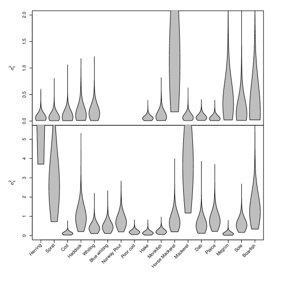
Figure 2: Violin plots showing the marginal posterior distribution for the variance parameters. The top plot shows the variance associated with the catch and the bottom shows the variance associated with the survey. Blue whiting’s variance term for the catch was large and therefore was omitted from the plot. In the top plot, we fixed $\sigma_{c}=2$ for Norway Pout and poor cod so they have been omitted from the results.

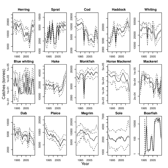
Figure 3: The median modelled commercial catches (solid black line), the 10th and 90th percentiles (dotted black lines) and the observed catches (grey line) for 15 of the 17 species. Norway pout and poor cod have been omitted as the model was not fitted to their landings. The downward spike in landings in 1999 for cod, haddock, whiting and monkfish was caused by the French not reporting landing of these stocks in that year in the dataset (ICES, 2017c).

Figure 4 shows the posterior $\phi_{1:17,1:24}$ values for each of the species except Norway pout and poor cod. It also shows the fishing mortality values from the ICES stock-assements, which use SSM, for cod, haddock, whiting, hake, megrim and herring. The cod, haddock and whiting assessments are for the Celtic Sea (ICES, 2018a, c, g), whereas the hake, megrim and herring assessments are for a larger region than our study (ICES, 2018d, e, f). With the exception of haddock, the $\phi_{1:17,1:24}$ values from this study seem to follow, at least qualitatively, that of the assessment fishing mortality.

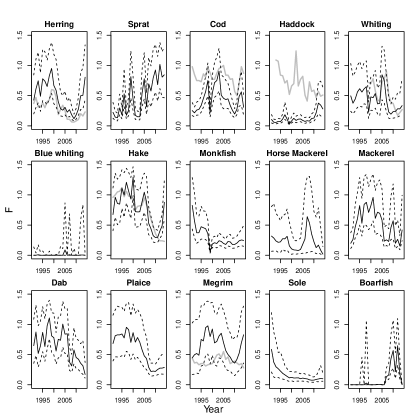
Figure 4: The median value of the fishing rates (solid black line), and the 10 and 90 percentiles, (dotted black lines) for 15 of the 17 species. Norway pout and poor cod have been omitted as the model was not fitted to their landings.

Figure 5 shows the marginal posterior distribution of the fishing rate during the spin-up period, $\phi_{i,0}$. Many of the posterior distributions are similar to their prior distributions, e.g. herring, sprat, however some of the posteriors are quite different from their priors. The fishing rates for cod and horse mackerel are low, which means that when the simulation starts in 1991, cod and horse mackerel will be in a nearly unfished state whereas hake and monkfish, which have quite high fishing rates in the spin-up period, start the simulation in an exploited state.

Figure 5: The marginal posterior distributions of the fishing rate during the spin-up period, $\phi_{0}$.

3.2 Spawning stock biomass

Figure 6 shows the median, 10th percentile and 90th percentile estimates for cod, haddock, whiting, hake, herring and megrim spawning stock biomass (SSB). It also shows the SSB estimates from ICES stock-assessments. The cod assessment and the mizer model agree towards the end of the time period. The whiting single-species and multi-species estimates are similar. Both hake assessments show an increase in SSB at about 2005 which coincides with a reduction in the fishing rate at around the same time, as shown in Figure 4; this is also visible in the stock-assessment. In addition the qualitative patterns in herring and megrim seem similar in both the MSM and the SSM. The MSM predicts different SSB for haddock than the SSM.

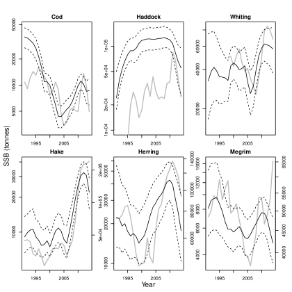
Figure 6: The median modelled SSB (solid black line), the 10 and 90 percentiles (dotted black lines) and SSB estimates from single-species ICES assessments for cod, haddock, whiting hake, megrim and herring (grey line). The hake, megrim and herring assessments cover more area than the model does and therefore is plotted on a different scale.

4 Discussion

In this study we fitted the multi-species size-based model of Blanchard et al. (2014) with 17 species in the Celtic Sea, a mechanistic model of intermediate complexity, using novel techniques to address the high dimensionality of the problem. We also demonstrated these methods in a simulation study with three species using the model of Spence et al. (2020b), also a mechanistic MSM (see Simulation study).

4.1 Mechanistic models

We found that the model was able to recreate demersal survey catches and commercial catches. The model was not able to recreate the survey data for pelagic fish. This is understandable as the IBTS survey is not so good at sampling pelagic and flatfish and therefore the noise is much greater (Walker et al., 2017). Our approach gives an idea about the magnitude of the observation uncertainty in the IBTS survey. We could further reduce uncertainty in the model by fitting to additional surveys, for example acoustic surveys.

For most of the stocks with full assessments, we get similar SSB and fishing rates, however for haddock both are qualitatively and quantitatively different. In the SSM model the recruitment rates of haddock are unpredictable (ICES, 2018c), something that is not captured by the MSM model here, which suggests that the SSB in SSMs is recruitment driven. Stochastic recruitment has been included in some MSMs (e.g. Blanchard et al., 2014; Thorpe et al., 2017), but more work is required to explore this.

Although there is such a thing as a true fishing mortality, using it as a ‘tuning parameter’, as done in this study and in many SSMs, destroys its true meaning (Rougier & Beven, 2013). For example, in the model we fitted in this study, only the fishing rates were used to drive the dynamics. Therefore, the fishing rates implicitly have information about all things that drive the dynamics of the species, e.g. environment, recruitment or migration. Although many SSMs account for dynamic recruitment (e.g. Stock Synthesis Methot & Wetzel, 2013), their fishing mortality also imply dynamics caused by interactions between different species, which is explicit in MSMs. Therefore taking fishing mortality values from other models and using them as ‘input variables’ (e.g. Thorpe et al., 2015; Spence et al., 2016; Speirs et al., 2016), can lead to systematic biases in the model (Brooks & Deroba, 2015) and so should be done with caution, however there are circumstances when it might actually be desirable. For instance it may be necessary to save on computational effort or one may want the fishing rates to represent the fishing mortality generated by stock assessments rather than the actual fishing mortality on the stock as it is possible to calculate this and manage to it (e.g. Spence et al., 2020a).

A common requirement of fisheries models is to assess the current state of a stock. SSMs and statistical MSMs, with many ‘tuning parameters’, are good at doing this when there is a lot of data. However, by fitting mechanistic MSMs directly to data, we free the model from the assessment-induced biases and could therefore contribute to the assessment processes. The natural mortality rates from mechanistic models could be used as ‘input variables’ to SSMs in regions where there is a lack of data (e.g. stomach contents data), making statistical MSMs impractical. For example, results from this Celtic Sea model could be used to generate natural mortality rates that could be used as inputs to SSMs, as currently natural mortality inputs for many of the Celtic Sea assessments come from a theoretical study (Lorenzen, 1996). For regions where statistical MSMs already exist, mechanistic MSMs could be used to corroborate or validate them, increasing our confidence in their results, to suggest an alternative or as part of an ensemble model.

Mechanistic models have been increasingly used as strategic tools when considering how populations, communities and ecosystems respond to management or environmental changes (Pikitch et al., 2004; Collie et al., 2016). They are developed with ecological and biological theory, through ‘input variables’ and processes within the model. Therefore, as this theory develops the mechanistic models become more like reality. As mechanisms and physical laws are time invariant and more robust than statistical correlations, mechanistic MSMs should enable us to make better long-term predictions as interactions between different species and different processes will be more explicit (Connor et al., 2017; Cuddington et al., 2013). This should lead to improved strategic management, for example in setting long-term targets and reference points, e.g. multi-species maximum sustainable yield. Improvements in our understanding of responses to new conditions, such as warming oceans, can readily be included in these models (e.g. Serpetti et al., 2017) and the types of actions that can be tested and implemented can be increased, e.g. spatial planning using spatially explicit mechanistic models (e.g. Ecospace Walters et al., 1999).

Before this study, fitting MSMs to species that did not have full assessments with absolute values of the fishing mortality was not possible without making strong assumptions about their fishing mortality values. This would be particularly the case for species with limited data (Quárou & Tomini, 2013). The methods of fitting dynamical parameters introduced and demonstrated here could lead to an increase in the number of mechanistic models for regions where there is not a great amount of information, hence increasing their utility and the strategic management of these areas. This could either be by sharing fishing rates between models, for example a LeMans model for the Celtic Sea could use fishing rates from this study, or directly fitting the dynamical parameters for the mechanistic model.

In addition, mechanistic models could be used to manage data-limited stocks or in areas of the world where there are many species and building a MSMs is computationally expensive or managing at the level of individual species is impracticable. The methods developed here to find dynamical parameters could be useful when fitting trait-based models, where groups of species with similar traits are grouped together (Barnett et al., 2019).

4.2 Developing the role of mechanistic models

Whilst mechanistic models are potentially powerful tools, their use to date in the advisory process has been limited. Here we suggest some improvements that should make them more useful to fisheries management.

In this work the state of the system at the beginning of the simulation, $M_{0}$, was determined by running the model for 300 years with a fixed fishing mortality $\phi_{0,1:17}$, known as the spin-up period (Spence et al., 2016). This led to the model starting in a stationary state, something which may not be true and can have an effect on the results of the model, particularly at the beginning of the simulation. For example, cod was probably not in a stationary state in 1991, as prior to the model large landings were reported in 1988-1990 (ICES, 2018a). It is not possible to create the effect of these high landings using the spin-up period, and our fitted model is therefore unable to pick up the dynamics at the beginning of the time series. The fitted model found that the spin-up fishing mortality for cod, $\phi_{0,3}$, was low (Figure 5), which lead to over-estimating the SSB (Figure 6) and the fishing mortality (Figure 4) in the early part of the simulation.

More work is required calibrating the initial state of mechanistic MSMs. In this study we initialised the model by running it model to equilibrium with a fixed fishing mortality. This meant that the system was in equilibrium at the beginning of the simulation which may not be true. One may run some dynamics, say ten years, before calibration, however it would not have been possible here as we do not know the fishing mortality rates for 1981-1991; alternatively one could run the fishing mortality time series backwards before starting to fit the data, as done in climate modelling (Stouffer et al., 2004). A common approach in other fisheries models is to treat the initial states as uncertain, i.e. treating the density for each species and the background for all sizes in mizer as uncertain parameters. We believe this would be the ideal solution, however it would lead to an impractically large number of parameters. A more practical solution may be to use ecological theory from other studies, such as fishing effects on the size-spectrum (e.g. Zhang et al., 2018), to parameterise, with only a handful of parameters, the initial state of the model. These parameters would then be calibrated to the data as well.

In this work we used the default fishing selectivity in mizer (Scott et al., 2014). Other fishing selectivity functions, such as logistic or dome shaped, may lead to different results, however we do not believe that the results would greatly change here. In the future we would like to include fisheries information, such as effort and catch by fleet or metier, and possibly by size, when fitting these models. In addition information from external studies about the selectivity of different fishing gears could be included, with the selectivity of each gear on each species being the ‘tuning parameters’ (e.g. Walker et al., 2017). One may anticipate that this may follow a dynamic stochastic process, such as an auto-regressive model, as the spatial distribution of species will not change that quickly, thus incorporating more information in the model.

With mechanistic MSMs it is not straightforward to perform conventional model validation. In the study here it was not possible to compare the model forecasts with independent out-of-sample data, e.g. the survey and commercial catches in 2015-2019, as the fishing rates, the inputs that are used to drive the dynamics that led to these data, are uncertain. Furthermore, due to the time taken to fit these models it is not practical to perform one-step-ahead analysis (Berg & Nielsen, 2016) or cross-validation tests. Instead we demonstrated through residual analysis that the conditionally independent assumptions are not violated (see Supplementary material (S4)). There are many other methods that could be used for model validation (e.g. posterior predictive checks, see Gelman et al., 2013, for more details); for a recent review of these methods see Conn et al. (2018).

4.3 Quantifying uncertainty

For models to be useful for management it is important that uncertainty is quantified (Harwood & Stokes, 2003). By fitting the model in a Bayesian framework we were able to quantify the uncertainty in the model. This is a difficult problem using conventional MCMC due to the complexity of the model, and the increased dimension of the uncertain parameters caused by fitting fishing mortality. We believe that this is a major reason why this has not previously been done. SSMs and statistical MSMs take advantage of recent software developments and are fitted using algorithms that exploit gradients, such as Hamiltonian Monte Carlo (Neal, 2010) or Reimann Manifold MCMC (Girolami & Calderhead, 2011). However, for more mechanistic-based models, this may be impractical or even impossible. In this paper we have demonstrated a method of exploiting the stucture of the model to use an MCMC algorithm to fit a mechanistic model.

For mechanistic-based models, where the model needs to be run to evaluate the likelihood, it is advantageous to use parallel computing, running several likelihood evaluations at once, to speed up the fitting process. The problem here is that MCMC is a sequential algorithm and therefore difficult to run in parallel (Jacob et al., 2011). In this paper we introduce two novel variations of the delayed-acceptance MCMC algorithm (Sherlock et al., 2017). The MDA-MCMC algorithm is designed to use parallel computing and is motivated by attempting to move many parameters at once, accepting the good moves whilst rejecting the bad ones. We believe that the MDA-MCMC would be most useful when sets of parameters, or transformations of the parameters, affect different parts of the likelihood. This could be explored using variance-based sensitivity analysis (Saltelli et al., 2008) prior to running the algorithm. As the MDA-MCMC algorithm makes moves in smaller dimensions, the proposals can be larger in the parameter space. We recommend the proposals are large so that the resulting in acceptance probabilities, in the first part of the algorithm, are either 0 or 1. This would mean that the accepted points result in large improvements in the full likelihood.

Similarly the PDA-MCMC is motivated by proposing moves in a large number of dynamical parameters but efficiently accepting only the good moves. If one was going to fit the dynamical parameters by hand, one might wish to change the fishing rates one year at a time and to run that model for one year. The PDA-MCMC algorithm does just that but in such a way that the stationary distribution of the Markov chain is the posterior distribution. An alternative would be to change one year at each iteration of the MCMC chain, therefore requiring 24 model runs all of which are required to be done sequentially, whereas using the PDA-MCMC algorithm it only requires five model runs, most of which can be run in parallel. This therefore leads to more efficient use of computational effort when updating dynamical parameters such as annual fishing rates. The PDA-MCMC algorithm can also be flexible when deciding which of the dynamical parameters are changed. In the study in the manuscript we attempted to change all of the dynamical parameters at once, however in the Simulation study we only changed a handful of dynamical parameters at a time, something that we found led to better mixing. The PDA-MCMC algorithm is also useful when the state of the model is dependent on the entire past and/or is stochastic. To do this one would require $M_{t}$ to include the whole of the past. If the model was stochastic, we recommend treating the stochastic elements as additional parameters, as in Spence & Blackwell (2016) allowing better exploration of the dynamical parameter space. These two algorithms are not specific to MSMs, or even mechanistic models, but are applicable to a wide range of MCMC problems.

4.4 Conclusion

We have demonstrated a method of fitting mechanistic MSMs directly to data without using SSMs. By using novel techniques we were able to fit a model of intermediate complexity in a high-dimensional parameter space with quantifiable uncertainty. Furthermore, by fitting mechanistic MSMs directly to data, we free the model from the assessment-induced biases, which may lead to a greater reliability and trust in mechanistic models, increasing their utility in the management process.

Although demonstrated on two multi-species marine models, this methodology is readily generalisable for fitting models of intermediate complexity (with a typical run time of 1 second to a few minutes), when there are a significant number of uncertain dynamic parameters. It is therefore likely to find wide applications throughout science.

Authors’ contribution

MAS conceived the ideas and designed the methodology; MAS, RTB, and PGB fit the model to the data; RS, FS and JLB developed the model used in the case study; MAS led the writing of the manuscript. All authors contributed critically to the drafts and gave final approval for publication

Data availability statement

Data sharing is not applicable to this article as no new data were created; rather, data were acquired from existing published sources (all sources are cited in the text), or are described, figured and tabulated within the manuscript or supplementary information of this article.

References

- Aeberhard et al. (2018) Aeberhard, W.H., Mills Flemming, J. & Nielsen, A. (2018) Review of State-Space Models for Fisheries Science. Annual Review of Statistics and Its Application, 5, 215–235.
- Anon (2015) Anon (2015) Celtic sea case study. Case study presentation and summary of biological knowledge, pp. 76–91. https://www.discardless.eu/media/results/Celtic_Sea_case_study.pdf.
- Barnett et al. (2019) Barnett, L.A.K., Jacobsen, N.S., Thorson, J.T. & Cope, J.M. (2019) Realizing the potential of trait-based approaches to advance fisheries science. Fish and Fisheries, 20, 1034–1050.
- Bayes (1763) Bayes, T. (1763) LII. An essay towards solving a problem in the doctrine of chances. By the late Rev. Mr. Bayes, F. R. S. communicated by Mr. Price, in a letter to John Canton, A. M. F. R. S. Philosophical Transactions, 53, 370–418.
- Berg & Nielsen (2016) Berg, C.W. & Nielsen, A. (2016) Accounting for correlated observations in an age-based state-space stock assessment model. ICES Journal of Marine Science, 73, 1788–1797.
- Blanchard et al. (2014) Blanchard, J.L., Andersen, K.H., Scott, F., Hintzen, N.T., Piet, G. & Jennings, S. (2014) Evaluating targets and trade-offs among fisheries and conservation objectives using a multispecies size spectrum model. Journal of Applied Ecology, 51, 612–622.
- Brooks & Deroba (2015) Brooks, E.N. & Deroba, J.J. (2015) When “data” are not data: the pitfalls of post hoc analyses that use stock assessment model output. Canadian Journal of Fisheries and Aquatic Sciences, 72, 634–641.
- Brynjarsdóttir & O’Hagan (2014) Brynjarsdóttir, J. & O’Hagan, A. (2014) Learning about physical parameters: the importance of model discrepancy. Inverse Problems, 30, 114007.
- Calderhead (2014) Calderhead, B. (2014) A general construction for parallelizing Metropolis-Hastings algorithms. Proceedings of the National Academy of Sciences, 111, 17408–17413.
- Collie et al. (2016) Collie, J.S., Botsford, L.W., Hastings, A., Kaplan, I.C., Largier, J.L., Livingston, P.A., Plagànyi, E., Rose, K.A., Wells, B.K. & Werner, F.E. (2016) Ecosystem models for fisheries management: finding the sweet spot. Fish and Fisheries, 17, 101–125.
- Conn et al. (2018) Conn, P.B., Johnson, D.S., Williams, P.J., Melin, S.R. & Hooten, M.B. (2018) A guide to bayesian model checking for ecologists. Ecological Monographs, 88, 526–542.
- Connor et al. (2017) Connor, L., Matson, R. & Kelly, F.L. (2017) Length-weight relationships for common freshwater fish species in Irish lakes and rivers. Biology and Environment: Proceedings of the Royal Irish Academy, 117B, 65–75.
- Cuddington et al. (2013) Cuddington, K., Fortin, M.J., Gerber, L.R., Hastings, A., Liebhold, A., O’Connor, M. & Ray, C. (2013) Process-based models are required to manage ecological systems in a changing world. Ecosphere, 4, art20.
- Cui et al. (2011) Cui, T., Fox, C., Nicholls, G. & O’Sullivan, M. (2011) Using Parallel MCMC Sampling to Calibrate a Computer Model of a Geothermal reservoir. Technical report, Report University of Auckland Faculty of Engineering 686.
- Evensen (2003) Evensen, G. (2003) The ensemble kalman filter: theoretical formulation and practical implementation. Ocean Dynamics, 53, 343–367.
- FAO (2009) FAO (2009) How to Feed the World in 2050 - Food and Agriculture organization. Http://www.fao.org/docrep/pdf/012/ak542e/ak542e00.pdf.
- Farcas & Rossberg (2016) Farcas, A. & Rossberg, A.G. (2016) Maximum sustainable yield from interacting fish stocks in an uncertain world: two policy choices and underlying trade-offs. ICES Journal of Marine Science, 73, 2499–2508.
- Farnsworth et al. (2014) Farnsworth, K.D., Shephard, S., Reid, D.G. & Gerritsen, H.D. (2014) Estimating biomass, fishing mortality, and “total allowable discards” for surveyed non-target fish. ICES Journal of Marine Science, 72, 458–466.
- Fasiolo et al. (2016) Fasiolo, M., Pya, N. & Wood, S.N. (2016) A Comparison of Inferential Methods for Highly Nonlinear State Space Models in Ecology and Epidemiology. Statist Sci, 31, 96–118.
- Fournier et al. (2012) Fournier, D.A., Skaug, H.J., Ancheta, J., Ianelli, J., Magnusson, A., Maunder, M.N., Nielsen, A. & Sibert, J. (2012) AD Model Builder: using automatic differentiation for statistical inference of highly parameterized complex nonlinear models. Optimization Methods and Software, 27, 233–249.
- Frid & Paramor (2012) Frid, C.L.J. & Paramor, O.A.L. (2012) Feeding the world: what role for fisheries? ICES Journal of Marine Science, 69, 145–150.
- Gelman et al. (2013) Gelman, A., Carlin, J., Stern, H., Dunson, D., Vehtari, A. & Rubin, D. (2013) Bayesian Data Analysis. Chapman and Hall/CRC, third edition edition.
- Girolami & Calderhead (2011) Girolami, M. & Calderhead, B. (2011) Riemann manifold Langevin and Hamiltonian Monte Carlo methods. Journal of the Royal Statistical Society: Series B (Statistical Methodology), 73, 123–214.
- Gordon et al. (1993) Gordon, N.J., Salmond, D.J. & Smith, A.F.M. (1993) Novel approach to nonlinear/non-gaussian bayesian state estimation. IEE Proceedings F - Radar and Signal Processing, 140, 107–113.
- Hartvig et al. (2011) Hartvig, M., Andersen, K.H. & Beyer, J.E. (2011) Food web framework for size-structured populations. Journal of Theoretical Biology, 272, 113 – 122.
- Harwood & Stokes (2003) Harwood, J. & Stokes, K. (2003) Coping with uncertainty in ecological advice: lessons from fisheries. Trends in Ecology & Evolution, 18, 617 – 622.
- Hastings (1970) Hastings, W.K. (1970) Monte carlo sampling methods using markov chains and their applications. Biometrika, 57, 97–109.
- Hatton et al. (2015) Hatton, I.A., McCann, K.S., Fryxell, J.M., Davies, T.J., Smerlak, M., Sinclair, A.R.E. & Loreau, M. (2015) The predator-prey power law: Biomass scaling across terrestrial and aquatic biomes. Science, 349.
- Heath (2012) Heath, M.R. (2012) Ecosystem limits to food web fluxes and fisheries yields in the North sea simulated with an end-to-end food web model. Progress in Oceanography, 102, 42 – 66. End-to-End Modeling: Toward Comparative Analysis of Marine Ecosystem Organization.
- Heymans et al. (2016) Heymans, J.J., Coll, M., Link, J.S., Mackinson, S., Steenbeek, J., Walters, C. & Christensen, V. (2016) Best practice in ecopath with ecosim food-web models for ecosystem-based management. Ecological Modelling, 331, 173 – 184. Ecopath 30 years – Modelling ecosystem dynamics: beyond boundaries with EwE.
- ICES (2017a) ICES (2017a) 01 WGSAM - Report of the Working Group on Multispecies Assessment Methods. Technical report, International Council for Exploration of the Seas.
- ICES (2017b) ICES (2017b) Database of Trawl Surveys (DATRAS). http://datras.ices.dk.
- ICES (2017c) ICES (2017c) Official Nominal Catches. http://ices.dk/marine-data/dataset-collections/Pages/Fish-catch-and-stock-assessment.aspx.
- ICES (2018a) ICES (2018a) Cod (Gadus morhua) in divisions 7.e–k (western English Channel and southern Celtic Seas) . Technical report, International Council for Exploration of the Seas.
- ICES (2018b) ICES (2018b) Cod (Gadus morhua) in Subarea 4, Division 7.d, and Subdivision 20 (North Sea, eastern English Channel, Skagerrak). Technical report, International Council for Exploration of the Seas.
- ICES (2018c) ICES (2018c) Haddock (Melanogrammus aeglefinus) in Divisions 7.b–k (southern Celtic Seas and English Channel) . Technical report, International Council for Exploration of the Seas.
- ICES (2018d) ICES (2018d) Hake (Merluccius merluccius) in subareas 4, 6, and 7, and divisions 3.a, 8.a–b, and 8.d, Northern stock (Greater North Sea, Celtic Seas, and the northern Bay of Biscay). Technical report, International Council for Exploration of the Seas.
- ICES (2018e) ICES (2018e) Herring (Clupea harengus) in divisions 7.a South of 5230?N, 7.g-h, and 7.j-k (Irish Sea, Celtic Sea, and southwest of Ireland). Technical report, International Council for Exploration of the Seas.
- ICES (2018f) ICES (2018f) Megrim (Lepidorhombus whiffiagonis) in divisions 7.b-k, 8.a-b, and 8.d (west and southwest of Ireland, Bay of Biscay) . Technical report, International Council for Exploration of the Seas.
- ICES (2018g) ICES (2018g) Whiting (Merlangius merlangus) in divisions 7.b-c and 7.e–k (southern Celtic Seas and eastern English Channel). Technical report, International Council for Exploration of the Seas.
- Jacob et al. (2011) Jacob, P., Robert, C.P. & Smith, M.H. (2011) Using Parallel Computation to Improve Independent Metropolis-Hastings Based Estimation. Journal of Computational and Graphical Statistics, 20, 616–635.
- Jonsen et al. (2005) Jonsen, I.D., Flemming, J.M. & Myers, R.A. (2005) Robust state-space modeling of animal movement data. Ecology, 86, 2874–2880.
- Lewy & Vinther (2004) Lewy, P. & Vinther, M. (2004) A stochastic age-length-structured multispecies model applied to north sea stocks. Technical report, ICES.
- Link et al. (2011) Link, J.S., Bundy, A., Overholtz, W.J., Shackell, N., Manderson, J., Duplisea, D., Hare, J., Koen-Alonso, M. & Friedland, K.D. (2011) Ecosystem-based fisheries management in the Northwest Atlantic. Fish and Fisheries, 12, 152–170.
- Liu & Chen (1998) Liu, J.S. & Chen, R. (1998) Sequential monte carlo methods for dynamic systems. Journal of the American Statistical Association, 93, 1032–1044.
- Lorenzen (1996) Lorenzen, K. (1996) The relationship between body weight and natural mortality in juvenile and adult fish: a comparison of natural ecosystems and aquaculture. Journal of Fish Biology, 49, 627–642.
- Mackinson et al. (2018) Mackinson, S., Platts, M., Garcia, C. & Lynam, C. (2018) Evaluating the fishery and ecological consequences of the proposed North Sea multi-annual plan. PLOS ONE, 13, 1–23.
- Methot & Wetzel (2013) Methot, R.D. & Wetzel, C.R. (2013) Stock synthesis: A biological and statistical framework for fish stock assessment and fishery management. Fisheries Research, 142, 86 – 99.
- Metropolis et al. (1953) Metropolis, N., Rosenbluth, A.W., Rosenbluth, M.N., Teller, A.H. & Teller, E. (1953) Equation of state calculations by fast computing machines. The Journal of Chemical Physics, 21, 1087–1092.
- Neal & Roberts (2006) Neal, P. & Roberts, G. (2006) Optimal scaling for partially updating MCMC algorithms. Ann Appl Probab, 16, 475–515.
- Neal (2010) Neal, R.M. (2010) Handbook of Markov Chain Monte Carlo, chapter MCMC Using Hamiltonian Dynamics, pp. 113–162. Chapman & Hall/CRC.
- Nielsen & Berg (2014) Nielsen, A. & Berg, C.W. (2014) Estimation of time-varying selectivity in stock assessments using state-space models. Fisheries Research, 158, 96 – 101. SI: Selectivity.
- Pikitch et al. (2004) Pikitch, E.K., Santora, C., Babcock, E.A., Bakun, A., Bonfil, R., Conover, D.O., Dayton, P., Doukakis, P., Fluharty, D., Heneman, B., Houde, E.D., Link, J., Livingston, P.A., Mangel, M., McAllister, M.K., Pope, J. & Sainsbury, K.J. (2004) Ecosystem-Based Fishery Management. Science, 305, 346–347.
- Plagányi et al. (2014) Plagányi, E.E., Punt, A.E., Hillary, R., Morello, E.B., Thébaud, O., Hutton, T., Pillans, R.D., Thorson, J.T., Fulton, E.A., Smith, A.D.M., Smith, F., Bayliss, P., Haywood, M., Lyne, V. & Rothlisberg, P.C. (2014) Multispecies fisheries management and conservation: tactical applications using models of intermediate complexity. Fish and Fisheries, 15, 1–22.
- Quárou & Tomini (2013) Quárou, N. & Tomini, A. (2013) Managing interacting species in unassessed fisheries. Ecological Economics, 93, 192 – 201.
- Railsback & Grimm (2011) Railsback, S.F. & Grimm, V. (2011) Agent-Based and Individual-Based Modeling A practical Introduction. Princeton University Press, first edition edition.
- Rougier & Beven (2013) Rougier, J.C. & Beven, K.J. (2013) Model and data limitations: the sources and implications of epistemic uncertainty, pp. 40–63. Cambridge University Press.
- Saltelli et al. (2008) Saltelli, A., Ratto, M., Andres, T., Campolongo, F., Cariboni, J., Gatelli, D., Salsana, M. & Tarantola, S. (2008) Global sensitivity analysis - The primer. Wiley.
- Scott et al. (2014) Scott, F., Blanchard, J.L. & Andersen, K.H. (2014) mizer: an R package for multispecies, trait-based and community size spectrum ecological modelling. Methods in Ecology and Evolution, 5, 1121–1125.
- Serpetti et al. (2017) Serpetti, N., Baudron, A.R., Burrows, M.T., Payne, B.L., Helaouët, P., Fernandes, P.G. & Heymans, J.J. (2017) Impact of ocean warming on sustainable fisheries management informs the ecosystem approach to fisheries. Scientific Reports, 7, 13438.
- Sherlock et al. (2017) Sherlock, C., Golightly, A. & Henderson, D.A. (2017) Adaptive, Delayed-Acceptance MCMC for Targets With Expensive Likelihoods. Journal of Computational and Graphical Statistics, 26, 434–444.
- Skaug & Fournier (2006) Skaug, H.J. & Fournier, D.A. (2006) Automatic approximation of the marginal likelihood in non-gaussian hierarchical models. Computational Statistics & Data Analysis, 51, 699 – 709.
- Speirs et al. (2016) Speirs, D., Greenstreet, S. & Heath, M. (2016) Modelling the effects of fishing on the North Sea fish community size composition. Ecological Modelling, 321, 35–45.
- Spence et al. (2020a) Spence, M.A., Alliji, K., Bannister, H.J., Walker, N.D. & Muench, A. (2020a) Fish should not be in isolation: Calculating maximum sustainable yield using an ensemble model.
- Spence et al. (2020b) Spence, M.A., Bannister, H.J., Ball, J.E., Dolder, P.J., Griffiths, C.A. & Thorpe, R.B. (2020b) LeMaRns: A Length-based Multi-species analysis by numerical simulation in R. PLOS ONE, 15, 1–12.
- Spence & Blackwell (2016) Spence, M.A. & Blackwell, P.G. (2016) Coupling random inputs for parameter estimation in complex models. Statistics and Computing, 26, 1137–1146.
- Spence et al. (2016) Spence, M.A., Blackwell, P.G. & Blanchard, J.L. (2016) Parameter uncertainty of a dynamic multispecies size spectrum model. Canadian Journal of Fisheries and Aquatic Sciences, 73, 589–597.
- Spence et al. (2018) Spence, M.A., Blanchard, J.L., Rossberg, A.G., Heath, M.R., Heymans, J.J., Mackinson, S., Serpetti, N., Speirs, D.C., Thorpe, R.B. & Blackwell, P.G. (2018) A general framework for combining ecosystem models. Fish and Fisheries, 19, 1031–1042.
- Stouffer et al. (2004) Stouffer, R.J., Weaver, A.J. & Eby, M. (2004) A method for obtaining pre-twentieth century initial conditions for use in climate change studies. Climate Dynamics, 23, 327–339.
- Thorpe et al. (2017) Thorpe, R.B., Jennings, S., Dolder, P.J. & editor: Shijie Zhou, H. (2017) Risks and benefits of catching pretty good yield in multispecies mixed fisheries. ICES Journal of Marine Science, 74, 2097–2106.
- Thorpe et al. (2015) Thorpe, R.B., Le Quesne, W.J.F., Luxford, F., Collie, J.S. & Jennings, S. (2015) Evaluation and management implications of uncertainty in a multispecies size-structured model of population and community responses to fishing. Methods in Ecology and Evolution, 6, 49–58.
- Tierney & Kadane (1986) Tierney, L. & Kadane, J.B. (1986) Accurate approximations for posterior moments and marginal densities. Journal of the American Statistical Association, 81, 82–86.
- Tyrrell et al. (2011) Tyrrell, M., Link, J. & Moustahfid, H. (2011) The importance of including predation in fish population models: Implications for biological reference points. Fisheries Research, 108, 1 – 8.
- Vernon et al. (2014) Vernon, I., Goldstein, M. & Bower, R. (2014) Galaxy formation : Bayesian history matching for the observable universe. Statistical science, 29, 81–90.
- Walker et al. (2017) Walker, N.D., Maxwell, D.L., Le Quesne, W.J.F. & Jennings, S. (2017) Estimating efficiency of survey and commercial trawl gears from comparisons of catch-ratios. ICES Journal of Marine Science, 74, 1448–1457.
- Walters et al. (1999) Walters, C., Pauly, D. & Christensen, V. (1999) Ecospace: Prediction of mesoscale spatial patterns in trophic relationships of exploited ecosystems, with emphasis on the impacts of marine protected areas. Ecosystems, 2, 539–554.
- Wan & Van Der Merwe (2000) Wan, E.A. & Van Der Merwe, R. (2000) The unscented Kalman filter for nonlinear estimation. Proceedings of the IEEE 2000 Adaptive Systems for Signal Processing, Communications, and Control Symposium (Cat. No.00EX373), pp. 153–158.
- White & Marshall (2019) White, C.R. & Marshall, D.J. (2019) Should We Care If Models Are Phenomenological or Mechanistic? Trends in Ecology & Evolution, 34, 276– 278.
- Zhang et al. (2018) Zhang, C., Chen, Y., Xu, B., Xue, Y. & Ren, Y. (2018) Evaluating fishing effects on the stability of fish communities using a size-spectrum model. Fisheries Research, 197, 123 – 130.
- Zucchini et al. (2016) Zucchini, W., MacDonald, I.L. & Langrock, R. (2016) HiddenMarkov Models for Time Series: An Introduction Using R, Second Edition. Chapman & Hall/CRC Monographs on Statistics & Applied Probability.