Nonlinear dynamics of superpostion of wavepackets

Abstract

We study nonlinear dynamics of superposition of quantum wavepackets in various systems such as Kerr medium, Morse oscillator and bosonic Josephson junction. The prime reason behind this study is to find out how the superposition of states influence the dynamics of quantum systems. We consider the superposition states which are potential candidates for quantum computing and quantum communication and so it is most necessary that we study the dynamics for their proper understanding and usage. Methods in nonlinear time series analysis such as first return time distribution, recurrence plot and Lyapunov exponent are used for the qualification and quantification of dynamics. We found that there is a vast change in the dynamics of quantum systems when we consider the superposition of wave packets. These changes are observed in various kinds of dynamics such as periodic, quasi-periodic, ergodic, and chaotic dynamics.

I Introduction

Quantum superposition is one of the most fundamental features of quantum mechanics Dirac (1981) with which one can explain the quantum effects arising from the interference of quantum amplitudes. In classical physics, it is possible to have a superposition of fields which will give rise to a new field  but  the quantum mechanical concept  of probability to occur the individual states is not feasible da Costa and De Ronde (2013). The properties of these quantum superposition states can be used in various applications of quantum information theory such as quantum communication, quantum teleportation, quantum cryptography, quantum cloning Feix et al. (2015); Bennett et al. (1992); Milburn and Braunstein (1999); Ralph et al. (2003); Cerf et al. (2000) etc. It is a well-established fact that various non-classical effects such as squeezing, higher-order squeezing, sub-Poissonian statistics and oscillations of the photon number distribution are exhibited by superposition of coherent states Bužek et al. (1992); Gerry (1993) in contrast to ordinary coherent states. Various theoretical Yurke and Stoler (1986); Miranowicz et al. (1990); Paprzycka and Tanas (1992); Tara et al. (1993) and experimental methods Monroe et al. (1996); Ourjoumtsev et al. (2007); Gao et al. (2010) are also available for the production of superposition states. The experimental observation of Schrödinger cat states, which is a superposition state, using the single-photon Kerr effect has opened new directions in continuous variable quantum communication Kirchmair (2013).

On the other hand, extensive studies have been carried out on the dynamics of quantum systems but less has been done for the dynamics of superposition states. Ergodicity in quantum systems has received much attention after the quantum ergodic theory proposed by von Neumann in as early 1929 Von Neumann (1929). Later, Peres gave the newest definition of quantum ergodicity as the time average of any quantum operator equal to its average of microcanonical ensemble Peres (1984). If the motion evolves to exponentially separated trajectories even for nearly identical initial conditions, such types are referred to as chaotic. Chaos is a type of motion that lies between the regular deterministic trajectories arising from solutions of integrable equations and a state of noise or stochastic behaviour characterized by complete randomness Goldstein et al. (2014). Nonlinear dynamics of quantum systems have been of special interest and have been studied by many Scott and Milburn (2001); Maletinsky et al. (2007); Bettelheim et al. (2007); Wang et al. (2014). Various methods are available to study the nonlinear dynamics of quantum systems such as random matrix theory Mehta (2004); Andreev et al. (1996), recurrence time distributions and recurrence quantification analysis Eckmann et al. (1987); Marwan et al. (2007) and Lyapunov spectra Rosenstein et al. (1993); Kantz (1994). In the literature, expectation values of certain dynamical variables are considered as time series to study quantum dynamics of various systems Sudheesh et al. (2009, 2010); Shankar et al. (2014); Pradeep et al. (2020). There are a few studies addressing the dynamics of superposition of wave packets, for example, fractional revivals of superposed wave packets in a nonlinear Hamiltonian Rohith and Sudheesh (2014, 2015). However, qualitatively different, such as quasi-periodic, ergodic, and chaotic behavior in the dynamics of a superposition of quantum wave packets are not reported. In this review paper, we would like to study in detail the dynamics of superposition of quantum wavepackets and investigate how the superposition alter the dynamics of quantum systems. We use time series generated from expectation values for studying the dynamics of superposition states to show the differences between superposition states and non-superposition states in terms of periodic, ergodic and chaotic dynamics.

This paper is organized as follows. In Sec. II, we study and analyze the periodic properties of expectation values of initial superposition states for two different quantum systems which are governed by nonlinear Hamiltonians. In Sec. III, we find the first return time distribution, recurrence plot and Lyapunov exponent using time series data of expectation values for different quantum states and its superposition states. The chaotic and ergodic properties of the systems are analyzed in this section. In Sec. IV, we summarize the main results of the paper.

II Periodicity of expectation values

The dynamics of a normalized quantum system $\left|{\psi(0)}\right\rangle$ is said to be periodic if the autocorrelation function $\left|{\langle{\psi(t)}|{\psi(0)}\rangle}\right|^{2}$ becomes unity, where $\left|{\psi(t)}\right\rangle$ is the time evolved state. When a quantum system is periodic, all expectation values of the system attains its initial value periodically. Various quantum systems showing periodic dynamics can be seen in the literature Robinett (2004). Harmonic oscillator, infinite well etc., are popular systems showing periodic dynamics. We will be studying similar periodicity in the time evolution of quantum systems governed by nonlinear Hamiltonians. In this section, we show how the period of expectation values of certain quantum variables changes with respect to the initial states which are superposition of quantum states. For this purpose, we consider the dynamics of superposition states in Kerr medium and Morse oscillator.

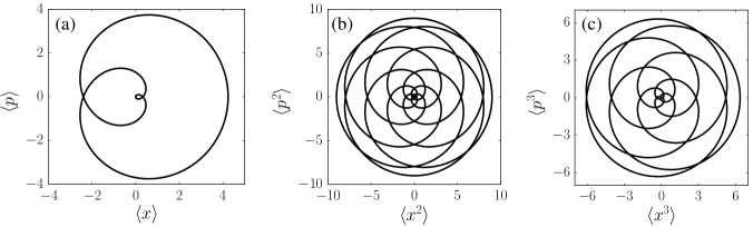
Figure 1: Plots showing the revival of (a) coherent state ($l=1$) and its superposition states with (b) $l=2$ and (c) ($l=3$). The expectation values are plotted from $t=0$ to (a) $t=\frac{\pi}{\chi}$, (b) $\frac{\pi}{\chi}$ and (c) $\frac{\pi}{3\chi}$. These closed curves indicates that these states are having periodic dynamics with different time period.

II.1 Dynamics of superposition states in a Kerr medium

Consider the dynamics governed by a nonlinear Hamiltonian which is the effective Hamiltonian for the propagation of coherent field in a Kerr medium Milburn (1986); Kitagawa and Yamamoto (1986)

$$H=\hslash\chi{\hat{a}^{{\dagger}2}}\hat{a}^{2}=\hslash\chi{N}({N}-1),$$ (1)

where $\hat{a}$ and $\hat{a}^{{\dagger}}$ are annihilation and creation operators. The operator ${N}={a}^{{\dagger}}{a}$ is the number operator whose eigenstates are the Fock state $\left|{n}\right\rangle$, where $n=0,\,1,\,2\,\dots\infty$ and $\chi$ is the nonlinear susceptibility of the medium. Consider a general wavepacket $\left|{\psi(0)}\right\rangle$ which can be expanded in the Fock basis as

$$\left|{\psi(0)}\right\rangle=\sum_{n=0}^{\infty}C_{n}\left|{n}\right\rangle,$$ (2)

where $C_{n}$ are the Fock state expansion coefficients. Using the unitary time evolution opetator $e^{-iHt/\hslash}$, we can obtain the state at time $t$:

$$\left|{\psi(t)}\right\rangle=e^{-iHt/\hslash}\left|{\psi(0)}\right\rangle.$$ (3)

Let a coherent state $\left|{\alpha(0)}\right\rangle$ be the initial wave packet which is the eigenstate of the annihilation operator $\hat{a}$ with eigenvalue $\alpha$. The state at time $t$ can be expressed in the Fock basis as

$$\left|{\alpha(t)}\right\rangle=e^{-{\left|{\alpha}\right|^{2}}/{2}}\sum_{n=0}^{\infty}e^{-i\chi n(n-1)t}\frac{\alpha^{n}}{\sqrt{n!}}\left|{n}\right\rangle.$$ (4)

At time $t=\pi/\chi$ and its integer multiple instants, the system becomes periodic. In other words, at these instants the fidelity $\left|{\langle{\alpha(t)}|{\alpha(0)}\rangle}\right|^{2}$ becomes unity. This result was already appeared in Tara et al. (1993). From now on, we use $T_{per}$ to denote the time period of systems which are having periodicity. Our interest is to find how the time period $T_{per}=\pi/\chi$ changes when we consider initial states which are superpositions of coherent states. For this purpose, we consider a general superposition of $\ell$ coherent states Napoli and Messina (1999)

$$\left|{\Psi_{\ell}(0)}\right\rangle=N_{\ell}\sum_{j=0}^{\ell-1}\left|{\alpha\varepsilon_{j}^{(\ell)}}\right\rangle.$$ (5)

where $N_{\ell}$ is the normalization constant and

$$\varepsilon_{j}^{(\ell)}\equiv e^{i{2\pi}j/{\ell}}.$$ (6)

The superposition state $\left|{\Psi_{\ell}(0)}\right\rangle$ can be expanded in the Fock basis as

$$\left|{\Psi_{\ell}(0)}\right\rangle=N_{\ell}\sum_{n=0}^{\infty}\frac{\alpha^{\ell n}}{\sqrt{(\ell n)!}}\ell\left|{\ell n}\right\rangle.$$ (7)

To derive the above expression, we have used the well-known identity

$$\sum_{j=0}^{\ell-1}(\varepsilon_{j}^{(\ell)})^{n}=\ell\delta_{[\frac{n}{\ell}],\frac{n}{l}},$$ (8)

where $\delta$ is the Kronecker delta and $[\,\,\,]$ denotes the greatest integer function. The state at any time $t$, using the Kerr Hamiltonian given in Eq. (1), is

$$\left|{\Psi_{l}(t)}\right\rangle=\textit{N}_{l}\sum_{n=0}^{\infty}e^{-i\chi\ell n(\ell n-1)t}\frac{\alpha^{\ell n}}{\sqrt{\ell n!}}\ell\left|{\ell n}\right\rangle.$$ (9)

The above equation is for a general superposition of $\ell$ coherent states. Now we specifically look at the case $\ell=2$. With $l=2$ in Eq. (5), we get a superposition of two coherent states $\left|{\alpha}\right\rangle$ and $\left|{-\alpha}\right\rangle$ which is known as the even coherent state Dodonov et al. (1974).

The time evolution of an initial even coherent state gives

$$\left|{\Psi_{2}(t)}\right\rangle=N_{2}\sum_{n=0}^{\infty}e^{-i\chi 2n(2n-1)t}\frac{\alpha^{2n}}{\sqrt{2n!}}2\left|{2n}\right\rangle.$$ (10)

It is evident that this state also has the same periodicity of $\pi/\chi$ obtained for initial coherent state.

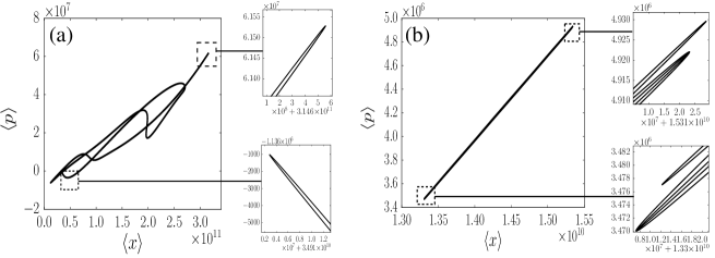
Figure 2: Plots showing the periodic dynamics of (a) coherent state ($l=1$) and (b) its superposition state ($l=2$). The expectation values are plotted from $t=0$ to (a) $t=T_{per}$, and (b) $T_{per}/4$. The closed curves indicates that the variables $\left\langle{x}\right\rangle$ and $\left\langle{p}\right\rangle$ return to its initial values at these instances.

However, when we increase the value of $\ell$, the periodicity depends on the value of $\ell$. The following results can be obtained from Eq. (11): If $\ell$ is an even number then $T_{per}={2\pi}/{\chi\ell}$. If it is odd then $T_{per}={\pi}/{\chi\ell}$.

Figure 1 shows the above results for certain values of $\ell$ using the expectation values and higher moments of the dynamical quantities $x$ and $p$ where

$$x = \dfrac{\hat{a}+\hat{a}^{\dagger}}{\sqrt{2}}\qquad\text{and}$$ (11)

$$p = \dfrac{\hat{a}-\hat{a}^{\dagger}}{i\sqrt{2}}.$$ (12)

Figure 1(a) shows the plot of $\langle x\rangle$ versus $\langle p\rangle$ for the case $\ell=1$. Figure 1(b) is plotted between $\langle x^{2}\rangle$ and $\langle p^{2}\rangle$ for the case $\ell=2$ state and Fig. 1(c) is between $\langle x^{3}\rangle$ and $\langle p^{3}\rangle$ for $\ell=3$. The closed curve in all the plots is an indicator of periodic dynamics for corresponding quantum states. We have shown that periodicity of the motion changes when we change the initial state to a superposition state. In the next session, we consider the dynamics of Morse oscillator system which also illustrate similar results.

II.2 Periodic dynamics of Morse oscillator

The Morse oscillator is a model for a particle in a one-dimensional anharmonic potential energy surface with a dissociative limit at infinite displacementMorse (1929). The Morse potential describing the vibrational motion of a diatomic molecule can be expressed as

$$V(x)=D(e^{-2\beta x}-2e^{-\beta x}),$$ (13)

where $D$ is the dissociation energy, $\beta$ is a range parameter and $x$ gives the relative distance from the equilibrium position. The eigenfunctions of the Morse potential for the reduced one body system can be written as

$$\Psi_{n}^{\lambda}(\xi)=\text{N}e^{-\xi/2}\xi^{s/2}L_{n}^{s}(\xi),$$ (14)

where $\xi=2\lambda$$e^{-\beta x}$, $0<\xi<\infty$ and $n=0,1,\dots,[\lambda-1/2]$, with $[\text{ }]$ being the greatest integer function. Here $\lambda$ and $s$ are the potential and energy dependent parameters:

$$\lambda=\sqrt{\frac{2\mu Dr_{0}^{2}}{\beta^{2}\hslash^{2}}},\text{ }s=\sqrt{\frac{-8\mu r_{0}^{2}E}{\beta^{2}\hslash^{2}}}$$ (15)

where $\mu$ is the reduced mass of the system and $r_{0}$ is the equilibrium position. In Eq. (14) $L_{n}^{s}$ is the associated Laguerre polynomial and N the normalization constant given by

$$\text{N}=\left[\dfrac{\beta(2\lambda-2n-1)\Gamma(n+1)}{\Gamma(2\lambda-n)r_{0}}\right]^{1/2}.$$ (16)

Using the annihilation and creation operators for the Morse Hamiltonian Dong et al. (2002), a displacement operator is defined Ghosh et al. (2006) which acts on the highest bound state $(\Psi_{n^{\prime}}^{\lambda}(\xi))$ to produce a Perelomov coherent state. The general expression for the coherent state is given as

$$\chi(\xi)=\sum_{n=0}^{n^{\prime}}d_{n}\Psi_{n}^{\lambda}(\xi).$$ (17)

where ${n^{\prime}}$ corresponds to the highest bound state and

$$d_{n}=\frac{(-\alpha)^{n^{\prime}-n}}{(n^{\prime}-n)!}\sqrt{\frac{n^{\prime}!\Gamma(2\lambda-n)}{n!\Gamma(2\lambda-n^{\prime})}}.$$ (18)

The distribution of $d_{n}$ or the value of $\alpha$ decides the localization of the coherent state. To study the dynamics under Morse potential, let us look at the time evolution of this wave function

$$\chi(\xi,t)=\sum_{n=0}^{n^{\prime}}d_{n}\Psi_{n}^{\lambda}(\xi)e^{{-iE_{n}t}/{\hslash}}.$$ (19)

For the Morse oscillator Strekalov (2016),

$$E_{n}=E_{0}+\hslash(\omega n-x_{e}\omega_{e}n^{2})$$ (20)

where the harmonic frequency is given by

$$\omega_{e}=\dfrac{\hslash\beta^{2}}{\mu}\left(N_{n}+\dfrac{1}{2}\right)=\sqrt{\frac{2D\beta^{2}}{\mu}}.$$ (21)

$N_{n}$ can be identified as $(\lambda-1/2)$ and the frequency $\omega$ differs from $\omega_{e}$ by the anharmonicity constant $x_{e}$

$$\omega=\omega_{e}(1-x_{e}),$$ (22)

with

$$x_{e}=\dfrac{1}{2N_{n}+1}.$$ (23)

The periodic dynamics of the system is calculated using the spatially averaged autocorrelation function $A(t)$,

$$A(t)=\int_{-\infty}^{\infty}\chi^{*}(\xi,0)\chi(\xi,t)d\xi=\sum_{n=0}^{n^{\prime}}\left|{c_{n}}\right|^{2}e^{-iE_{n}t/\hslash}.$$ (24)

With the assumption that the zero point energy is the reference zero of energy, Eq. 24 can be rewritten as

$$A(t)=\sum_{n=0}^{n^{\prime}}\left|{c_{n}}\right|^{2}\text{exp}\left(-in\omega t+in^{2}x_{e}\omega_{e}t\right),$$ (25)

where $c_{n}$ are the weighting coefficients. Periodicity of the system occurs at those instances when $A(t)=A(0)$ and this periodicity time, $T_{per}$ can be calculated by equating the exponential to 1:

$$\text{exp}{\left[i(n^{2}-2nN_{n})x_{e}\omega_{e}T_{per}\right]}=1.$$ (26)

$N_{n}$ can be expressed as $n^{\prime}+u/v$, where $n^{\prime}$ is the integer part and $u/v$ is the irreducible fraction. Using this along with Eq. 22 and Eq. 23, Eq. 26 can be expressed as

$$\text{exp}{\left(i\left[vn^{2}-2(n^{\prime}+u)n\right]\dfrac{x_{e}\omega_{e}T_{per}}{v}\right)}=1.$$ (27)

By observing that the square brackets enclose an integer value, the time period can be calculated as $T_{per}={2\pi}{x_{e}v/\omega_{e}}$ Strekalov (2016). For simplicity $v$ can be taken as unity.

An even Perelomov coherent state is the addition of two Perelomov coherent states with parameters $\alpha$ and $-\alpha$, also we are taking $n^{\prime}$ to be an even number. Hence the initial wave function is expressed as

$$\chi(\zeta)=\sum_{m=0}^{n^{\prime}/2}d_{2m}\Psi_{2m}^{\lambda}(\zeta).$$ (28)

In Eq. (26), n will be replaced by 2n. Therefore, the time period will be $T_{per}/4$. For any even higher order superposition with $\ell$ terms, is defined such that the parameter $\alpha$ is multiplied with $\varepsilon_{j}^{(\ell)}$, where $j=0,\,1,\,\dots,\,\ell-1$. The revival time in such a case is ${T_{per}}/{2\ell}$. Figure 2 shows the plots of $\langle x\rangle$ versus $\langle p\rangle$ for the coherent state and even coherent state. The closed figures show the revival of these states. In the above two sections we have seen that when there is a superposition of wavepackets, the time period of dynamics of the initial states changes. It is a clear indication that the dynamics of quantum states not only depends on the Hamiltonian but also on the initial states considered. In the next section, we will discuss other types of dynamics which can occur in quantum system using time series analysis.

III Quasi-periodic, ergodic and chaotic dynamics

Nonlinear time series analysis is being widely used as a tool to study the complicated dynamics of systems using a series of data points listed in time order. It is highly useful for the understanding of many complex phenomena in nature. There exist several methods to compute dynamical parameters such as information dimension, entropy, Lyapunov exponents, etc. from time series analysis Eckmann (1981). In this section, we will use some of these methods such as first return time distribution, recurrence plot and Lyapunov exponent to study the dynamics of superposition states.

1. First return time distribution ($F_{1}$)
The first return time can be used to analyze the various dynamical properties of complex systems. Extensive use of this can be seen in the literature, for example see Hirata (1995). $F_{1}$ distribution contains information about the recurrence of a small range of values in a large time series. Cells of suitable size are constructed to calculate the frequency of recurrence of data points within the cell. It was shown that for systems having ergodic dynamics the $F_{1}$ distribution can be very well fitted by the exponential distribution $\mu e^{-\mu\tau}$ Hirata (1993); Balakrishnan and Theunissen (2001) where $\mu$ is related to the mean recurrence time $\langle\tau\rangle$ as $\mu=\langle\tau\rangle^{-1}$ which follows from Poincaré recurrence theorem.

2. Recurrence plot
Recurrence plots are a recent method for the analysis of nonlinear data. It was introduced in the famous paper of Eckmann, Kamphorst and Ruelle Eckmann et al. (1987) as a new tool which could extract more information that is not easily obtained by other methods. In other words, recurrence plot provide a simple way to visualize the trajectory in phase space. Our phase space is of higher dimension, hence cannot be pictured. Recurrence plot helps us to get certain information about this higher dimensional phase space through a two dimensional representation and also it depicts the pair of time at which the trajectory is at the same point or the point which is sufficiently close(within an $\epsilon$ neighborhood). Hence recurrence can be represented by the function

$$R(i,j)=\begin{cases}1&\quad\text{if}\,\left|\left|x(i)-x(j)\right|\right|\leq\epsilon\\ 0&\quad\text{otherwise,}\end{cases}$$ (29)

where $x(\cdot)$ is the location of the trajectory and $(i,j)$ are coordinate points Zbilut (1992). In the 2006 paper of Marwan Marwan et al. (2007), basic idea of recurrence plot, recurrence quantification analysis and its applications in various fields are discussed. Mostly in recurrence plot, parallel, equidistant diagonal lines indicates periodic trajectories, more than one set of parallel, diagonal lines or carpet like patterned structure gives quasi-periodicity and a single diagonal line which may or may not be surrounded by short broken lines at random distances from this line shows chaotic trajectories.

3. Lyapunov exponent
Lyapunov exponent ($\lambda$) is a quantitative measure of the exponential measure caused due to small change in initial conditions. In the chaotic regime if the initial separation of two orbits is $s(0)$, then at later time $t$ their separation is given by $s(t)=s(0)e^{\lambda t}$ where $\lambda$ is a positive number. Here we have estimated the maximal Lyapunov exponent ($\lambda_{max}$) from the time series using the algorithms developed by Rosenstein et al. Rosenstein et al. (1993) and Kantz Kantz (1994) and also verified that our results stands by repeating our calculations using the procedure by Wolf et al. Wolf et al. (1985). We can compute the maximum lyapunov exponent from the plot of $S(\epsilon,m,t)$ vs t. Here

$$S(\epsilon,m,t)=\Bigg{<}ln\Big{(}\frac{1}{\left|{U_{n}}\right|}\sum_{s_{n^{\prime}}\epsilon U_{n}}\left|{s_{n+t}-s_{n^{\prime}+t}}\right|\Big{)}\Bigg{>}_{n}$$ (30)

where $s_{n^{\prime}}$ is a very close return to a previously visited point $s_{n}$ in the embedding space and $U_{n}$ is the superset of all such $s_{n^{\prime}}$. If $S(\epsilon,m,t)$ exhibits a linear increase with identical slope for all m larger than some $m_{0}$ and for a reasonable range of $\epsilon$, then this slope can be taken as an estimate of the maximal exponent.

III.1 Coherent state and its superposition in a Kerr medium with cubic nonlinearity

Let us consider a Hamiltonian for a single-mode electromagnetic field interacting with the atoms of a nonlinear medium,

$$H_{1}=\hslash(\chi{\hat{a}^{\dagger 2}}\hat{a}^{2}+\chi^{\prime}{\hat{a}^{\dagger 3}}\hat{a}^{3}),$$ (31)

where $\hat{a}$ and $\hat{a}^{\dagger}$ are the photon annihilation and creation operators which satisfy $[\hat{a},\hat{a}^{\dagger}]=1$. The first term in the Hamiltonian models a Kerr medium with a coupling strength $\chi$ and the second term is the one with cubic nonlinearity with a strength $\chi^{\prime}$. Because of the presence of this nonlinear term the relatively simple periodic behavior of the system is lost. Both ${\hat{a}^{\dagger 2}}\hat{a}^{2}$ and ${\hat{a}^{\dagger 3}}\hat{a}^{3}$ are diagonal in the number operator $N=\hat{a}^{\dagger}\hat{a}$. Hence ${\hat{a}^{\dagger 2}}\hat{a}^{2}$ can be written as $N(N-1)$ and ${\hat{a}^{\dagger 3}}\hat{a}^{3}$ can be written as $N(N-1)(N-2)$. For a generic initial wave packet when $\chi^{\prime}\neq 0$ exact revivals do not occur and in the space of observable, periodic returns of observables to their initial value is replaced by quasi-periodicity Sudheesh et al. (2010).

Let our initial state be an ordinary coherent state $\left|{\alpha(0)}\right\rangle$ which is the same as in Eq. (4). After time evolution under the Hamiltonian $H_{1}$, this becomes $\left|{\alpha(t)}\right\rangle$

$$\left|{\alpha(t)}\right\rangle=e^{-{\left|{\alpha}\right|^{2}}/{2}}\sum_{n=0}^{\infty}\frac{\alpha^{n}}{\sqrt{n!}}\left(e^{-i\chi n(n-1)t-i\chi^{\prime}n(n-1)(n-2)t}\right)\left|{n}\right\rangle.$$ (32)

The analysis of $F_{1}$ distribution and recurrence plot with different $\left|{\alpha}\right|^{2}$ value by keeping $\chi^{\prime}/\chi$ ratio fixed and vice-versa has already been carried out Lakshmibala et al. (2011); Sudheesh et al. (2010). They have shown the appearance of hyperbolicity and ergodicity in the dynamics of the system.
As in Sec. II, we expect a change in dynamics when superposition of states are considered. Here we are comparing the $F_{1}$ distribution and recurrence plot of the expectation value of $\langle x^{2}\rangle$ for the states with $\ell=1$ and $2$ (Eq. 9). For ordinary coherent state $\left\langle{x^{2}}\right\rangle$ comes out to be

$$\left\langle{x^{2}}\right\rangle={} \dfrac{1}{2}+\left|{\alpha}\right|^{2}+e^{-\left|{\alpha}\right|^{2}}\Big{(}\sum_{n=0}^{\infty}\frac{\left|{\alpha}\right|^{2n}\alpha^{2}}{n!}e^{i\big{(}2(2n+1)\chi+6n^{2}\chi^{\prime}\big{)}t}$$ (33)

$$+H.c.\Big{)}.$$

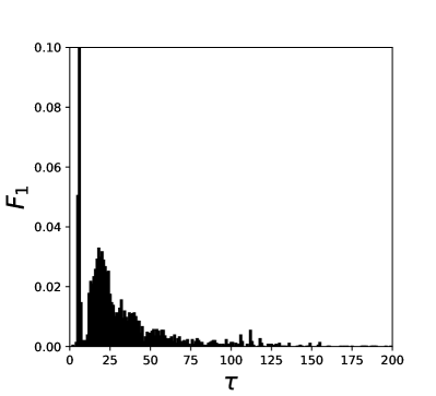
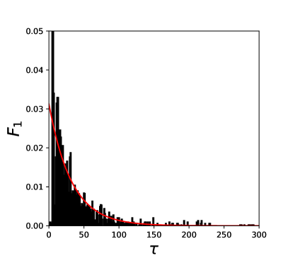
Figure 3: $F_{1}$ distribution with $\left|{\alpha}\right|^{2}=25$ and $\chi^{\prime}/\chi=10^{-3}$ for (a) coherent state and (b) even coherent state.

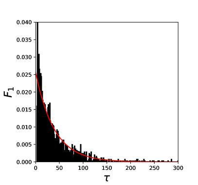
Figure 4: $F_{1}$ distribution with $\left|{\alpha}\right|^{2}=100$, $\chi^{\prime}/\chi=10^{-3}$ for (a) coherent state and (b) even coherent state.

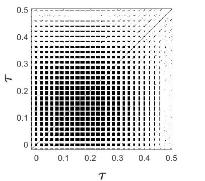
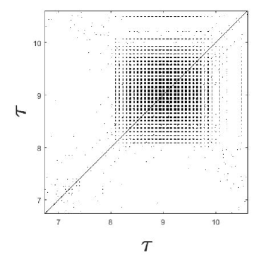
Figure 5: Recurrence plot for initial (a) coherent state and (b) even coherent state with $\left|{\alpha}\right|^{2}=25$ and $\chi^{\prime}/\chi=10^{-3}$ (the parameters are same as in Fig. 3).

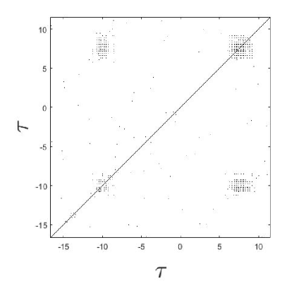
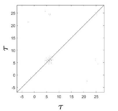
Figure 6: Recurrence plot for initial (a) coherent state and (b) even coherent state with $\left|{\alpha}\right|^{2}=100$, $\chi^{\prime}/\chi=10^{-3}$ (parameters are same as in Fig. 4).

Similarly, we have computed this quantity for even ($\ell=2$) and higher order superposition state. Fig. 3 compares the $F_{1}$ distribution for coherent state and even coherent state (Eq. 13) for $\left|{\alpha}\right|^{2}=25$ and ${\chi^{\prime}}/{\chi}=10^{-3}$ with $10^{6}$ data points and cell size between $10^{-3}$ and $10^{-2}$. The $F_{1}$ distribution for CS $\left|{\alpha}\right\rangle$, for small $\left|{\alpha}\right|^{2}$ is a discrete one with finite number of points which shows the quasi-periodic nature. If, instead we use even coherent state a decaying exponential distribution is obtained, which signifies a higher degree of mixing and the presence of ergodicity in the dynamics. This is more pronounced for larger value of $\left|{\alpha}\right|^{2}$, as may be seen in Fig. 4. Figures 5 and 6 depicts the recurrence plots corresponding to the $F_{1}$ distribution in Figs. 3 and 4 respectively. The regular patterned structure is a characteristic of quasi-periodicity with small number of incommensurate frequencies Marwan et al. (2007). The other recurrence plots signals the increase in the degree of mixing with superposition and with the increase in $\left|{\alpha}\right|^{2}$, corroborating our deduction based on $F_{1}$ distribution. Similarly higher order superposition is also analyzed and similar conclusion is drawn (not shown here).

III.2 Dynamics of superposition states in the bosonic Josephson junction

With the advent of Bose-Einstein condensate (BEC) of weakly interacting gases Anderson et al. (1995); Davis et al. (1995); Bradley et al. (1995), an experimental system has become available for the quantitative investigation of Josephson effects in a very well controllable environment. We have focused on bosonic Josephson junction, generated by confining single BEC in a double-well potential. We have considered the Bose-Hubbard Hamiltonian for N bosons in a two-site system.

$$H_{2}=-\dfrac{J}{2}({\hat{a}_{1}^{\dagger}}\hat{a}_{2}+\hat{a}_{1}\hat{a}_{2}^{\dagger})+\dfrac{U}{4}(\hat{a}_{1}^{\dagger}\hat{a}_{1}-\hat{a}_{2}^{\dagger}\hat{a}_{2})^{2},$$ (34)

where $a_{i}$ and $a_{i}^{\dagger}$ are the annihilation and creation operators respectively for the bosonic particle in $i^{th}$ mode. $J$ is the hopping amplitude describing the mobility of bosons and is the measure of coupling strength between the two modes and U, the interaction strength arising from the local interaction within the two wells. By defining the three $SU(2)$ generators, $L_{x}=(\hat{a}_{1}^{\dagger}\hat{a}_{2}+\hat{a}_{1}\hat{a}_{2}^{\dagger})/2$, $L_{y}=(\hat{a}_{1}^{\dagger}\hat{a}_{2}-\hat{a}_{1}\hat{a}_{2}^{\dagger})/2$ and $L_{z}=(\hat{a}_{1}^{\dagger}\hat{a}_{1}-\hat{a}_{2}\hat{a}_{2}^{\dagger})/2$, Eq. (34) can be expressed in the form

$$H_{2}=-JL_{x}+UL_{z}^{2}.$$ (35)

Most experiments on the bosonic Josephson system measures quantities defined via the expectation values of single particle Bloch vector such as $\dfrac{2\left\langle{L_{x}}\right\rangle}{N}$. The dimensionless parameter $u=\dfrac{NU}{J}$ is considered to study the system dynamics. We have taken $u$ such that it falls in the so-called Josephson regime $(1<u<N^{2})$. In the Josephson regime, the fluctuations in the atom numbers are reduced and the coherence is high.

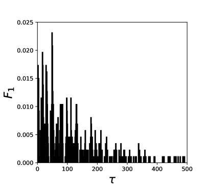
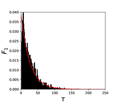
Figure 7: $F_{1}$ distribution for (a) pi state and (b) even state with $N=40$ and $u=50$.

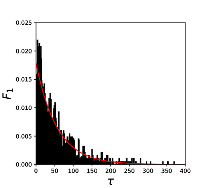
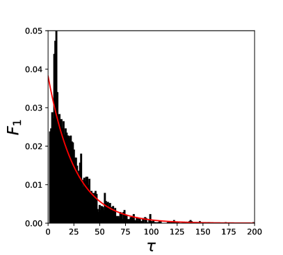
Figure 8: $F_{1}$ distribution for (a) pi state and (b) even state with $N=40$ and $u=90$.

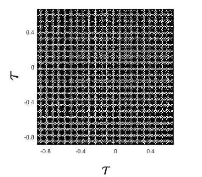
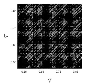
Figure 9: Recurrence plot for initial (a) pi state and (b) even state with $N=40$ and $u=50$ (the parameters are same as in Fig. 7).

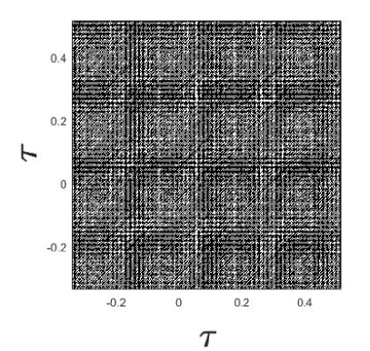
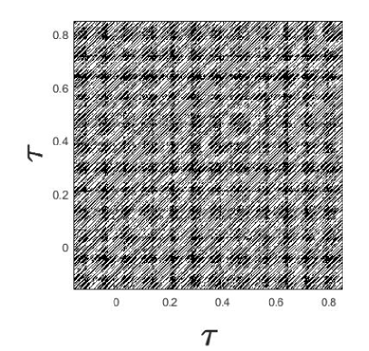
Figure 10: Recurrence plot for initial (a) pi state and (b) even state with $N=40$ and $u=90$ (the parameters are same as in Fig. 8) .

The dynamics of the system is carried out by considering $SU(2)$ coherent states and its superposition as initial state. $SU(2)$ coherent states are the eigenstates of angular momentum operator ${\hat{L}^{2}}$. In terms of angular momentum basis, $\left|{l;m}\right\rangle\equiv\left|{l+m,l-m}\right\rangle$ where $m$ varies from $-l$ to $l$, the $SU(2)$ coherent state can be written as

$$\left|{\theta,\phi}\right\rangle={} \Big{[}1+\text{tan}^{2}(\theta/2)\Big{]}^{-1}\sum_{m=-l}^{l}\Big{[}\text{tan}\left((\theta/2)e^{-i\phi}\right)\Big{]}^{l+m}$$ (36)

$$\times\binom{2l}{l+m}^{1/2}\left|{l;m}\right\rangle,$$

where $0<\theta<\pi$ and $0<\phi<2\pi$ are the rotation angles of the state $\left|{m=-l}\right\rangle$. In our study we have taken $\theta=\pi/2$, which corresponds to equal population in the two modes.

To study and analyze the difference in the dynamics of superposition states, we compare the $F_{1}$ distribution, recurrence plot and Lyapunov exponent for the states $\left|{\pi/2,\pi}\right\rangle$ (pi state) and $\dfrac{1}{\sqrt{2}}\big{(}\left|{\pi/2,0}\right\rangle+\left|{\pi/2,\pi}\right\rangle\big{)}.$ Depending on whether $l$ is even or odd the above superposition state can be called even or odd state $(l=N/2)$.
Figs. 7-10 compare the $F_{1}$ distribution and recurrence plot for pi state and even state with $N=40$ and $10^{6}$ data points. Fig. 7 depicts the $F_{1}$ distribution with $u=50$ and cell size of $10^{-2}$. The quasi-periodicity of the pi state is clear from the finite number of points in the $F_{1}$ distribution and the hyperbolicity and ergodicity in the dynamics is seen for the superposition (even) state which shows a decaying exponential spectrum. As $u$ value increases the ergodicity in the dynamics becomes more pronounced as clear from Fig. 8. The regular patterned structure in the recurrence plot in Fig. 9 is consistent with the $F_{1}$ distribution and the broken lines in the other recurrence plot signals the signature of chaos in the system. When we consider superposition states, more number of broken lines are visible in recurrence plots (Fig. 10) which indicates more chaoticity in the system. Lyapunov exponent for these are calculated and chaotic behaviour in the dynamics is confirmed with positive $\lambda$ and it is seen that $\lambda$ is larger for superposition states which is evident from Fig. 11 and Fig. 12. Other superposition states also gives similar difference in the dynamics from the non-superposed one.

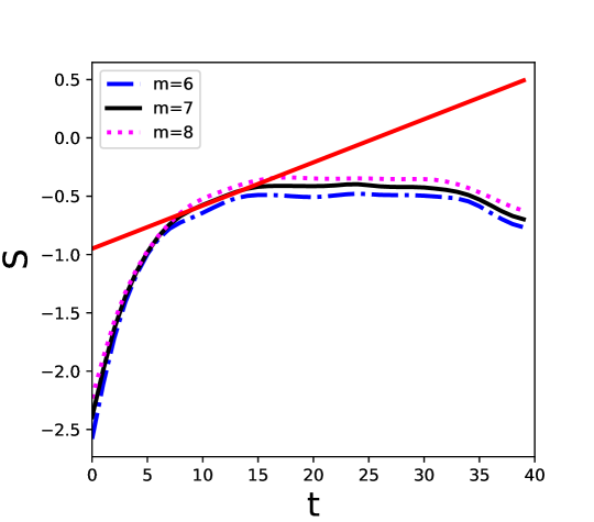
Figure 11: Plot to find the Lyapunov exponet ($\lambda$) for initial even state with $N=40$ and $u=50$ (parameters are same as in Fig. 9). Slope of the graph gives $\lambda=0.036$.

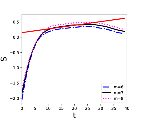
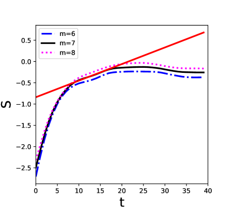
Figure 12: Plots to find the Lyapunov exponent for initial (a) pi state and (b) even state with $N=40$ and $u=90$ (the parameters are same as in Fig. 10). Slops of the graphs give $\lambda=$ (a) $0.012$ and (b) $0.039$.

IV Conclusion

We have studied the dynamics of superposition of wavepackets evolving under different nonlinear Hamiltonians corresponding to Kerr medium, Morse oscillator and bosonic Josephson junction. We have found that even the period of evolution changes when we consider different superpositions of states as initial states. Further, we have extended the study to find the consequence of superposition states on    the more complex dynamics such as quasi-periodic, ergodic and chaotic dynamics  using both qualitative and quantitative  methods in time series analysis. We have shown that the systems which are periodic  turned to quasi-periodic or ergodic   when we have changed the initial state from single wave packet to superposition of wave packets. Our results in this paper is a new direction in the theory of nonlinear dynamics in quantum systems because dynamical changes in the evolution of systems due to superposition of wavepackets are not reported in the literature earlier.

V Acknowledgement

M. R. acknowledges support by the Institute for Basic Science in Korea (IBS-R024-Y2).

References

- Dirac (1981) P. A. M. Dirac, The principles of quantum mechanics, 27 (Oxford university press, 1981).
- da Costa and De Ronde (2013) N. da Costa and C. De Ronde, Foundations of Physics 43, 845 (2013).
- Feix et al. (2015) A. Feix, M. Araújo, and Č. Brukner, Physical Review A 92, 052326 (2015).
- Bennett et al. (1992) C. H. Bennett, G. Brassard, and N. D. Mermin, Physical Review Letters 68, 557 (1992).
- Milburn and Braunstein (1999) G. Milburn and S. L. Braunstein, Physical Review A 60, 937 (1999).
- Ralph et al. (2003) T. C. Ralph, A. Gilchrist, G. J. Milburn, W. J. Munro, and S. Glancy, Physical Review A 68, 042319 (2003).
- Cerf et al. (2000) N. J. Cerf, A. Ipe, and X. Rottenberg, Physical Review Letters 85, 1754 (2000).
- Bužek et al. (1992) V. Bužek, A. Vidiella-Barranco, and P. L. Knight, Physical Review A 45, 6570 (1992).
- Gerry (1993) C. C. Gerry, Journal of Modern Optics 40, 1053 (1993).
- Yurke and Stoler (1986) B. Yurke and D. Stoler, Physical review letters 57, 13 (1986).
- Miranowicz et al. (1990) A. Miranowicz, R. Tanas, and S. Kielich, Quantum Optics: Journal of the European Optical Society Part B 2, 253 (1990).
- Paprzycka and Tanas (1992) M. Paprzycka and R. Tanas, Quantum Optics: Journal of the European Optical Society Part B 4, 331 (1992).
- Tara et al. (1993) K. Tara, G. Agarwal, and S. Chaturvedi, Physical Review A 47, 5024 (1993).
- Monroe et al. (1996) C. Monroe, D. Meekhof, B. King, and D. J. Wineland, Science 272, 1131 (1996).
- Ourjoumtsev et al. (2007) A. Ourjoumtsev, H. Jeong, R. Tualle-Brouri, and P. Grangier, Nature 448, 784 (2007).
- Gao et al. (2010) W.-B. Gao, C.-Y. Lu, X.-C. Yao, P. Xu, O. Gühne, A. Goebel, Y.-A. Chen, C.-Z. Peng, Z.-B. Chen, and J.-W. Pan, Nature physics 6, 331 (2010).
- Kirchmair (2013) G. Kirchmair, Nature (London) 495, 205 (2013).
- Von Neumann (1929) J. Von Neumann, Phys. Z. 30, 465 (1929).
- Peres (1984) A. Peres, Phys. Rev. A 30, 504 (1984).
- Goldstein et al. (2014) H. Goldstein, C. P. Poole, and J. L. Safko, Classical Mechanics: Pearson New International Edition (Pearson Higher Ed, 2014).
- Scott and Milburn (2001) A. Scott and G. J. Milburn, Physical Review A 63, 042101 (2001).
- Maletinsky et al. (2007) P. Maletinsky, C. Lai, A. Badolato, and A. Imamoglu, Physical Review B 75, 035409 (2007).
- Bettelheim et al. (2007) E. Bettelheim, A. G. Abanov, and P. Wiegmann, Journal of Physics A: Mathematical and Theoretical 40, F193 (2007).
- Wang et al. (2014) G. Wang, L. Huang, Y.-C. Lai, and C. Grebogi, Physical review letters 112, 110406 (2014).
- Mehta (2004) M. L. Mehta, Random matrices, Vol. 142 (Elsevier, 2004).
- Andreev et al. (1996) A. Andreev, O. Agam, B. Simons, and B. Altshuler, Physical review letters 76, 3947 (1996).
- Eckmann et al. (1987) J.-P. Eckmann, S. O. Kamphorst, and D. Ruelle, EPL (Eur ophysics Letters) 4, 973 (1987).
- Marwan et al. (2007) N. Marwan, M. C. Romano, M. Thiel, and J. Kurths, Physics reports 438, 237 (2007).
- Rosenstein et al. (1993) M. T. Rosenstein, J. J. Collins, and C. J. De Luca, Physica D: Nonlinear Phenomena 65, 117 (1993).
- Kantz (1994) H. Kantz, Physics letters A 185, 77 (1994).
- Sudheesh et al. (2009) C. Sudheesh, S. Lakshmibala, and V. Balakrishnan, Physics Letters A 373, 2814 (2009).
- Sudheesh et al. (2010) C. Sudheesh, S. Lakshmibala, and V. Balakrishnan, EPL (Europhysics Letters) 90, 50001 (2010).
- Shankar et al. (2014) A. Shankar, S. Lakshmibala, and V. Balakrishnan, Journal of Physics B: Atomic, Molecular and Optical Physics 47, 215505 (2014).
- Pradeep et al. (2020) A. Pradeep, S. Anupama, and C. Sudheesh, The European Physical Journal D 74, 3 (2020).
- Rohith and Sudheesh (2014) M. Rohith and C. Sudheesh, Journal of Physics B: Atomic, Molecular and Optical Physics 47, 045504 (2014).
- Rohith and Sudheesh (2015) M. Rohith and C. Sudheesh, Physical Review A 92, 053828 (2015).
- Robinett (2004) R. W. Robinett, Physics Reports 392, 1 (2004).
- Milburn (1986) G. J. Milburn, Physical Review A 33, 674 (1986).
- Kitagawa and Yamamoto (1986) M. Kitagawa and Y. Yamamoto, Physical Review A 34, 3974 (1986).
- Napoli and Messina (1999) A. Napoli and A. Messina, The European Physical Journal D-Atomic, Molecular, Optical and Plasma Physics 5, 441 (1999).
- Dodonov et al. (1974) V. Dodonov, I. Malkin, and V. Man’Ko, Physica 72, 597 (1974).
- Morse (1929) P. M. Morse, Physical Review 34, 57 (1929).
- Dong et al. (2002) S.-H. Dong, R. Lemus, and A. Frank, International Journal of Quantum Chemistry 86, 433 (2002).
- Ghosh et al. (2006) S. Ghosh, A. Chiruvelli, J. Banerji, and P. K. Panigrahi, Phys. Rev. A 73, 013411 (2006).
- Strekalov (2016) M. L. Strekalov, Journal of Mathematical Chemistry 54, 1134 (2016).
- Eckmann (1981) J. Eckmann, Rev. Mod. Phys. 53, 643 (1981).
- Hirata (1995) M. Hirata, “Dynamical systems and chaos,” (1995).
- Hirata (1993) M. Hirata, Ergodic Theory and Dynamical Systems 13, 533 (1993).
- Balakrishnan and Theunissen (2001) V. Balakrishnan and M. Theunissen, Stochastics and Dynamics 1, 339 (2001).
- Zbilut (1992) J. P. Zbilut, Physics letters A 171, 199 (1992).
- Wolf et al. (1985) A. Wolf, J. B. Swift, H. L. Swinney, and J. A. Vastano, Physica D: Nonlinear Phenomena 16, 285 (1985).
- Lakshmibala et al. (2011) S. Lakshmibala, V. Balakrishnan, and C. Sudheesh, Asian Journal of Physics 20, 181 (2011).
- Anderson et al. (1995) M. H. Anderson, J. R. Ensher, M. R. Matthews, C. E. Wieman, and E. A. Cornell, science , 198 (1995).
- Davis et al. (1995) K. B. Davis, M.-O. Mewes, M. R. Andrews, N. J. van Druten, D. S. Durfee, D. Kurn, and W. Ketterle, Physical review letters 75, 3969 (1995).
- Bradley et al. (1995) C. C. Bradley, C. Sackett, J. Tollett, and R. G. Hulet, Physical review letters 75, 1687 (1995).