Faint Stars in a Faint Galaxy: I. Ultra Deep Photometry of the Boötes I Ultra Faint Dwarf Galaxy

Abstract

We present an analysis of new extremely deep images of the resolved stellar population of the Boötes I ultra faint dwarf spheroidal galaxy. These new data were taken with the Hubble Space Telescope, using the Advanced Camera for Surveys (Wide Field Camera) and Wide Field Camera 3 (UVIS), with filters F606W and F814W (essentially V and I), as part of a program to derive the low-mass stellar initial mass function in this galaxy. We compare and contrast two approaches to obtaining the stellar photometry, namely ePSF and DAOPHOT. We identify likely members of Boötes I based on the location of each star on the color-magnitude diagram, obtained with the DAOPHOT photometry from the ACS/WFC data. The probable members lie close to stellar isochrones that were chosen to encompass the known metallicity distribution derived from spectroscopic data of brighter radial-velocity member stars and are consistent with the main-sequence turnoff. The resulting luminosity function of the Boötes I galaxy has a 50% completeness limit of 27.4 in F814W and 28.2 in F606W (Vega magnitude system), which corresponds to a limiting stellar mass of $\simlt 0.3{\cal M}_{\odot}$.

1 Introduction

The stellar initial mass function (IMF) describes the distribution of stellar masses formed in any single star formation event (Salpeter, 1955). Determinations of the IMF for star clusters and field stellar populations of the Milky Way Galaxy, over a range of ages and metallicities, have found the IMF to be consistent with being invariant, and well fit by a broken power law or a lognormal distribution (see, for example, the recent analysis of Sollima 2019 and the reviews of Kroupa 2002, Chabrier 2003, Bastian et al. 2010 and Kroupa et al. 2013). Whether or not the IMF for other galaxies is the same as that of the Milky Way has been the subject of much recent debate (cf. Bastian et al. 2010). Understanding if, and how, the IMF changes is crucial to many areas of astrophysics, from stellar-mass estimates of high-redshift galaxies, to models of stellar feedback in simulations of galaxy formation. The nearby low surface-brightness satellite galaxies of the Milky Way are obvious targets for study of the IMF, particularly since their low mean metallicity and high inferred dark-matter content provides an environment very different from the local disk. Galaxies whose stellar populations have a narrow range of ages offer the cleanest case studies. The luminosity function of the lower main sequence, below the old(est) turnoff, can be transformed into the IMF, modulo corrections for unresolved binary systems, possible mass-dependent dynamical effects and observational incompleteness. The high-mass IMF in self-enriched systems can be constrained by the elemental abundances of the most metal-poor stars (cf. Wyse & Gilmore 1992; Wyse 1998).

Grillmair et al. (1998), in a pioneering study, obtained imaging data with the Hubble Space Telescope (HST) that reached 3 magnitudes below the old main-sequence turnoff in the Draco dwarf spheroidal (distance $\sim 80$ kpc). They determined the luminosity function of stars in Draco around the turn-off region, corresponding to a stellar mass range of $0.6\simlt{\cal M/M_{\odot}}\simlt 0.9$, and found that it was very similar to that in the old, metal-poor Milky Way globular cluster M68. They also found that their data were consistent with an underlying power-law IMF, with slope similar to that of the IMF derived for stars in the solar neighborhood. Feltzing et al. (1999) obtained deeper data with HST for the somewhat closer, but similarly old and metal-poor, Ursa Minor dSph (hereafter UMi, distance $\sim 66$ kpc). Their color-magnitude data extend more than 4 magnitudes below the main-sequence turnoff and, similarly as found for Draco, the luminosity function of the stars in UMi was found to be indistinguishable from that measured for an old, metal-poor Milky Way globular cluster (M92), in this case down to a magnitude corresponding to mass $\sim 0.45{\cal M_{\odot}}$. The subsequent analysis of the full deep HST data for UMi, in Wyse et al. (2002), extended the luminosity function to reach a corresponding mass $\sim 0.3{\cal M_{\odot}}$ and again found excellent agreement between the luminosity functions of UMi and old, metal-poor Milky Way globular clusters (M92 and M15). The age and (mean) metallicity of the stellar population in UMi are the same as those of M92 and M15, so that provided internal and external dynamical effects may be neglected for the globular cluster data (as argued by those authors), a comparison of the luminosity functions is equivalent to a comparison of the IMFs. The inferred IMF for the Draco dSph and that for the UMi dSph are also in good agreement, over the limited mass range in common.

The discovery of Ultra Faint Dwarf galaxies (UFDs, galaxies with $L<10^{5}L_{\odot}$, see reviews of Belokurov 2013; Simon 2019) allowed the exploration of the IMF in even lower luminosity, more dark-matter dominated systems. Geha et al. (2013) targeted two UFDs, Hercules and Leo IV, at distances of 135 pc and 156 kpc, respectively. The data allowed investigation of the IMF in each UFD over the mass range $0.5\simlt{\cal M/M_{\odot}}\simlt 0.8$. Comparison with the published low-mass IMF slopes for the three other galaxies with deep star-count data (the Milky Way, the Small Magellanic Cloud and UMi) led Geha et al. (2013) to conclude that the low-mass end of the IMF varied systematically across the sample, in the sense that the galaxies with lower metallicity, or with lower stellar velocity dispersion, had a more bottom-light IMF. Gennaro et al. (2018) reanalyzed the data for the two UFDs and expanded the sample with the addition of 4 more (Coma Berenices, Ursa Major I, Canes Venatici II, and Boötes I - hereafter Boo I). Their results provided more evidence for a bottom-light low-mass IMF in UFDs compared to the Milky Way, albeit that the quoted significance of the variation depended on the adopted form of the IMF (typically $\sim 95$% for a power-law, $\sim 68$% for a log-normal mass function).

Indeed, the robustness of any conclusions as to the variability of the IMF with these data, which cover only the mass range $0.5\simlt{\cal M}/{\cal M_{\odot}}\simlt 0.8$ (the upper limit being set by the main-sequence turn-off), was investigated by El-Badry et al. (2017). Those authors concluded that it would be necessary to obtain data that reached down to masses below $\sim 0.3{{\cal M_{\odot}}}$, a limit met by only the UMi dataset of Wyse et al. (2002), for the extragalactic systems studied thus far and discussed above.

This paper is the first in a series describing the results of our program to determine the low-mass IMF down to $\simlt 0.3{\cal M_{\odot}}$ in the UFD Boo I and revisit the issue of possible variability of the IMF. This present paper focuses on the more technical aspects of the data analysis, as we aim to push the luminosity function as faint as possible. We begin, in Section 2, with a brief motivation for the choice of Boo I. We then (Section 3) describe the new observational data, taken with the Hubble Space Telescope (HST) under program GO-15317 (PI I. Platais), together with archival data that we use as an off-field. We adopted two approaches to the photometric reductions (ePSF and DAOPHOT) and illustrate the relative strengths of each, as described in Section 4. Our science goal requires pushing the data to their faintest limits, which in turn requires a thorough understanding of possible systematics. We therefore document in some depth the detailed procedures we used. Our approach to the determination of the likelihood of membership of Boo I for the stars in our sample is presented in Section 6, together with the resulting cleaned color-magnitude diagram of likely members. We close, in Section 7, with a brief discussion of the achieved lower-mass limit and the next steps in the later papers in this series.

2 Boötes I Ultra Faint Dwarf Galaxy

Boo I was discovered by Belokurov et al. (2006b) in the Sloan Digital Sky Survey imaging data. This system is relatively luminous, with $L_{V}\sim 3\times 10^{4}L_{\odot}$ (Martin et al., 2008; Okamoto et al., 2012) and is at a distance of $\simlt 65$ kpc, comparable to the distance of UMi, and thus is significantly closer than the other UFDs of comparable luminosity studied by Geha et al. (2013) and Gennaro et al. (2018), which are located beyond 100 kpc. Such a combination of brightness and closeness is beneficial for pushing the stellar luminosity function to the required faint limits. The previous HST observations of Boo I (GO-12549, P.I. T. Brown), used in Gennaro et al. (2018), reached an approximate fifty percent completenes limit at magnitudes corresponding to $\sim 0.5{\cal M_{\odot}}$ and our intention is to reach $\sim 0.3{\cal M_{\odot}}$.

The stellar population of Boo I is old and metal-poor and its color-magnitude diagram is very similar to that of the globular cluster M92 (Belokurov et al., 2006b). Boo I has been the target of several spectroscopic and imaging surveys and its basic properties are given in Table 1. The wide-area imaging surveys found that Boo I is somewhat elongated, with an ellipticity $\epsilon\sim 0.2-0.3$ (Belokurov et al. 2006b, Martin et al. 2008, Okamoto et al. 2012, Roderick et al. 2016, Muñoz et al. 2018a), and has extended stellar substructure, most recently quantified by Roderick et al. (2016). The proper motion of Boo I has been derived from Gaia DR2 (Gaia Collaboration et al., 2018), with the most recent analysis (Simon, 2018) giving $\mu_{\alpha}cos\delta=-0.472\pm 0.046~{}\text{mas}\text{yr}^{-1}$, $\mu_{\delta}=-1.086\pm 0.034~{}\text{mas}\text{yr}^{-1}$. The corresponding orbital motion has a pericenter of greater than 30 kpc (e.g. $45\pm 5$ kpc; Simon, 2018) which is large enough that Galactic tidal forces have probably not been important in sculpting the stellar content.

Table 1: Properties of Boo I

Parameter	Value	Reference
RA (J2000)	14:00:06	1
Dec (J2000)	+14:30:00	1
$\ell$	$358^{\circ}.1$	1
b	$69^{\circ}.6$	1
$A_{V}$	0.047	2
$r_{h}$ (exponential)	$12\arcmin.8\pm 0\arcmin.7$	3
$\epsilon$	0.22	3
Position Angle	$14^{\circ}.2$	3
$M_{V}$	$-5.92{\pm 0.2}$	3
$(m-M)_{0}$	$18.96\pm 0.12$	4
Distance	$62\pm 4$ kpc	4
$\langle\ {\rm[Fe/H]}\ \rangle$	$-2.55$	5, 6
$\Delta{\rm[Fe/H]}$	1.70	5
Age	$\sim 13$ Gyr	1, 3, 7

Note. — References: (1) Belokurov et al. (2006b), (2) Schlafly & Finkbeiner (2011), (3) Okamoto et al. (2012), (4) Siegel (2006), (5) Norris et al. (2010b), (6) Gilmore et al. (2013), (7) Brown et al. (2014)

Spectroscopic studies have established that the iron-abundance distribution peaks at ${\rm[Fe/H]}\sim-2.5$, with a metal-poor tail extending to ${\rm[Fe/H]}\sim-3.5$ and a sharp decline more metal-rich of the peak, to ${\rm[Fe/H]}\sim-1.8$ (Norris et al. 2010b, see also Norris et al. 2008, Lai et al. 2011, Brown et al. 2014). Analyses of samples with high-resolution spectroscopy, and thus abundances for individual elements, find a range in ${\rm[\alpha/Fe]}$, from $\sim 0.1$ to $\sim 0.5$ (Feltzing et al., 2009) consistent with a modest trend of increasing ${\rm[\alpha/Fe]}$ with decreasing [Fe/H] (Gilmore et al. 2013, Ishigaki et al. 2014, Frebel et al. 2016). This trend suggests that the duration of star formation in Boo I was long enough for gas to be enriched by Type Ia supernovae, as discussed in Gilmore et al. (2013) and Frebel et al. (2016). The delay-time distribution for Type Ia supernovae is a topic of some debate and, in a further complication, sub-Chandrasekhar mass explosions have been implicated in the early iron enrichment of dSph (de los Reyes et al., 2020). The minimum time for the onset of the incorporation of iron from a double-degenerate binary is expected to be $\simgt 10^{8}$ yr (e.g. Smecker & Wyse, 1991), while the reported age distribution of stars in Boo I, estimated from the spread in color of the turn-off region, has 97% with an age of 13.3 Gyr and 3% with an age of 13.4 Gyr (on a scale with the age of M92 being 13.2Gyr; Brown et al., 2014). We will revisit the possible age range of the stars in Boo I in paper III of this series.

The range of chemical abundances apparent in the members of Boo I is expected to lead to a broadening, in color, of the main sequence, particularly below $\sim 0.5{\cal M_{\odot}}$, reflecting changes in the dominant source of opacity for these cool stars (as discussed in e.g. Allard et al. 1997 and Baraffe et al. 1997). This enhanced broadening for the lower main sequence is compounded, in the observational dataset presented here, by the larger photometric errors for fainter sources. Knowledge of the elemental abundance distributions from complementary data, such as for Boo I, is an important element in the choice of target galaxy.

3 Observations

We obtained deep photometry of the Boo I  UFD, with the aim of pushing the faint magnitude limit below that achieved in earlier datasets, and thus extending the stellar mass regime available for study of the IMF. The new observations for this project were taken during twenty-six orbits of HST from May 30th to July 5th, 2019, utilizing the Advanced Camera for Surveys (ACS) as primary instrument and the Wide Field Camera 3 (WFC3) in parallel mode. The ACS observations were taken with the Wide Field Camera (WFC), and the WFC3 observations were taken with UVIS. For future reference, the field of view of ACS/WFC is $202^{\prime\prime}\times 202^{\prime\prime}$, with a resolution of $0.05~{}\text{arcsec}~{}\text{pix}^{-1}$, while the field of view of WFC3/UVIS is $162~{}\arcsec\times 162\arcsec$, with a resolution of $0.04~{}\text{arcsec}~{}\text{pix}^{-1}$. Twenty-four orbits were dedicated to on-target observations of Boo I – more than four times the exposure time of the previous deep observations of Boo I – with the remaining two orbits dedicated to an off-field. The data described here may be obtained from the MAST archive at https://dx.doi.org/10.17909/t9-jr7h-en65 (catalog doi:10.17909/t9-jr7h-en65).

The on-field observations were taken in three pointings, the footprint of which is indicated in Figure 1. The ACS/WFC fields match three of those observed with ACS/WFC by GO-12549; this allows for the possibility of a deep proper-motion study, the topic of a future paper. We also selected the same ACS/WFC filters as this earlier work, namely F606W and F814W, and the equivalent passbands for the parallel observations with WFC3/UVIS. The ACS/WFC fields selected were pointings one, three, and five of GO-12549 and we retained their naming convention, so that pointing three encompasses the central regions of Boo I (see Table 2 for the coordinates of the field centers). As detailed in Table 2, each field of Boo I was imaged over four orbits in each filter, and two exposures were taken per orbit. A four-point dither pattern was used to mitigate the effects of the under-sampled point spread function (PSF) of the instruments on HST (see Lauer, 1999a, b for more discussion). The dithering strategy also optimized the rejection of detector artifacts and cosmic rays. One of the two guide stars used to obtain fine-lock guiding of the telescope could not be acquired for orbit 10, during observations of pointing one. The availability of only one guide star resulted in some loss of astrometric accuracy during this orbit, but happily there was no degradation in image quality.

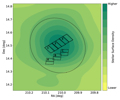
Figure 1: The footprint of the observed fields of Boo I. The solid rectangles closest to the center represent the ACS/WFC fields, and the dotted rectangles represent the parallel WFC3/UVIS fields. The naming schema of our pointings is East to West, i.e. pointing 1 of the ACS/WFC observations and pointing A of the WFC3/UVIS observations are Eastmost. The green contours indicate the stellar surface density, which we created from the photometry published in Muñoz et al. (2018b). The dashed oval represents the half-light (elliptical) radius from Okamoto et al. (2012), corresponding to $\sim 230$ pc at an assumed distance of 62 kpc.

The off-field was imaged for one orbit in each filter, with only one exposure. The off-field data are intended to aid in the quantification of the contribution of background unresolved galaxies and non-member stars to the Boo I fields. As discussed in Section 4.7, this one long exposure proved to be difficult to clean. We therefore searched the MAST archive and identified a dataset to use as a second off-field, with Galactic coordinates similar to those of Boo I, and with multiple-exposure ACS/WFC imaging in the same filters (designated ‘Off Field 2’ in Table 2).

As noted in Section 1, our aim of determining the low-mass stellar IMF places stringent requirements on the data analysis, and the following two sections are, by necessity, technical. Readers who are less interested, or who are very familiar with the photometric reduction techniques, may prefer to turn to Section 6 where the resultant deep color-magnitude diagrams are presented.

Table 2: Details of the observations

Pointing	Instrument	Filter	$\alpha_{2000}$	$\delta_{2000}$	Start UT Date	$N_{exp}$	Total Exp. Time
			[hh:mm:ss]	[∘:′:″]	[yymmdd]		[seconds]
Pointing 1	ACS/WFC	F606W	14:00:15.510	+14:28:42.06	190530	8	9792
Pointing 1	ACS/WFC	F814W	14:00:15.510	+14:28:42.06	190530	8	10064
Pointing 3	ACS/WFC	F606W	14:00:04.680	+14:30:47.17	190630	8	9792
Pointing 3	ACS/WFC	F814W	14:00:04.680	+14:30:47.17	190630	8	10064
Pointing 5	ACS/WFC	F606W	13:59:53.847	+14:32:52.28	190610	8	9792
Pointing 5	ACS/WFC	F814W	13:59:53.847	+14:32:52.28	190610	8	10064
Off Field	ACS/WFC	F606W	13:59:54.030	+15:57:45.65	190619	1	2603
Off Field	ACS/WFC	F814W	13:59:54.030	+15:57:45.65	190619	1	2660
Pointing A	WFC3/UVIS	F606W	14:00:17.882	+14:22:49.28	190530	8	10112
Pointing A	WFC3/UVIS	F814W	14:00:17.882	+14:22:49.28	190530	8	10312
Pointing B	WFC3/UVIS	F606W	14:00:07.053	+14:24:54.39	190630	8	10112
Pointing B	WFC3/UVIS	F814W	14:00:07.053	+14:24:54.39	190630	8	10312
Pointing C	WFC3/UVIS	F606W	13:59:56.221	+14:26:59.50	190610	8	10112
Pointing C	WFC3/UVIS	F814W	13:59:56.221	+14:26:59.50	190610	8	10312
Off Field 2	ACS/WFC	F606W	14:10:38.005	-11:43:58.62	140713	4	2080
Off Field 2	ACS/WFC	F814W	14:10:38.005	-11:43:58.62	140713	4	2110

4 Photometry: ACS/WFC Data

Photometry for the ACS/WFC on-field exposures was produced using two different techniques and software packages. The first, ePSF, developed by Anderson & King (2006), is an empirical approach that is able to map, with high fidelity, the changes in the true PSF across the CCD chip. ePSF photometry can be performed only on individual exposures, which results in a brighter detection limit than with co-added exposures. The second photometry software package that we employed is the stand-alone DAOPHOT II (Stetson, 1987) provided through Starlink (Currie et al., 2014). DAOPHOT can be run on drizzle-combined images from multiple dithered exposures, which allows for a deeper detection limit. The single images for each pointing and filter were combined through DrizzlePac, as described in detail in Section 4.2. In contrast to the empirical ePSF, the PSF fitting routine within DAOPHOT creates analytical models, which may not be flexible enough to capture the variation of the under-sampled PSF across the detector chip. We performed photometry using both ePSF and DAOPHOT to quantify how well their results compare, and to understand what impact the reduced flexibility of DAOPHOT had on the final photometry. The resulting photometric catalogs are compared in Section 4.6.

4.1 ePSF Photometry of ACS/WFC

Anderson & King (2000) developed the effective PSF (ePSF) techniques to measure accurate stellar positions and magnitudes for HST WFPC2 images, where the PSF was severely under-sampled and varied across the CCD chips. This approach was extended to ACS/WFC observations by Anderson & King (2006). Further improvements include corrections for the effective area of each pixel (i.e. the pixel area map) that preserve the photometric accuracy (Ryon et al., 2019). A detailed description of the ePSF technique may be found in Anderson et al. (2008a, b) and a short overview follows.

In the ePSF approach, the PSF is derived empirically by evaluation and scaling of the observed pixel intensity values. No analytical function is fitted, in contrast to the PSF fitting methods used within DAOPHOT (Stetson, 1987), DoPHOT (Schechter et al., 1993), or DOLPHOT (Dolphin, 2016). The variations of the PSF across each detector chip is represented by an array of fiducial PSFs, between which each star’s PSF is interpolated (Anderson & King, 2006). The variation of the PSF with time, due to, for example, telescope breathing or small changes in focus, is presented within ePSF as a spatially constant perturbation to the PSF for each image. A $5\times 5$ pixel inner box is used to construct the ePSF for the brightest pixels of each detected point source, an area that contain most of the flux. The code returns, for each individual exposure, a list of precise measurements of the stellar centroids, given as the X and Y positions in the detector coordinate system. These are then corrected for geometric distortions. The flux in counts, ${\rm flux_{DN}}$, is converted into instrumental magnitudes by applying the standard expression: $2.5\log{(\rm flux_{DN})}$. The code also returns a quality-of-fit parameter, qfit, which is used to separate stars with well-measured empirical PSFs from spurious detections, such as cosmic rays or hot pixels.

ePSF photometry was carried out on each single exposure of the ACS/WFC fields. Only measurements with $0<\textit{qfit}<0.5$ were selected for further examination. The distortion-corrected X and Y positions from each exposure in the F814W and F606W filters were then matched to the positions from the central exposure with respect to which the other exposures were dithered. A matching tolerance of $<0.1$ pixels in each of the X and Y coordinate allowed for the rejection of any remaining spurious detection in the individual exposures.

Finally, three corrections were applied to convert the photometric measurements from the individual images to the Vega magnitude system:

1. an empirical aperture correction from the ePSF radius out to a radius of 10 pixels ($0.5\arcsec$ on the individual exposures). The value of this correction was found by calculating the difference between the ePSF photometry and aperture photometry done using a 10-pixel radius, for isolated, well-exposed stars on drizzle-combined images. This correction is small, ranging from $\sim 0.02$ to $\sim 0.03$ magnitudes in the different filters;

2. an aperture correction from 10 pixels to infinity, using the encircled energy estimate provided in Bohlin (2016);

3. the filter-dependent Vega magnitude zero point for the observation date of each pointing

The final photometry for each star was calculated as a weighted average of the ePSF measurements from each individual exposure. The photometric error in each filter was estimated by the root-mean-square deviation of the independent measurements for each star. The final photometric catalog for each pointing provides X and Y positions, based in the detector reference frame, and weighted photometry in the F606W and F814W filters. We restricted the catalog to only sources that were present in at least three exposures per filter, which further ensured high-quality photometry. The resulting color-magnitude diagram from the ePSF photometry for each individual pointing is presented in Figure 2.

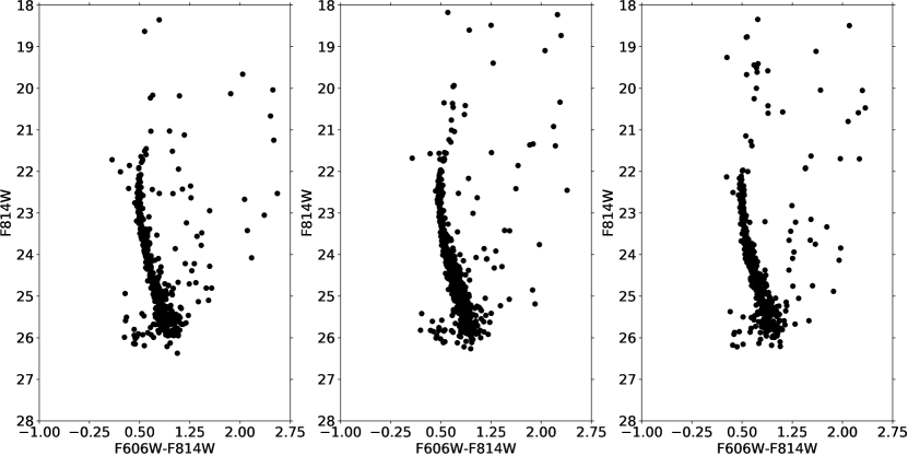
Figure 2: Color-magnitude diagram obtained from ePSF for all three on-field ACS/WFC pointings of our program. Only the photometry for sources present in at least three exposures per filter is presented. The relative number of detections in each pointing are broadly consistent with what one would anticipate from the surface density contours seen in Figure 1. Pointing one contains 484 sources and is leftmost, pointing three contains 588 sources and is central, and pointing five contains 501 sources and is rightmost. The main-sequence of Boo I  is well delineated down to a F814W magnitude of $\sim 25$.

4.2 DrizzlePac Aligning and Combining

As noted above, the PSF of HST instruments is under-sampled and varies spatially. The HST software DrizzlePac (STScI  Development  Team, 2012) was designed to rectify and combine dithered HST images into a common frame and, consequentially, enhance the spatial resolution and deepen the detection limit. The Mikulski Archive for Space Telescopes (MAST) provides users with images for each field of a given program that have already been combined using DrizzlePac, adopting default values for the parameters of this package. However, employing custom parameters (as described below) is recommended to exploit the full capabilities available through the drizzling algorithm, and improve accuracy of photometry. DrizzlePac also produces bad-pixel maps and cosmic-ray masks, allowing for the identification of problematic pixels that should be down-weighted during the combining process. The final, combined images are cosmic-ray cleaned, sky-subtracted, undistorted, free from detector artifacts, and, depending on dithering pattern, free from chip gaps, as is the case for the images analyzed in this paper. These final drizzle-combined images also have improved resolution and depth compared to the input individual images.

We used DrizzlePac version 2.2.6 to distortion-correct, align, and combine the individual exposures. The DrizzlePac task TweakReg was used to align the images and update the WCS information in the headers of the input images. TweakReg finds sources in each image, corrects for distortion (Kozhurina-Platais et al., 2015), calculates shift, rotation and scale, and aligns to a specified reference image. All images taken in the same filter at each pointing were aligned to one another utilizing the ‘general’ (i.e. six linear parameter) transformation. The F606W and F814W exposures were then aligned to each other, allowing for easier subsequent matching of detections between images. The aligned ACS/WFC images were then combined with the DrizzlePac task AstroDrizzle, adopting the parameter values final_pixfrac = 0.8 and final_scale = $0.04\arcsec/$pixel. These parameters and their definitions are discussed in depth in the DrizzlePac resources provided by STScI and in Gonzaga & et al. (2012) and Avila et al. (2015). Briefly, the value of final_pixfrac corresponds to the amount that each input pixel is shrunk before being added to the final pixel plane, where $\textit{final\textunderscore pixfrac}=0$ is equivalent to interlacing of pixels, and $\textit{final\textunderscore pixfrac}=1$ is equivalent to shifting and adding the pixels. The final_scale parameter represents the scale of the output pixel, where the native ACS/WFC pixel scale is $\sim 0.05\arcsec/$pixel. A side-by-side comparison of a portion of a distortion-corrected individual ACS/WFC exposure (i.e. the “single drizzled” image) from one pointing with the final, aligned and drizzle-combined image for the same pointing shown in Figure 3. The resolution has been noticeably improved, faint background galaxies are more distinguishable, and cosmic rays, hot pixels, and the chip gap were all removed. The final step was to mask large, over-exposed stars and galaxies, achieved using imedit within IRAF (Tody, 1986, 1993).

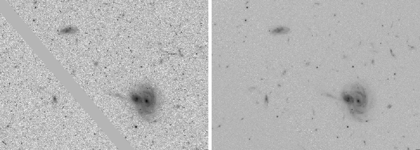
Figure 3: A side-by-side comparison of a single drizzled image, left, with a drizzle-combined image, right, for pointing 5 (the westmost) of the ACS/WFC observations. These exposures are in filter F606W, with an individual exposure time of 1,224 seconds and a combined total exposure time of 9,792 seconds. Note the increased resolution in the drizzled product, as well as the uniform sky and clean removal of cosmic rays. The region shown is centered on $13:59:55.2,+14:33:27.0$ and is $\sim 45\arcsec\times 32\arcsec$.

4.2.1 Spatially Resolved Background Galaxies

The data acquired in this program may be of interest for investigations of the stellar content of more distant galaxies than Boo I. The depth reached is intermediate between that of the COSMOS HDF fields and that of the Ultra Deep Field (HUDF), albeit in only two filters. The morphology of intermediate-redshift, spatially resolved galaxies may be studied in detail. For example, the left panel of Figure 4 shows a zoom-in on the prominent pair of spiral galaxies seen in Figure 3. There is a wealth of internal structure in each galaxy, and possible tidal features. The right panel shows a cutout of the same area of sky from the SDSS imaging data; the two galaxies are blended and only one source is identified, SDSS J135954.62+143321.8, with a reported photometric redshift of $0.42$.

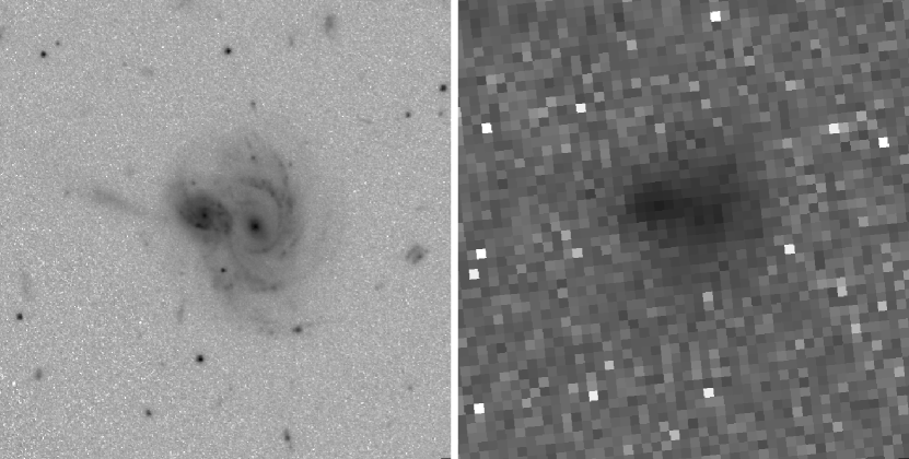
Figure 4: Left Panel: A zoom-in on the spiral galaxies seen in the drizzle-combined image from Figure 10 Right Panel: The same galaxies in the SDSS imaging data. The internal structure of both galaxies is resolved in the drizzle-combined image, with spiral arms, central concentrations and possible tidal features all evident. The SDSS image quality is insufficient to decompose the light into two galaxies and the source is identified as galaxy J135954.62+143321.8, at a photometric redshift of 0.42. The region shown is centered on 13:59:54.69, +14:33:21.4, and is $\sim 19\arcsec\times 15\arcsec$.

4.3 DAOPHOT Photometry

Aperture and PSF fitting photometry were performed with the DAOPHOT II package (Stetson, 1987). The rationale for choosing DAOPHOT II was twofold, owing to both its strong performance at detecting faint stars in low signal-to-noise data and its ability to be run on drizzle-combined images. The spatial variation of the PSF can be modeled within the DAOPHOT II package up to a quadratic function. The implementation of DAOPHOT on drizzled images requires that the data be in units of electrons and that the sky background be added back in. After such preparation of the ACS/WFC images for this project, sources for photometry were identified at a brightness threshold of four standard deviations above the sky background. These sources were then passed on to aperture photometry, and then to PSF fitting.

The PSF in each pointing was modeled within DAOPHOT by fitting a Penny function to well-exposed, isolated, stars, adopting a value of 10 pixels (corresponding to $0.4\arcsec$ after drizzling) for the ‘PSF radius’ and 3 pixels for the ‘fitting radius’ (also referred to as the ‘inner radius’). The Penny function (Penny & Dickens, 1986) was chosen for its flexibility and success in fitting the PSF of our drizzle-combined images. We tested all PSF functional forms available in DAOPHOT, and found that the Penny function produced the lowest $\chi$-squared goodness of fit value in the PSF fitting routine. The PSF photometry was obtained with the AllStar routine within DAOPHOT. This routine first fits the stars in the source list with a PSF, then subtracts those stars from the frame. The star-subtracted image was then run through the source finding, aperture photometry, and AllStar routines again, to detect and PSF-fit fainter stars. This iteration retrieved only $\sim 12\%$ as many stars as were retrieved in the first run and this low incremental yield led us to truncate the process after two runs. This decision was supported by the results of the artificial star tests, as discussed in Section 4.5 below, which found a maximum of one additional (artificial) star in the second round of AllStar.

The resulting PSF-fitted photometry was then converted to the Vega magnitude system, following a procedure similar to that used in the ePSF photometry, namely:

1. apply an aperture correction out to 10 pixels ($a_{3\rightarrow 10}$), again using the difference between the aperture and PSF instrumental photometry for well-exposed stars. The DAOPHOT routine Aperture was used to determine the magnitude of each given star, within a 10-pixel aperture, in the drizzle-combined images

2. apply an aperture correction from ten pixels to infinity ($a_{10\rightarrow\infty}$), from Bohlin (2016)

3. add the Vega magnitude zero point ($Z_{p}$) for the observation date and filter

4. subtract the DAOPHOT zero point ($C$), which is equal to 25 (Stetson, 1987)

5. account for the exposure time ($t_{e}$) by adding $2.5\log(t_{e})$, since the drizzle-combined images are in units of electrons, not electrons per second

The final expression for magnitude conversion is thus: $m_{DAOPHOT}=m_{psf}-a_{3\rightarrow 10}-a_{10\rightarrow\inf}+Z_{p}-C+2.5\log({t_{e}})$, where $m_{psf}$ is the DAOPHOT instrumental PSF magnitude. The error budget for each star is dominated by the standard error provided by DAOPHOT and the error bars shown in the color-magnitude plots below are calculated as the median of each of the standard error in color and magnitude, in magnitude bins of width $0.2$ mag.

4.4 Extinction Correction

We estimated the Galactic interstellar extinction using the dust maps from Schlafly & Finkbeiner (2011) and the ratio between extinction at the effective wavelength of our passbands and extinction in the Johnson V band . The reddening and extinction varies less than 0.005 magnitudes across the full areal coverage of the data and we adopted a uniform value of ${\rm A_{V}}=0.047$, equal to that for the nominal center of Boo I and assumed that the reddening and extinction does not vary across our field of view. We did not correct for any possible extinction due to dust within Boo I, as significant amounts of dust are unlikely to be present, given the low value of the upper limit on HI gas content of $<1.8\times 10^{3}{\cal M_{\odot}}$ (Grcevich & Putman, 2009). The resultant extinction correction is quite small, 0.04 magnitudes in F606W and 0.03 magnitudes in F814W. Note that in all of the comparisons below between the photometric data and theoretical isochrones, it is the isochrones that have been shifted to account for the dust reddening and extinction.

4.5 Artificial Star Tests: Completeness and Cleaning

Artificial star tests were carried out using the DAOPHOT AddStar routine. Three hundred artificial stars, at brightnesses that randomly sampled the entire magnitude range of the data, were placed at random locations within each frame, and the resulting file was run through the photometry pipeline. We did this thirty times per exposure per filter, giving a total of $54,000$ artificial stars added over 180 images. We chose to add this number of stars (300) in order to avoid noticeably altering the level of crowding, or overall surface density of sources, in the original exposures, while keeping the number of new frames produced to a manageable size. The total number of artificial stars added per filter is $\sim 10\times$ the number of stars in the final, cleaned photometric catalog, above the 50% completeness limit derived below (a total of 2,654 stars).

The approach we used to clean the data of spurious, non-stellar detections that had made it through the photometry pipeline is similar to that described by Okamoto et al. (2012). The stars retrieved from the artificial star tests were used to establish the statistical properties that a perfect stellar PSF would have, after being retrieved through the pipeline. Detected sources with properties that fell too far from those of this ideal point source were then discarded. The properties that formed the basis for this discrimination between stars and artefacts were both the value of the DAOPHOT sharp parameter, which describes the difference between the width of the object and the width of the PSF, and the fractional error in the magnitude.

A true stellar source should have a sharp parameter with value close to zero. The solid (red) curves in the lower panel of Figure 5 indicate the $\pm 3\sigma$ bounds from the artificial star tests in the F606W images, derived from the mean and standard deviation computed in bins of 0.05 magnitudes. The fractional error on magnitude was obtained as the ratio of the standard error of the magnitude quoted by DAOPHOT and the instrumental, DAOPHOT PSF magnitude. Again, the mean and standard deviation were computed within bins of 0.05 magnitude for the artificial stars retrieved from the tests, and the solid (red) curve in the upper panel of Figure 5 represent the $+3\sigma$ bound. The real sources detected by DAOPHOT are represented by the points in both panels of Figure 5. Those sources that lie within $3\sigma$ of the mean defined by the artificial stars are denoted by the filled circles and retained in the sample as likely stars, while sources that are rejected by one or other of these criteria (in each filter) are denoted by plus signs. The sources that pass this cleaning process have a mean and median goodness-of-fit parameter from DAOPHOT ($\chi$, related to the noise statistics) of approximately unity, as true stellar objects should. A total of 3,035 stars pass through this step, out of an original 8,383 detections and 2,654 stars have apparent magnitudes above the fifty percent completeness limit (derived below) in both filters. We present both of the resultant cleaned color-magnitude diagrams in Figure 6.

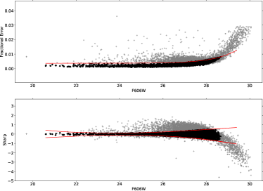
Figure 5: The distribution of the DAOPHOT sharp parameter (lower panel) and the fractional error (upper panel) versus the F606W magnitude for sources detected in the ACS/WFC data. The red lines in the lower panel enclose plus/minus three standard deviations from the mean value for the sharp obtained from the artificial star tests, estimated in magnitude bins of width 0.05 magnitudes. The red line in the upper panel indicates three standard deviations from the mean of the fractional error from the artificial star tests, calculated in the same magnitude bins. The sources plotted as black circles are those that pass all cleaning criteria in both of the F814W and F606W filters. The sources plotted as grey crosses were rejected by the cleaning cuts - they are too dissimilar from the ideal PSF statistics, as defined through the artificial star tests, to be identified as stars, by one or more of the criteria, even if they pass the requirements shown in this plot.

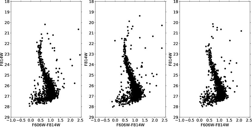
Figure 6: The cleaned DAOPHOT photometric data for each of the three ACS/WFC pointings. As in Figure 2, the number of sources retrieved per pointing is generally consistent with the surface density contours in Figure 1. Pointing one (left panel) has 927 sources. Pointing three (middle panel) is closest to the center of Boo I and has 1,167 sources. Pointing five (right panel) has 941 sources.

As noted, the artificial star tests also allowed for the determination of the completeness of the sample. First, stars with locations within problematic areas of the image, such as in masked regions or too close to the edges, were removed. Next, both the input and retrieved artificial stars were binned into 0.05 magnitude bins, spanning the input magnitude range. The ratio $N(\text{retrieved})/N(\text{input})$ for each magnitude bin then determined the completeness of the photometry, as shown in Figure 7. The data have a $50\%$ completeness limit of 27.4 for F814W and 28.2 for F606W (both on the Vega magnitude system) and this is the effective depth that we adopted for our further analysis. For comparison, the faint limit reported in F814W for the previous, shallower HST ACS/WFC data (Gennaro et al., 2018) is 27.5 STMAG, corresponding to $\sim 26.2$ in the Vega magnitude system. We checked our retrieval process by cross-matching our final catalog with that of Brown et al. (2014). We found a match, using a matching radius of $0.5\arcsec$, for $92\%$ of our catalog brighter than STMAG of 26, and for $82\%$ of our catalog down to the faint limit given in Gennaro et al. (2018).

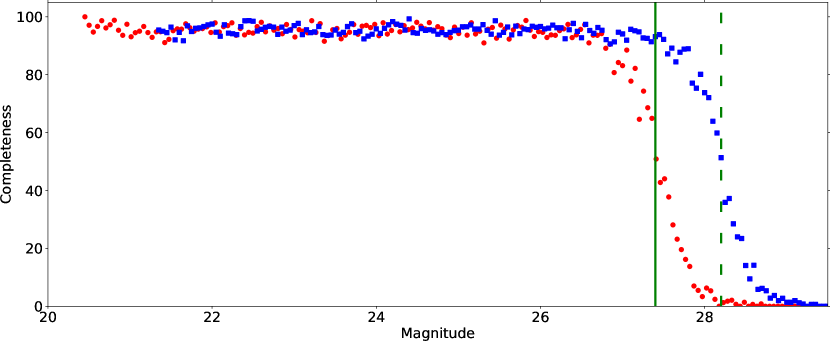
Figure 7: Completeness functions for the ACS/WFC observations, calculated from the artificial star tests as $N_{retrieved}/N_{added}$ in magnitude bin of width $0.05$, for F606W (blue squares) and F814W (red circles). The $50\%$ completeness magnitude for F606W is indicated by the vertical dashed green line at 28.2, and that for F814W by the vertical solid green line at 27.4.

4.6 Comparison between ePSF and DAOPHOT

We investigated the agreement between the ePSF and DAOPHOT photometry to determine the optimal catalog and photometry pipeline for the remainder of our analysis. The color magnitude diagram resulting from each pipeline are shown side-by-side in Figure 8. We matched the photometric catalog from each technique to compare the photometry, which required finding the shifts and scaling between the coordinate systems used in each analysis. The X and Y positions from ePSF are in the ACS/WFC detector coordinate system, while the X and Y positions from DAOPHOT are in the HST V2&V3 coordinate system (Ryon et al., 2019). There is an offset and rotation between these coordinate systems, as well as a plate-scale difference due to the pixel size resampling done in DrizzlePac. The offset, rotation, and scale were solved for by aligning stars brighter than a magnitude of 24 in each catalog for each pointing, and then the cleaned PSF DAOPHOT catalogs were matched to the ePSF catalogs.

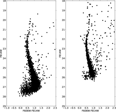
Figure 8: DAOPHOT photometry (left panel) and ePSF photometry (right panel), for all three pointings of the ACS/WFC observations. All sources consistent with being stellar are included. The metrics used to determine whether or not a detection is stellar differs between the two photometric catalogs, as discussed in the text.

We determined that a rotation of two degrees, a shift of $(\alpha,\delta)\sim(+9.7\arcsec,-8.6\arcsec)$, and a scaling factor of $\frac{5}{4}$ were needed to match the ePSF catalog to the DAOPHOT catalog. After the catalogues were matched, we found a mean magnitude offset of $\Delta m_{606}=-0.003$ and $\Delta m_{814}=-0.020$, where $\Delta m$ is the difference between the magnitudes from ePSF and DAOPHOT, shown graphically in Figure 9. The small, but non-zero, mean magnitude offset likely stems from the differing inputs into our photometry pipelines (i.e. single exposures versus drizzle-combined exposures). There is increased scatter at fainter magnitudes, as expected, and a slight skew towards more negative residuals at faint magnitudes, especially for F814W. The ePSF photometry reaches to $\sim 26.3$ in F814W, brighter than the DAOPHOT $50\%$ completeness limit, but still deeper than the previous dataset (from GO-12549), confirming that we achieved our goal of increased depth regardless of the choice of methodology of the photometry reduction. Blue straggler stars have previously been identified in Boo I as stars bluer and brighter than the dominant main-sequence turn-off (e.g. Belokurov et al., 2006b; Okamoto et al., 2012). We note that the final ePSF photometric catalog has a few more candidate blue straggler stars than does the DAOPHOT catalog. This difference is likely due to the differing cleaning processes - some of the DAOPHOT counterparts to the ePSF blue straggler candidates were rejected on the basis of their sharp statistics.

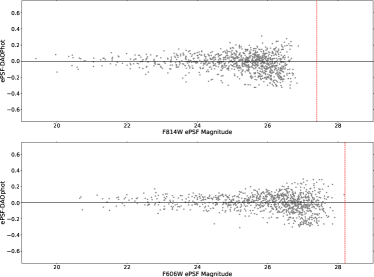
Figure 9: The magnitude residuals between ePSF and DAOPHOT photometry for the combined on-field ACS/WFC pointings, as a function of apparent magnitude from ePSF, for F814W (upper panel) and F606W (lower panel). The DAOPHOT 50% completeness level is shown as the vertical red dashed line, for context, and zero residual is indicated by the solid black line. There is excellent agreement at brighter magnitudes, with an increase in the residuals at fainter magnitudes, as expected.

The observed residuals depend on location on the image, which is plausibly related to the different levels of flexibility in the PSF fitting routines with ePSF and DAOPHOT. The two-dimensional map of the residuals in magnitudes between the two approaches is presented in Figure 10, where the non-linear variation across the ACS/WFC CCD chips is evident. This map was produced by fitting a second-order polynomial surface to the three-dimensional data of the X and Y positions of each match between the ePSF and DAOPHOT catalogues, and the residuals between the photometry. This spatial variation could be due to three factors: first, the PSF within ePSF is an empirical model derived from the data, whereas the PSF within DAOPHOT is an analytic Penny function which was fit to the data. Second, ePSF creates 45 empirical models across each ACS/WFC CCD chip and interpolates amongst the four nearest grid points for any arbitrary point in the ACS/WFC exposure, while within DAOPHOT, the PSF has fixed functional form and can vary across the chip up to quadratic order in the coordinates (Stetson, 1991). Third, the ePSF library is created for each calibrated ACS/WFC filter, while DAOPHOT uses the same base analytic function (a Penny function for the present discussed) and fits it to the data for each filter. The somewhat lower flexibility of DAOPHOT relative to ePSF results in a reduced ability to capture fully the spatial variation of the true PSF across the CCD chip (caused by variations in chip thickness, Anderson & King, 2006; Krist, 2003). The residuals can be either positive or negative for F606W, but are all negative for F814W. The all-negative values in the fit to the magnitude residuals for F814W, and the larger negative values in F606W, both come from the relatively higher number of detections with negative residuals at faint magnitudes, as seen in Figure 9. The amplitude of the residuals has a maximum value of $\sim 5\%$ at most, and reaches this extreme only in the very corners of the chip, for each filter, where sources were less likely to benefit from the dithering pattern. Thus while DAOPHOT may not perfectly model the variation of the PSF across the CCD chip, the average residual between the photometry derivations is low (less than 0.03 magnitudes), and DAOPHOT photometry reaches a fainter limit than does ePSF. We therefore adopt the DAOPHOT photometry catalog for the analysis of the low-mass stellar IMF (in paper II, Filion et al. in prep.)

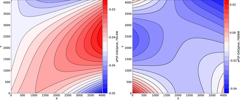
Figure 10: Two-dimensional maps of the residuals, in magnitudes, between the ePSF and DAOPHOT photometry for F814W (left panel) and F606W (right panel), for the ACS/WFC observations. The maximum amplitude of the residuals, corresponding to $\sim 5\%$, occurs towards the edges of the images. Typical residuals are $\simlt 3\%$.

4.7 Off-Field Observations

The off-field observations taken under our program (GO-15317) consist of one continuous exposure in each filter. As before, we used the bias corrected, flat-fielded and CTE-corrected data. We ran these off-field exposures through AstroDrizzle to correct for distortion (Kozhurina-Platais et al., 2015) and to produce output images of the same dimensions as the data for the on-field pointings. We then ran LACosmic (van Dokkum, 2001; McCully et al., 2018) to remove as many cosmic rays as possible, setting the threshold detection limit for cosmic rays to be four standard deviations above the background. A significant number of cosmic rays remained, however. DAOPHOT was then run on these cleaned exposures, following the same procedure as for the on-field data. Unfortunately, after inspection of the sources that were retrieved, we determined that the exposures remained too degraded by cosmic rays to be of use for our purposes and we proceeded with the analysis of data for an alternative off-field that we identified in the HST archive.

We searched the MAST archive for fields of similar Galactic latitude and longitude to those of Boo I (given in Table 1), with the further restrictions that the data have been taken in the same filters and with the same aperture (WFCENTER) as the on-field observations, and have similar exposure time to the original off-field data. We avoided fields with coordinates close to neighboring satellite galaxies such as Boo II or other known stellar over-densities, as the goal of the off-field data is to gain an understanding of the average Galactic contributions to the star counts in the Boo I fields. The observations that we selected are from GO-13393, in the line-of-sight with Galactic coordinates ($\ell,\,b{\rm)=(331^{\circ}.6,+46^{\circ}.7)}$, hereafter denoted by Off Field 2, and consist of four images per filter (see Table 2).

We combined the individual images with AstroDrizzle using the same parameters as the on-field ACS/WFC exposures. Photometry was done in DAOPHOT, again following the same procedure and conversions as for the on-field ACS/WFC exposures. Approximately 80 stars were retrieved in this field, the color-magnitude diagram for which is presented in Figure 15 alongside the color-magnitude diagram we obtained for Boo I  and predictions from the Besançon model of the Milky Way Galaxy at the appropriate coordinates. Note the higher number of Milky Way stars predicted for Off Field 2, reflecting its lower Galactic latitude. This field also has higher extinction than the line-of-sight towards Boo I and following the procedure from Section 4.4 we obtained $(A_{606},A_{814})=(0.148,0.096)$.

5 Photometry: WFC3/UVIS Data

The UVIS data were obtained in parallel mode, during the primary observations of fields in Boo I with ACS/WFC. WFC3/UVIS has a lower throughput than ACS/WFC (Dressel, 2019), and hence our observations with UVIS are not as deep our observations with ACS/WFC. These observations form the basis of our analysis of the star-formation history of Boo I (Paper III), where photometric precision for stars on the main sequence turn-off is crucial. We produced photometry for these fields using ePSF, as the high precision of ePSF photometry best fulfils these science goals.

The ePSF UVIS photometry procedure followed that for the ACS/WFC data, differing only in the values used for the photometric conversions. We adopted the appropriate Vega magnitude zero points for UVIS observations, and took the encircled energies from the UVIS website. The final ePSF color-magnitude diagram for each pointing is shown in Figure 11, where it may be noted that the limiting magnitude is not quite as faint as for the ACS/WFC photometry, as anticipated due to their different sensitivities. As before, only sources present in at least three exposures per filter are presented. The smaller pixel scale of UVIS compared to ACS/WFC has allowed for more precise photometry, which can be seen in the tighter main sequence and turnoff region of each pointing of Figure 11.

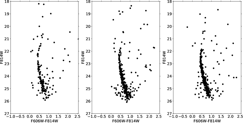
Figure 11: The color-magnitude diagram for each field of the UVIS data produced with ePSF. Only sources present in at least three exposures per filter are shown. Pointing A with 171 sources is leftmost, B with 309 sources is central, and C with 339 sources is rightmost.

6 Membership Selection

One of the more difficult aspects of photometric-only studies of the resolved stellar population of external galaxies is discerning which detections are likely members of the galaxy, and which are foreground/background contamination. To this end, the population(s) of the galaxy are usually represented by theoretical isochrones and stars rejected or accepted on the basis of proximity to the isochrone in the color-magnitude plane. Previous studies (e.g. Wyse et al., 2002; Belokurov et al., 2006b) simply defined a polygon encompassing a single isochrone, with properties matching those of the dominant population, and define all stars falling inside of the polygon as members, discarding those falling outside of the selected region. We developed a statistical method that builds on this approach and assigns a weight to each star based on its distance in color from a pair of isochrones, selected to bracket the known properties of Boo I, and that takes photometric errors into account. A high weight indicates a location on the color-magnitude diagram that is consistent with membership of Boo I and, conversely, a low weight indicates a non-member.

Roderick et al. (2015) devised a weighting scheme using Gaussian distributions in color space, centered on an isochrone representative of the mean population of the galaxy under study. We adopted a similar weighting scheme, but extended the technique through the use of two isochrones. As noted earlier, there is a significant metallicity spread in Boo I and this manifests itself through a broadening in color of the lower main sequence, below $\sim 0.5{\cal M_{\odot}}$, where sensitivity to metallicity is maintained, even at the low values relevant for Boo I. The goal of this work was to reach $\leq 0.3{\cal M_{\odot}}$ and thus it was especially important to devise a scheme that incorporated both the effect of the metallicity spread and the increasing photometric error at fainter magnitudes.

We selected isochrones from the Dartmouth Stellar Evolution Database (Dotter et al., 2008), as they allow fine-sampling of the low-mass regime of interest, plus they provide alpha-enhanced isochrones in the appropriate photometric bands for both ACS/WFC and WFC3/UVIS. We defined the most metal-poor and the most metal-rich isochrones to use by taking into account the trend of decreasing alpha-abundance enhancement with increasing iron abundances seen in Boo I member stars, noted above in Section 2. We adopted ${\rm[Fe/H]}=-3.5$, ${\rm[\alpha/Fe]=0.5}$ for the lowest metallicity, and ${\rm[Fe/H]}=-1.8$, ${\rm[\alpha/Fe]=0.1}$ for the highest metallicity. We obtained the appropriate metallicities (${\rm[M/H]}$) of the isochrones from the ${\rm[Fe/H]}$ and ${\rm[\alpha/Fe]}$ values using the transformation determined by Salaris et al. (1993) and refined by Salaris & Cassisi (2005):

$${\rm{\rm[M/H]}={\rm[Fe/H]}+\log(0.694\times 10^{[\alpha/Fe]}+0.306)}$$

This gave values of ${\rm[M/H]}=-3.1$ and ${\rm[M/H]}=-1.7$ for the lowest and highest metallicity isochrones to be used in defining the properties of Boo I stars in color-magnitude space. However, the most metal-poor isochrone that covers the required low-mass range that is provided by Dotter et al. (2008) has ${\rm[M/H]}=-2.5$ (isochrones of ${\rm[M/H]}=-2.688$ and ${\rm[M/H]}=-3.188$ are available, but lack entries for masses below $\sim 0.65{\cal M_{\odot}}$). Happily, the sensitivity of the color along the lower main sequence to metallicity is predicted to saturate below $\sim-2.5$ dex, with minimal difference between isochrones with ${\rm[M/H]}=-2.5$ and ${\rm[M/H]}=-3.0$ (A. Dotter, priv. comm.) In light of this, plus the advantages of this set of isochrones noted above, we adopted ${\rm[M/H]}=-2.5$ as the lowest metallicity isochrone, even though this is $\sim 0.5$ dex higher than the lowest published metallicity for a radial-velocity member of Boo I (Norris et al., 2010a). We adopted a fixed age of 13 Gyr and shifted the isochrones to apparent magnitudes and colors appropriate for an assumed distance of $62$ kpc and reddening and extinction from dust, as discussed in Section 4. A plot of these isochrones overlaid on the DAOPHOT ACS/WFC color-magnitude diagram for the Boo I fields is presented in Figure 12.

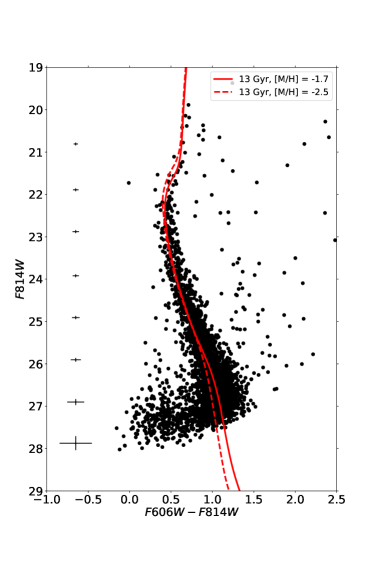
Figure 12: The cleaned DAOPHOT color-magnitude diagram for all three on-field ACS/WFC paintings combined. The solid red curve corresponds to a 13 Gyr, [M/H] = -1.7 isochrone, and the dashed curve a 13 Gyr, [M/H] = -2.5 isochrone, chosen to represent the observed range in metallicity in Boo I. Both isochrones have been corrected for dust and shifted to apparent magnitudes appropriate for an assumed distance of 62 kpc. The photometric error at fiducial magnitude levels, estimated following the discussion in Section 4.3, are indicated on the figure, at left. Note the divergence of the isochrones at lower masses, due to the increased sensitivity of the opacity to metallicity in this regime.

We investigated the identification of non-Boo I contaminants by first defining Gaussian distributions in color, centered on each of the two isochrones described above, and with mean and dispersion varying with the apparent magnitude along the isochrone. The mean of each distribution equaled the color of the dust-adjusted isochrone at that magnitude, while we set the dispersion to be three times the mean photometric error of the data within a bin of width 0.01 magnitudes, centered at that magnitude. We then defined the membership weight, $w_{i}$ for a given star of color $c_{i}$, F814W apparent magnitude $I_{i}$, with corresponding mean color error $\sigma_{i}$ as:

$$w_{i}=\frac{1}{2}\big{[}\exp{\frac{-(c_{i}-\mu_{1})^{2}}{2(3\sigma_{i})^{2}}}+\exp{\frac{-(c_{i}-\mu_{2})^{2}}{2(3\sigma_{i})^{2}}}\big{]},$$

where $\mu_{1}$ is the color of the ${\rm[M/H]=-1.7}$ isochrone at $I_{i}$, and $\mu_{2}$ is the color of the ${\rm[M/H]=-2.5}$ isochrone at $I_{i}$. Thus a star lying close to either of the isochrones will be assigned a weight close to unity while stars that lie far from either isochrone will be assigned a low weight. The most straightforward application is to identify non-members.

This technique can be thought of as defining membership by drawing a polygon around an isochrone, but where the width of the polygon at any apparent magnitude is set by the choice of threshold value for the weight, below which a star is rejected as a non-member. The fact that photometric errors are incorporated into the calculation of the weight provides for a widening at fainter magnitudes even for fixed threshold in the weight. The physical widening of the lower main sequence due to the sensitivity of the color of low-mass stars to metallicity is captured through the use of the two isochrones that represent the range in metallicity of stars in Boo I. This technique does not account for the shape of the metallicity distribution, however, which results in some stars lying between the isochrones receiving a weight less than unity.

The color-magnitude diagram color-coded by the weights calculated in this manner is shown in Figure 13. We cross-matched our catalog with spectroscopic studies of Boo I in the literature, to test our technique. We found four stars with matches, two radial-velocity Boo I member stars from Koposov et al. (2011) and one radial-velocity member plus one non-member from Martin et al. (2007). Our technique assigned a weight above $0.7$ to each of the radial-velocity members and a very low weight ($\sim 0$) to the non-member. These stars with spectroscopic information are indicated by special symbols in Figure 13. It is clear from the Figure that adopting a threshold weight of $\sim 0.5$ would separate stars occupying the locus of the main sequence and turn-off region from those that are more dispersed across the color-magnitude diagram.

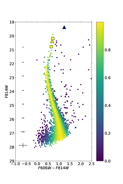
Figure 13: The cleaned DAOPHOT color-magnitude diagram of the on-field ACS/WFC data, as shown in Figure 14, now colored by weight, as indicated by the color bar at right. The high-weight stars (yellow) fall along the main sequence and turn-off region, while low-weight stars (blue) lie either to faint magnitudes with blue colors or redward of the main sequence. The yellow (high-weight) square symbols indicate radial-velocity member stars from Koposov et al. (2011) and the yellow triangle indicates a radial-velocity member from Martin et al. (2007). The navy (low-weight) triangle indicates a field star from Martin et al. (2007).

Thus far we have ignored the presence of binary systems, which would lie to the red of the single-star main sequence, and indeed Figure 13 shows a band of low-weight sources occupying that locus. We therefore defined ‘equal-mass binary isochrones’ by shifting the two isochrones brighter in apparent magnitude, subtracting 0.75 mag. We then re-calculated the weights based on position relative to these shifted isochrones. This procedure returned $108$ stellar sources, or $3.4\%$ of our full sample, which received a weight below 0.5 using the single-star isochrones but received a weight above this value using the ‘equal-mass binary’ isochrones. These sources are identified in Figure 14 and could be unresolved binary systems.

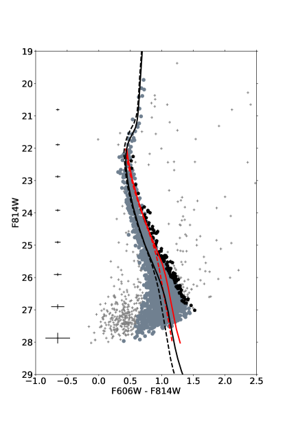
Figure 14: The cleaned, DAOPHOT color-magnitude diagram as in Figure 14 and Figure 13, now with different symbols to indicate weight and possible binarity. The solid black line indicates a 13 Gyr, $\rm[M/H]=-1.7$ isochrone, and the solid red line is this isochrone shifted brighter by 0.75 magnitudes, to mimic an equal-mass binary sequence. The dotted black line is a 13 Gyr, $\rm[M/H]=-2.5$ isochrone, and again the dotted red line is this isochrone shifted 0.75 magnitudes brighter. The grey filled circles represent stars that have weight greater than 0.5 based on distance from the unshifted isochrones, while the filled black pentagons, which occupy the locus of possible unresolved binaries, have weight greater than 0.5 based on the shifted isochrones, but below 0.5 on the unshifted isochrones. The grey crosses represent all other sources consistent with being stellar.

Assuming the $28\%$ binary fraction found for Boo I  in Gennaro et al. (2018), this translates to roughly $12\%$ of all binaries being rejected by cutting on a weight of $0.5$, if every one of the selected sources is an unresolved binary member of Boo I. Though relative to our total sample, the number of potentially rejected binaries is small, the likely possibility that this technique could reject true members of Boo I depending on the selected weight value motivates the more sophisticated Bayesian approach we adopt in Paper II.

As noted earlier, blue straggler stars should also be present within Boo I, but since these are plausibly evolved from close-binary systems they also will not be properly treated in any weighting scheme that was based on single-star stellar evolution models. The blue sources near the main sequence turn-off in the colour magnitude diagram may well be members of Boo I, but these candidate blue stragglers must be treated independently.

6.1 Non-Member Contamination

The two main sources of possible contamination in the lines-of-sight towards Boo I are background galaxies and foreground stars. The background galaxies should have been largely removed during the artificial-star tests and associated cleaning of the DAOPHOT photometry routines, due to their non-stellar PSF. However, faint, blue high-redshift galaxies are expected to be barely resolved even in HST images (Bedin et al., 2008) and will not be removed. Similarly, non-member stars will be included in the DAOPHOT catalog. We estimated the importance of these sources of contamination through both the predictions of theoretical models of the distribution of stars in the Milky Way and the analysis of photometry for an offset field with Galactic coordinates as well-matched as possible to those of Boo I.

6.1.1 Contamination by Milky Way Stars

We used the Besançon model (Robin et al., 2003) to make predictions for the contribution of stars in the Milky Way along the lines-of-sight of this study. We created simulated star counts for Off Field 2 and the Boo I fields. The Besançon model assumes smooth density laws for each of the main stellar components, namely stellar halo, bulge, thick disk and thin disk. Boo I lies in the ‘Field of Streams’ (Belokurov et al., 2006a) and several streams are close in projection and may contribute additional contamination beyond that predicted by the model. The Besançon model does not provide output in HST photometric bands and we selected the Johnsons-Cousins (V, I) system for the output. We then compared the predicted distribution of stars in the color-magnitude diagram to an isochrone representative of Boo I  in this photometric system, rather than attempt to convert between the magnitude systems.

At these faint magnitudes and intermediate latitudes, the expected contribution from the Milky Way should be predominantly lower main-sequence stars and white dwarfs from the thick disk and halo. The predicted distributions of the Milky Way stars in color-magnitude space are shown in the upper panels of Figure 15, and indeed the stars are mostly low-mass dwarfs from the halo and thick disk and the majority falls significantly redward of the isochrone representative of the mean population in Boo I. The predicted distribution shown in the upper righthand panel of Figure 15, in the line-of-sight towards Boo I, contains fewer than $\sim 30$ Milky Way stars which have colors and magnitudes overlapping with Boo I member stars. The remaining Milky Way contaminant stars, also $\sim 30$ in number, would be removed through an application of the membership weighting scheme described above. Foreground stars should have a higher proper motion than do members of Boo I and the cross-match with the earlier data from GO-12549 can be used to identify non-members, even those similar in color and magnitude to Boo I members. The time baseline from these first-epoch observations to our observations is 7 years, implying an expected shift in position for a star at distance $d$, with transverse velocity $v_{t}$, of amplitude $\sim 0.03\arcsec{\rm(}v_{t}/100{\rm km/s)}{\rm(5kpc}/d)$. Remembering that the drizzled images have a scale of $0.04\arcsec$/pixel, this shift should be detectable for many foreground stars.

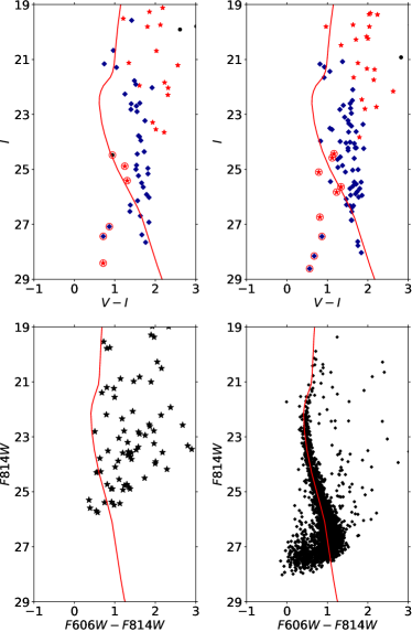
Figure 15: Upper panels: The predicted distributions of Milky Way stars in color-magnitude space from the Besançon model, for lines-of-sight corresponding to Off Field 2 (left) and Boo I (right). The output from the Besançon model is plotted in Johnsons-Cousins V and I. Halo stars are plotted as dark blue diamonds, thick-disk stars as red stars, and thin-disk stars as black circles. White dwarfs are indicated by a red circle around the symbol. Lower panels: Color-magnitude diagrams from the DAOPHOT photometry for Off Field 2 (left) and Boo I (right). The red curve in all panels is a 13 Gyr isochrone of metallicity equal to the peak of the observed metallicity distribution of Boo I, ${\rm[M/H]}=-2.2$, appropriately adjusted for dust in that line-of-sight and an assumed distance of 62 kpc.

The distribution of stellar sources in the off-field is shown in the lower left panel of Figure 15, with the predictions from the Besançon model in the upper left panel. The lower latitude of this field is reflected in the higher number of stars predicted, but again most sources lie far from the locus of the main population of Boo I. It should be noted that while the off-field data do not reach as faint as the Boo I field data, we use the off-field to understand the contribution of stars that are not members of Boo I. The majority of stellar contaminants are brighter than $\sim 25.5$ (as seen in Figure 15), and the cloud of blue sources around 27th magnitude are likely faint background galaxies and a few Galactic white dwarfs, discussed in Section 6.1.2. The relative importance of stellar contaminants is higher above a magnitude of $\sim 25.5$, motivating our use of a shallower off-field.

6.1.2 Faint Galaxy Contamination

The faint blue sources (colors $\simlt 0.5$, magnitudes $\simgt 26$) in the color-magnitude diagrams are likely to be predominantly high-redshift, marginally resolved galaxies, plus a few white dwarfs in the Milky Way (they are too bright to be white dwarfs in Boo I). The analysis by Bedin et al. (2008) supports the idea that there is a population of blue galaxies that is not distinguishable from stars in ACS/WFC images, using standard techniques. Those authors re-analyzed the data from the Hubble Ultra Deep Field (Beckwith et al., 2006), applied their stellar photometric pipeline and cleaning and found that faint blue galaxies made it through the processing and occupied a location on the color-magnitude diagram that is overlapping, but not identical to, the region that we see populated (see their Figure 9). Though we adopted a different photometric pipeline and cleaning process than did Bedin et al. (2008), it is likely that the faint, blue sources of our analysis are also faint galaxies. This idea is further supported by inspecting the sharp distribution of the faint blue detections, which one would expect to peak at positive values for unresolved galaxies (a wider PSF than a true stellar object). Indeed, in both F606W and F814W, the sharp distribution is peaked at positive values, but still small enough to have passed through the cleaning process ($\simlt 0.2$, versus $\sim$ 0 for the remaining sources in our catalog). Happily, the projected location of faint blue galaxies in color-magnitude space is bluer than low-mass stars of the metallicity and distance of Boo I, as evidenced by the isochrones in Figure 12 and by the discussion in Bedin et al. (2008). This separation in color-magnitude space leads us to conclude that these faint blue galaxies do not severely contaminate our sample. The bulk of these sources were given low weight (see Figure 13) and so would be removed by our membership scheme.

7 Discussion and Conclusions

The core goal of this work was to produce photometry for stars in Boo I, reaching as faint as possible down the main sequence, with $0.3{\cal M_{\odot}}$ being the target limiting mass. As discussed above, in Section 4.5, the ACS/WFC DAOPHOT photometry has a $50\%$ completeness limit of 27.4 Vega magnitude in F814W, and 28.2 Vega magnitude in F606W. These correspond to absolute magnitudes of +8.41 in F814W and +9.20 in F606W (using the distance modulus given in Table 1 and dust extinction from Section 4.4).

The Dotter et al. (2008) models we used in Section 6 translate the F814W limit to $0.29\cal M_{\odot}$ for $[M/H]=-1.7$ and $0.26\cal M_{\odot}$ for $[M/H]=-2.5$.Cassisi et al. (2000) calculated models for very low mass, low metallicity stars that we can use to obtain an independent estimate of the limiting mass. Their lowest metallicity models had $Z=0.0002$ and an age of 10 Gyr (see their Table 1). This age is younger than that usually derived for Boo I, but there should be negligible effect on the predicted luminosities of the low-mass stars of interest. These models provide a low-mass limit of between $0.3\cal M_{\odot}$ and $0.25\cal M_{\odot}$ for our F814W $50\%$ completeness limit. We therefore conclude that we did, indeed, produce photometry that reaches stars of $0.3\cal M_{\odot}$ or lower, achieving our goal.

This low-mass limit of $\simlt 0.3{\cal M_{\odot}}$ allows us to enter the regime discussed by El-Badry et al. (2017), where potential deviations from the Milky Way IMF can be discerned. The second paper in this series, Filion et al. (2021a.), uses the results of this paper in a Bayesian analysis (allowing unresolved binaries to be incorporated) of the low-mass end of the stellar IMF of Boo I. The high precision UVIS photometry will be employed in paper III Filion et al. (2021b.), alongside the ACS/WFC photometry, to constrain the star-formation history of Boo I. These future studies will be aided by proper motions derived from our observations and those of GO-12549, which will be used to identify non-member stars.

8 Acknowledgements

CF and RFGW are grateful for support through the generosity of Eric and Wendy Schmidt, by recommendation of the Schmidt Futures program. RFGW thanks her sister, Katherine Barber, for her support of this research. We thank Aaron Dotter for his help with the Dartmouth stellar evolution models. This research is based on observations made with the NASA/ESA Hubble Space Telescope obtained from the Space Telescope Science Institute, which is operated by the Association of Universities for Research in Astronomy, Inc., under NASA contract NAS 5–26555. These observations are associated with programs GO-15317, GO-12549, GO-13393. Support for this analysis of data from program 15317 was provided by NASA through a grant from the Space Telescope Science Institute, which is operated by the Association of Universities for Research in Astronomy, Inc., under NASA contract NAS 5–26555. This work has made use of the SVO Filter Profile Service http://svo2.cab.inta-csic.es/theory/fps/ supported from the Spanish MINECO through grant AYA2017-84089. This research has also made use of the VizieR catalogue access tool, CDS, Strasbourg, France (DOI : 10.26093/cds/vizier). The original description of the VizieR service was published in Ochsenbein et al. (2000). Additionally, this work made use of the SciServer science platform (www.sciserver.org). SciServer is a collaborative research environment for large-scale data-driven science. It is being developed at, and administered by, the Institute for Data Intensive Engineering and Science at Johns Hopkins University. SciServer is funded by the National Science Foundation through the Data Infrastructure Building Blocks program and others, as well as by the Alfred P. Sloan Foundation and the Gordon and Betty Moore Foundation.

HST (ACS, WFC3)

References

- Allard et al. (1997) Allard, F., Hauschildt, P. H., Alexander, D. R., et al. 1997, ARA&A, 35, 137
- Anderson & King (2000) Anderson, J., & King, I. R. 2000, PASP, 112, 1360
- Anderson & King (2006) Anderson, J., & King, I. R. 2006, Instrument Science Report ACS 2006-01
- Anderson et al. (2008a) Anderson, J., King, I. R., Richer, H. B., et al. 2008, AJ, 135, 2114
- Anderson et al. (2008b) Anderson, J., Sarajedini, A., Bedin, L. R., et al. 2008, AJ, 135, 2055
- Astropy Collaboration et al. (2013) Astropy Collaboration, Robitaille, T. P., Tollerud, E. J., et al. 2013, A&A, 558, A33
- Astropy Collaboration et al. (2018) Astropy Collaboration, Price-Whelan, A. M., Sipőcz, B. M., et al. 2018, AJ, 156, 123
- Avila et al. (2015) Avila, R. J., Hack, W., Cara, M., et al. 2015, in Astronomical Society of the Pacific Conference Series, Vol. 495, Astronomical Data Analysis Software and Systems XXIV (ADASS XXIV), ed. A. R. Taylor & E. Rosolowsky, 281
- Baraffe et al. (1997) Baraffe, I., Chabrier, G., Allard, F., et al. 1997, A&A, 327, 1054
- Bastian et al. (2010) Bastian, N., Covey, K. R., & Meyer, M. R. 2010, ARA&A, 48, 339
- Beckwith et al. (2006) Beckwith, S. V. W., Stiavelli, M., Koekemoer, A. M., et al. 2006, AJ, 132, 1729
- Bedin et al. (2008) Bedin, L. R., King, I. R., Anderson, J., et al. 2008, ApJ, 678, 1279
- Belokurov et al. (2006a) Belokurov, V., Zucker, D. B., Evans, N. W., et al. 2006a, ApJ, 642, L137
- Belokurov (2013) Belokurov, V. 2013, New A Rev., 57, 100
- Belokurov et al. (2006b) Belokurov, V., Zucker, D. B., Evans, N. W., et al. 2006b, ApJ, 647, L111
- Bohlin (2016) Bohlin, R. C. 2016, AJ, 152, 60
- Brown et al. (2014) Brown, T. M., Tumlinson, J., Geha, M., et al. 2014, ApJ, 796, 91
- Cassisi et al. (2000) Cassisi, S., Castellani, V., Ciarcelluti, P., et al. 2000, MNRAS, 315, 679
- Chabrier (2003) Chabrier, G. 2003, PASP, 115, 763
- Currie et al. (2014) Currie, M. J., Berry, D. S., Jenness, T., et al. 2014, in ASP conference series, Vol. 485, Astronomical Data Analysis Software and Systems XXIII, ed. N. Manset & P. Forshay, 391
- de los Reyes et al. (2020) de los Reyes, M. A. C., Kirby, E. N., Seitenzahl, I. R., et al. 2020, ApJ, 891, 85
- Dolphin (2016) Dolphin, A. 2016, DOLPHOT: Stellar photometry, ascl:1608.013
- Dotter et al. (2008) Dotter, A., Chaboyer, B., Jevremović, D., et al. 2008, ApJS, 178, 89
- Dressel (2019) Dressel, L. 2019, ”Wide Field Camera 3, HST Instrument Handbook,” Version 12 (Baltimore: STScI)
- El-Badry et al. (2017) El-Badry, K., Weisz, D. R., & Quataert, E. 2017, MNRAS, 468, 319
- Feltzing et al. (1999) Feltzing, S., Gilmore, G., & Wyse, R. F. G. 1999, ApJ, 516, L17
- Feltzing et al. (2009) Feltzing, S., Eriksson, K., Kleyna, J., et al. 2009, A&A, 508, L1
- Frebel et al. (2016) Frebel, A., Norris, J. E., Gilmore, G., et al. 2016, ApJ, 826, 110
- Gaia Collaboration et al. (2018) Gaia Collaboration, Helmi, A., van Leeuwen, F., et al. 2018, A&A, 616, A12
- Gennaro et al. (2018) Gennaro, M., Tchernyshyov, K., Brown, T. M., et al. 2018, ApJ, 855, 20
- Geha et al. (2013) Geha, M., Brown, T. M., Tumlinson, J., et al. 2013, ApJ, 771, 29
- Gilmore et al. (2013) Gilmore, G., Norris, J. E., Monaco, L., et al. 2013, ApJ, 763, 61
- Gonzaga & et al. (2012) Gonzaga, S., & et al. 2012, The DrizzlePac Handbook
- Grcevich & Putman (2009) Grcevich, J., & Putman, M. E. 2009, ApJ, 696, 385 (erratum 2016, ApJ, 824, 151)
- Grillmair et al. (1998) Grillmair, C. J., Mould, J. R., Holtzman, J. A., et al. 1998, AJ, 115, 144
- Hughes et al. (2014) Hughes, J., Wallerstein, G., Dotter, A., et al. 2014, MNRAS, 439, 788
- Hunter (2007) Hunter, J. D. 2007, Computing in Science & Engineering, 9, 90
- Ibata et al. (2019) Ibata, R. A., Malhan, K., & Martin, N. F. 2019, ApJ, 872, 152
- Ishigaki et al. (2014) Ishigaki, M. N., Aoki, W., Arimoto, N., et al. 2014, A&A, 562, A146
- Kalirai et al. (2013) Kalirai, J. S., Anderson, J., Dotter, A., et al. 2013, ApJ, 763, 110
- Koposov et al. (2011) Koposov, S. E., Gilmore, G., Walker, M. G., et al. 2011, ApJ, 736, 146
- Kozhurina-Platais et al. (2015) Kozhurina-Platais, V., Borncamp, D., Anderson, J., et al. 2015, Instrument Science Report ACS/WFC 2015-06
- Krist (2003) Krist, J. 2003, Instrument Science Report ACS 2003-06
- Kroupa (2001) Kroupa, P. 2001, MNRAS, 322, 231
- Kroupa (2002) Kroupa, P. 2002, Science, 295, 82
- Kroupa et al. (2013) Kroupa, P., Weidner, C., Pflamm-Altenburg, J., et al. 2013, in Planets, Stars and Stellar Systems. Volume 5: Galactic Structure and Stellar Populations, ed. T. D. Oswalt & G. Gilmore (Dordrecht: Springer), 115
- Lai et al. (2011) Lai, D. K., Lee, Y. S., Bolte, M., et al. 2011, ApJ, 738, 51
- Lauer (1999a) Lauer, T. R. 1999, PASP, 111, 227
- Lauer (1999b) Lauer, T. R. 1999, PASP, 111, 1434
- Martin et al. (2007) Martin, N. F., Ibata, R. A., Chapman, S. C., et al. 2007, MNRAS, 380, 281
- Martin et al. (2008) Martin, N. F., de Jong, J. T. A., & Rix, H.-W. 2008, ApJ, 684, 1075
- McCully et al. (2018) McCully, C., Crawford, S., Kovacs, G., et al. 2018, Astropy/Astroscrappy: V1.0.5 Zenodo Release, v1.0.5, Zenodo, doi:10.5281/zenodo.1482019
- McKinney (2010) McKinney, W. 2010, Proceedings of the 9th Python in Science Conference (SciPy,56) ed. S. van der Walt and J. Millman
- Muñoz et al. (2006) Muñoz, R. R., Carlin, J. L., Frinchaboy, P. M., et al. 2006, ApJ, 650, L51
- Muñoz et al. (2018a) Muñoz, R. R., Côté, P., Santana, F. A., et al. 2018, ApJ, 860, 66
- Muñoz et al. (2018b) Muñoz, R. R., Côté, P., Santana, F. A., et al. 2018, ApJ, 860, 65
- Newman et al. (2017) Newman, A. B., Smith, R. J., Conroy, C., et al. 2017, ApJ, 845, 157
- Norris et al. (2008) Norris, J. E., Gilmore, G., Wyse, R. F. G., et al. 2008, ApJ, 689, L113
- Norris et al. (2010a) Norris, J. E., Gilmore, G., Wyse, R. F. G., et al. 2010, ApJ, 722, L104
- Norris et al. (2010b) Norris, J. E., Wyse, R. F. G., Gilmore, G., et al. 2010, ApJ, 723, 1632
- Ochsenbein et al. (2000) Ochsenbein, F., Bauer, P., & Marcout, J. 2000, A&AS, 143, 23
- Okamoto et al. (2012) Okamoto, S., Arimoto, N., Yamada, Y., et al. 2012, ApJ, 744, 96
- Penny & Dickens (1986) Penny, A. J., & Dickens, R. J. 1986, MNRAS, 220, 845
- Robin et al. (2003) Robin, A. C., Reylé, C., Derrière, S., et al. 2003, A&A, 409, 523
- Roderick et al. (2015) Roderick, T. A., Jerjen, H., Mackey, A. D., et al. 2015, ApJ, 804, 134
- Roderick et al. (2016) Roderick, T. A., Mackey, A. D., Jerjen, H., et al. 2016, MNRAS, 461, 3702
- Ryon et al. (2019) Ryon, J. E., et al. 2019, “ACS Instrument Handbook,” Version 18.0 (Baltimore: STScI)
- Salaris & Cassisi (2005) Salaris, M., & Cassisi, S. 2005, Evolution of Stars and Stellar Populations (New York: Wiley)
- Salaris et al. (1993) Salaris, M., Chieffi, A., & Straniero, O. 1993, ApJ, 414, 580
- Salpeter (1955) Salpeter, E. E. 1955, ApJ, 121, 161
- Schechter et al. (1993) Schechter, P. L., Mateo, M., & Saha, A. 1993, PASP, 105, 1342
- Schlafly & Finkbeiner (2011) Schlafly, E. F., & Finkbeiner, D. P. 2011, ApJ, 737, 103
- Scoville et al. (2007) Scoville, N., Abraham, R. G., Aussel, H., et al. 2007, ApJS, 172, 38
- Siegel (2006) Siegel, M. H. 2006, ApJ, 649, L83
- Simon (2018) Simon, J. D. 2018, ApJ, 863, 89
- Simon (2019) Simon, J. D. 2019, ARA&A, 57, 375
- Sirianni et al. (2005) Sirianni, M., Jee, M. J., Benítez, N., et al. 2005, PASP, 117, 1049
- Smecker & Wyse (1991) Smecker, T. A., & Wyse, R. F. G. 1991, ApJ, 372, 448
- Sollima (2019) Sollima, A. 2019, MNRAS, 489, 2377
- Stetson (1987) Stetson, P. B. 1987, PASP, 99, 191
- Stetson (1991) Stetson, P. B. 1991, in proc. 3rd ESO/ST-EFC Data Analysis Workshop, eds P.J. Grosbøl & R.H. Warmels. ESO Conference and Workshop Proceedings, No. 38. (Garching: European Southern Observatory) p. 187
- STScI Development Team (2012) STScI Development Team 2012, DrizzlePac: HST image software, ascl:1212.011
- Taylor (2005) Taylor, M. B. 2005, in Shopbell P., Britton M., Ebert R., eds, Astronomical Society of the Pacific Conference Series Vol. 347, Astronomical Data Analysis Software and Systems XIV., p. 29
- Tody (1986) Tody, D. 1986, Proc. SPIE, 733
- Tody (1993) Tody, D. 1993, Astronomical Data Analysis Software and Systems II, 173
- VanderPlas et al. (2012) VanderPlas, J., Connolly, A. J., Ivezic, Z., et al. 2012, in Proceedings of Conference on Intelligent Data Understanding (CIDU), ed. K. Das, N. V. Chawla, & A. N. Srivastava (Los Alamitos, CA: IEEE), 47
- van Dokkum (2001) van Dokkum, P. G. 2001, PASP, 113, 1420
- Wyse (1998) Wyse, R. F. G. 1998, in The Stellar Initial Mass Function, ASP Conf Proc vol 142, eds G. Gilmore & D. Howell (ASP, San Francisco) p89
- Wyse & Gilmore (1992) Wyse, R. F. G., & Gilmore, G. 1992, AJ, 104, 144
- Wyse et al. (2002) Wyse, R. F. G., Gilmore, G., Houdashelt, M. L., et al. 2002, New A, 7, 395