Nonequilibrium Green’s functions for functional connectivity in the brain

Abstract

A theoretical framework describing the set of interactions between neurons in the brain, or functional connectivity, should include dynamical functions representing the propagation of signal from one neuron to another. Green’s functions and response functions are natural candidates for this but, while they are conceptually very useful, they are usually defined only for linear time-translationally invariant systems. The brain, instead, behaves nonlinearly and in a time-dependent way. Here, we use nonequilibrium Green’s functions to describe the time-dependent functional connectivity of a continuous-variable network of neurons. We show how the connectivity is related to the measurable response functions, and provide two illustrative examples via numerical calculations, inspired from C. elegans.

Understanding how neurons interact is fundamental to describing how their collective activity generates the complex dynamics of the brain. Advances in optogenetics and neuroimaging now allow activity to be stimulated in one neuron while simultaneously measuring the response of many others in a network Rickgauer2014 ; Emiliani2015 ; Yang2018 , providing insights into how signals travel through the brain. Functional connectivity encompasses the collection of strengths, signs, and time-varying properties that govern how a change in activity of one neuron affects another. Measuring functional connectivity would constrain simulations by providing a missing link between the anatomical connectivity and the neural dynamics. Further, measuring how functional connectivity changes can reveal what dynamical properties of the brain change with learning.

Most existing models of continuous-variable neural activity are formulated as differential equations ErmentroutBook2010 ; DayanAbbotBook2001 ; Wicks1996 ; Kunert2014 ; Kunert2017a ; Kunert2017b . These equations include parameters for local properties of direct connections in the network, such as the strengths of the synapses between two neurons. But those local properties cannot be measured directly in the network. Instead, experiments see an effective interaction between the two neurons, which includes contributions from indirect paths as well as the direct path.

An integral formulation, such as Brinkman2018 , is a more convenient formalism for transitioning between local direct connections and the effective ones that are more experimentally accessible. In the linear and time-translationally invariant (TTI) case (a condition that we will relax in this paper), the activity $\psi_{i}$ of neuron $i$ is

$$\psi_{i}(t)=\psi_{i,\mathrm{eq}}+\sum_{j\in\mathrm{all}}g_{0,ij}*\Delta\psi_{j}\,(t)+g_{0,i}^{\mathrm{ext}}*I^{\mathrm{ext}}_{i}(t),$$ (1)

where $\psi_{\mathrm{eq}}$ are the equilibrium activities of the neurons (which depend on the rest of the network) and $\Delta\psi$ the deviations from those values. $*$ denotes a convolution, $g_{0,ij}$ is the (TTI) Green’s function, or transfer function, describing the direct interaction $i\leftarrow j$ from neuron $j$ to neuron $i$. $g_{0,i}^{\mathrm{ext}}*I^{\mathrm{ext}}_{i}(t)$ denotes the effect of external perturbations.

Eq. (1) considers only direct paths between neurons. However, in a network $i$ and $j$ are connected by both direct and indirect paths, and one would have to solve Eq. (1) for each neuron and each time-step. If we know $\Delta\psi_{j}$ footnotem1 and want to calculate $\Delta\psi_{i}$, in a linear system we can condense the effect of the whole network in a single connected Green’s function $G^{j}_{0,ij}$ (the resolvent kernel in Volterra integral equations Linz1985 ), such that $\psi_{i}(t)=\psi_{i,\mathrm{eq}}+(G^{j}_{0,ij}*\Delta\psi_{j})(t)$. $G^{j}_{0,ij}$ is a solution to

$$G^{j}_{0,ij}=g_{0,ij}+\sum_{\mu\neq j}g_{0,i\mu}*G^{j}_{0,\mu j},$$ (2)

which is obtained recursively inserting the contributions of all the neurons in Eq. (1) (upper case is for connected, subscript 0 for linear and TTI, superscript $j$ means that $j$ is excluded from the sums. For when $\Delta\psi_{j}$ is sufficient and for the derivation, see the Supplement Supplement ). To probe the system, we can induce a perturbation $\delta\psi_{j}$ on top of the current state of the system $\bm{\psi=\psi_{\mathrm{eq}}+\Delta\psi}$ and obtain the connected response function $F_{0,ij}$ by measuring the produced $\delta\psi_{i}=F_{0,ij}*\delta\psi_{j}$. In the linear and TTI case, $F_{0,ij}=G^{j}_{0,ij}$.

One reason Green’s functions have found only limited use in neuroscience DayanAbbotBook2001 ; Brinkman2018 is that Green’s functions are usually defined only for linear and TTI systems, while the brain is highly nonlinear. Nonlinearities allow the brain to perform nontrivial computations and to have responses that depend on past history or sensory context. Nonlinear corrections to a Green’s function-like formulation via systematic expansion has previously been used to describe the effect of hidden neurons Brinkman2018 and spike train statistics Ocker2017 . Because the concept of a response function is intuitive, and an experiment can always be designed to measure a response function, it is worth working with expanded, or corrected, Green’s functions.

In this work we use nonequilibrium Green’s functions $G_{ij}$ NEDMFT ; Ocker2017 ; HerreraDelgado2020 to describe the time-dependent functional connectivity of a continuous-variable network of neurons, and discuss their relation to the nonequilibrium response functions $F_{ij}$ measured in experiments (absence of subscript 0 means nonequilibrium). While they retain the benefits of transfer functions, their nonequilibrium definition as a function of relative and absolute time makes them well-suited to capture nonlinearities and time-dependence in the brain, for example when synapses saturate, when synaptic adaptation occurs, or when neuromodulators change the cellular properties of the neurons in a time-dependent way. Nonequilibrium Green’s functions are used in other fields, like the theory of many-body systems in condensed matter physics, where they guide both theory and experiments NEDMFT . Note that here equilibrium refers to the time-invariance of the Green’s functions, not the neural activities.

We first present a general model-independent equation for the connected nonequilibrium response functions $F_{ij}$ (Eq. (5)), that allow us to write $\delta\psi_{i}(t)=F_{ij}*\delta\psi_{j}=\int dt_{1}\,F_{ij}(t,t_{1})\delta\psi_{j}(t_{1})$, and are obtained assuming sparse nonlinear connections, or edges, $(\alpha,\beta)$. These edges are described with nonequilibrium Green’s functions $g_{{\alpha\beta}}[\bm{\psi}]$ so that, formally, $\Delta\psi_{\alpha}=g_{{\alpha\beta}}[\bm{\psi}]*\Delta\psi_{\beta}=\int dt_{1}\,g_{{\alpha\beta}}[\bm{\psi}](t,t_{1})\Delta\psi_{j}(t_{1})$ for an isolated pair of neurons. Because $g_{{\alpha\beta}}[\bm{\psi}]$ is functionally dependent on the state $\bm{\psi}$ of the system it has to be calculated according to its nonlinear expression. Once it is calculated, however, other properties of the network, like the other Green’s functions and the response functions, are easily derived and computed.

We will describe how the $F_{ij}$s relate functional connectivity to experiments, apply this formalism to the nervous system of the nematode worm Caenorhabditis elegans, and illustrate the general theoretical results with numerical calculations.

Nonequilibrium response functions

As we derive an equation for the nonequilibrium response function $F_{ij}$, we will also address a seemingly puzzling experimental observation about the C. elegans nervous system. Characterizations of some synpases in the worm have shown that they are linear throughout a large part of the physiological range of membrane potentials Liu2009 ; Lindsay2011 ; Narayan2011 . However, we know that nonlinearities and time-dependence are critically important in the C. elegans nervous system and in nervous systems generally, because they allow the network to perform computations, including for example responding to sensory stimuli in a context dependent manner Mochi2019 ; Dobosiewicz2019 . How does a network have many linear edges but also show widespread nonlinear behaviors? In the integral formulation with nonequilibrium Green’s functions it is straightforward to show how these two observations can coexist.

We start by considering a network in which only one of the edges, $(\alpha,\beta)$, displays a significant nonlinearity. This is in contrast to an approach in Ocker2017 which assumes nonlinearities that are homogeneous over the network and then proceeds with their systematic expansion. We will show how a time-dependent change of a single edge, due e.g. to a nonlinearity, can change effective connections and response functions elsewhere in the network.

The direct Green’s function $g_{\alpha\beta}(t,t^{\prime})=g_{0,{\alpha\beta}}(t-t^{\prime})+\pi_{\alpha\beta}[\bm{\psi}](t,t^{\prime})$ for the nonlinear or time-dependent edge can be written as the sum of a linear and TTI term $g_{0,{\alpha\beta}}$ and a nonequilibrium term $\pi[\bm{\psi}]$, which depends on the state $\bm{\psi}$ of the system. For the isolated pair $\alpha\leftarrow\beta$, $g_{\alpha\beta}$ allows one to calculate the response function $f_{\alpha\beta}$ that determines $\delta\psi_{\alpha}$ measured in an experiment after a perturbation $\delta\psi_{\beta}$ on top of the current state $\bm{\psi=\psi_{\mathrm{eq}}+\Delta\psi}$. With $f_{\alpha\beta}$, one can write $\delta\psi_{\alpha}=f_{\alpha\beta}*\delta\psi_{\alpha}=\int dt_{1}\,f_{\alpha\beta}(t,t_{1})\delta\psi_{\beta}(t_{1})$, where nonlinearities and time-dependence are implicitly taken into account in the nonequilibrium $f_{\alpha\beta}$,

$$f_{\alpha\beta}(t,t^{\prime}) =g_{0,{\alpha\beta}}(t-t^{\prime})+\bar{\chi}_{\alpha\beta}[\bm{\psi}](t,t^{\prime}),$$ (3)

$$\bar{\chi}_{\alpha\beta}[\bm{\psi}](t,t^{\prime}) =\pi_{\alpha\beta}(t,t^{\prime})+\biggl{(}\frac{\delta\pi_{\alpha\beta}(t,t_{1})}{\delta\psi_{\beta}(t^{\prime})}*\psi_{\beta}(t_{1})\biggr{)}(t,t^{\prime}).$$ (4)

(see Supplemental material Supplement for more details)

The connected nonequilibrium response function $F_{ij}$ of a general effective edge $(i,j)$ in a network is obtained following similar steps to the ones leading to Eq. (2), but using Eq. (3) for the edge $(\alpha,\beta)$, and is

$$F_{ij}(t,t^{\prime})=F_{0,ij}(t-t^{\prime})+\big{(}F^{j}_{0,i\alpha}*\bar{\chi}_{\alpha\beta}*F_{\beta j}\big{)}(t,t^{\prime}),$$ (5)

where $(A*B)(t,t^{\prime})=\int dt_{1}\,A(t,t_{1})B(t_{1},t^{\prime})$. The response $\delta\psi_{i}$ to a perturbation $\delta\psi_{j}$ can be written as a simple convolution $\delta\psi_{i}(t)=(F_{ij}*\delta\psi_{j})(t)$ where $F_{ij}$ evolves due to the nonequilibrium terms $\bar{\chi}[\bm{\psi}]$ (and $\pi[\bm{\psi}]$). The $\pi[\bm{\psi}]$ and $\bar{\chi}[\bm{\psi}]$ we will consider below can be derived exactly, but there is no one recipe for calculating all possible $\pi[\bm{\psi}]$ and $\bar{\chi}[\bm{\psi}]$. Condensed matter physics provides useful approximations and techniques for calculating them in more complicated cases NEDMFT . We use the notation $F_{0}$ instead of $G_{0}$ to emphasize that we are discussing a response function. Eq. (5) contains different terms (see Supplemental material Supplement ) when $i$ and/or $j$ are equal to $\alpha$ and $\beta$.

The more the neurons on the edge $(\alpha,\beta)$ act as hubs in the network, the larger the fraction of the functional connectivity is affected by their nonlinearity. For example, $\beta$ could be an interneuron integrating inputs from multiple neurons. Sensory neurons can also act as hubs. Increasing evidence shows that, in C. elegans, sensory neurons are well interconnected with the rest of the network Dobosiewicz2019 . The application of a sensory stimulus could drive $(\alpha,\beta)$ in a nonlinear regime and, therefore, alter effective interactions between other neurons. The existence of many types of hubs in neural networks make the framework presented here particularly valuable.

Eqs. (3) and (5) describe an approximately linear regime on top of an arbitrary state of the system. Switching linear dynamical systems (SLDS) models Linderman2019 ; Costa2019 assume that such locally linear regimes exist. They describe the dynamics of a nonlinear system as a temporal sequence of linear systems each with different parameters, and have previously been applied to C. elegans. In existing SLDS models, the time-dependent switching between parameters is entirely phenomenological. In our approach, Eqs. (3), (5), and supplementary Eq.(14) Supplement , explicitly govern how nonlinearities in the network produce time-dependent changes to a linear system. Here the response functions contain the time-dependent parameters of the SLDS.

This framework has both computational and conceptual advantages. Once the nonlinear $\pi_{\alpha\beta}[\bm{\psi}]$ is calculated, the $F_{ij}$ can be calculated for a given effective edge $(i,j)$ via simple convolutions and without needing all the details of the network. In fact, it is only necessary to run the calculation for two effective edges: the selected edge $(i,j)$ and $(\beta,j)$. If the network has significant nonlinearities on multiple edges, the approach can still be used to calculate response functions, except now the last term in Eq. (5) becomes a summation running over all the nonlinear edges $(\alpha,\beta)$, and therefore the nonlinear calculation becomes more computationally intensive.

Experimental characterization

Importantly, $F_{ij}$ are the response functions that can be obtained in experiments on networks of neuron as responses to impulsive perturbations. The $F_{ij}$s are always well defined experimentally and theoretically, whether one is studying a complete or subsampled network (see the Experimental characterization section in the Supplemental Supplement ).

The local $f_{ij}$ are also of interest, however, because they are directly related to the anatomical connections between the neurons and to the molecular mechanisms responsible for the interactions between them. For models that use equations in differential form, several approaches have been proposed to fit local parameters from spontaneous neural activity, especially in spiking neurons Pillow2007 ; Soudry2015 ; Dunn2007 ; Tyrcha2014 ; Bravi2017 .

In the integral formulation, to obtain the local $f_{ij}$ from the measured $F_{ij}$, one can use deconvolutions and equations (2) and (5) under the condition of having a complete measurement of $F_{ij}$ for each pair $(i,j)$ and a suitable “scan” across the nonlinearities. While this is experimentally impractical for larger animals, it might be achievable soon on smaller ones like C. elegans. However, (de)convolutions are particularly susceptible to noise, so that the response functions might need to be parametrized depending on the level of noise. The ability to selectively introduce nonlinearities and the availability of fast routines to calculate the response functions will prove very valuable in fits, where functions have to be evaluated several times. We leave to future work the details of obtaining $f_{ij}$ from $F_{ij}$.

C. elegans nervous system

To do calculations, we need to provide explicit expressions for the equilibrium Green’s function and the nonlinear term $\pi$, beyond Eq. (5). We consider the equations used in Wicks1996 ; Kunert2014 to simulate neural dynamics in C. elegans. Here, the neural activity $\psi_{i}$ is the membrane potential $V_{i}$, and each neuron $i$ is described as a single electrical compartment Wicks1996 ; Kunert2014 via the equation

$$\partial_{t}V_{i}=-\gamma_{i}(V_{i}-E_{c,i})-\gamma_{ij}^{\mathrm{g}}(V_{i}-V_{j})-\gamma_{ij}^{\mathrm{s}}s_{ij}(V_{i}-E_{ij}),$$ (6)

where the constants $\gamma$ have dimensions of a conductance over a capacitance and describe leakage ($\gamma_{i}$); electrical synapses, or gap junctions ($\gamma_{ij}^{\mathrm{g}}$); and chemical synapses ($\gamma_{ij}^{\mathrm{s}}$). $E_{c,i}$ is the reversal potential of the leaking channels, and $E_{ij}$ the reversal potential of the ionotropic receptors at the synapse. $s_{ij}$ is a synaptic activity variable that evolves according to

$$\partial_{t}s_{ij}=a_{r}\phi_{ij}(V_{j})(1-s_{ij})-a_{d}s_{ij}.$$ (7)

$\phi_{ij}(V_{j})$ describes the dependence of the calcium influx in the presynaptic site on the presynaptic voltage, which triggers the release of vesicles into the synaptic cleft, and is modeled as $\phi_{ij}(V_{j})=1/\big{(}1+e^{-\beta_{ij}(V_{j}-V_{\mathrm{th},ij})}\big{)}$ Wicks1996 ; Kunert2014 . External stimuli in the form of currents $I_{\mathrm{ext},i}$ injected in neurons are added to Eq. (6) as $-I_{\mathrm{ext},i}/C_{i}$, where $C_{i}$ is the membrane capacitance of neuron $i.$

We obtain expressions for the equilibrium Green’s function of the system by linearizing Eqs. (6) and (7) around the equilibrium of the membrane potentials. With $\Delta V_{j}$ and $\Delta s_{ij}$ being the deviations from equilibrium, we obtain $\Delta V_{i}(t)=\big{(}g_{0,ij}^{\mathrm{g}}*\Delta V_{j}\big{)}(t)+\big{(}g_{0,ij}^{\mathrm{s}}*\Delta s_{ij}\big{)}(t)$ and $\Delta s_{ij}(t)=\big{(}\sigma_{0,ij}*\Delta V_{j}\big{)}(t)$. The total direct Green’s function ($V_{i}\leftarrow V_{j}$) is $g_{0,ij}=g_{0,ij}^{\mathrm{g}}+g_{0,ij}^{\mathrm{s}}*\sigma_{0,ij}$, with $\Delta V_{i}(t)=\big{(}g_{0,ij}*\Delta V_{j})(t)$. (Lower case means direct. See Supplement Supplement for the full expression.)

There are three sources of nonlinearities that can be added back: the saturation of the postsynaptic current when the postsynaptic membrane potential approaches the reversal potential of the ionotropic receptor through which the current flows (Eq. (6)); the saturation of the synaptic activity (which can range between $0$ and $1$) due to the finite number of receptors; and the sigmoidal dependence $\phi(V_{j})$ of the vescicle release on the presynaptic potential (Eq. (7)).

We obtain the full expression for the nonequilibrium $\sigma_{ij}[\bm{V}](t,t^{\prime})$, the Green’s function bringing from $V_{j}(t)$ to $s_{ij}(t)$, reinserting the nonlinear terms in the equations,

$$\sigma_{ij}(t,t^{\prime})=\frac{\sigma_{0,ij}(t-t^{\prime})}{\partial_{V_{j}}\phi\big{|}_{\mathrm{eq}}}\frac{\Delta\phi\big{(}V_{j}(t^{\prime})\big{)}}{\Delta V_{j}(t^{\prime})}\biggl{(}1-\frac{(\sigma_{ij}*\Delta V_{j})(t^{\prime})}{1-s_{ij,\mathrm{eq}}}\biggr{)}.$$ (8)

The nonequilibrium $g_{ij}[\bm{V}](t,t^{\prime})$ is

$$g_{ij}(t,t^{\prime})=g_{0,ij}^{\mathrm{g}}(t-t^{\prime})+g^{\mathrm{s}}_{0,ij}*\biggl{(}\bigg{(}1-\frac{\Delta V_{i}}{V_{i,\mathrm{eq}}-E_{ij}}\bigg{)}\sigma_{ij}\biggr{)}(t,t^{\prime}).$$ (9)

In the following examples, we will only consider the nonlinear contribution coming from $\sigma_{\alpha\beta}(t,t^{\prime})$, while we will keep the equilibrium $g_{0,{\alpha\beta}}(t-t^{\prime})$. The nonequilibrium response function $\chi$ defined by $\delta s_{\alpha\beta}(t)=\chi_{\alpha\beta}(t,t^{\prime})*\delta V_{\beta}(t)$, with $\delta V_{\beta}$ on top of the current state $V_{\beta,\mathrm{eq}}+\Delta V_{\beta}$, is given by

$$\begin{split}\chi_{\alpha\beta}&(t,t^{\prime})=\frac{\sigma_{0,{\alpha\beta}}(t-t^{\prime})}{\partial_{V_{\beta}}\phi\big{|}_{\mathrm{eq}}}\partial_{V_{\beta}}\phi\big{|}_{t^{\prime}}\bigg{(}1-\frac{(\sigma_{\alpha\beta}*\Delta V_{\beta})(t^{\prime})}{1-s_{{\alpha\beta},\mathrm{eq}}}\bigg{)}\\ &-\int_{t^{\prime}}^{t}dq\frac{\sigma_{0,{\alpha\beta}}(t-q)}{\partial_{V_{\beta}}\phi\big{|}_{\mathrm{eq}}(1-s_{{\alpha\beta},\mathrm{eq}})}\Delta\phi(\Delta V_{\beta}(q))\chi_{\alpha\beta}(q,t^{\prime}),\end{split}$$ (10)

with the direct response function $f_{\alpha\beta}=g^{\mathrm{s}}_{0,{\alpha\beta}}*\chi_{\alpha\beta}$.

Illustrative examples

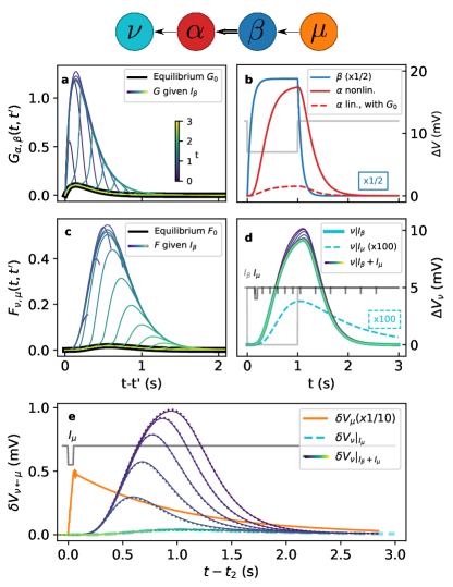
Figure 1: top Scheme of the network. a Nonequilibrium and equilibrium $G_{(0,)\alpha,\beta}(t,t^{\prime})$ for selected times $t$ (colored and black curves, respectively). b $\Delta V_{\beta}(t)$ (blue), and $\Delta V_{\alpha}(t)$ obtained with $G_{\alpha\beta}$ (solid red) and with $G_{0,{\alpha\beta}}$ (dashed red). The gray curve is $I_{\beta}$, with a baseline of $0$ and a peak of $-0.5$ pA (axis not shown). c Nonequilibrium and equilibrium $F_{(0,)\nu,\mu}(t,t^{\prime})$ for selected times $t$ (colored and black curves, respectively). Colors as in a. d $\Delta V_{\nu}$ obtained with stimulations $I_{\beta}$ (solid cyan), $I_{\mu}$ (dashed cyan, x100), and $I_{\beta}$ + $I_{\mu}$ (thin lines, colors as in a). Gray curve as in panel b. Black curve: current $I_{\mu}$, with a baseline of $0$ and a peak of $-0.1$ pA. Black ticks: times $t_{2}$ at which $I_{\mu}$ is injected. e $\delta V_{\nu\leftarrow\mu}$ induced by $I_{\mu}$ on top of the nonequilibrium state, calculated as $F_{\nu\mu}*\delta V_{\mu}\big{|}_{I_{\mu}}$ (dotted lines) and as $\Delta V_{\nu}\big{|}_{I_{\beta}+I_{\mu}}-\Delta V_{\nu}\big{|}_{I_{\beta}}$ (solid lines), for different times $t_{2}$ (colors as in a, $t_{2}$ as the black ticks in d). $\Delta V_{\nu}\big{|}_{I_{\mu}}$ (cyan dashed line, as in panel d). $\delta V_{\mu}|_{I_{\mu}}$ (orange line, x1/10) as produced by perturbation $I_{\mu}$ (black line) .

We provide numerical examples in two simple networks so that results can be understood intuitively. In the first example, we show how $F(t,t^{\prime})$ correctly captures the responses of the neurons to arbitrary stimulations. The example describes a form of gating in a simple feed-forward network with excitatory synaptic connections $\nu\leftarrow\alpha\Leftarrow\beta\leftarrow\mu$, where $\alpha\Leftarrow\beta$ is the only edge where we consider a nonlinearity (as depicted at the top of Fig. 1). We choose parameter values similar to those in Ref. Kunert2014 (see Supplement Supplement for more details). The main difference is that $V_{\mathrm{th},\alpha\beta}$ is set to $-10\,\mathrm{mV}$ Juusola1996 so that the resting potential of neuron $\beta$ sits at the bottom of the sigmoid $\phi_{\alpha\beta}(V_{\beta})$. Therefore, small perturbations around the resting potentials of neurons upstream of the nonlinear edge $(\alpha,\beta)$ produce only small responses downstream of that edge, as shown in Figure 1a and c, where the black curves show the equilibrium $G_{0,\alpha\beta}$ and $F_{0,\nu\mu}$ ($=G_{0,\nu\mu}$), respectively.

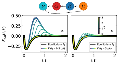
Figure 2: Nonequilibrium and equilibrium $F_{(0,)\nu,\mu}(t,t^{\prime})$ for selected times (colored and black curves, respectively), for currents into $\beta$ of 0.5 pA (a) and 3 pA (b). Scheme of the network (top).

The situation is different if there is a significant change of $V_{\beta}$, as could happen, for example, due to the application of an odor sensory stimulus. To simulate this, we inject a $0.5\,\mathrm{pA}$ external current $I_{\beta}$ into $\beta$ for $1$ s (gray curve in Fig. 1b), which induces a $\Delta V_{\beta}$ as shown in Fig. 1b (blue curve). As a consequence, $\phi_{\alpha,\beta}$ increases significantly and makes $G_{\alpha\beta}$ transiently larger than $G_{0,\alpha\beta}$, as shown in Fig. 1a for selected times $t$. A larger $G_{\alpha\beta}$ allows the activity in $\beta$ to reach $\alpha$ more efficiently (Fig. 1b solid red curve), compared to $G_{0,\alpha\beta}$ (Fig. 1b dashed red curve), and consequently also other neurons downstream of the edge $(\alpha,\beta)$.

In the time interval in which $G_{\alpha\beta}$ is enhanced, any other small perturbations upstream of the nonlinear edge can propagate more effectively to nodes downstream of the edge, compared to at equilibrium. For example, the response function $F_{\mu,\nu}$ from upstream neuron $\mu$ to downstream neuron $\nu$ is shown in in Fig. 1c.

The nonequilibrium response functions obtained in the simulation via Eqs (5) and (10) allow one to compute the response to arbitrary (small) perturbations without solving the underlying differential equations again (see Supplement Supplement for a discussion of how small). In contrast, previous approaches required explicitly including the additional perturbations in the main simulation and solving the differential equations. That approach is more computationally expensive and gives less insight because the results depends on the specific perturbation chosen, while our approach gives a characterization for any perturbation. As an illustration, we proceed both ways and compare the results.

To produce a perturbation $\delta V_{\mu}$ on top of the nonequilibrium state, we consider a shorter current pulse $I_{\mu}$ of $0.1$ pA ($0.05$ s) injected in neuron $\mu$ (black curve in Fig. 1d) at different times $t_{2}$ (black ticks). The responses $\Delta V_{\nu}\big{|}_{I_{\beta}+I_{\mu}}$ produced in neuron $\nu$, explicitly calculated with both $I_{\beta}$ and $I_{\mu}$, are shown as the thin curves in Fig. 1d for different $t_{2}$ (with the same color mapping as panels a and c), together with $\Delta V_{\nu}\big{|}_{I_{\beta}}$ produced by perturbation $I_{\beta}$ only (solid cyan line). The cyan dashed line, instead, shows the $\delta V_{\nu}\big{|}_{I_{\mu}}$ that the same perturbation would induce with the equilibrium response function $G_{0,\nu\mu}$, multiplied by a factor of $100$.

In Fig. 1e we compare the results obtained with the explicit calculation and the response function $F_{\mu\nu}$, aligning them in time by plotting them vs. $t-t_{2}$. As a reference, the grey curve shows when $I_{\mu}$ is applied, and the orange curve the induced $\delta V_{\mu}$. The solid lines (blue to yellow) are the responses $\delta V_{\nu\leftarrow\mu}$ due only to $\delta V_{\mu}$ and calculated explicitly as $\Delta V_{\nu}\big{|}_{I_{\beta}+I_{\mu}}-\Delta V_{\nu}\big{|}_{I_{\beta}}$. The dotted lines are instead the same responses $\delta V_{\nu\leftarrow\mu}$ calculated using the response functions as $F_{\nu\mu}*\delta V_{\mu}|_{I_{\mu}}$. The two calculations show close agreement.

The gating effect is clear in this plot: As $I_{\mu}$ ceases to be in coincidence with $I_{\beta}$, its enhanced effect becomes smaller and finally vanishes when $I_{\mu}$ is applied after $V_{\beta}$ is back to the resting value. This is also represented by the response functions in Fig. 1c. To draw a parallel with the SLDS Linderman2019 ; Costa2019 , the state induced by the perturbation corresponds to the switching from the equilibrium linear system to another linear system with different parameters.

A second example calculation illustrates how effective interactions can also change dramatically, e.g. from an inhibitory connection to a connection that computes a fractional derivative of $\delta V_{\mu}(t)$. We modify the network used above by adding an inhibitory synapse $\nu\vdash\mu$, so that there are two paths from $\mu$ to $\nu$, a direct inhibitory path and an indirect excitatory one that goes through $\alpha\Leftarrow\beta$ (for the parameters, see the Supplement Supplement ).

At equilibrium, the effective response function $F_{0,\nu\mu}(t-t^{\prime})$ ($=G_{0,\nu\mu}$) is purely inhibiting (black curve in Fig. 2a,b), because $G_{0,\alpha\beta}$ is very small (as in the previous example). When the system is perturbed by the same square current pulse $I_{\beta}$ flowing into neuron $\beta$ as above, the Green’s function of the edge $\alpha\Leftarrow\beta$ is enhanced, and as a consequence $F_{\nu\mu}(t,t^{\prime})$ transiently acquires the shape of a fractional derivative-like kernel shown in Fig. 2a, before decaying back to the equilibrium $F_{0,\nu\mu}$.

This effect disappears if $\beta$ is stimulated too strongly, as shown in Fig. 2b for a current of 3 pA. As the $(\alpha,\beta)$ synapse reaches the top of $\phi$ and saturates, it becomes again unable to transmit additional perturbations. The analysis reveals how $\beta$’s activity influences signal propagation from $\mu$ to $\nu$ in a non-trivial way. Such a computation might exist in the brain to integrate different sensory stimuli. In our odor stimulus analogy, activation of sensory neuron $\beta$ by odorant B would adjust functional connectivity to modulate the animal’s downstream response to a second stimulus M in $\mu$. Low or high concentrations of odor B would have no effect, but intermediate concentrations would cause the animal to respond to the derivative of odor M.

In conclusion, we have presented an equation for nonequilibrium Green’s functions to describe time-dependent and nonlinear networks of neurons. We believe this approach will prove very useful for two reasons. First, it provides a bridge between biophysical-like models of neural networks and their effective counterparts. Second, it allows one to isolate and understand the role of specific sets of neurons in modulating the functional connectivity of neural networks, especially in contexts like C. elegans in which the most significant nonlinearities may be localized in specific degrees of freedom or edges. We have illustrated these concepts with two numerical examples that show how a nonlinear edge can modify in a time-dependent way the interaction between other neurons, both quantitatively and qualitatively. We ran the calculations for these examples on very simple networks. But, since the calculations deal with the time-evolution of the effective “connected” Green’s function, they hold whether the paths are direct, indirect, or involve recurrence. Therefore, the illustrated examples are representative of the effect that nonlinearities associated with hub neurons can have on large portions of the functional connectivity.

References

- (1) Rickgauer J.P., Deisseroth K., Tank D.W.: “Simultaneous cellular-resolution optical perturbation and imaging of place cell firing fields”. Nat. Neurosci. 2014 17, 1816–1824.
- (2) Emiliani V., Cohen A.E., Deisseroth K., Haeusser M.: “All-Optical Interrogation of Neural Circuits”. J. Neurosci. 2015 35, 13917–13926.
- (3) Yang W., Carrillo-Reid L., Bando Y., Peterka D.S., Yuste R.: “Simultaneous two-photon imaging and two-photon optogenetics of cortical circuits in three dimensions”. Elife 2018, 7
- (4) Dayan P., Abbot L. “Theoretical Neuroscience”. Computational Neuroscience, MIT Press (2001)
- (5) Ermentrout G.B., Terman D.H. “Mathematical foundations of neuroscience”. Interdisciplinary Applied Mathematics, Springer (2010)
- (6) Wicks S.R., Roehrig C.J., Ranking C.H.: “A Dynamic Network Simulation of the Nematode Tap Withdrawal Circuit: Predictions Concerning Synaptic Function Using Behavioral Criteria”. The J. of Neurosci. 1996, 16(12):4017–4031
- (7) Kunert J., Shlizerman E., Kutz J.N.: “Low-dimensional functionality of complex network dynamics: Neurosensory integration in the Caenorhabditis elegans connectome”. Phys. Rev. E 2014, 89:052805
- (8) Kunert-Graf J.M., Shlizerman E., Walker A., Kutz J.N.: “Multistability and Long-Timescale Transients Encoded by Network Structure in a Model of C. elegans Connectome Dynamics”. Front. Comput. Neurosci. 2017, 11:53 doi: 10.3389/fncom.2017.00053
- (9) Kunert J.M., Proctor J.L., Brunton S.L., Kutz J.N.: “Spatiotemporal Feedback and Network Structure Drive and Encode Caenorhabditis elegans Locomotion”. PLoS Comput. Biol. 2017, 13(1):e1005303 doi:10.1371/journal.pcbi.1005303
- (10) Brinkman B.A.W, Rieke F., Shea-Brown E., Buice M.A. “Predicting how and when hidden neurons skew measured synaptic interactions”. PLoS Comput Biol 14(10): e1006490 (2018).
- (11) And if is the only neuron setting the boundary conditions, in practice, if it is the only one being externally perturbed.
- (12) Linz P. “Analytical and Numerical Methods for Volterra Equations”. Studies in Applied and Numerical Mathematics, Society for Industrial and Applied Mathematics (1985).
- (13) Supplemental material.
- (14) Ocker G.K., Josić K., Shea-Brown E., Buice M.A. “Linking structure and activity in nonlinear spiking networks”. PLoS Comput Biol 13(6): e1005583 doi.org/10.1371/journal.pcbi.1005583
- (15) Aoki H., Tsuji A., Eckstein M., Kollar M., Oka T., Werner P. “Nonequilibrium dynamical mean-field theory and its applications”. Rev. Mod. Phys. 86 779, 2014
- (16) Herrera-Delgado E., Briscoe J., Sollich P. “Nonlinear memory functions capture and explain dynamical behaviours”. arXiv:2005.04751
- (17) Liu Q., Hollopeter G., Jorgensen E.M.: “Graded synaptic transmission at the Caenorhabditis elegans neuromuscular junction”. PNAS 2009, 106(26):10823-10828
- (18) Lindsay T.H., Thiele T.R., Lockery S.R.: “Optogenetic analysis of synaptic transmission in the central nervous system of the nematode Caenorhabditis elegans”. Nat. Comm. 2011, 2:306
- (19) Narayan A., Laurent G., Sternberg P.W.: “Transfer characteristics of a thermosensory synapse in Caenorhabditis elegans”. PNAS 2011, 108(23):9667–9672
- (20) Liu M., Sharma A.K., Shaevitz J.W., Leifer A.M. “Temporal processing and context dependency in Caenorhabditis elegans response to mechanosensation” eLife 2018;7:e36419 doi.org/10.7554/eLife.36419
- (21) Dobosiewicz M., Liu Q., Bargman C.I.: “Reliability of an interneuron response depends on an integrated sensory state”. eLife 2019, 8:e50566 doi:10.7554/eLife.50566
- (22) Linderman S., Nichols A., Biel D., Zimmer M., Paninski L.: “Hierarchical recurrent state space models reveal discrete and continuous dynamics of neural activity in C. elegans”. bioRXiv 2019, doi.org/10.1101/621540
- (23) Costa A.C., Ahamed T., Stephens G.J.: “Adaptive, locally linear models of complex dynamics”. PNAS 2019, 116(5):1501-1510
- (24) Pillow J.W., Latham P.E. “Neural characterization in partially observed populations of spiking neurons”. In: Platt J., Koller D., Singer Y., Roweis S. (editors) Advances in Neural Information Processing Systems 20 1161–1168. MIT Press (2007).
- (25) Soudry D., Keshry S., Stinson P., Oh M., Iyengar G., Paninski L. “Efficient “Shotgun” Inference of Neural Connectivity from Highly Sub-sampled Activity Data”. PLOS Computational Biology 11(10):1–30 (2015).
- (26) Dunn B., Roudi Y. “Learning and inference in a nonequilibrium Ising model with hidden nodes”. Phys. Rev. E 87:022127 (2013)
- (27) Tyrcha J., Hertz J. “Network inference with hidden units”. Mathematical Biosciences and Engineering 11(1):149–165 (2014).
- (28) Bravi P., Opper M., Sollich P. “Inferring hidden states in Langevin dynamics on large networks: Average case performance”. Phys. Rev. E 95:012122 (2017).
- (29) Juusola M., French A.S., Uusitalo R.O., Weckström M. “Information processing by graded-potential transmission through tonically active synapses”. Trends. Neurosci. 19, 292–297 (1996).
- (30) Schüler M., Golež D., Murakami Y., Bittner N., Hermann A., Strand H.U.R., Werner P., Eckstein M. “NESSi: The Non-Equilibrium Systems Simulation package” arxiv.org:1911.01211