Reliable Uncertainties for Bayesian Neural Networks
using Alpha-divergences

Abstract

Bayesian Neural Networks (BNNs) often result uncalibrated after training, usually tending towards overconfidence. Devising effective calibration methods with low impact in terms of computational complexity is thus of central interest. In this paper we present calibration methods for BNNs based on the alpha divergences from Information Geometry. We compare the use of alpha divergence in training and in calibration, and we show how the use in calibration provides better-calibrated uncertainty estimates for specific choices of alpha and is more efficient especially for complex network architectures. We empirically demonstrate the advantages of alpha calibration in regression problems involving parameter estimation and inferred correlations between output uncertainties.

1 Introduction

Bayesian neural networks (BNNs) (Hinton & van Camp, 1993) have recently received a great deal of interest due to their ability of quantifying the uncertainty in the predicted parameters and provide estimates for the ignorance of the model. However, current algorithms built to estimate uncertainty in deep neural networks (included BNNs) often include overconfidence issues that makes them inappropriate to be deployed for real-world problems. In the literature several techniques have been proposed to calibrate the network after training such as Platt, vector-matrix or Temperature scaling (Platt, 1999), and non-parametric ones like Histogram binning (Zadrozny & Elkan, 2001), Isotonic regression (Zadrozny & Elkan, 2002), or Beta calibration (Kull et al., 2017) which yields to a well calibrated networks (Guo et al., 2017). All these methods are post-processing steps i.e., applied after training in order to ensure the performance in predictions. Furthermore, existing methods applied during training are found in (Hortua et al., 2019; Perreault Levasseur et al., 2017; Gal & Ghahramani, 2016) where by tuning hyper-parameters such as dropout rate or L2-regularizers provide accurate uncertainties. On the other hand, an additional source of miscalibration for BNNs arises due to the approximate methods used for obtaining the posterior distribution for the model parameters. In fact, variational inference (VI) (Graves, 2011b) or expectation propagation (EP) (Minka, 2013) provide the scenario in which BNNs capture a density close to the exact posterior which carries information about the uncertainty on the predictions (Minka, 2005). However, the variational distribution might not match the exact posterior, leading to a worse predictive distribution and poor uncertainty estimates. In (Li & Gal, 2017; Minka, 2005; Rodríguez Santana & Hernández-Lobato, 2019; Hernández-Lobato et al., 2015) alternative divergence choices were included during the optimization processes, resulting in improved uncertainty estimates and accuracy compared to the traditional VI (adapted only at KL divergence). However, it is still not clear what is the most convenient and reliable way to calibrate BNNs. Post-processing methods does not calibrate in all cases the approximate posterior obtained by VI and the calibration during training could not achieve the state-of-the-art of neural networks. This paper aims to fill this gap and analyse the performance of different methods commonly used for calibration in regression tasks. Additionally, we proposed a new method which combine most prominent post processing methods along with information geometry to calibrate BNNs. Applying these methods, we have obtained well-calibrated networks for specific choices of the $\alpha-$hyper-parameter. The proposed methods are straightforward to implement and efficient also for complex architectures.

2 Background

Given a training dataset $\mathcal{D}=\{({\bm{x}}_{i},{\bm{y}}_{i})\}_{i=1}^{D}$ formed by $D$ couples of features ${\bm{x}}_{i}\in\mathbb{R}^{M}$ and their respective targets ${\bm{y}}_{i}\in\mathbb{R}^{N}$, BNNs are defined through a prior $p({\bm{w}})$ on the model parameters ${\bm{w}}$ and the likelihood of the model $p({\bm{y}}|{\bm{x}},{\bm{w}})$. Variational Inference (VI) method allows to approximate the real posterior by a parametric distribution $q({\bm{w}}|\theta)$ depending on a set of variational parameters ${\bm{\theta}}$. These parameters are adjusted to minimize a certain divergence, usually given by the KullBack-Leibler divergence between the true posterior (generally intractable) and the approximate posterior $\text{KL}(q({\bm{w}}|{\bm{\theta}})||p({\bm{w}}|\mathcal{D}))$. It has been shown that minimizing this KL divergence is equivalent to minimizing the following objective function (Graves, 2011a)

$$\mathcal{L}_{VI} = \text{KL}(q({\bm{w}}|{\bm{\theta}})||p({\bm{w}}))$$ (1)

$$- \sum_{(\bm{x},\bm{y})\in\mathcal{D}}\int_{\Omega}q({\bf w}|{\bm{\theta}})\ln p({\bf y}|{\bm{x}},{\bm{w}})d{\bm{w}}\;.$$

Once ${{\bm{\theta}}}$ is learned, we can make predictions via Monte Carlo sampling

$$q_{\hat{{\bm{\theta}}}}({\bf y}^{*}|{\bm{x}}^{*})\approx\frac{1}{K}\sum_{k=1}^{K}p({\bf y}^{*}|{\bm{x}}^{*},\hat{{\bm{w}}}_{k})\;\;\;\;\mbox{with }\hat{{\bm{w}}}_{k}\sim q({\bm{w}}|{\bm{\theta}}),$$ (2)

where $K$ is the number of samples and ^∗ represents a new input data for inference. To infer the correlations between the parameters for regression tasks (Hortua et al., 2019), we need to predict the full covariance matrix. This requires to produce in output of the last layer of the network a mean vector $\bm{\mu}\in\mathbb{R}^{N}$ and the lower triangular Cholesky decomposition of the covariance matrix $\Sigma\in\mathbb{R}^{N(N+1)/2}$ that represents the aleatoric uncertainty. These will define the parameters of the Multivariate Gaussian distribution output of the model, and the negative log-likelihood $\text{NLL}\sim-\ln p({\bm{y}}|{\bm{x}},{\bm{w}})$ can be computed as (Dorta et al., 2018; Cobb et al., 2019)

$$\text{NLL}\sim\frac{1}{2}\log|\Sigma|+\frac{1}{2}({\bm{y}}-{\bm{\mu}})^{\top}\Sigma^{-1}({\bm{y}}-{\bm{\mu}}).$$ (3)

Recently, extensions to a more rich family of divergences with the purpose of approximating better the posterior distribution of the weights has been introduced in (Hernández-Lobato et al., 2015) and studied in detail in (Rodríguez Santana & Hernández-Lobato, 2019; Li & Gal, 2017). The Black-box alpha(BB-$\alpha$) method relies on the energy function used by power EP method (Minka, 2004) and focuses on the minimization of the local $\alpha$-divergences defined as

$$\mathrm{D}_{\alpha}[p||q]=\frac{1}{\alpha(1-\alpha)}\left(1-\int p(x)^{\alpha}q(x)^{1-\alpha}dx\right),$$ (4)

where $\alpha=0$ is used in VI and $\alpha=1.0$ is used in EP, while the case $\alpha=0.5$ is known as Hellinger distance and $\alpha=2$ is the $\chi^{2}$ distance. In the limit of $\alpha/D\rightarrow 0$, the authors in (Hernández-Lobato et al., 2015; Li & Gal, 2017) arrive to a generalization of Eq. 1 given by

$$\mathcal{L}_{\alpha} \approx\text{KL}(q({\bm{w}}|{\bm{\theta}})||p({\bm{w}}))$$

$$-\frac{1}{\alpha}\sum_{(\bm{x},\bm{y})\in\mathcal{D}}\ln\int_{\Omega}q({\bf w}|{\bm{\theta}})p({\bm{y}}|{\bm{x}},{\bm{w}})^{\alpha}d{\bm{w}}\;,$$ (5)

that allows to optimize a family of divergences depending from a parameter $\alpha$, resulting in approximate distributions $q$ with different properties. We can observe that fixing $\alpha=1$, the per-point predictive log-likelihood $\log\mathbb{E}_{q}\left[p({\bm{y}}_{i}|{\bm{x}}_{i},{\bm{w}})\right]$ is directly optimised; while for $\alpha\rightarrow 0$ and sampling once, the Eq. 2 reduces to the original stochastic VI loss function Eq. 1, where the optimization will be focus on $\mathbb{E}_{q}\left[\log p({\bm{y}}_{i}|{\bm{x}}_{i},{\bm{w}})\right]$.

3 Related Work

Post-processing calibration techniques can be either parametric or non-parametric (Guo et al., 2017). Temperature Scaling (TS) is often the most effective and simple technique that improve the calibration. It has been extensively studied in the literature and some extensions have been developed recently (Guo et al., 2017; Kull et al., 2017; Levi et al., 2019; Kuleshov et al., 2018). TS is the simplest extension of Platt scaling, and for regression tasks (studied in (Levi et al., 2019)) consists in multiplying the variance of each predicted distribution by a single scalar parameter $s>0$. We will refer to this method as sTS through the rest of the paper. The predicted Gaussian distribution $\mathcal{N}({\bm{\mu}},{\bm{\Sigma}})$, is modified as $\mathcal{N}({\bm{\mu}},s{\bm{\Sigma}})$ and the calibration optimizes the objective function with respect to the scalar $s$. The parameters of the network are fixed during this stage, implying that sTS does not modify the prediction performances since it is not affecting the $\mu$. Hence, this method is good in calibrating aleatoric uncertainties, but might not be suitable for BNNs in which epistemic uncertainty must also be taken into account.

4 Proposed calibration methods

We extend the TS method by using the BB-$\alpha$ objective. Introducing a lower triangular matrix, ${\bm{L}}$, instead of a single scalar parameter, leads to an anisotropic scaling. The covariance matrix in Eq. 3 is scaled as $\Sigma\rightarrow L^{\top}\Sigma L$, ensuring the positive semi definite property. This method (hereafter called TrilTS) has the ability to calibrate not only the predicted variance but also the principal directions of variations for the output. Both the presented methods are still not able to affect the mean output predictions and thus are not able to calibrate epistemic uncertainties in a Bayesian setting. An alternative is to perform the network calibration by fine-tuning the last output layer with the alpha divergence (after the network has been trained with standard KL). Additionally, the LL method can be aided in the optimization by additionally using either a scalar (sLL) or a lower triangular (TrilLL) temperature parameter. We can also consider retraining only the weights related to the inferred means, which ultimately are the one affecting epistemic uncertainty. We will refer to this method LL$\mu$. Again, it can be implemented with the scalar (sLLmean) or matrix (TrilLLmean) parameter. These methods make trying several values of alpha more efficient since fine-tuning the last layer is much cheaper than re-training the full network, especially for complex architectures.

5 Experimental Set Up

Dataset: We generated 50.000 images related to the Cosmic Microwave Background (CMB) maps projected in $20\times 20deg^{2}$ patches in the sky using the script described in (Hortua et al., 2019). These images have size of (256,256,3) and each image corresponds to a specific set value of three parameters. They are split in $70\%$ for training, $10\%$ for validation and the rest for testing.
Architecture: All the networks are implemented using TensorFlow  and TensorFlow-Probability . We used a modified version of the VGG architecture with 5 VGG blocks (each made by two Conv2D layers and one max pooling) and channels size [32, 32, 32, 32, 64]. Kernel size is fixed to 3$\times$3 and activation function used is LeakyReLU ($\alpha=-0.3$) following by a batch renormalization layer. We used the Flipout method, assuming in Eq. 1 a Gaussian distribution over the weights for both prior and posterior, and providing an efficient way to draw pseudo-independent weights for different elements in a single batch (Wen et al., 2018).
Evaluation Metrics: In order to quantify the performance of the networks, we computed the predicted interval coverage probabilities displayed in the the reliability diagrams (see Appendix A.1), and the coefficient of determination

$$R^{2} =1-\frac{\sum_{i}(\bm{\bar{\mu}}(\bm{x}_{i})-\bm{y}_{i})^{2}}{\sum_{i}(\bm{y}_{i}-\bm{\bar{y}})^{2}},$$ (6)

where $\bm{\bar{\mu}}(\bm{x}_{i})$ are the predicted values of the trained BNN, $\bm{\bar{y}}$ is the average of the true parameters and the summations are performed over the entire test set. $R^{2}$ ranges from 0 to 1, where 1 represents perfect inference. Thus, the coverage probabilities (and the test NLL) allow to evaluating the fidelity of posterior approximations, while $R^{2}$ measures the accuracy of the regression model. We will use Beta calibration (Kull et al., 2017) as a baseline to compare the standard calibration methods with respect to our approaches, hereafter referred as $\beta$-BNN.

6 Results

We start by evaluating the performance of BB-$\alpha$ on Bayesian neural networks employing Flipout to sample from the Gaussian distributions over the weights (Wen et al., 2018). We consider $\alpha\in[-2,3]$. We summarise accuracy in the uncertainties through the reliability diagrams displayed in Fig. 1. Even extending the range of $\alpha$, we observe that we cannot obtain calibrated BNNs during training. Large $\alpha-$values mitigate the problem (although we will see that too large values tend to produce numerical instabilities), but no value of alpha can calibrate the network during training.

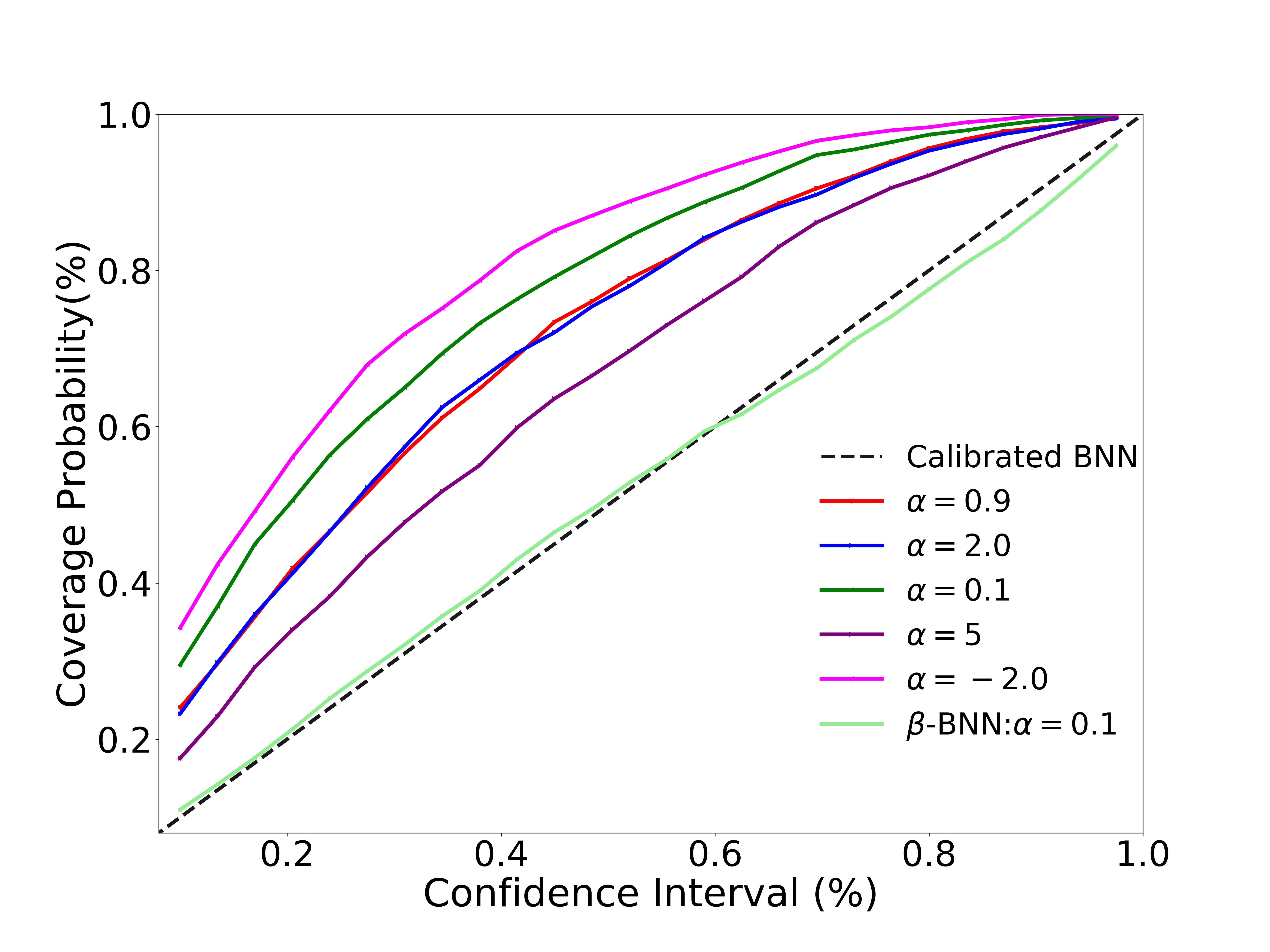
Figure 1: Reliability diagrams for BNNs using different $\alpha$-values without taking any post-process calibration technique.

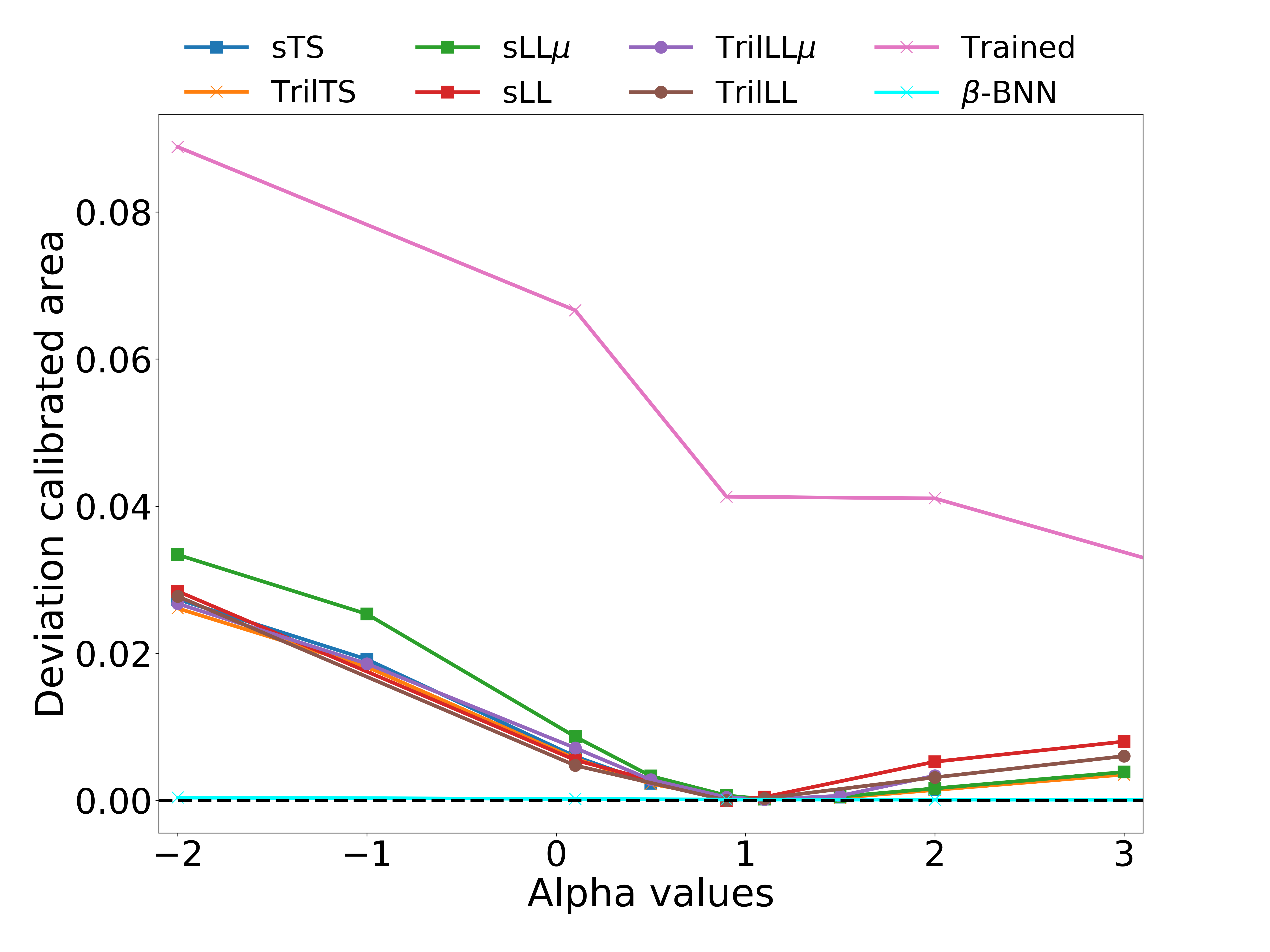
Figure 2: Area between different calibration methods and perfectly calibrated networks. The perfect calibration model corresponds to the $\alpha$-values where occur the intersection of the curves with the solid black line.

In Fig. 2 we report calibration experiments with alpha divergences of the BNN previously trained with standard KL. This figure shows the area between the miscalibrated and perfect calibrated network, where the horizontal black line corresponds to a perfect calibration. As previously observed, the BNNs trained with different alpha divergences do not intersect the black line, i.e. they will not produce calibrated uncertainties. In contrast, all the proposed techniques demonstrate good calibration for some range of alpha around $1$, $\alpha\in[1,1.5]$. This result is consistent with the test NLL measures displayed in Fig. 3, where the values which comes from the post processing methods outperform the ones obtained by the trained BNNs.

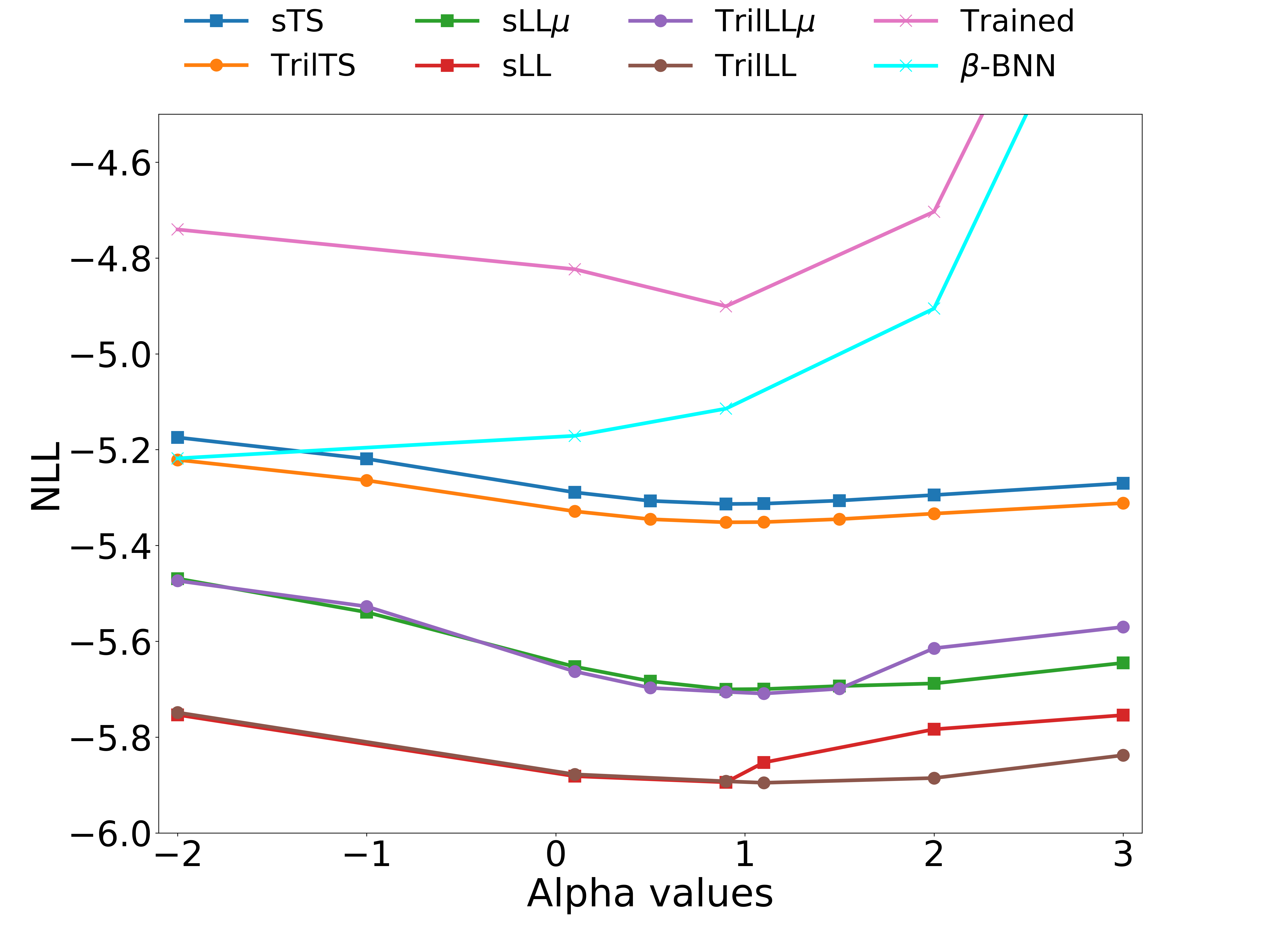
Figure 3: Test NLL of BB-$\alpha$ for both the trained BNN model, and after its post-process calibration.

Moreover, we can observe that LastLayer (LL) usually outperform $\beta$-BNN, and both LastLayermean (LL$\mu$) and Temperature Scaling(TS) in terms of this metric (parameter estimation can be seen in Appendix A.2). Additionally, the NLL achieves a minimum value around $\alpha\approx 1$ where the network is adequately calibrated. The coefficient of determination $R^{2}$ is displayed in Fig. 4. Note that the ability of BNNs to predict the correct outcomes becomes higher for negative $\alpha$ which turns out to be opposite to the NLL behavior. These results are in agreement with (Rodríguez Santana & Hernández-Lobato, 2019), where they report that the choice of $\alpha$ depends on the metric we are most interested in, i.e., when $\alpha\approx 1$, the optimization gives more attention to the NLL resulting in a more accurate predictive distribution, while negative $\alpha$’s focus more on the minimization of the error for predicting the data.

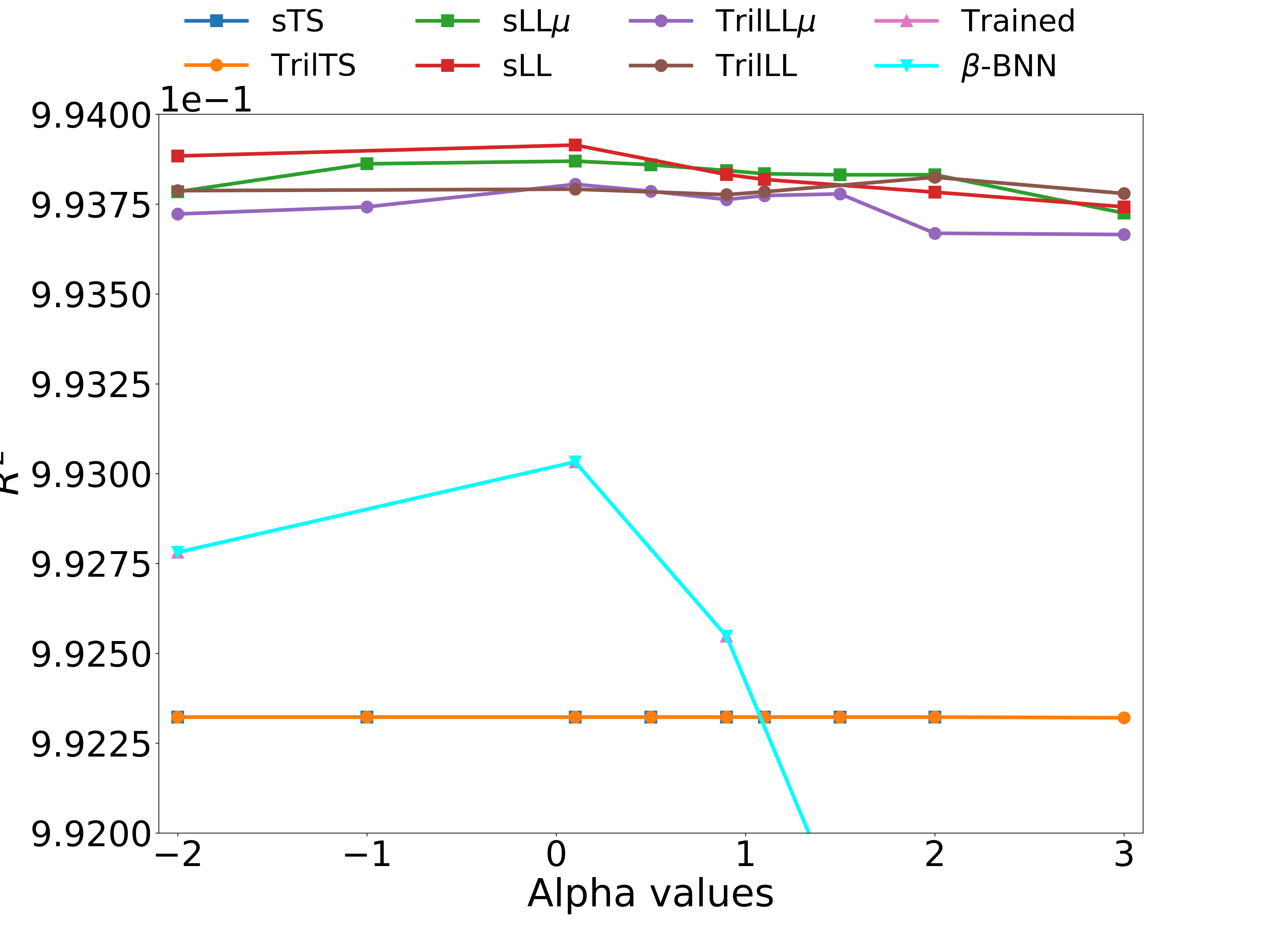
Figure 4: Test $R^{2}$ of BB-$\alpha$ for both the trained BNN model, and after its post-process calibration.

Finally, Fig 5 displays the effect of $\alpha$ on the epistemic uncertainty. As discussed in the previous section TS alone is not able to affect epistemic uncertainty and thus sTS and TrilTS are flat and overlapping. Left aside TS, the epistemic increases with the value of $\alpha$ for all methods. Positive $\alpha$ values tends to cover the entire true posterior, which translate into increasing the variance and hence the epistemic uncertainty. Conversely, negatives $\alpha$ produce smaller epistemic values because the approximate posterior favours the local modes in the true posterior implying less variance. This behaviour of the alpha divergence has been already pointed out in (Minka, 2005).

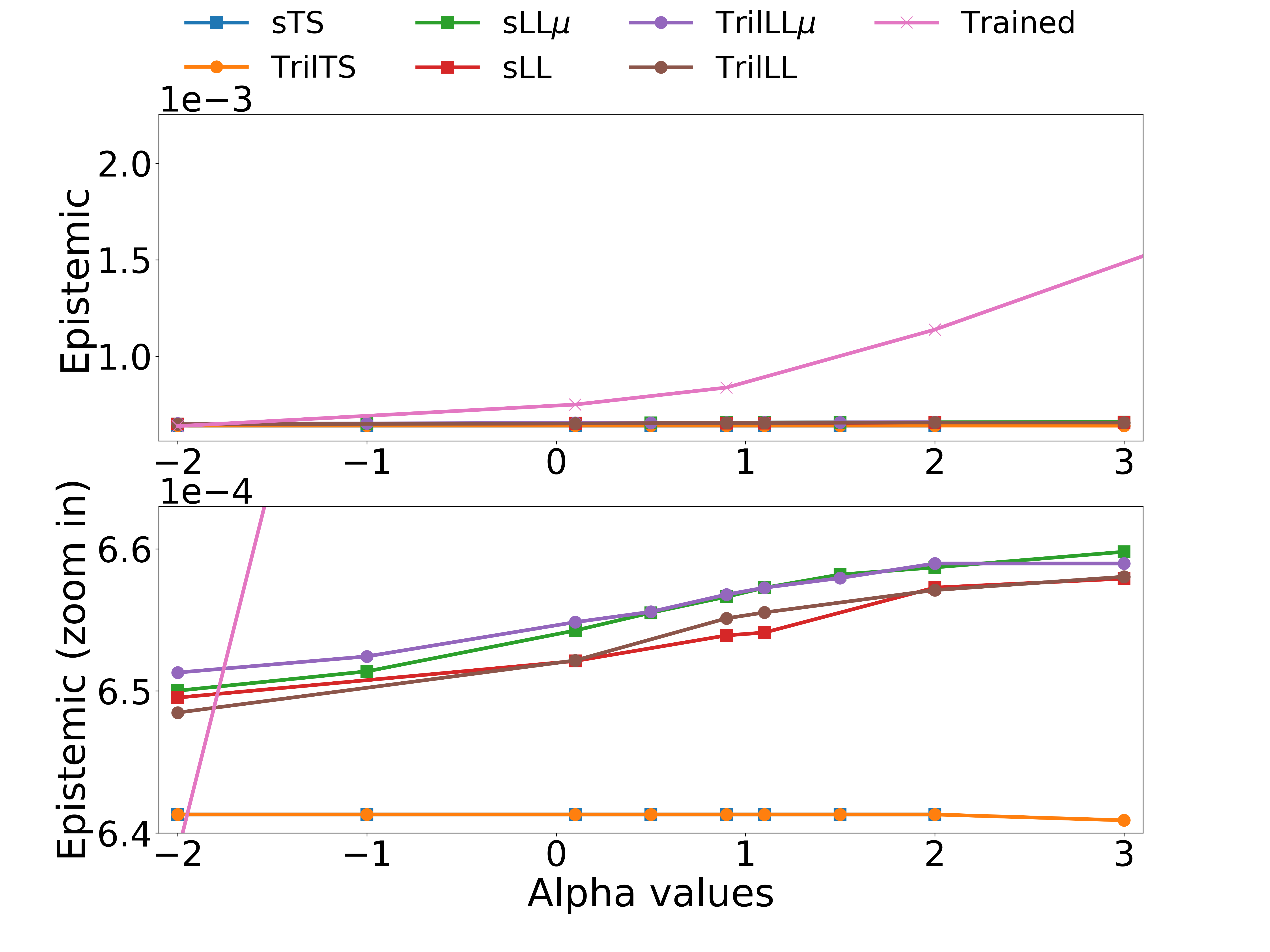
Figure 5: Epistemic uncertainty behavior in post-process calibration scenario.

7 Conclusions

In this paper we have presented an extension of temperature scaling method combined with the use of alpha divergences as a set of calibration techniques for BNNs in regression problems, which improves the performance of the networks both in terms of accurate uncertainties and coefficient of determination $R^{2}$. This approach outperforms the use of alpha divergence in training both without and with beta calibration. Future work will investigate the application of our approach in standard UCI datasets both for regression and classification tasks.

Appendix A Supplemental Materials

A.1 Reliability Diagrams

Reliability diagrams are visual representations of model calibration (Guo et al., 2017). In our case we generate these diagrams by plotting the predicted interval coverage probabilities of the test set. The coverage probabilities are defined as the $x\%$ of samples for which the true value of the parameters falls in the $x\%$-confidence intervals. If the model is perfectly calibrated, then the diagram should plot the identity function, and any deviation from the identity represents miscalibration. For models that produce an approximately Gaussian joint distribution (higher-order statistical moments are very close to zero), one can assume that the predictive distribution obey to a multivariate Gaussian distributions whose confidence region can be computed by

$$\mathcal{C}\geq(\bm{y}-\bm{\hat{y}})^{\top}\Sigma^{-1}(\bm{y}-\bm{\hat{y}}),$$ (7)

which is basically an ellipsoidal confidence set with coverage probability $1-\gamma$. The quantity $\mathcal{C}$ has the Hotelling’s T-squared distribution $T^{2}_{k,D-k}(1-\gamma)/D$, with $k$ degrees of freedom, being $D$ the number of samples (Hortua et al., 2019). In case of unimodal models (not necessarily Gaussian), we can follow the method used in (Perreault Levasseur et al., 2017) where we can generate a histogram from binned samples drawn from the posterior. Since this histogram is expected to be unimodal, we can compute the interval that contains the (100$\alpha$)% of the samples around the mode, with $\alpha\in[0,1]$.

A.2 Parameter model constraints

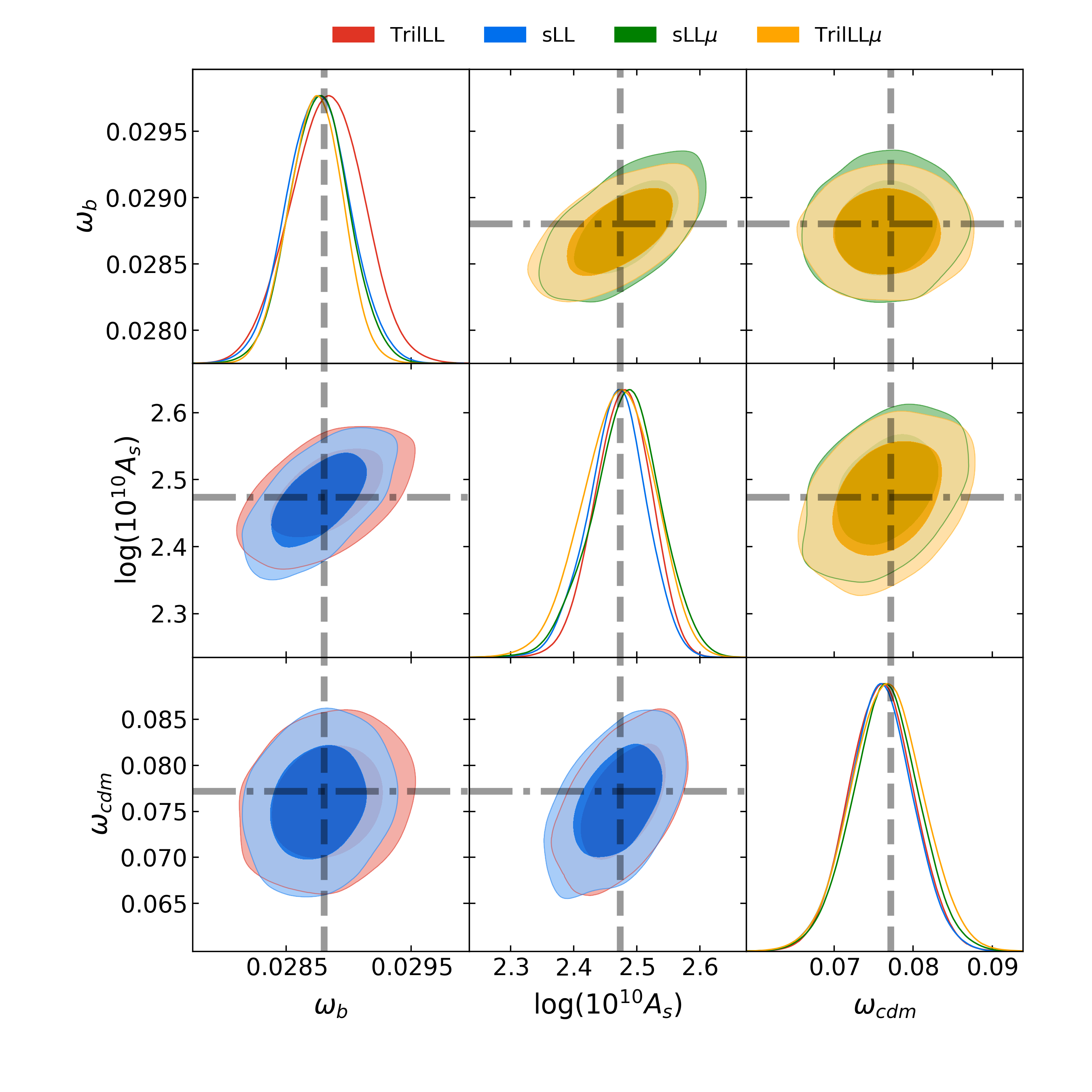
Figure 6: Constraints on parameters of the model from the best calibration approaches. Contours contain 68% and 95% of the probability. The dashed lines represent the true value for an example in the test dataset.

A.3 Reliability diagram for a proposal

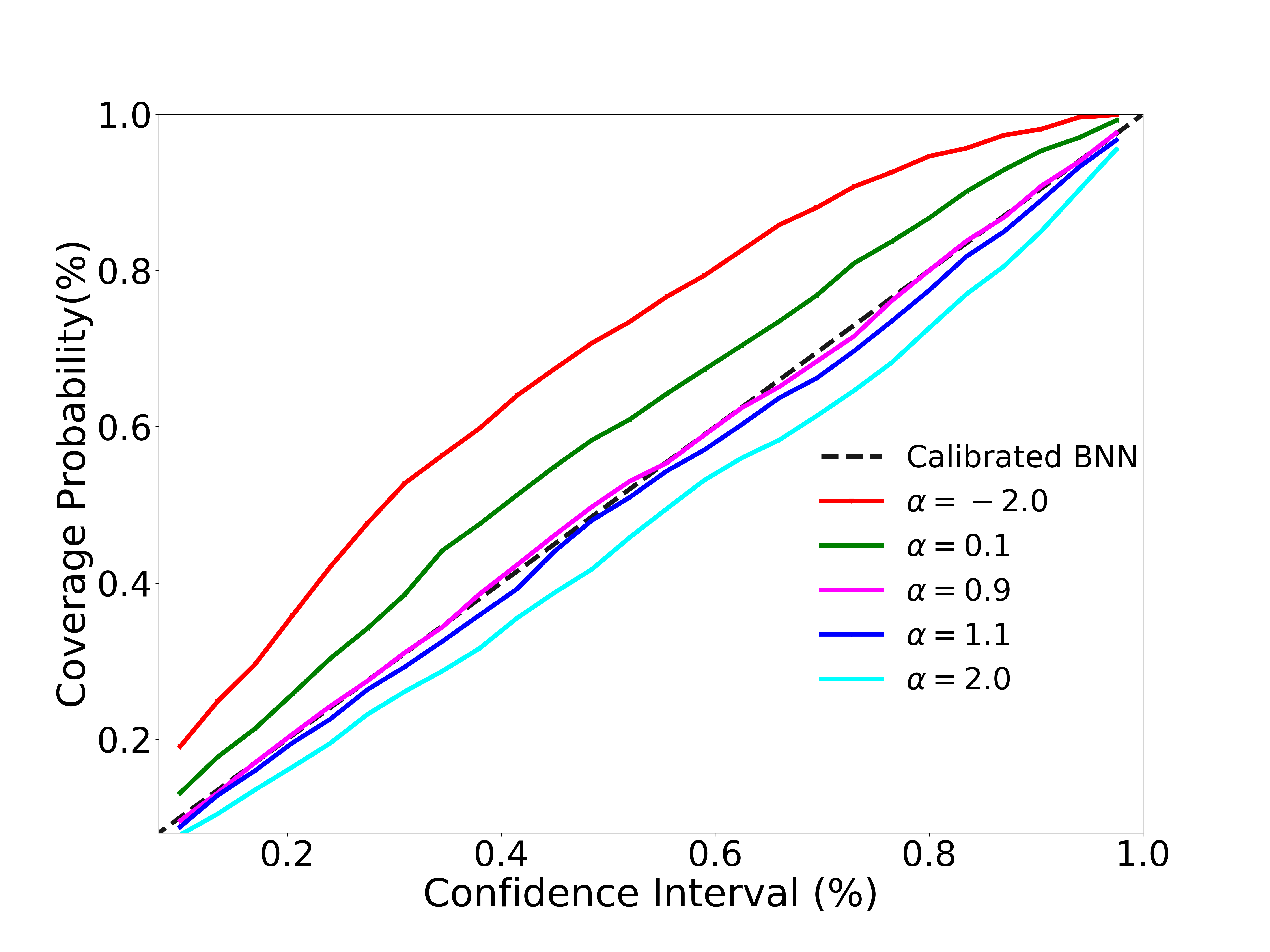
Figure 7: Reliability diagrams for different $\alpha$-values using the TrilLL approach.

References

- Cobb et al. (2019) Cobb, A. D., Himes, M. D., Soboczenski, F., Zorzan, S., O’Beirne, M. D., Baydin, A. G., Gal, Y., Domagal-Goldman, S. D., Arney, G. N., and and, D. A. An ensemble of bayesian neural networks for exoplanetary atmospheric retrieval. The Astronomical Journal, 158(1):33, jun 2019. doi: 10.3847/1538-3881/ab2390. URL https://doi.org/10.3847%2F1538-3881%2Fab2390.
- Dorta et al. (2018) Dorta, G., Vicente, S., Agapito, L., Campbell, N. D. F., and Simpson, I. Structured uncertainty prediction networks. 2018 IEEE/CVF Conference on Computer Vision and Pattern Recognition, Jun 2018. doi: 10.1109/cvpr.2018.00574. URL http://dx.doi.org/10.1109/CVPR.2018.00574.
- Gal & Ghahramani (2016) Gal, Y. and Ghahramani, Z. Bayesian convolutional neural networks with Bernoulli Approximate Variational Inference. In 4th International Conference on Learning Representations (ICLR) workshop track, 2016.
- Graves (2011a) Graves, A. Practical variational inference for neural networks. In Shawe-Taylor, J., Zemel, R. S., Bartlett, P. L., Pereira, F., and Weinberger, K. Q. (eds.), Advances in Neural Information Processing Systems 24, pp. 2348–2356. Curran Associates, Inc., 2011a.
- Graves (2011b) Graves, A. Practical variational inference for neural networks. In Advances in neural information processing systems, pp. 2348–2356, 2011b.
- Guo et al. (2017) Guo, C., Pleiss, G., Sun, Y., and Weinberger, K. Q. On calibration of modern neural networks. In Proceedings of the 34th International Conference on Machine Learning - Volume 70, ICML’17, pp. 1321–1330. JMLR.org, 2017. URL http://dl.acm.org/citation.cfm?id=3305381.3305518.
- Hernández-Lobato et al. (2015) Hernández-Lobato, J. M., Li, Y., Rowland , M., Hernández-Lobato, D., Bui, T., and Turner, R. E. Black-box -divergence Minimization. arXiv e-prints, art. arXiv:1511.03243, November 2015.
- Hinton & van Camp (1993) Hinton, G. E. and van Camp, D. Keeping the neural networks simple by minimizing the description length of the weights. In Proceedings of the Sixth Annual Conference on Computational Learning Theory, COLT ’93, pp. 5–13, New York, NY, USA, 1993. Association for Computing Machinery. ISBN 0897916115. doi: 10.1145/168304.168306. URL https://doi.org/10.1145/168304.168306.
- Hortua et al. (2019) Hortua, H. J., Volpi, R., Marinelli, D., and Malagò, L. Parameters estimation for the cosmic microwave background with bayesian neural networks. arXiv:1911.08508, 2019.
- Kuleshov et al. (2018) Kuleshov, V., Fenner, N., and Ermon, S. Accurate uncertainties for deep learning using calibrated regression, 2018.
- Kull et al. (2017) Kull, M., Filho, T. S., and Flach, P. Beta calibration: a well-founded and easily implemented improvement on logistic calibration for binary classifiers. In Singh, A. and Zhu, J. (eds.), Proceedings of the 20th International Conference on Artificial Intelligence and Statistics, volume 54 of Proceedings of Machine Learning Research, pp. 623–631, Fort Lauderdale, FL, USA, 20–22 Apr 2017. PMLR. URL http://proceedings.mlr.press/v54/kull17a.html.
- Levi et al. (2019) Levi, D., Gispan, L., Giladi, N., and Fetaya, E. Evaluating and Calibrating Uncertainty Prediction in Regression Tasks. arXiv e-prints, art. arXiv:1905.11659, May 2019.
- Li & Gal (2017) Li, Y. and Gal, Y. Dropout inference in bayesian neural networks with alpha-divergences. In Proceedings of the 34th International Conference on Machine Learning-Volume 70, pp. 2052–2061. JMLR. org, 2017.
- Minka (2004) Minka, T. Power ep. Technical Report MSR-TR-2004-149, Microsoft, January 2004. URL https://www.microsoft.com/en-us/research/publication/power-ep/.
- Minka (2005) Minka, T. Divergence measures and message passing. Technical Report MSR-TR-2005-173, Technical Report,Microsoft Research, January 2005.
- Minka (2013) Minka, T. P. Expectation Propagation for approximate Bayesian inference. arXiv e-prints, art. arXiv:1301.2294, January 2013.
- Perreault Levasseur et al. (2017) Perreault Levasseur, L., Hezaveh, Y. D., and Wechsler, R. H. Uncertainties in Parameters Estimated with Neural Networks: Application to Strong Gravitational Lensing. Astrophys. J., 850(1):L7, 2017. doi: 10.3847/2041-8213/aa9704.
- Platt (1999) Platt, J. C. Probabilistic outputs for support vector machines and comparisons to regularized likelihood methods. In ADVANCES IN LARGE MARGIN CLASSIFIERS, pp. 61–74. MIT Press, 1999.
- Rodríguez Santana & Hernández-Lobato (2019) Rodríguez Santana, S. and Hernández-Lobato, D. Adversarial -divergence Minimization for Bayesian Approximate Inference. arXiv e-prints, art. arXiv:1909.06945, September 2019.
- Wen et al. (2018) Wen, Y., Vicol, P., Ba, J., Tran, D., and Grosse, R. Flipout: Efficient pseudo-independent weight perturbations on mini-batches. arXiv preprint arXiv:1803.04386, 2018.
- Zadrozny & Elkan (2001) Zadrozny, B. and Elkan, C. Obtaining calibrated probability estimates from decision trees and naive bayesian classifiers. In Proceedings of the Eighteenth International Conference on Machine Learning, ICML ’01, pp. 609–616, San Francisco, CA, USA, 2001. Morgan Kaufmann Publishers Inc. ISBN 1-55860-778-1. URL http://dl.acm.org/citation.cfm?id=645530.655658.
- Zadrozny & Elkan (2002) Zadrozny, B. and Elkan, C. Transforming classifier scores into accurate multiclass probability estimates. In Proceedings of the Eighth ACM SIGKDD International Conference on Knowledge Discovery and Data Mining, KDD ’02, pp. 694–699, New York, NY, USA, 2002. ACM. ISBN 1-58113-567-X. doi: 10.1145/775047.775151. URL http://doi.acm.org/10.1145/775047.775151.