On the Gauss map of equivariant immersions in hyperbolic space

Abstract.

Given an oriented immersed hypersurface in hyperbolic space $\mathbb{H}^{n+1}$, its Gauss map is defined with values in the space of oriented geodesics of $\mathbb{H}^{n+1}$, which is endowed with a natural para-Kähler structure. In this paper we address the question of whether an immersion $G$ of the universal cover of an $n$-manifold $M$, equivariant for some group representation of $\pi_{1}(M)$ in $\mathrm{Isom}(\mathbb{H}^{n+1})$, is the Gauss map of an equivariant immersion in $\mathbb{H}^{n+1}$. We fully answer this question for immersions with principal curvatures in $(-1,1)$: while the only local obstructions are the conditions that $G$ is Lagrangian and Riemannian, the global obstruction is more subtle, and we provide two characterizations, the first in terms of the Maslov class, and the second (for $M$ compact) in terms of the action of the group of compactly supported Hamiltonian symplectomorphisms.

1. Introduction

The purpose of the present paper is to study immersions of hypersurfaces in the hyperbolic space $\mathbb{H}^{n+1}$, in relation with the geometry of their Gauss maps in the space of oriented geodesics of $\mathbb{H}^{n+1}$. We will mostly restrict to immersions having principal curvatures in $(-1,1)$, and our main aim is to study immersions of $\widetilde{M}$ which are equivariant with respect to some group representation $\rho:\pi_{1}(M)\to\mathrm{Isom}^{+}(\mathbb{H}^{n+1})$, for $M$ a $n$-manifold. The two main results in this direction are Theorem D and Theorem G: the former holds for any $M$, while the latter under the assumption that $M$ is closed.

1.1. Context in literature

In the groundbreaking paper [Hit82], Hitchin observed the existence of a natural complex structure on the space of oriented geodesics in Euclidean three-space. A large interest has then grown on the geometry of the space of oriented (maximal unparametrized) geodesics of Euclidean space of any dimension (see [GK05, Sal05, Sal09, GG14]) and of several other Riemannian and pseudo-Riemannian manifolds (see [AGK11, Anc14, Sep17, Bar18, BS19]). In this paper, we are interested in the case of hyperbolic $n$-space $\mathbb{H}^{n}$, whose space of oriented geodesics is denoted here by $\mathcal{G}(\mathbb{H}^{n})$. The geometry of $\mathcal{G}(\mathbb{H}^{n})$ has been addressed in [Sal07] and, for $n=3$, in [GG10a, GG10b, Geo12, GS15]. For the purpose of this paper, the most relevant geometric structure on $\mathcal{G}(\mathbb{H}^{n})$ is a natural para-Kähler structure $(\mathbbm{G},\mathbbm{J},\Omega)$ (introduced in [AGK11, Anc14]), a notion which we will describe in Section 1.4 of this introduction and more in detail in Section 2.3. A particularly relevant feature of such para-Kähler structure is the fact that the Gauss map of an oriented immersion $\sigma:M\to\mathbb{H}^{n}$, which is defined as the map that associates to a point of $M$ the orthogonal geodesic of $\sigma$ endowed with the compatible orientation, is a Lagrangian immersion in $\mathcal{G}(\mathbb{H}^{n})$. We will come back to this important point in Section 1.2. Let us remark here that, as a consequence of the geometry of the hyperbolic space $\mathbb{H}^{n}$, an oriented geodesic in $\mathbb{H}^{n}$ is characterized, up to orientation preserving reparametrization, by the ordered couple of its “endpoints” in the visual boundary $\partial\mathbb{H}^{n}$: this gives an identification $\mathcal{G}(\mathbb{H}^{n})\cong\partial\mathbb{H}^{n}\times\partial\mathbb{H}^{n}\setminus\Delta$. Under this identification the Gauss map $G_{\sigma}$ of an immersion $\sigma:M\to\mathbb{H}^{n}$ corresponds to a pair of hyperbolic Gauss maps $G_{\sigma}^{\pm}:M\to\partial\mathbb{H}^{n}$.

A parallel research direction, originated by the works of Uhlenbeck [Uhl83] and Epstein [Eps86a, Eps86b, Eps87], concerned the study of immersed hypersurfaces in $\mathbb{H}^{n}$, mostly in dimension $n=3$. These works highlighted the relevance of hypersurfaces satisfying the geometric condition for which principal curvatures are everywhere different from $\pm 1$, sometimes called horospherically convexity: this is the condition that ensures that the hyperbolic Gauss maps $G_{\sigma}^{\pm}$ are locally invertible. On the one hand, Epstein developed this point of view to give a description “from infinity” of horospherically convex hypersurfaces as envelopes of horospheres. This approach has been pursued by many authors by means of analytic techniques, see for instance [Sch02, IdCR06, KS08], and permitted to obtain remarkable classification results often under the assumption that the principal curvatures are larger than 1 in absolute value ([Cur89, AC90, AC93, EGM09, BEQ10, BEQ15, BQZ17, BMQ18]). On the other hand, Uhlenbeck considered the class of so-called almost-Fuchsian manifolds, which has been largely studied in [KS07, GHW10, HL12, HW13, HW15, Sep16, San17] afterwards. These are complete hyperbolic manifolds diffeomorphic to $S\times{\mathbb{R}}$, for $S$ a closed orientable surface of genus $g\geq 2$, containing a minimal surface with principal curvatures different from $\pm 1$. These surfaces lift on the universal cover to immersions $\sigma:\widetilde{S}\to\mathbb{H}^{3}$ which are equivariant for a quasi-Fuchsian representation $\rho:\pi_{1}(S)\to\mathrm{Isom}^{+}(\mathbb{H}^{3})$ and, by the Gauss-Bonnet formula, have principal curvatures in $(-1,1)$, a condition to which we will refer as having small principal curvatures.

1.2. Integrability of immersions in $\mathcal{G}(\mathbb{H}^{n})$

One of the main goals of this paper is to discuss when an immersion $G\colon M^{n}\to\mathcal{G}(\mathbb{H}^{n+1})$ is integrable, namely when it is the Gauss map of an immersion $M\to\mathbb{H}^{n+1}$, in terms of the geometry of $\mathcal{G}(\mathbb{H}^{n+1})$. We will distinguish three types of integrability conditions, which we list from the weakest to the strongest:

• An immersion $G\colon M\to\mathcal{G}(\mathbb{H}^{n+1})$ is locally integrable if for all $p\in M$ there exists a neighbourhood $U$ of $p$ such that $G|_{U}$ is the Gauss map of an immersion $U\to\mathbb{H}^{n+1}$;

• An immersion $G\colon M\to\mathcal{G}(\mathbb{H}^{n+1})$ is globally integrable if it is the Gauss map of an immersion $M\to\mathbb{H}^{n+1}$;

• Given a representation $\rho\colon\pi_{1}(M)\to\mathrm{Isom}^{+}(\mathbb{H}^{n+1})$, a $\rho$-equivariant immersion $G\colon\widetilde{M}\to\mathcal{G}(\mathbb{H}^{n+1})$ is $\rho$-integrable if it is the Gauss map of a $\rho$-equivariant immersion $\widetilde{M}\to\mathbb{H}^{n+1}$.

Let us clarify here that, since the definition of Gauss map requires to fix an orientation on $M$ (see Definition 3.1), the above three definitions of integrability have to be interpreted as: “there exists an orientation on $U$ (in the first case) or $M$ (in the other two) such that $G$ is the Gauss map of an immersion in $\mathbb{H}^{n+1}$ with respect to that orientation”.

We will mostly restrict to immersions $\sigma$ with small principal curvatures, which is equivalent to the condition that the Gauss map $G_{\sigma}$ is Riemannian, meaning that the pull-back by $G_{\sigma}$ of the ambient pseudo-Riemannian metric of $\mathcal{G}(\mathbb{H}^{n+1})$ is positive definite, hence a Riemannian metric (Proposition 4.2).

Local integrability

As it was essentially observed in [Anc14, Theorem 2.10], local integrability admits a very simple characterization in terms of the symplectic geometry of $\mathcal{G}(\mathbb{H}^{n+1})$.

Theorem A.

Let $M^{n}$ be a manifold and $G\colon M\to\mathcal{G}(\mathbb{H}^{n+1})$ be an immersion. Then $G$ is locally integrable if and only if it is Lagrangian.

The methods of this paper easily provide a proof of Theorem A, which is independent from the content of [Anc14]. Let us denote by $T^{1}\mathbb{H}^{n+1}$ the unit tangent bundle of $\mathbb{H}^{n+1}$ and by

$$\mathrm{p}\colon T^{1}\mathbb{H}^{n+1}\to\mathcal{G}(\mathbb{H}^{n+1})~{},$$ (1)

the map such that $\mathrm{p}(x,v)$ is the oriented geodesic of $\mathbb{H}^{n+1}$ tangent to $v$ at $x$. Then, if $G$ is Lagrangian, we prove that one can locally construct maps $\zeta:U\to T^{1}\mathbb{H}^{n+1}$ (for $U$ a simply connected open set) such that $\mathrm{p}\circ\zeta=G$. Up to restricting the domain again, one can find such a $\zeta$ so that it projects to an immersion $\sigma$ in $\mathbb{H}^{n+1}$ (Lemma 5.8), and the Gauss map of $\sigma$ is $G$ by construction.

Our next results are, to our knowledge, completely new and give characterizations of global integrability and $\rho$-integrability under the assumption of small principal curvatures.

Global integrability

The problem of global integrability is in general more subtle than local integrability. As a matter of fact, in Example 5.9 we construct an example of a locally integrable immersion $G:(-T,T)\to\mathcal{G}(\mathbb{H}^{2})$ that is not globally integrable. By taking a cylinder on this curve, one easily sees that the same phenomenon occurs in any dimension. We stress that in our example $M=(-T,T)$ (or the product $(-T,T)\times{\mathbb{R}}^{n-1}$ for $n>2$) is simply connected: the key point in our example is that one can find globally defined maps $\zeta:M\to T^{1}\mathbb{H}^{n+1}$ such that $G=\mathrm{p}\circ\zeta$, but no such $\zeta$ projects to an immersion in $\mathbb{H}^{n+1}$.

Nevertheless, we show that this issue does not occur for Riemannian immersions $G$. In this case any immersion $\sigma$ whose Gauss map is $G$ (if it exists) necessarily has small principal curvatures. We will always restrict to this setting hereafter. In summary, we have the following characterization of global integrability for $M$ simply connected:

Theorem B.

Let $M^{n}$ be a simply connected manifold and $G\colon M\to\mathcal{G}(\mathbb{H}^{n+1})$ be a Riemannian immersion. Then $G$ is globally integrable if and only if it is Lagrangian.

We give a characterization of global integrability for $\pi_{1}(M)\neq\{1\}$ in Corollary E, which is a direct consequence of our first characterization of $\rho$-integrability (Theorem D). Anyway, we remark that if a Riemannian and Lagrangian immersion $G\colon M\to\mathcal{G}(\mathbb{H}^{n+1})$ is also complete (i.e. has complete first fundamental form), then $M$ is necessarily simply connected:

Theorem C.

Let $M^{n}$ be a manifold. If $G\colon M\to\mathcal{G}(\mathbb{H}^{n+1})$ is a complete Riemannian and Lagrangian immersion, then $M$ is diffeomorphic to ${\mathbb{R}}^{n}$ and $G$ is the Gauss map of a proper embedding $\sigma:M\to\mathbb{H}^{n+1}$.

In Theorem C the conclusion that $G=G_{\sigma}$ for $\sigma$ a proper embedding follows from the fact that $\sigma$ is complete, which is an easy consequence of Equation (24) relating the first fundamental forms of $\sigma$ and $G_{\sigma}$, and the non-trivial fact that complete immersions in $\mathbb{H}^{n+1}$ with small principal curvatures are proper embeddings (Proposition 4.15).

$\rho$-integrability

Let us first observe that the problem of $\rho$-integrability presents some additional difficulties than global integrability. Assume $G\colon\widetilde{M}\to\mathcal{G}(\mathbb{H}^{n+1})$ is a Lagrangian, Riemannian and $\rho$-equivariant immersion for some representation $\rho\colon\pi_{1}(M^{n})\to\mathrm{Isom}^{+}(\mathbb{H}^{n+1})$. Then, by Theorem B, there exists $\sigma\colon\widetilde{M}\to\mathbb{H}^{n+1}$ with Gauss map $G$, but the main issue is that such a $\sigma$ will not be $\rho$-equivariant in general, as one can see in Examples 6.1 and 6.2.

Nevertheless, $\rho$-integrability of Riemannian immersions into $\mathcal{G}(\mathbb{H}^{n+1})$ can still be characterized in terms of their extrinsic geometry. Let $\overline{\mathrm{H}}$ be the mean curvature vector of $G$, defined as the trace of the second fundamental form, and $\Omega$ the symplectic form of $\mathcal{G}(\mathbb{H}^{n+1})$. Since $G$ is $\rho$-equivariant, the $1$-form $G^{*}(\Omega(\overline{\mathrm{H}},\cdot))$ on $\widetilde{M}$ is invariant under the action of $\pi_{1}(M)$, so it descends to a $1$-form on $M$. One can prove that such $1$-form on $M$ is closed (Corollary 6.7): we will denote its cohomology class in $H^{1}_{dR}(M,{\mathbb{R}})$ with $\mu_{G}$ and we will call it the Maslov class of $G$, in accordance with some related interpretations of the Maslov class in other geometric contexts (see among others [Mor81, Oh94, Ars00, Smo02]). The Maslov class encodes the existence of equivariantly integrating immersions, in the sense stated in the following theorem.

Theorem D.

Let $M^{n}$ be an orientable manifold, $\rho\colon\pi_{1}(M)\to\mathrm{Isom}^{+}(\mathbb{H}^{n+1})$ be a representation and $G\colon\widetilde{M}\to\mathcal{G}(\mathbb{H}^{n+1})$ be a $\rho$-equivariant Riemannian and Lagrangian immersion. Then $G$ is $\rho$-integrable if and only if the Maslov class $\mu_{G}$ vanishes.

Applying Theorem D to a trivial representation, we immediately obtain a characterization of global integrability for Riemannian immersions, thus extending Theorem B to the case $\pi_{1}(M)\neq\{1\}$.

Corollary E.

Let $M^{n}$ be an orientable manifold and $G\colon M\to\mathcal{G}(\mathbb{H}^{n+1})$ be a Riemannian and Lagrangian immersion. Then $G$ is globally integrable if and only if its Maslov class $\mu_{G}$ vanishes.

1.3. Nearly-Fuchsian representations

Let us now focus on the case of $M$ a closed oriented manifold. Although our results apply to any dimension, we borrow the terminology from the three-dimensional case (see [HW13]) and say that a representation $\rho\colon\pi_{1}(M)\to\mathrm{Isom}^{+}(\mathbb{H}^{n+1})$ is nearly-Fuchsian if there exists a $\rho$-equivariant immersion $\sigma\colon\widetilde{M}\to\mathbb{H}^{n+1}$ with small principal curvatures. We show (Proposition 4.18) that the action of a nearly-Fuchsian representation on $\mathbb{H}^{n+1}$ is free, properly discontinuously and convex cocompact; the quotient of $\mathbb{H}^{n+1}$ by $\rho(\pi_{1}(M))$ is called nearly-Fuchsian manifold.

Moreover, the action of $\rho(\pi_{1}(M))$ extends to a free and properly discontinuous action on the complement of a topological $(n-1)$-sphere $\Lambda_{\rho}$ (the limit set of $\rho$) in the visual boundary $\partial\mathbb{H}^{n+1}$. Such complement is the disjoint union of two topological $n$-discs which we denote by $\Omega_{+}$ and $\Omega_{-}$. It follows that there exists a maximal open region of $\mathcal{G}(\mathbb{H}^{n+1})$ over which a nearly-Fuchsian representation $\rho$ acts freely and properly discontinuously. This region is defined as the subset of $\mathcal{G}(\mathbb{H}^{n+1})$ consisting of oriented geodesics having either final endpoint in $\Omega_{+}$ or initial endpoint in $\Omega_{-}$. The quotient of this open region via the action of $\rho$, that we denote with $\mathcal{G}_{\rho}$, inherits a para-Kähler structure.

Let us first state a uniqueness result concerning nearly-Fuchsian representations. A consequence of Theorem D and the definition of Maslov class is that if $G$ is a $\rho$-equivariant, Riemannian and Lagrangian immersion which is furthermore minimal, i.e. with $\overline{\mathrm{H}}=0$, then it is $\rho$-integrable. Together with an application of a maximum principle in the corresponding nearly-Fuchsian manifold, we prove:

Corollary F.

Given a closed orientable manifold $M^{n}$ and a representation $\rho:\pi_{1}(M)\to\mathrm{Isom}^{+}(\mathbb{H}^{n+1})$, there exists at most one $\rho$-equivariant Riemannian minimal Lagrangian immersion $G:\widetilde{M}\to\mathcal{G}(\mathbb{H}^{n+1})$ up to reparametrization. If such a $G$ exists, then $\rho$ is nearly-Fuchsian and $G$ induces a minimal Lagrangian embedding of $M$ in $\mathcal{G}_{\rho}$.

In fact, for any $\rho$-equivariant immersion $\sigma:\widetilde{M}\to\mathbb{H}^{n+1}$ with small principal curvatures, the hyperbolic Gauss maps $G_{\sigma}^{\pm}$ are equivariant diffeomorphisms between $\widetilde{M}$ and $\Omega_{\pm}$. Hence up to changing the orientation of $M$, which corresponds to swapping the two factors $\partial\mathbb{H}^{n+1}$ in the identification $\mathcal{G}(\mathbb{H}^{n+1})\cong\partial\mathbb{H}^{n+1}\times\partial\mathbb{H}^{n+1}\setminus\Delta$, the Gauss map of $\sigma$ takes values in the maximal open region defined above, and induces an embedding of $M$ in $\mathcal{G}_{\rho}$.

This observations permits to deal (in the cocompact case) with embeddings in $\mathcal{G}_{\rho}$ instead of $\rho$-equivariant embeddings in $\mathcal{G}(\mathbb{H}^{n+1})$. In analogy with the definition of $\rho$-integrability defined above, we will say that a $n$-dimensional submanifold $\mathcal{L}\subset\mathcal{G}_{\rho}$ is $\rho$-integrable if it is the image in the quotient of a $\rho$-integrable embedding in $\mathcal{G}(\mathbb{H}^{n+1})$. Clearly such $\mathcal{L}$ is necessarily Lagrangian by Theorem A. We are now ready to state our second characterization result for $\rho$-integrability .

Theorem G.

Let $M$ be a closed orientable $n$-manifold, $\rho:\pi_{1}(M)\to\mathrm{Isom}^{+}(\mathbb{H}^{n+1})$ be a nearly-Fuchsian representation and $\mathcal{L}\subset\mathcal{G}_{\rho}$ a Riemannian $\rho$-integrable submanifold. Then a Riemannian submanifold $\mathcal{L}^{\prime}$ is $\rho$-integrable if and only if there exists $\Phi\in\mathrm{Ham}_{c}(\mathcal{G}_{\rho},\Omega)$ such that $\Phi(\mathcal{L})=\mathcal{L}^{\prime}$.

In Theorem G we denoted by $\mathrm{Ham}_{c}(\mathcal{G}_{\rho},\Omega)$ the group of compactly-supported Hamiltonian symplectomorphisms of $\mathcal{G}_{\rho}$ with respect to its symplectic form $\Omega$. (See Definition 7.2). The proof of Theorem G in fact shows that if $\mathcal{L}$ is $\rho$-integrable and $\mathcal{L}^{\prime}=\Phi(\mathcal{L})$ for $\Phi\in\mathrm{Ham}_{c}(\mathcal{G}_{\rho},\Omega)$, then $\mathcal{L}^{\prime}$ is integrable as well, even without the hypothesis that $\mathcal{L}$ and $\mathcal{L}^{\prime}$ are Riemannian submanifolds.

If $\rho$ admits an equivariant Riemannian minimal Lagrangian immersion, then Theorem G can be restated by saying that a Riemannian and Lagrangian submanifold $\mathcal{L}^{\prime}$ is $\rho$-integrable if and only if it is in the $\mathrm{Ham}_{c}(\mathcal{G}_{\rho},\Omega)$-orbit of the minimal Lagrangian submanifold $\mathcal{L}\subset\mathcal{G}_{\rho}$, which is unique by Theorem F.

1.4. The geometry of $\mathcal{G}(\mathbb{H}^{n})$ and $T^{1}\mathbb{H}^{n}$

Let us now discuss more deeply the geometry of the space of oriented geodesics of $\mathbb{H}^{n}$ and some of the tools involved in the proofs. In this paper we give an alternative construction of the para-Kähler structure of $\mathcal{G}(\mathbb{H}^{n})$ with respect to the previous literature ([Sal07, GG10b, AGK11, Anc14]), which is well-suited for the problem of (equivariant) integrability. The geodesic flow induces a natural principal ${\mathbb{R}}$-bundle structure whose total space is $T^{1}\mathbb{H}^{n+1}$ and whose bundle map is $\mathrm{p}:T^{1}\mathbb{H}^{n+1}\to\mathcal{G}(\mathbb{H}^{n+1})$ defined in Equation (1), and acts by isometries of the para-Sasaki metric $g$, which is a pseudo-Riemannian version of the classical Sasaki metric on $T^{1}\mathbb{H}^{n+1}$. Let us denote by $\chi$ the infinitesimal generator of the geodesic flow, which is a vector field on $T^{1}\mathbb{H}^{n+1}$ tangent to the fibers of $\mathrm{p}$. The idea is to define each element that constitutes the para-Kähler structure of $\mathcal{G}(\mathbb{H}^{n+1})$ (see the items below) by push-forward of certain tensorial quantities defined on the $g$-orthogonal complement of $\chi$, showing that the push-forward is well defined by invariance under the action of the geodesic flow. More concretely:

• The pseudo-Riemannian metric $\mathbbm{G}$ of $\mathcal{G}(\mathbb{H}^{n+1})$ (of signature $(n,n)$) is defined as push-forward of the restriction of $g$ to $\chi^{\perp}$;

• The para-complex structure $\mathbbm{J}$ (that is, a $(1,1)$ tensor whose square is the identity and whose $\pm 1$-eigenspaces are integrable distributions of the same dimension) is obtained from an endomorphism $J$ of $\chi^{\perp}$, invariant under the geodesic flow, which essentially switches the horizontal and vertical distributions in $T^{1}\mathbb{H}^{n+1}$;

• The symplectic form $\Omega$ arises from a similar construction on $\chi^{\perp}$, in such a way that $\Omega(X,Y)=\mathbbm{G}(X,\mathbb{J}Y)$.

It is worth mentioning that in dimension 3, the pseudo-Riemannian metric $\mathbbm{G}$ of $\mathcal{G}(\mathbb{H}^{3})$ can be seen as the real part of a holomorphic Riemannian manifold of constant curvature $-1$, see [BE20].

The symplectic geometry of $\mathcal{G}(\mathbb{H}^{n+1})$ has a deep relation with the structure of $T^{1}\mathbb{H}^{n+1}$. Indeed the total space of $T^{1}\mathbb{H}^{n+1}$ is endowed with a connection form $\omega$, whose kernel consists precisely of $\chi^{\perp}$ (See Definition 5.1). In Proposition 5.4 we prove the following fundamental relation between the curvature of $\mathrm{p}$ and the symplectic form $\Omega$:

$$d\omega=\mathrm{p}^{*}\Omega~{}.$$ (2)

This identity is an essential point in the proofs of our main results, which we now briefly outline.

1.5. Overview of the proofs

Let us start by Theorem A, namely the equivalence between locally integrable and Lagrangian. Given a locally integrable immersion $G:M\to\mathcal{G}(\mathbb{H}^{n+1})$, the corresponding (local) immersions $\sigma:U\to\mathbb{H}^{n+1}$ provide flat sections of the principal ${\mathbb{R}}$-bundle obtained by pull-back of the bundle $\mathrm{p}:T^{1}\mathbb{H}^{n+1}\to\mathcal{G}(\mathbb{H}^{n+1})$ by $G$. Hence the obstruction to local integrability is precisely the curvature of the pull-back bundle $G^{*}\mathrm{p}$. By Equation (2), it follows that the vanishing of $G^{*}\Omega$ is precisely the condition that characterizes local integrability of $G$.

Moreover, $\rho$-integrability of a $\rho$-equivariant Lagrangian immersion $G:\widetilde{M}\to\mathcal{G}(\mathbb{H}^{n+1})$ can be characterized by the condition that the quotient of the bundle $G^{*}\mathrm{p}$ by the action of $\pi_{1}(M)$ induced by $\rho$ is a trivial flat bundle over $M$, meaning that it admits a global flat section. Once these observations are established, Theorem D will be deduced as a consequence of Theorem 6.12 which states that $\mu_{G}$ is dual, in the sense of de Rham Theorem, to the holonomy of such flat bundle over $M$. In turn, Theorem 6.12 relies on the important expression (proved in Proposition 6.5):

$$G_{\sigma}^{*}(\Omega(\overline{\mathrm{H}},\cdot))=df_{\sigma}~{},$$ (3)

where $G_{\sigma}$ is the Gauss map of an immersion $\sigma$ in $\mathbb{H}^{n+1}$ and $f_{\sigma}$ is the function defined by

$$f_{\sigma}=\frac{1}{n}\sum_{i=1}^{n}\mathrm{arctanh}\lambda_{i}~{}.$$ (4)

where $\lambda_{1},\ldots,\lambda_{n}$ are the principal curvatures of $\sigma$.

Let us move on to a sketch of the proof of Theorem G, which again relies on the reformulation of $\rho$-integrability in terms of triviality of flat bundles. Assuming that $\mathcal{L}$ is a $\rho$-integrable submanifold of $\mathcal{G}_{\rho}$ and that we have a Lagrangian isotopy connecting $\mathcal{L}$ to another Lagrangian submanifold $\mathcal{L}^{\prime}$, Proposition 7.5 states that the holonomy of the flat bundle associated to $\mathcal{L}^{\prime}$ is dual, again in the sense of de Rham Theorem, to the cohomology class of a 1-form which is built out of the Lagrangian isotopy, by a variant for Lagrangian submanifolds of the so-called flux homomorphism. This variant has been developed in [Sol13] and applied in [BS19] for a problem in the Anti-de Sitter three-dimensional context which is to some extent analogous to those studied here. However, in those works stronger topological conditions are assumed which are not applicable here, and therefore our proof of Theorem G uses independent methods.

To summarize the proof, one implication is rather straightforward: if there exists a compactly supported Hamiltonian symplectomorphism $\Phi$ mapping $\mathcal{L}$ to $\mathcal{L}^{\prime}$, then a simple computation shows that the flux homomorphism vanishes along the Hamiltonian isotopy connecting the identity to $\Phi$. This implication does not even need the assumption that $\mathcal{L}$ and $\mathcal{L}^{\prime}$ are Riemannian submanifolds. The most interesting implication is the converse one: assuming that both $\mathcal{L}$ and $\mathcal{L}^{\prime}$ are Riemannian and integrable, we use a differential geometric construction in $\mathbb{H}^{n+1}$ to produce an interpolation between the corresponding hypersurfaces in the nearly-Fuchsian manifold associated to $\rho$. For technical reasons, we need to arrange such interpolation by convex hypersurfaces (Lemma 7.8). An extension argument then provides the time-depending Hamiltonian function whose time-one flow is the desired symplectomorphism $\Phi\in\mathrm{Ham}_{c}(\mathcal{G}_{\rho},\Omega)$ such that $\Phi(\mathcal{L})=\mathcal{L}^{\prime}$.

1.6. Relation with geometric flows

Finally, in Appendix A we apply these methods to study the relation between evolutions by geometric flows in $\mathbb{H}^{n+1}$ and in $\mathcal{G}(\mathbb{H}^{n+1})$. More precisely, suppose that $\sigma_{\bullet}:M\times(-\epsilon,\epsilon)\to\mathbb{H}^{n+1}$ is a smoothly varying family of Riemannian immersions that satisfy:

$$\frac{d}{dt}\sigma_{t}=f_{t}\nu_{t}$$

where $\nu_{t}$ is the normal vector of $\sigma_{t}$ and $f_{\bullet}:M\times(-\epsilon,\epsilon)\to{\mathbb{R}}$ is a smooth function. Then the variation of the Gauss map $G_{t}$ of $\sigma_{t}$ is given, up to a tangential term, by the normal term $-\mathbbm{J}(dG_{t}({\overline{\nabla}}{}^{t}f_{t}))$, where ${\overline{\nabla}}{}^{t}f_{t}$ denotes the gradient with respect to the first fundamental form of $G_{t}$, that is, the Riemannian metric $G_{t}^{*}\mathbbm{G}$.

Let us consider the special case of the function $f_{t}:=f_{\sigma_{t}}$, as defined in Equation (4), namely the sum of hyperbolic inverse tangent of the principal curvatures. The study of the associated flow has been suggested in dimension three in [And02], by analogy of a similar flow on surfaces in the three-sphere. Combining the aforementioned result of Appendix A with Equation (3), we obtain that such flow in $\mathbb{H}^{n+1}$ induces the Lagrangian mean curvature flow in $\mathcal{G}(\mathbb{H}^{n+1})$ up to tangential diffeomorphisms. A similar result has been obtained in Anti-de Sitter space (in dimension three) in [Smo13].

Organization of the paper

The paper is organized as follows. In Section 2 we introduce the space of geodesics $\mathcal{G}(\mathbb{H}^{n+1})$ and its natural para-Kähler structure. In Section 3 we study the properties of the Gauss map and provide useful examples. Section 4 focuses on immersions with small principal curvatures and prove several properties. In Section 5 we study the relations with the geometry of flat principal bundles, in particular Equation (2) (Proposition 5.4, that relies the symplectic form in the space of geodesics to the curvature of principal bundles), and we prove the statements concerning local integrability and global integrability of Riemannian immersions in $\mathcal{G}(\mathbb{H}^{n+1})$, including Theorem A, Theorem B and Theorem C. In Section 6 we discuss the problem of equivariant integrability in relation with the Maslov class of the immersion: we prove Theorem D (more precisely, the stronger version given in Theorem 6.12) and deduce Corollaries E and F. Finally, in Section 7, focusing on nearly-Fuchsian representations, we prove Theorem G.

Acknowledgements

We are grateful to Francesco Bonsante for many related discussion and for his interest and encouragement in this work. Part of this work has been done during visits of the first author to the University of Luxembourg in November 2018 and to Grenoble Alpes University in April-May 2019; we are thankful to these Institutions for the hospitality. We would like to thank an anonymous referee for several useful comments.

2. The space of geodesics of hyperbolic space

In this section, we introduce the hyperbolic space $\mathbb{H}^{n}$ and its space of (oriented maximal unparametrized) geodesics, which will be endowed with a natural para-Kähler structure by means of a construction on the unit tangent bundle $T^{1}\mathbb{H}^{n}$.

2.1. Hyperboloid model

In this paper we will mostly use the hyperboloid model of $\mathbb{H}^{n}$. Let us denote by ${\mathbb{R}}^{n,1}$ the $(n+1)$-dimensional Minkowski space, namely the vector space ${\mathbb{R}}^{n+1}$ endowed with the standard bilinear form of signature $(n,1)$:

$$\langle x,y\rangle=x_{1}y_{1}+\ldots+x_{n}y_{n}-x_{n+1}y_{n+1}~{}.$$

The hyperboloid model of hyperbolic space is

$$\mathbb{H}^{n}=\{x\in{\mathbb{R}}^{n,1}\,|\,\langle x,x\rangle=-1,\,x_{n+1}>0\}~{}.$$

Then the tangent space at a point $x$ is identified to its orthogonal subspace:

$$T_{x}\mathbb{H}^{n}\cong x^{\perp}=\{v\in{\mathbb{R}}^{n,1}\,|\,\langle x,v\rangle=0\}~{}.$$

The unit tangent bundle of $\mathbb{H}^{n}$ is the bundle of unit tangent vectors, and therefore has the following model:

$$T^{1}\mathbb{H}^{n}=\{(x,v)\in{\mathbb{R}}^{n,1}\times{\mathbb{R}}^{n,1}\,|\,x\in\mathbb{H}^{n},\,\langle x,v\rangle=0,\,\langle v,v\rangle=1\}~{},$$ (5)

where the obvious projection map is simply

$$\pi:T^{1}\mathbb{H}^{n}\to\mathbb{H}^{n}\qquad\pi(x,v)=x~{}.$$

In this model, we can give a useful description of the tangent space of $T^{1}\mathbb{H}^{n}$ at a point $(x,v)$, namely:

$$T_{(x,v)}T^{1}\mathbb{H}^{n}=\{(\dot{x},\dot{v})\in{\mathbb{R}}^{n,1}\times{\mathbb{R}}^{n,1}\,|\,\langle x,\dot{x}\rangle=\langle v,\dot{v}\rangle=\langle x,\dot{v}\rangle+\langle v,\dot{x}\rangle=0\}~{},$$ (6)

where the relations $\langle x,\dot{x}\rangle=0$ and $\langle v,\dot{v}\rangle=0$ arise by differentiating $\langle x,x\rangle=-1$ and $\langle v,v\rangle=1$, while the relation $\langle x,\dot{v}\rangle+\langle v,\dot{x}\rangle=0$ is the linearized version of $\langle x,v\rangle=0$.

Finally, let us denote by $\mathcal{G}(\mathbb{H}^{n})$ the space of (maximal, oriented, unparameterized) geodesics of $\mathbb{H}^{n}$, namely, the space of non-constant geodesics $\gamma:{\mathbb{R}}\to\mathbb{H}^{n}$ up to monotone increasing reparameterizations. Recalling that an oriented geodesic is uniquely determined by its two (different) endpoints in the visual boundary $\partial\mathbb{H}^{n}$, we have the following identification of this space:

$$\mathcal{G}(\mathbb{H}^{n})\cong\partial\mathbb{H}^{n}\times\partial\mathbb{H}^{n}\setminus\Delta~{},$$

where $\Delta$ represents the diagonal. We recall that, in the hyperboloid model, $\partial\mathbb{H}^{n}$ can be identified to the projectivization of the null-cone in Minkowski space:

$$\partial\mathbb{H}^{n}=\faktor{\{x\in{\mathbb{R}}^{n,1}\,|\,\langle x,x\rangle=0,\,x_{n+1}>0\}}{{\mathbb{R}}_{>0}}~{}.$$ (7)

It will be of fundamental importance in the following to endow $T^{1}\mathbb{H}^{n}$ with another bundle structure, a principal bundle structure, over $\mathcal{G}(\mathbb{H}^{n})$. For this purpose, recall that the geodesic flow is the ${\mathbb{R}}$-action over $T^{1}\mathbb{H}^{n}$ given by:

$$t\cdot(x,v)=\varphi_{t}(x,v)=(\gamma(t),\gamma^{\prime}(t))~{},$$

where $\gamma$ is the unique parameterized geodesic such that $\gamma(0)=x$ and $\gamma^{\prime}(0)=v$. In the hyperboloid model, the flow $\varphi_{t}\colon T^{1}\mathbb{H}^{n}\to T^{1}\mathbb{H}^{n}$ can be written explicitly as

$$\varphi_{t}(x,v)=(\cosh(t)x+\sinh(t)v,\sinh(t)x+\cosh(t)v)~{}.$$ (8)

Then $T^{1}\mathbb{H}^{n}$ is naturally endowed with a principal ${\mathbb{R}}$-bundle structure:

$$\mathrm{p}:T^{1}\mathbb{H}^{n}\to\mathcal{G}(\mathbb{H}^{n})\qquad\mathrm{p}(x,v)=\gamma~{},$$

for $\gamma$ the geodesic defined as above, that is, $\mathrm{p}(x,v)$ is the element of $\mathcal{G}(\mathbb{H}^{n})$ going through $x$ with speed $v$.

Finally, recall that the group of orientation-preserving isometries of $\mathbb{H}^{n}$, which we will denote by $\mathrm{Isom}^{+}(\mathbb{H}^{n})$, is identified to $\mathrm{SO}_{0}(n,1)$, namely the connected component of the identity in the group of linear isometries of ${\mathbb{R}}^{n,1}$. Clearly $\mathrm{Isom}^{+}(\mathbb{H}^{n})$ acts both on $T^{1}\mathbb{H}^{n}$ and on $\mathcal{G}(\mathbb{H}^{n})$, in the obvious way, and moreover the two projection maps $\pi:T^{1}\mathbb{H}^{n}\to\mathbb{H}^{n}$ and $\mathrm{p}:T^{1}\mathbb{H}^{n}\to\mathcal{G}(\mathbb{H}^{n})$ are equivariant with respect to these actions. In the next sections, we will introduce some additional structures on $T^{1}\mathbb{H}^{n}$ and $\mathcal{G}(\mathbb{H}^{n})$ that are natural in the sense that they are preserved by the action of $\mathrm{Isom}^{+}(\mathbb{H}^{n})$.

2.2. Para-Sasaki metric on the unit tangent bundle

We shall now introduce a pseudo-Riemannian metric on $T^{1}\mathbb{H}^{n}$. For this purpose, let us first recall the construction of the horizontal and vertical lifts and distributions in the unit tangent bundle of a Riemannian manifold, which for simplicity we only recall for $\mathbb{H}^{n}$. Given $(x,v)\in T\mathbb{H}^{n}$, the vertical subspace at $(x,v)$ is defined as:

$$\mathcal{V}^{0}_{(x,v)}=T_{(x,v)}\big{(}\pi^{-1}(x)\big{)}\cong v^{\perp}\subset T_{x}\mathbb{H}^{n}$$

since $\pi^{-1}(x)$ is naturally identified to the sphere of unit vectors in the vector space $T_{x}\mathbb{H}^{n}$. Hence given a vector $w\in T_{x}\mathbb{H}^{n}$ orthogonal to $v$, we can define its vertical lift $w^{\mathcal{V}}\in\mathcal{V}^{0}_{(x,v)}$, and vertical lifting gives a map from $v^{\perp}$ to $\mathcal{V}^{0}_{(x,v)}\subset T_{(x,v)}T^{1}\mathbb{H}^{n}$ which is simply the identity map under the above identification. More concretely, in the model for $T_{(x,v)}T^{1}\mathbb{H}^{n}$ introduced in (6), we have

$$w^{\mathcal{V}}=(0,w)\in{\mathbb{R}}^{n,1}\times{\mathbb{R}}^{n,1}~{}.$$

Let us move to the horizontal lift. This is defined as follows. Given $u\in T_{x}\mathbb{H}^{n}$, let us consider the parameterized geodesic $\gamma:{\mathbb{R}}\to\mathbb{H}^{n}$ with $\gamma(0)=x$ and $\gamma^{\prime}(0)=u$, and let $v(t)$ be the parallel transport of $v$ along $\gamma$. Then $u^{\mathcal{H}}$ is defined as the derivative of $(\gamma(t),v(t))$ at time $t=0$. This gives an injective linear map from $T_{x}\mathbb{H}^{n}$ to $T_{(x,v)}T^{1}\mathbb{H}^{n}$, whose image is the horizontal subspace $\mathcal{H}_{(x,v)}$. Let us compute this map in the hyperboloid model by distinguishing two different cases.

First, let us consider the case of $u=w\in v^{\perp}\subset T_{x}\mathbb{H}^{n}$. In the model (6), using that the image of the parameterized geodesic $\gamma$ is the intersection of $\mathbb{H}^{n}$ with a plane in ${\mathbb{R}}^{n,1}$ orthogonal to $v$, the parallel transport of $v$ along $\gamma$ is the vector field constantly equal to $v$, and therefore

$$w^{\mathcal{H}}=\left.\frac{d}{dt}\right|_{t=0}(\gamma(t),v)=(w,0)\in{\mathbb{R}}^{n,1}\times{\mathbb{R}}^{n,1}~{}.$$

We shall denote by $\mathcal{H}^{0}_{(x,v)}$ the subspace of horizontal lifts of this form, which is therefore a horizontal subspace in $T_{(x,v)}T^{1}\mathbb{H}^{n}$ isomorphic to $v^{\perp}$.

There remains to understand the case of $u=v$.

Lemma 2.1.

Given $(x,v)\in T^{1}\mathbb{H}^{n}$, the horizontal lift $v^{\mathcal{H}}$ coincides with the infinitesimal generator $\chi_{(x,v)}$ of the geodesic flow, and has the expression:

$$\chi_{(x,v)}=(v,x)\in{\mathbb{R}}^{n,1}\times{\mathbb{R}}^{n,1}~{}.$$

Proof.

Since the tangent vector to a parameterized geodesic is parallel along the geodesic itself, $\varphi_{t}(x,v)$ also equals $(\gamma(t),v(t))$, for $v(t)$ the vector field used to define the horizontal lift. Hence clearly

$$v^{\mathcal{H}}=\chi_{(x,v)}=\left.\frac{d}{dt}\right|_{t=0}\varphi_{t}(x,v)~{}.$$

Differentiating Equation (8) at $t=0$ we obtain the desired expression. ∎

In conclusion, we have the direct sum decomposition:

$$T_{(x,v)}T^{1}\mathbb{H}^{n}=\mathcal{H}_{(x,v)}\oplus\mathcal{V}^{0}_{(x,v)}=\mathrm{Span}(\chi_{(x,v)})\oplus\mathcal{H}^{0}_{(x,v)}\oplus\mathcal{V}^{0}_{(x,v)}~{}.$$ (9)

We are now able to introduce the para-Sasaki metric on the unit tangent bundle.

Definition 2.2.

The para-Sasaki metric on $T^{1}\mathbb{H}^{n}$ is the pseudo-Riemannian metric $g_{T^{1}\mathbb{H}^{n}}$ defined by

$$g_{T^{1}\mathbb{H}^{n}}(X_{1},X_{2})=\begin{cases}+\langle u_{1},u_{2}\rangle&\text{if }X_{1},X_{2}\in\mathcal{H}_{(x,v)}\text{ and }X_{i}=u_{i}^{\mathcal{H}}\\ -\langle w_{1},w_{2}\rangle&\text{if }X_{1},X_{2}\in\mathcal{V}^{0}_{(x,v)}\text{ and }X_{i}=w_{i}^{\mathcal{V}}\\ 0&\text{if }X_{1}\in\mathcal{H}_{(x,v)}\text{ and }X_{2}\in\mathcal{V}^{0}_{(x,v)}~{}.\end{cases}$$

The metric $g_{T^{1}\mathbb{H}^{n}}$ is immediately seen to be non-degenerate of signature $(n,n-1)$. It is also worth observing that, from Definition 2.2 and Lemma 2.1,

$$g_{T^{1}\mathbb{H}^{n}}(\chi_{(x,v)},\chi_{(x,v)})=1~{},$$ (10)

and that $\chi_{(x,v)}$ is orthogonal to both $\mathcal{V}^{0}_{(x,v)}$ and $\mathcal{H}^{0}_{(x,v)}$.

The para-Sasaki metric, together with the decomposition (9) will be essential in our definition of the para-Kähler metric on $\mathcal{G}(\mathbb{H}^{n})$ and in several other constructions.

Before that, we need an additional observation. Clearly the obvious action of the isometry group $\mathrm{Isom}^{+}(\mathbb{H}^{n})$ on $T^{1}\mathbb{H}^{n}$ preserves the para-Sasaki metric, since all ingredients involved in the definition are invariant by isometries. The same is also true for the action of the geodesic flow, and this fact is much more peculiar of the choice we made in Definition 2.2.

Lemma 2.3.

The ${\mathbb{R}}$-action of the geodesic flow on $T^{1}\mathbb{H}^{n}$ is isometric for the para-Sasaki metric, and commutes with the action of $\mathrm{Isom}^{+}(\mathbb{H}^{n})$.

Proof.

Let us first consider the differential of $\varphi_{t}$, for a given $t\in{\mathbb{R}}$. Since the expression for $\varphi_{t}$ from Equation (8) is linear in $x$ and $v$, we have:

$$d\varphi_{t}(\dot{x},\dot{v})=(\cosh(t)\dot{x}+\sinh(t)\dot{v},\sinh(t)\dot{x}+\cosh(t)\dot{v})~{},$$ (11)

for $X=(\dot{x},\dot{v})$ as in (6). Let us distinguish three cases.

If $X=w^{\mathcal{H}}=(w,0)$ for $w\in v^{\perp}\subset T_{x}\mathbb{H}^{n}$, then

$$d\varphi_{t}(w^{\mathcal{H}})=(\cosh(t)w,\sinh(t)w)=\cosh(t)w^{\mathcal{H}}+\sinh(t)w^{\mathcal{V}}~{}.$$ (12)

For $X=w^{\mathcal{V}}=(0,w)$ a completely analogous computation gives

$$d\varphi_{t}(w^{\mathcal{V}})=(\sinh(t)w,\cosh(t)w)=\sinh(t)w^{\mathcal{H}}+\cosh(t)w^{\mathcal{V}}~{}.$$ (13)

Finally, for $X=\chi_{(x,v)}$, by constriction

$$d\varphi_{t}(\chi_{(x,v)})=\chi_{\varphi_{t}(x,v)}~{}.$$ (14)

Now using (12) and (13), and Definition 2.2, we can check that that

$$g_{T^{1}\mathbb{H}^{n}}(d\varphi_{t}(w_{1}^{\mathcal{H}}),d\varphi_{t}(w_{2}^{\mathcal{H}}))=(\cosh^{2}(t)-\sinh^{2}(t))\langle w_{1},w_{2}\rangle=\langle w_{1},w_{2}\rangle=g_{T^{1}\mathbb{H}^{n}}(w_{1}^{\mathcal{H}},w_{2}^{\mathcal{H}})~{}.$$

A completely analogous computation shows that

$$g_{T^{1}\mathbb{H}^{n}}(d\varphi_{t}(w_{1}^{\mathcal{V}}),d\varphi_{t}(w_{2}^{\mathcal{V}}))=-\langle w_{1},w_{2}\rangle=g_{T^{1}\mathbb{H}^{n}}(w_{1}^{\mathcal{V}},w_{2}^{\mathcal{V}})~{}$$

and that

$$g_{T^{1}\mathbb{H}^{n}}(d\varphi_{t}(w_{1}^{\mathcal{H}}),d\varphi_{t}(w_{2}^{\mathcal{V}}))=0=g_{T^{1}\mathbb{H}^{n}}(w_{1}^{\mathcal{H}},w_{2}^{\mathcal{V}})~{}.$$

By (10) and (14), the norm of vectors proportional to $\chi_{(x,v)}$ is preserved. Together with (12) and (13), vectors of the form $d\varphi_{t}(w^{\mathcal{H}})$ and $d\varphi_{t}(w^{\mathcal{V}})$ are orthogonal to $d\varphi_{t}(\chi_{(x,v)})=\chi_{\varphi_{t}(x,v)}$. This concludes the first part of the statement.

Finally, since isometries map parameterized geodesics to parameterized geodesics, it is straightworward to see that the ${\mathbb{R}}$-action commutes with $\mathrm{Isom}^{+}(\mathbb{H}^{n})$. ∎

2.3. A para-Kähler metric on the space of geodesics

Let us start by quickly recalling the basic definitions of para-complex and para-Kähler geometry. First introduced by Libermann in [Lib52], the reader can refer to the survey [CFG96] for more details on para-complex geometry.

Given a manifold $\mathcal{M}$ of dimension $2n$, an almost para-complex structure on $\mathcal{M}$ is a tensor $\mathbbm{J}$ of type $(1,1)$ (that is, a smooth section of the bundle of endomorphisms of $T\mathcal{M}$) such that $\mathbbm{J}^{2}=\mathbbm{1}$ and that at every point $p\in\mathcal{M}$ the eigenspaces $T_{p}^{\pm}\mathcal{M}=\ker(\mathbbm{J}\mp\mathbbm{1})$ have dimension $n$. The almost para-complex structure $\mathbbm{J}$ is a para-complex structure if the distributions $T_{p}^{\pm}\mathcal{M}$ are integrable.

A para-Kähler structure on $\mathcal{M}$ is the datum of a para-complex structure $\mathbbm{J}$ and a pseudo-Riemannian metric $\mathbbm{G}$ such that $\mathbbm{J}$ is $\mathbbm{G}$-skewsymmetric, namely

$$\mathbbm{G}(\mathbbm{J}X,Y)=-\mathbbm{G}(X,\mathbbm{J}Y)$$ (15)

for every $X$ and $Y$, and such that the fundamental form, namely the 2-form

$$\Omega(X,Y):=\mathbbm{G}(X,\mathbbm{J}Y),$$ (16)

is closed.

Observe that Equation (15) is equivalent to the condition that $\mathbbm{J}$ is anti-isometric for $\mathbbm{G}$, namely:

$$\mathbbm{G}(\mathbbm{J}X,\mathbbm{J}Y)=-\mathbbm{G}(X,Y)$$ (17)

which implies immediately that the metric of $\mathbbm{G}$ is necessarily neutral (that is, its signature is $(n,n)$).

Let us start to introduce the para-Kähler structure on the space of geodesics $\mathcal{G}(\mathbb{H}^{n+1})$, whose dimension is $2n$. Recalling the ${\mathbb{R}}$-principal bundle structure $\mathrm{p}:T^{1}\mathbb{H}^{n+1}\to\mathcal{G}(\mathbb{H}^{n+1})$, we will introduce the defining objects on $T^{1}\mathbb{H}^{n+1}$, and show that they can be pushed forward to $\mathcal{G}(\mathbb{H}^{n+1})$. More precisely, given a point $(x,v)\in T^{1}\mathbb{H}^{n+1}$, the decomposition (9) shows that the tangent space $T_{\ell}\mathcal{G}(\mathbb{H}^{n+1})$ identifies to $\chi_{(x,v)}^{\perp}=\mathcal{H}^{0}_{(x,v)}\oplus\mathcal{V}^{0}_{(x,v)}$, where $\ell\in\mathcal{G}(\mathbb{H}^{n+1})$ is the oriented unparameterized geodesic going through $x$ with speed $v$, and the orthogonal subspace is taken with respect to the para-Sasaki metric $g_{T^{1}\mathbb{H}^{n}}$. Indeed, the kernel of the projection $\mathrm{p}$ equals the subspace generated by $\chi_{(x,v)}$, and therefore the differential of $\mathrm{p}$ induces a vector space isomorphism

$$d\mathrm{p}|_{\chi^{\perp}_{(x,v)}}\colon\chi_{(x,v)}^{\perp}\xrightarrow{\sim}T_{\ell}\mathcal{G}(\mathbb{H}^{n+1})~{}.$$ (18)

Now, let us define $J\in\mathrm{End}(\chi_{(x,v)}^{\perp})$ by the following expression:

$$J(\dot{x},\dot{v})=(\dot{v},\dot{x})~{}.$$

In other words, recalling that $\mathcal{H}^{0}_{(x,v)}$ consists of the vectors of the form $(w,0)$, and $\mathcal{V}^{0}_{(x,v)}$ of those of the form $(0,w)$, for $w\in v^{\perp}$, $J$ is defined by

$$J(w^{\mathcal{H}})=w^{\mathcal{V}}\qquad\text{and}\qquad J(w^{\mathcal{V}})=w^{\mathcal{H}}~{}.$$ (19)

Lemma 2.4.

The endomorphism $J$ induces an almost para-complex structure $\mathbbm{J}$ on $T_{\ell}\mathcal{G}(\mathbb{H}^{n+1})$, which does not depend on the choice of $(x,v)\in\mathrm{p}^{-1}(\ell)$.

Proof.

By definition of the ${\mathbb{R}}$-principal bundle structure $\mathrm{p}:T^{1}\mathbb{H}^{n+1}\to\mathcal{G}(\mathbb{H}^{n+1})$ and of the geodesic flow $\varphi_{t}$, $\mathrm{p}\circ\varphi_{t}=\mathrm{p}$ for every $t\in{\mathbb{R}}$. Moreover $\varphi_{t}$ preserves the infinitesimal generator $\chi$ (Equation (14)) and acts isometrically on $T^{1}\mathbb{H}^{n+1}$ by Lemma 2.3, hence it preserves the orthogonal complement of $\chi$. Therefore, for all given vectors $X,Y\in T_{\ell}\mathcal{G}(\mathbb{H}^{n+1})$, any two lifts of $X$ and $Y$ on $T^{1}\mathbb{H}^{n+1}$ orthogonal to $\mathrm{p}^{-1}(\ell)$ differ by push-forward by $\varphi_{t}$.

However, it is important to stress that the differential of $\varphi_{t}$ does not preserve the distributions $\mathcal{H}^{0}$ and $\mathcal{V}^{0}$ individually (see Equations (13) and (14)). Nevertheless, by Equation (11), we get that

$$(\varphi_{t})_{*}(J(\dot{x},\dot{v}))=(\varphi_{t})_{*}(\dot{v},\dot{x}) =(\cosh(t)\dot{v}+\sinh(t)\dot{x},\sinh(t)\dot{v}+\cosh(t)\dot{x})$$

$$=J(\sinh(t)\dot{v}+\cosh(t)\dot{x},\cosh(t)\dot{v}+\sinh(t)\dot{x})=J(\varphi_{t})_{*}(\dot{x},\dot{v})~{},$$

which shows that the geodesic flow preserves $J$, and therefore that $J$ induces a well-defined tensor $\mathbbm{J}$ on $T_{\ell}\mathcal{G}(\mathbb{H}^{n+1})$. It is clear from the expression of $J$ that $\mathbbm{J}^{2}=\mathbbm{1}$, and moreover that the $\pm 1$-eigenspaces of $\mathbbm{J}$ both have dimension $n$, since the eigenspaces of $J$ consist precisely of the vectors of the form $(w,w)$ (resp. $(w,-w)$) for $w\in v^{\perp}\subset T_{x}\mathbb{H}^{n+1}$. ∎

Let us now turn our attention to the construction of the neutral metric $\mathbbm{G}$, which will be defined by a similar construction. In fact, given $(x,v)\in\mathrm{p}^{-1}(\ell)$, we simply define $\mathbbm{G}$ on $T_{\ell}\mathcal{G}(\mathbb{H}^{n+1})$ as the push-forward of the restriction $g_{T^{1}\mathbb{H}^{n+1}}|_{\chi^{\perp}_{(x,v)}}$ by the isomorphism in Equation (18).

Well-posedness of this definition follows immediately from Equation (14) and Lemma 2.3.

Lemma 2.5.

The restriction of $g_{T^{1}\mathbb{H}^{n+1}}$ to $\chi^{\perp}_{(x,v)}$ induces a neutral metric $\mathbbm{G}$ on $T_{\ell}\mathcal{G}(\mathbb{H}^{n+1})$, which does not depend on the choice of $(x,v)\in\mathrm{p}^{-1}(\ell)$, such that $\mathbbm{J}$ is $\mathbbm{G}$-skewsymmetric.

Proof.

It only remains to show the $\mathbbm{G}$-skewsymmetry, namely Equation (15). The latter is indeed equivalent to Equation (17), which simply follows from observing that, as a consequence of Definition 2.2 and of the definition of $J$ in (19), one has

$$g_{T^{1}\mathbb{H}^{n+1}}(JX,JY)=-g_{T^{1}\mathbb{H}^{n+1}}(X,Y)$$

for all $X,Y\in\chi^{\perp}$ ∎

There is something left to prove in order to conclude that the constructions of $\mathbbm{J}$ and $\mathbbm{G}$ induce a para-Kähler structure on $\mathcal{G}(\mathbb{H}^{n+1})$, but we defer the remaining checks to the following sections: in particular, we are left to prove that the almost para-complex structure $\mathbbm{J}$ is integrable (it will be a consequence of Example 3.11) and that the 2-form $\Omega=\mathbbm{G}(\cdot,\mathbbm{J}\cdot)$ is closed (which is the content of Corollary 5.5).

Remark 2.6.

The group $\mathrm{Isom}^{+}(\mathbb{H}^{n})$ acts naturally on $\mathcal{G}(\mathbb{H}^{n})$ and the map $\mathrm{p}\colon T^{1}\mathbb{H}^{n}\to\mathcal{G}(\mathbb{H}^{n})$ is equivariant, namely $\mathrm{p}(\psi\cdot(x,v))=\psi\cdot\mathrm{p}(x,v)$ for all $\psi\in\mathrm{Isom}^{+}(\mathbb{H}^{n})$. As a result, by construction of $\mathbbm{G}$ and $\mathbbm{J}$, the action of $\mathrm{Isom}^{+}(\mathbb{H}^{n})$ on $\mathcal{G}(\mathbb{H}^{n})$ preserves $\mathbbm{G}$, $\mathbbm{J}$ and $\Omega$.

Remark 2.7.

Of course some choices have been made in the above construction, in particular in the expression of the para-Sasaki metric of Definition 2.2, which has a fundamental role when introducing the metric $\mathbbm{G}$. The essential properties we used are the naturality with respect to the isometry group of $\mathbb{H}^{n+1}$ and to the action of the geodesic flow (Lemma 2.3).

Some alternative definitions for $g_{T^{1}\mathbb{H}^{n+1}}$ would produce the same expression for $\mathbbm{G}$. For instance one can define for all $c\in{\mathbb{R}}^{+}$ a metric $g_{c}$ on $T^{1}\mathbb{H}^{n+1}$ so that, with respect to the direct sum decomposition (9):

• $g_{c}(w_{1}^{\mathcal{H}},w_{2}^{\mathcal{H}})=-g_{c}(w_{1}^{\mathcal{V}},w_{2}^{\mathcal{V}})=\langle w_{1},w_{2}\rangle$ for any $w_{1},w_{2}\in v^{\perp}\subset T_{x}\mathbb{H}^{n+1}$,

• $g_{c}(\chi_{(x,v)},\chi_{(x,v)})=c$,

• $\mathrm{Span}(\chi_{(x,v)})$, $\mathcal{H}^{0}_{(x,v)}$ and $\mathcal{V}^{0}_{(x,v)}$ are mutually $g_{c}$-orthogonal.

Replacing $g_{T^{1}\mathbb{H}^{n+1}}$ with such a $g_{c}$, one would clearly obtain the same metric $\mathbbm{G}$ since it only depends on the restriction of $g_{c}$ to the orthogonal complement of $\chi$. Moreover, $g_{c}$ is invariant under the action of $\mathrm{Isom}^{+}(\mathbb{H}^{n})$ and under the geodesic flow.

Remark 2.8.

It will be convenient to use Remark 2.7 in the following, by considering $T^{1}\mathbb{H}^{n}$ as a submanifold of ${\mathbb{R}}^{n,1}\times{\mathbb{R}}^{n,1}$, and taking the metric given by the Minkowski product on the first factor, and its opposite on the second factor, restricted to $T^{1}\mathbb{H}^{n}$, i.e.

$$\widehat{g}_{T^{1}\mathbb{H}^{n}}((\dot{x}_{1},\dot{v}_{1}),(\dot{x}_{2},\dot{v}_{2}))=\langle\dot{x}_{1},\dot{x}_{2}\rangle-\langle\dot{v}_{1},\dot{v}_{2}\rangle~{}.$$ (20)

In fact, it is immediate to check that $\widehat{g}_{T^{1}\mathbb{H}^{n}}(w_{1}^{\mathcal{H}},w_{2}^{\mathcal{H}})=\widehat{g}_{T^{1}\mathbb{H}^{n}}((w_{1},0),(w_{2},0))=\langle w_{1},w_{2}\rangle$ for $w_{i}\in v^{\perp}$, that similarly $\widehat{g}_{T^{1}\mathbb{H}^{n}}(w_{1}^{\mathcal{V}},w_{2}^{\mathcal{V}})=-\langle w_{1},w_{2}\rangle$, and that

$$\widehat{g}_{T^{1}\mathbb{H}^{n}}(\chi_{(x,v)},\chi_{(x,v)})=\widehat{g}_{T^{1}\mathbb{H}^{n}}((v,x),(v,x))=\langle v,v\rangle-\langle x,x\rangle=2~{}.$$

Finally elements of the three types are mutually orthogonal, and therefore $\widehat{g}_{T^{1}\mathbb{H}^{n}}=g_{2}$ with $g_{2}$ as in Remark 2.7.

3. The Gauss map of hypersurfaces in $\mathbb{H}^{n+1}$

In this section we will focus on the construction of the Gauss map of an immersed hypersurface, its relation with the normal evolution and the geodesic flow action on the unit tangent bundle, and provide several examples of great importance for the rest of this work.

3.1. Lift to the unit tangent bundle

Let us introduce the notions of lift to the unit tangent bundle and Gauss map for an immersed hypersurface in hyperbolic space, and start discussing some properties.

Definition 3.1.

Let $M$ be an oriented $n$-dimensional manifold, let $\sigma:M\to\mathbb{H}^{n+1}$ be an immersion, and let $\nu$ be the unit normal vector field of $\sigma$ compatible with the orientations of $M$ and $\mathbb{H}^{n+1}$. Then we define the lift of $\sigma$ as

$$\zeta_{\sigma}:M\to T^{1}\mathbb{H}^{n+1}\qquad\zeta_{\sigma}(p)=(\sigma(p),\nu(p))~{}.$$

The Gauss map of $\sigma$ is then the map

$$G_{\sigma}:M\to\mathcal{G}(\mathbb{H}^{n+1})\qquad G_{\sigma}=\mathrm{p}\circ\zeta_{\sigma}~{}.$$

In other words, the Gauss map of $\sigma$ is the map which associates to $p\in M$ the geodesic $\ell$ of $\mathbb{H}^{n+1}$ orthogonal to the image of $d_{p}\sigma$ at $\sigma(p)$, oriented compatibly with the orientations of $M$ and $\mathbb{H}^{n+1}$.

Also recall that the shape operator $B$ of $\sigma$ is defined as the $(1,1)$-tensor on $M$ defined by

$$d\sigma\circ B(W)=-D_{W}\nu~{},$$ (21)

for $D$ the Levi-Civita connection of $\mathbb{H}^{n+1}$ and $W\in TM$.

Proposition 3.2.

Given an oriented manifold $M^{n}$ and an immersion $\sigma:M\to\mathbb{H}^{n+1}$, the lift of $\sigma$ is an immersion orthogonal to the fibers of $\mathrm{p}:T^{1}\mathbb{H}^{n+1}\to\mathcal{G}(\mathbb{H}^{n+1})$. As a consequence $G_{\sigma}$ is an immersion.

Proof.

By a direct computation in the hyperboloid model, the differential of $\zeta_{\sigma}$ has the expression

$$d_{p}\zeta_{\sigma}(W)=(d_{p}\sigma(W),d_{p}\nu(W))=(d_{p}\sigma(W),-d_{p}\sigma(B(W)))~{}.$$ (22)

Indeed, the ambient derivative in ${\mathbb{R}}^{n+1,1}$ of the vector field $\nu$ equals the covariant derivative with respect to $D$, since $d_{p}\nu(W)$ is orthogonal to $\sigma(p)$ as a consequence of the condition $\langle\sigma(p),\nu(p)\rangle=0$.

As both $d_{p}\sigma(W)$ and $d_{p}\sigma(B(W))$ are tangential to the image of $\sigma$ at $p$, hence orthogonal to $\nu(p)$, $d_{p}\zeta_{\sigma}(W)$ can be written as:

$$d_{p}\zeta_{\sigma}(W)=d_{p}\sigma(W)^{\mathcal{H}}-d_{p}\sigma(B(W))^{\mathcal{V}}~{}.$$ (23)

Therefore, for every $W\neq 0$, $d_{p}\zeta_{\sigma}(W)$ is a non-zero vector orthogonal to $\chi_{\zeta_{\sigma}(p)}$ by Definition 2.2. Since the differential of $\mathrm{p}$ is a vector space isomorphism between $\chi_{\zeta_{\sigma}(p)}^{\perp}$ and $T_{G_{\sigma}(p)}\mathcal{G}(\mathbb{H}^{n+1})$, the Gauss map $G_{\sigma}$ is also an immersion. ∎

As a consequence of Proposition 3.2, we can compute the first fundamental form of the Gauss map $G_{\sigma}$, that is, the pull-back metric $G_{\sigma}^{*}\mathbbm{G}$, which we denote by $\overline{\mathrm{I}}$. Since the lift $\zeta_{\sigma}$ is orthogonal to $\chi$, it suffices to compute the pull-back metric of $g_{T^{1}\mathbb{H}^{n+1}}$ by $\zeta_{\sigma}$. By Equation (23), we obtain:

$$\overline{\mathrm{I}}=\mathrm{I}-\mathrm{I}\mathrm{I}\mathrm{I}~{},$$ (24)

where $\mathrm{I}=\sigma^{*}g_{\mathbb{H}^{n+1}}$ is the first fundamental form of $\sigma$, and $\mathrm{I}\mathrm{I}\mathrm{I}=\mathrm{I}(B\cdot,B\cdot)$ its third fundamental form in $\mathbb{H}^{n+1}$.

Let us now see that the orthogonality to the generator of the geodesic flow essentially characterizes the lifts of immersed hypersurfaces in $\mathbb{H}^{n+1}$, in the following sense.

Proposition 3.3.

Let $M^{n}$ be an orientable manifold and $\zeta:M\to T^{1}\mathbb{H}^{n+1}$ be an immersion orthogonal to the fibers of $\mathrm{p}:T^{1}\mathbb{H}^{n+1}\to\mathcal{G}(\mathbb{H}^{n+1})$. If $\sigma:=\pi\circ\zeta$ is an immersion, then $\zeta$ is the lift of $\sigma$ with respect to an orientation of $M$.

Proof.

Let us write $\zeta=(\sigma,\nu)$. Choosing the orientation of $M$ suitably, we only need to show that the unit vector field $\nu$ is normal to the immersion $\sigma$. By differentiating, $d\zeta=(d\sigma,\mathrm{d}\nu)$ and by (6) we obtain

$$\langle\nu(p),d\sigma(W)\rangle+\langle\sigma(p),\mathrm{d}\nu(W)\rangle=0$$

for all $W\in T_{p}M$. By the orthogonality hypothesis and the expression $\chi_{\zeta(p)}=(\nu(p),\sigma(p))$ (Lemma 2.1) we obtain

$$\langle\nu(p),d\sigma(W)\rangle-\langle\sigma(p),d\nu(W)\rangle=0~{},$$

hence $\langle\nu(p),d\sigma(W)\rangle=0$ for all $W$. Since by hypothesis the differential of $\sigma$ is injective, $\nu(p)$ is uniquely determined up to the sign, and is a unit normal vector to the immersion $\sigma$. ∎

In relation with Proposition 3.3, it is important to remark that there are (plenty of) immersions in $T^{1}\mathbb{H}^{n+1}$ which are orthogonal to $\chi$ but are not the lifts of immersions in $\mathbb{H}^{n+1}$, meaning that they become singular when post-composed with the projection $\pi:T^{1}\mathbb{H}^{n+1}\to\mathbb{H}^{n+1}$. Some examples of this phenomenon (Example 3.9), and more in general of the Gauss map construction, are presented in Section 3.3 below.

3.2. Geodesic flow and normal evolution

We develop here the construction of normal evolution, starting from an immersed hypersurface in $\mathbb{H}^{n+1}$.

Definition 3.4.

Given an oriented manifold $M^{n}$ and an immersion $\sigma:M\to\mathbb{H}^{n+1}$, the normal evolution of $\sigma$ is the map $\sigma_{t}:M\to\mathbb{H}^{n+1}$ defined by

$$\sigma_{t}(p)=\exp_{\sigma(p)}(t\nu(p))~{},$$

where $\nu$ is the unit normal vector field of $\sigma$ compatible with the orientations of $M$ and $\mathbb{H}^{n+1}$.

The relation between the normal evolution and the geodesic flow is encoded in the following proposition.

Proposition 3.5.

Let $M^{n}$ be an orientable manifold and $\sigma:M\to\mathbb{H}^{n+1}$ be an immersion. Suppose $\sigma_{t}$ is an immersion for some $t\in{\mathbb{R}}$. Then $\zeta_{\sigma_{t}}=\varphi_{t}\circ\zeta_{\sigma}$.

Proof.

The claim is equivalent to showing that, if the differential of $\sigma_{t}$ is injective at $p$, then $(\sigma_{t}(p),\nu_{t}(p))=\varphi_{t}(\sigma(p),\nu(p))$, where $\nu_{t}$ is the normal vector of $\sigma_{t}$. The equality on the first coordinate holds by definition of the geodesic flow, since $t\mapsto\gamma(t)=\sigma_{t}(p)$ is precisely the parameterized geodesic such that $\gamma(0)=\sigma(p)$ with speed $\gamma^{\prime}(0)=\nu(p)$. It thus remains to check that the normal vector of $\sigma_{t}(p)$ equals $\gamma^{\prime}(t)$.

By the usual expression of the exponential map in the hyperboloid model of $\mathbb{H}^{n+1}$, the normal evolution is:

$$\sigma_{t}(p)=\cosh(t)\sigma(p)+\sinh(t)\nu(p)~{},$$ (25)

and therefore

$$d\sigma_{t}(V)=d\sigma\circ(\cosh(t)\mathrm{id}-\sinh(t)B)(V)$$ (26)

for $V\in T_{p}M$. It is then immediate to check that

$$\gamma^{\prime}(t)=\sinh(t)\sigma(p)+\cosh(t)\nu(p)$$

is orthogonal to $d\sigma_{t}(V)$ for all $V$. If $d\sigma_{t}$ is injective, this implies that $\gamma^{\prime}(t)$ is the unique unit vector normal to the image of $\sigma$ and compatible with the orientations, hence it equals $\nu_{t}(p)$. This concludes the proof. ∎

A straightforward consequence, recalling that the Gauss map is defined as $G_{\sigma}=\mathrm{p}\circ\zeta_{\sigma}$ and that $\mathrm{p}\circ\varphi_{t}=\mathrm{p}$, is the following:

Corollary 3.6.

The Gauss map of an immersion $\sigma:M^{n}\to\mathbb{H}^{n+1}$ is invariant under the normal evolution, namely $G_{\sigma_{t}}=G_{\sigma}$, as long as $\sigma_{t}$ is an immersion.

Remark 3.7.

It follows from Equation (26) that, for any immersion $\sigma:M^{n}\to\mathbb{H}^{n+1}$, the differential of $d\sigma_{t}$ at a point $p$ is injective for small $t$. However, in general $\sigma_{t}$ might fail to be a global immersion for all $t\neq 0$. In the next section we will discuss the condition of small principal curvatures for $\sigma$, which is a sufficient condition to ensure that $\sigma_{t}$ remains an immersion for all $t$.

As a related phenomenon, it is possible to construct examples of immersions $\zeta:M^{n}\to T^{1}\mathbb{H}^{n+1}$ which are orthogonal to the fibers of $\mathrm{p}$ but such that $\pi\circ\varphi_{t}\circ\zeta$ fails to be an immersion for all $t\in{\mathbb{R}}$. We will discuss this problem later on, and such an example is exhibited in Example 5.9.

3.3. Fundamental examples

It is now useful to describe several explicit examples. All of them will actually play a role in some of the proofs in the next sections.

Example 3.8 (Totally geodesic hyperplanes).

Let us consider a totally geodesic hyperplane $\mathcal{P}$ in $\mathbb{H}^{n+1}$, and let $\sigma:\mathcal{P}\to\mathbb{H}^{n+1}$ be the inclusion map. Since in this case the shape operator vanishes everywhere, from Equation (24) the Gauss map is an isometric immersion (actually, an embedding) into $\mathcal{G}(\mathbb{H}^{n+1})$ with respect to the first fundamental form of $\sigma$. Totally geodesic immersions are in fact the only cases for which this occurs.

A remark that will be important in the following is that the lift $\zeta_{\sigma}$ is horizontal: that is, by Equation (23), $d\zeta_{\sigma}(w)$ equals the horizontal lift of $w$ for every vector $w$ tangent to $\mathcal{P}$ at $x$. Therefore for every $x\in\mathcal{P}$, the image of $d\zeta_{\sigma}$ at $x$ is exactly the horizontal subspace $\mathcal{H}^{0}_{(x,\nu(x))}$, for $\nu(x)$ the unit normal vector of $\mathcal{P}$.

Example 3.9 (Spheres in tangent space).

A qualitatively opposite example is the following. Given a point $x\in\mathbb{H}^{n+1}$, let us choose an isometric identification of $T_{x}\mathbb{H}^{n+1}$ with the $(n+1)$-dimensional Euclidean space, and consider the $n$-sphere $\mathbb{S}^{n}$ as a hypersurface in $T_{x}\mathbb{H}^{n+1}$ by means of this identification. Then we can define the map

$$\zeta:\mathbb{S}^{n}\to T^{1}\mathbb{H}^{n+1}\qquad\zeta(v)=(x,v)~{}.$$

The differential of $\zeta$ reads $d\zeta_{v}(w)=(0,w)=w^{\mathcal{V}}$ for every $w\in T_{v}\mathbb{S}^{n}\cong v^{\perp}$, hence $\zeta$ is an immersion, which is orthogonal to the fibers of $\mathrm{p}$. Actually, $\zeta$ is vertical: this means that $d\zeta_{v}(w)$ is the vertical lift of $w$ for every $w\in v^{\perp}$, and therefore $d_{v}\zeta(T_{v}\mathbb{S}^{n})$ is exactly the vertical subspace $\mathcal{V}^{0}_{(x,v)}$.

Clearly we are not in the situation of Propositions 3.2 and 3.3, as $\pi\circ\zeta$ is a constant map. On the other hand, $\mathrm{p}\circ\zeta$ has image in $\mathcal{G}(\mathbb{H}^{n+1})$ consisting of all the (oriented) geodesics $\ell$ going through $x$. However, when post-composing $\zeta$ with the geodesic flow, $\varphi_{t}\circ\zeta$ projects to an immersion in $\mathbb{H}^{n+1}$ for all $t\neq 0$ and is in fact an embedding with image a geodesic sphere of $\mathbb{H}^{n+1}$ of radius $|t|$ centered at $x$. As a final remark, the first fundamental form of $\mathrm{p}\circ\zeta$, is minus the spherical metric of $\mathbb{S}^{n}$, since by Definition 2.2 $g_{T^{1}\mathbb{H}^{n+1}}(w^{\mathcal{V}},w^{\mathcal{V}})=-\langle w,w\rangle$.

The previous two examples can actually be seen as special cases of a more general construction, which will be very useful in the next section.

Example 3.10 (A mixed hypersurface in the unit tangent bundle).

Let us consider a totally geodesic $k$-dimensional submanifold $Q$ of $\mathbb{H}^{n+1}$, for $0\leq k\leq n$. Consider the unit normal bundle

$$\mathrm{N}^{1}Q=\{(x,v)\in T^{1}\mathbb{H}^{n+1}\,|\,x\in Q,v\text{ orthogonal to }Q\}~{},$$

which is an $n$-dimensional submanifold of $T^{1}\mathbb{H}^{n+1}$, and let $\iota$ be the obvious inclusion map of $\mathrm{N}^{1}Q$ in $T^{1}\mathbb{H}^{n+1}$. Observe that $\pi\circ\iota$ is nothing but the bundle map $\mathrm{N}^{1}Q\to Q$, hence not an immersion unless $k=n$ which is the case we discussed in Example 3.8. The map $\mathrm{p}\circ\iota$ has instead image in $\mathcal{G}(\mathbb{H}^{n+1})$ which consists of all the oriented geodesics $\ell$ orthogonal to $Q$. See Figure 1. Let us focus on its geometry in $\mathcal{G}(\mathbb{H}^{n+1})$.

Given $(x,v)\in N^{1}Q$, take an orthonormal basis $\{w_{1},\ldots,w_{k}\}$ of $T_{x}Q$. Clearly the $w_{i}$’s are orthogonal to $v$, and let us complete them to an orthonormal basis $\{w_{1},\ldots,w_{n}\}$ of $v^{\perp}\subset T_{x}\mathbb{H}^{n+1}$. Then $\{w_{1},\ldots,w_{n}\}$ identifies to a basis of $T_{(x,v)}\mathrm{N}^{1}Q$. By repeating the arguments of the previous two examples, $d\iota_{(x,v)}(w_{i})$ is the horizontal lift of $w_{i}$ at $(x,v)$ if $1\leq i\leq k$, and is the vertical lift if $i>k$. In particular they are all orthogonal to $\chi_{(x,v)}$, and therefore the induced metric on $\mathrm{N}^{1}Q$ by the metric $g_{T^{1}\mathbb{H}^{n+1}}$ coincides with the first fundamental form of $\mathrm{p}\circ\iota$. This metric has signature $(k,n-k)$, and $\{w_{1},\ldots,w_{n}\}$ is an orthonormal basis, for which $w_{1},\ldots,w_{k}$ are positive directions and $w_{k+1},\ldots,w_{n}$ negative directions.

Similarly to the previous example, for all $t\neq 0$ the map $\varphi_{t}\circ\iota$ has the property that, when post-composed with the projection $\pi$, it gives an embedding with image the equidistant “cylinder” around $Q$.

Figure 1. The normal bundle $N^{1}Q$ of a $k$-dimensional totally geodesic submanifold $Q$ in $\mathbb{H}^{n+1}$ (here $k=1$ and $n=2$). On the right: after composing with the geodesic flow $\varphi_{t}$ for $t\neq 0$, one obtains an equidistant cylinder.

Let us now consider a final example, which allows also to prove the integrability of the almost para-complex structure $\mathbbm{J}$ of $\mathcal{G}(\mathbb{H}^{n+1})$ we introduced in Lemma 2.4.

Example 3.11 (Horospheres).

Let us consider a horosphere $H$ in $\mathbb{H}^{n+1}$, and apply the Gauss map construction of Definition 3.1 to the inclusion $\sigma:H\to\mathbb{H}^{n+1}$.

It is known that the shape operator of $H$ is $\pm\mathrm{id}$ (the sign varies according to the choice of the normal vector field, or equivalently by the choice of orientation on $H$), a result we will also deduce later on from our arguments in Remark 4.10. Define $\zeta_{\pm}$ as the lift of $\sigma$ induced by the choice of the normal vector field for which the shape operator is $\pm\mathrm{id}$.

Now, by Proposition 3.2, the lift $\zeta_{\pm}$ is orthogonal to the fibers of $\mathrm{p}$, and moreover, by Equation (23), $d\zeta_{\pm}(w)=w^{\mathcal{H}}\pm w^{\mathcal{V}}$. As a result, by Equation (19), one has in fact that the image of $d_{x}\zeta_{\pm}$ is the whole $(\pm 1)$-eigenspace of $J$ in $T_{\zeta_{\pm}(x)}T^{1}\mathbb{H}^{n}$.

A direct application of Example 3.11 shows that the almost para-complex structure $\mathbbm{J}$ is integrable:

Corollary 3.12.

The $(1,1)$-tensor $\mathbbm{J}$ is a para-complex structure on $\mathcal{G}(\mathbb{H}^{n+1})$.

Proof.

Given $(x,v)\in T^{1}\mathbb{H}^{n+1}$, consider the two horospheres $H^{\pm}$ containing $x$ with normal vector $v$ at $x$. The vector $v$ points to the convex side of one of them, and to the concave side of the other. Let us orient them in such a way that $v$ is compatible with the ambient orientation. Then Example 3.11 shows that the Gauss maps of the horospheres $H^{\pm}$ have image integral submanifolds for the distributions $T^{\pm}\mathcal{G}(\mathbb{H}^{n+1})$ associated to the almost para-complex structure $\mathbbm{J}$, which is therefore integrable. ∎

4. Immersions with small principal curvatures

In this section we define and study the properties of immersed hypersurfaces in $\mathbb{H}^{n+1}$ with small principal curvatures and their Gauss map.

4.1. Extrinsic geometry of hypersurfaces

Let us start by defining our condition of small principal curvatures. Recall that the principal curvatures of an immersion of a hypersurface in a Riemannian manifold (in our case the ambient manifold is $\mathbb{H}^{n+1}$) are the eigenvalues of the shape operator, which was defined in (21).

Definition 4.1.

An immersion $\sigma\colon M^{n}\to\mathbb{H}^{n+1}$ has small principal curvatures if its principal curvatures at every point lie in $(-1,1)\subset{\mathbb{R}}$.

As a consequence of Equation (24), we have a direct characterization of immersions with small principal curvatures in terms of their Gauss map:

Proposition 4.2.

Given an oriented manifold $M^{n}$ and an immersion $\sigma:M\to\mathbb{H}^{n+1}$, $\sigma$ has small principal curvatures if and only if its Gauss map $G_{\sigma}$ is a Riemannian immersion.

We recall that an immersion into a pseudo-Riemannian manifold is Riemannian if the pull-back of the ambient pseudo-Riemannian metric, which in our case is the first fundamental form $\overline{\mathrm{I}}=G_{\sigma}^{*}\mathbbm{G}$, is a Riemannian metric.

Proof of Proposition 4.2.

The condition that the Gauss map is a Riemannian immersion is equivalent to ${\overline{\mathrm{I}}}(W,W)>0$ for every $W\neq 0$. By Equation (24), this is equivalent to $\|B(W)\|^{2}<\|W\|^{2}$ for the norm on $M$ induced by $\mathrm{I}$, and this is equivalent to the eigenvalues of $B$ (that is, the principal curvatures) being strictly smaller than 1 in absolute value. ∎

Remark 4.3.

Let us observe that a consequence of the hypothesis of small principal curvatures is that the first fundamental form of $\sigma$ has negative sectional curvature. Indeed, if $V,W$ is a pair of orthonormal vectors on $T_{p}M$, then by the Gauss’ equation the sectional curvature of the plane spanned by $V$ and $W$ is:

$$K_{\mathrm{Span}(V,W)}=-1+\mathrm{I}\mathrm{I}(V,V)\mathrm{I}\mathrm{I}(W,W)-\mathrm{I}\mathrm{I}(V,W)^{2}~{}.$$

Since the principal curvatures of $\sigma$ are less than one in absolute value, we have $\|B(V)\|<\|V\|$ and the same for $W$. Moreover $V$ and $W$ are unit vectors, hence both $|\mathrm{I}\mathrm{I}(V,V)|$ and $|\mathrm{I}\mathrm{I}(W,W)|$ are less than one and the sectional curvature is negative.

Recall that we introduced in Definition 3.4 the normal evolution $\sigma_{t}$ of an immersion $\sigma:M\to\mathbb{H}^{n+1}$, for $M$ an oriented $n$-manifold. An immediate consequence of Proposition 4.2 is the following:

Corollary 4.4.

Given an oriented manifold $M^{n}$ and an immersion $\sigma:M\to\mathbb{H}^{n+1}$ with small principal curvatures, for all $t\in{\mathbb{R}}$ the normal evolution $\sigma_{t}$ is an immersion with small principal curvatures.

Proof.

It follows from Equation (26) that $\sigma_{t}$ is an immersion if the shape operator $B$ of $\sigma$ satisfies $\|B(W)\|^{2}<\|W\|^{2}$ for every $W\neq 0$, that is, if $\sigma$ has small principal curvatures. Since the Gauss map is invariant under the normal evolution by Corollary 3.6, $\sigma_{t}$ has small principal curvatures for all $t$ as a consequence of Proposition 4.2. ∎

It will be useful to describe more precisely, under the hypothesis of small principal curvatures, the behaviour of the principal curvatures under the normal evolution.

Lemma 4.5.

Given an oriented manifold $M^{n}$ and an immersion $\sigma:M\to\mathbb{H}^{n+1}$ with small principal curvatures, let $f_{\sigma}:M\to{\mathbb{R}}$ be the function

$$f_{\sigma}(p)=\frac{1}{n}\sum_{i=1}^{n}\mathrm{arctanh}(\lambda_{i}(p))~{},$$ (27)

where $\lambda_{1}(p),\ldots,\lambda_{n}(p)$ denote the principal curvatures of $\sigma$ at $p$. Then $f_{\sigma_{t}}=f_{\sigma}-t$ for every $t\in{\mathbb{R}}$.

Proof.

We showed in the proof of Proposition 3.5 that in the hyperboloid model of $\mathbb{H}^{n+1}$ the normal vector of $\sigma_{t}$, compatible with the orientations of $M$ and $\mathbb{H}^{n+1}$, has the expression

$$\nu_{t}(p)=\sinh(t)\sigma(p)+\cosh(t)\nu(p)~{},$$

where $\nu=\nu_{0}$ is the normal vector for $\sigma=\sigma_{0}$. Using also Equation (26), the shape operator $B_{t}$ of $\sigma_{t}$, whose defining condition is $d\sigma_{t}\circ B_{t}(W)=-D_{W}\nu_{t}$ as in Equation (21), is:

$$B_{t}=(\mathrm{id}-\tanh(t)B)^{-1}\circ(B-\tanh(t)\mathrm{id})~{}.$$ (28)

First, Equation (28) shows that if $V$ is a principal direction (i.e. an eigenvalue of the shape operator) for $\sigma$, then it is also for $\sigma_{t}$. Second, if $\lambda_{i}$ is a principal curvature of $\sigma$, then the corresponding principal curvature for $\sigma_{t}$ is

$$\frac{\lambda_{i}-\tanh(t)}{1-\tanh(t)\lambda_{i}}=\tanh(\mu_{i}-t)~{},$$ (29)

where $\mu_{i}=\mathrm{arctanh}(\lambda_{i})$. The formula $f_{\sigma_{t}}=f_{\sigma}-t$ then follows. ∎

Remark 4.6.

Although the principal curvatures of $\sigma$ are not smooth functions, the function $f_{\sigma}$ defined in (27) is smooth as long as $\sigma$ has small principal curvatures. Indeed, using the expression of the inverse hyperbolic tangent in terms of the elementary functions, we may express:

$$f_{\sigma}(p)=\frac{1}{2n}\left(\sum_{i=1}^{n}\log\left(\frac{1+\lambda_{i}(p)}{1-\lambda_{i}(p)}\right)\right)=\frac{1}{2n}\log\left(\frac{\prod_{i=1}^{n}(1+\lambda_{i}(p))}{\prod_{i=1}^{n}(1-\lambda_{i}(p))}\right)=\frac{1}{2n}\log\left(\frac{\det(\mathrm{id}+B)}{\det(\mathrm{id}-B)}\right)~{},$$

where $B$ is the shape operator of $\sigma$ as usual. This proves the smoothness of $f_{\sigma}$, which is implicitely used in Proposition 6.5.

4.2. Comparison horospheres

Our next goal is to discuss global injectivity of immersions with small principal curvatures (Proposition 4.15) and of their Gauss maps (Proposition 4.16), under the following completeness assumption.

Definition 4.7.

An immersion $\sigma\colon M^{n}\to\mathbb{H}^{n+1}$ is complete if the first fundamental form $\mathrm{I}$ is a complete Riemannian metric.

Here we provide some preliminary steps.

Definition 4.8.

Given an oriented manifold $M^{n}$ and an immersion $\sigma:M\to\mathbb{H}^{n+1}$, let $B=-D\nu$ be its shape operator with respect to the unit normal vector field $\nu$ compatible with the orientations of $M$ and $\mathbb{H}^{n+1}$. We say that $\sigma$ is (strictly) convex if $B$ is negative semi-definite (resp. definite), and, conversely, that it is (strictly) concave if $B$ is positive semi-definite (resp. definite).

When $\sigma$ is an embedding, we refer to its image as a (strictly) convex/concave hypersurface. Clearly reversing the orientation (and therefore the normal vector field) of a (strictly) convex hypersurface it becomes (strictly) concave, and viceversa.

A classical fact is that a properly embedded strictly convex hyperurface in $\mathbb{H}^{n+1}$ disconnects it into two connected components and that exactly one of them is geodesically convex (the one towards which $-\nu$ is pointing): we denote the closure of this connected component as the convex side of the hypersurface, and denote as the concave side the closure of the other one.

We need another definition before stating the next Lemma. We say that a smooth curve $\gamma:[a,b]\to\mathbb{H}^{n}$ parameterized by arclength has small acceleration if $\|D_{\gamma^{\prime}(t)}\gamma^{\prime}(t)\|<1$ for all $t$, where $D$ denotes the Levi-Civita connection of $\mathbb{H}^{n}$ as usual.

Lemma 4.9.

Let $\gamma:[a,b]\to\mathbb{H}^{n}$ be a smooth curve of small acceleration. Then the image of $\gamma$ lies on the concave side of any horosphere tangent to $\gamma$. More precisely, $\gamma$ lies in the interior of the concave side except for the tangency point.

Proof.

Up to reparametrization we can assume that the tangency point is $\gamma(0)$, and we shall prove that $\gamma(t)$ lies on the concave side of any horosphere tangent to $\gamma^{\prime}(0)$ for every $t>0$. Recall that we are also assuming that $\gamma$ is parameterized by arclength. We will use the upper half-space model of $\mathbb{H}^{n}$, namely, $\mathbb{H}^{n}$ is the region $x_{n}>0$ in ${\mathbb{R}}^{n}$ endowed with the metric $(\frac{1}{x_{n}^{2}})(dx_{1}^{2}+\ldots+dx_{n}^{2})$. Up to isometry, we can assume that $\gamma(0)=(0,\ldots,0,1)$, $\gamma^{\prime}(0)=(1,0,\ldots,0)$ and that the tangent horosphere is $\{x_{n}=1\}$.

Let us first show that $\gamma$ lies on the concave side of the horosphere for small $t$, namely, denoting $\gamma(t)=(\gamma_{1}(t),\ldots,\gamma_{n}(t))$, that $\gamma_{n}(t)<1$ for small $t$. Since $\gamma_{n}(0)=1$ and $\gamma_{n}^{\prime}(0)=0$, it will be sufficient to check that $\gamma_{n}^{\prime\prime}(0)<0$. Using the assumption on $\gamma^{\prime}(0)$ and a direct computation of the Christoffel symbols $\Gamma_{11}^{n}=1$, we get

$$(D_{\gamma^{\prime}}\gamma^{\prime})_{n}(0)=\gamma_{n}^{\prime\prime}(0)+1~{}.$$

Since by hypothesis $\gamma$ has small acceleration, and at $\gamma(0)$ the metric of the upper half-space model coincides with the standard metric $dx_{1}^{2}+\ldots+dx_{n}^{2}$, $|(D_{\gamma^{\prime}}\gamma^{\prime})_{n}(0)|<1$ and therefore $\gamma_{n}^{\prime\prime}(0)<0$. We conclude that, for suitable $\epsilon>0$, $\gamma_{n}(t)<1$ for all $t\in(-\epsilon,\epsilon)\setminus\{0\}$.

Let us now show that $\gamma(t)$ lies in the interior of the concave side of the tangent horosphere $\{x_{n}=1\}$ for all $t\neq 0$, that is, that $\gamma_{n}(t)<1$ for all $t\neq 0$. Suppose by contradiction that $\gamma_{n}(t_{0})=1$ for some $t_{0}\geq\epsilon$. Then $\gamma_{n}$ has a minimum point $t_{\min}$ in $(0,t_{0})$, with minimum value $m<1$. The horosphere $\{x_{n}=m\}$ is then tangent to $\gamma$ at $\gamma(t_{\min})$ and $\gamma_{n}(t)\geq m$ for $t$ in a neighbourhood of $t_{\min}$. By re-applying the argument of the previous part of the proof, this gives a contradiction. See Figure 2. ∎

Figure 2. A schematic picture of the argument in the proof of Lemma 4.9. On the left, for $t\in(-\epsilon,\epsilon)$ the image of the curve $\gamma(t)$ lies in the concave side of the horosphere tangent to $\gamma$ at $t=0$. On the right, the same holds in fact for every $t$, for otherwise one would obtain a contradiction with the first part of the proof at the minimum point $t_{\min}$.

Remark 4.10.

Given an immersion $\sigma:M^{n}\to\mathbb{H}^{n+1}$ (or in a general Riemannian manifold), a curve $\gamma:[a,b]\to M$ is a geodesic for the first fundamental form of $\sigma$ (in short, it is an intrinsic geodesic) if and only if $D_{(\sigma\circ\gamma)^{\prime}}(\sigma\circ\gamma)^{\prime}$ is orthogonal to the image of $\sigma$. In this case we have indeed

$$D_{(\sigma\circ\gamma)^{\prime}}(\sigma\circ\gamma)^{\prime}=\mathrm{I}\mathrm{I}(\gamma^{\prime}(t),\gamma^{\prime}(t))\nu(\gamma(t))$$ (30)

where $\nu$ is the unit normal vector of the immersion with respect to the chosen orientations.

By applying this remark to an intrinsic geodesic for the horosphere $\{x_{n}=1\}$, which has the form $\gamma(t)=(a_{1}t,\ldots,a_{n-1}t,1)$ (here $\sigma$ is simply the inclusion), and repeating the same computation of the proof of Lemma 4.9, we see that the second fundamental form of a horosphere equals the first fundamental form. Hence the principal curvatures of a horosphere are all identically equal to $1$ for the choice of inward normal vector, and therefore the shape operator is the identity at every point, a fact we have already used in Example 3.11.

An immediate consequence of Lemma 4.9 is the following:

Lemma 4.11.

Given a complete immersion $\sigma:M^{n}\to\mathbb{H}^{n+1}$ with small principal curvatures, the image of $\sigma$ lies strictly on the concave side of any tangent horosphere. That is, for every $p\in M$, $\sigma(M\setminus\{p\})$ lies in the interior of the concave side of each of the two horospheres tangent to $\sigma$ at $\sigma(p)$.

Proof.

Let us fix $p\in M$ and let $q\in M$, with $p\neq q$. By completeness there exists an intrinsic geodesic $\gamma$ on $M$ joining $p$ and $q$, which we assume to be parameterized by arclength. Applying Equation (30) as in Remark 4.10, we have

$$\|D_{(\sigma\circ\gamma)^{\prime}}(\sigma\circ\gamma)^{\prime}\|=|\mathrm{I}\mathrm{I}(\gamma^{\prime}(t),\gamma^{\prime}(t))|<\mathrm{I}(\gamma^{\prime}(t),\gamma^{\prime}(t))=\|(\sigma\circ\gamma)^{\prime}(t)\|^{2}=1~{},$$

hence $\sigma\circ\gamma$ has small acceleration. The conclusion follows from Lemma 4.9. ∎

Remark 4.12.

Observe that any metric sphere in $\mathbb{H}^{n+1}$ is contained in the convex side of any tangent horosphere. As a result, a hypersurface with small principal curvatures lies in the complementary of any metric ball of $\mathbb{H}^{n+1}$ whose boundary is tangent to the hypersurface. See Figure 3.

Remark 4.13.

A $r$-cap in the hyperbolic space is the hypersurface at (signed) distance $r$ from a totally geodesic plane. By a simple computation (for instance using Equation (28)), $r$-caps are umbilical hypersurfaces with principal curvatures identically equal to $-\tanh(r)$, computed with respect to the unit normal vector pointing to the side where $r$ is increasing. Now, if $\sigma:M\to\mathbb{H}^{n+1}$ is an immersion with principal curvatures smaller that $\epsilon=\tanh(r){\in(0,1)}$ in absolute value, then one can repeat wordly the proofs of Lemma 4.9 and Lemma 4.11, by replacing horospheres with $r$-caps, and conclude that the image of $\sigma$ lies strictly on the concave side of every tangent $r$-cap for $r=\mathrm{arctanh}(\epsilon)$. See Figure 3. A similar conclusion (which is however not interesting for the purpose of this paper) could of course be obtained under the assumption that $\sigma$ has principal curvatures bounded by some constant $\epsilon>1$, in terms of tangent metric spheres with curvature greater than $\epsilon$ in absolute value.

Figure 3. Schematically, an immersion $\sigma$ tangent at one point to a metric sphere (whose principal curvatures are larger than $1$), a horosphere (equal to $1$) and a $r$-cap (smaller than $1$). The image of $\sigma$ is contained in the concave side of the three of them.

4.3. Injectivity results

Having established these preliminary results, let us finally discuss the global injectivity of $\sigma$ and $G_{\sigma}$ under the hypothesis of completeness. Before that, we relate the completeness assumption for $\sigma$ to some topological conditions.

Remark 4.14.

Let us observe that proper immersions $\sigma\colon M\to\mathbb{H}^{n+1}$ are complete. Indeed, if $p,q\in M$ have distance at most $r$ for the first fundamental form $\mathrm{I}$, then, by definition of distance on a Riemannian manifold, $dist_{\mathbb{H}^{n+1}}(\sigma(p),\sigma(q))\leq r$: as a result,

$$\sigma(B_{\mathrm{I}}(x,r))\subset B_{\mathbb{H}^{n+1}}(x,r).$$

Assuming $\sigma$ is proper, $\sigma^{-1}(\overline{B_{\mathbb{H}^{n+1}}(x,r)})$ is a compact subspace of $M$ containing $B_{\mathrm{I}}(x,r)$, therefore $\overline{B_{\mathrm{I}}(x,r)}$ is compact. We conclude that $\mathrm{I}$ is complete by Hopf-Rinow Theorem.

A less trivial result is that Remark 4.14 can be reversed for immersions with small principal curvatures: in fact, for immersions with small principal curvatures, being properly immersed, properly embedded and complete are all equivalent conditions

Proposition 4.15.

Let $M^{n}$ be a manifold and $\sigma:M\to\mathbb{H}^{n+1}$ be a complete immersion with small principal curvatures. Then $\sigma$ is a proper embedding and $M$ is diffeomorphic to ${\mathbb{R}}^{n}$.

Proof.

To show that $\sigma$ is injective, let us suppose by contradiction that $\sigma(p)=\sigma(q)=y_{0}$ for $p\neq q$. Let $\gamma:[a,b]\to M$ be an intrinsic $\mathrm{I}$-geodesic joining $p$ and $q$ parametrized by arclength, which exists because $\mathrm{I}$ is complete. As in Lemma 4.11, $\sigma\circ\gamma$ has small acceleration. Let

$$r_{0}:=\max_{t\in[a,b]}d(y_{0},\sigma\circ\gamma(t))~{}.$$

Then $\sigma\circ\gamma$ is tangent at some point $\sigma\circ\gamma(t_{0})$ to the metric sphere in $\mathbb{H}^{n+1}$ centered at $y_{0}$ of radius $r_{0}$, and contained in its convex side. By Remark 4.12, $\sigma\circ\gamma$ lies in the convex side of the horosphere tangent to the hypersurface at $\sigma\circ\gamma(t_{0})$. This contradicts Lemma 4.9 and shows that $\sigma$ is an injective immersion. See Figure 4.

Figure 4. A sketch of the proof of the first part of Proposition 4.15, namely the injectivity of $\sigma$. If $\sigma(p)=\sigma(q)=y_{0}$ for $p\neq q$, then the image $\sigma\circ\gamma$ of a $\mathrm{I}$-geodesic connecting $p$ and $q$ would be tangent to a metric ball centered at $y_{0}$, which contradicts the assumption that $\sigma$ has small principal curvatures.

It follows that $M$ is simply connected. Indeed, let $c:\widetilde{M}\to M$ be a universal covering. If $M$ were not simply connected, then $c$ would not be injective, hence $\sigma\circ c$ would give a non-injective immersion in $\mathbb{H}^{n+1}$ with small principal curvatures, contradicting the above part of the proof. Since the first fundamental form is a complete negatively curved Riemannian metric on $M$ (Remark 4.3), $M$ is diffeomorphic to ${\mathbb{R}}^{n}$ by the Cartan-Hadamard theorem.

Let us now show that $\sigma$ is proper, which also implies that it is a homeomorphism onto its image and thus an embedding. As a first step, suppose $y_{0}\in\mathbb{H}^{n+1}$ is in the closure of the image of $\sigma$. We claim that the normal direction of $\sigma$ extends to $y_{0}$, meaning that there exists a vector $\nu_{0}\in T^{1}_{x_{0}}\mathbb{H}^{n+1}$ such that $[\nu(p_{n})]\to[\nu_{0}]$ for every sequence $p_{n}\in M$ satisfying $\sigma(p_{n})\to y_{0}$, where $\nu(p)$ denotes the unit normal vector of $\sigma$ at $p$ and $[\cdot]$ denotes the equivalence class up to multiplication by $\pm 1$. By compactness of unit tangent spheres, if $\sigma(p_{n})\to y_{0}$ then one can extract a subsequence $\nu(p_{n})$ converging to (say) $\nu_{0}$. Observe that by Lemma 4.11, the image of $\sigma$ lies in the concave side of any horosphere orthogonal to $\nu(p_{n})$ at $\sigma(p_{n})$. By a continuity argument, it lies also on the concave side of each of the two horospheres orthogonal to $\nu_{0}$ at $y_{0}$. The claim follows by a standard subsequence argument once we show that there can be no limit other than $\pm\nu_{0}$ along any subsequence.

We will assume hereafter, in the upper half-space model

$$(\{(x_{1},\ldots,x_{n+1})\in{\mathbb{R}}^{n+1}\,|\,x_{n+1}>0\},\frac{1}{x_{n+1}^{2}}(dx_{1}^{2}+\ldots+dx_{n+1}^{2}))~{},$$

that $y_{0}=(0,\ldots,0,1)$ and $\nu_{0}=(0,\ldots,0,1)$. See Figure 5 on the left. In this model, horospheres are either horizontal hyperplanes $\{x_{n+1}=c\}$ or spheres with south pole on $\{x_{n+1}=0\}$. By Lemma 4.11, the image of $\sigma$ is contained in the concave side of both horospheres orthogonal to $\nu_{0}$, hence it lies in the region defined by $0<x_{n+1}\leq 1$ and $x_{1}^{2}+\ldots+x_{n}^{2}+(x_{n+1}-\frac{1}{2})^{2}\geq\frac{1}{4}$. Now, if $\nu_{1}\neq\pm\nu_{0}$ were a subsequential limit of $\nu(q_{n})$ for some sequence $q_{n}$ with $\sigma(q_{n})\to y_{0}$, then the image of $\sigma$ would lie on the concave side of some sphere with south pole on $\{(x_{1},\ldots,x_{n+1})\in{\mathbb{R}}^{n+1}\,|\,x_{n+1}=0,(x_{1},\ldots,x_{n})\neq(0,\ldots,0)\}$. But then $\sigma$ would either enter the region $x_{n+1}>1$ or the region $x_{1}^{2}+\ldots+x_{n}^{2}+(x_{n+1}-\frac{1}{2})^{2}<\frac{1}{4}$ in a neighbourhood of $y_{0}$, which gives a contradiction.

Having established the convergence of the normal direction to $[\nu_{0}]$, we can now find a neighbourhood $U$ of $y_{0}$ of the form $B(0,\epsilon)\times(\frac{1}{2},\frac{3}{2})$, where $B(0,\epsilon)$ is the ball of Euclidean radius $\epsilon$ centered at the origin in $\{x_{n+1}=0\}\subset{\mathbb{R}}^{n+1}$, such that if $\sigma(p)\in U$, then the vertical projection from the tangent space of $\sigma$ at $\sigma(p)$ to $\{x_{n+1}=0\}$ is a linear isomorphism. By the implicit function theorem, $\sigma(M)\cap U$ is locally a graph over ${\mathbb{R}}^{n}$. Up to taking a smaller $\epsilon$, we can arrange $U$ so that $\sigma(M)\cap U$ is a global graph over some open set of $B(0,\epsilon)\subset{\mathbb{R}}^{n}$. Indeed as long as the normal vector $\nu$ is in a small neighbourhood of $\pm\nu_{0}$, the vertical lines over points in $B(0,\epsilon)$ may intersect the image of $\sigma$ in at most one point as a consequence of Lemma 4.11. Let us denote $V\subseteq B(0,\epsilon)$ the image of the vertical projection from $\sigma(M)\cap U$ to ${\mathbb{R}}^{n}$, so that $\sigma(M)\cap U$ is the graph of some function $h:V\to(\frac{1}{2},\frac{3}{2})$ satisfying $h(0)=1$. Since the gradient of $h$ converges to $0$ at $0$, up to restricting $U$ again, there is a constant $C>0$ such that the Euclidean norm of the gradient of $h$ in $U$ is bounded by $C$.

We shall now apply again the hypothesis that $\sigma$ is complete to show that in fact $V=B(0,\epsilon)$. For this purpose, we assume that $V$ is a proper (open) subset of $B(0,\epsilon)$ and we will derive a contradiction. Under the assumption $V\neq B(0,\epsilon)$ we would find a Euclidean segment $c:[0,1]\to{\mathbb{R}}^{n}$ such that $c(s)\in V$ for $s\in[0,1)$ and $c(1)\in B(0,\epsilon)\setminus V$. The path $s\mapsto(c(s),h\circ c(s))$ is contained in $\sigma(M)$; using $h\geq\frac{1}{2}$ and the bound on the gradient, we obtain that its hyperbolic length is less than $2\sqrt{1+C^{2}}$ times the Euclidean length of $c$, hence is finite. This contradicts completeness of $\sigma$. In summary, $\sigma(M)\cap U$ is the graph of a function globally defined on $B(0,\epsilon)$, and clearly contains the point $y_{0}$. See Figure 5 on the right.

We are now ready to complete the proof of the fact that $\sigma$ is proper. Indeed, let $p_{n}\in M$ be a sequence such that $\sigma(p_{n})\to y_{0}$. We showed above that $y_{0}$ is in the image of $\sigma$ (say $y_{0}=\sigma(p_{0})$) and that $p_{n}$ is definitively in $\sigma^{-1}(U)$, whose image is a graph over $B(0,\epsilon)$. Hence $p_{n}$ is at bounded distance from $p_{0}$ for the first fundamental form of $\sigma$, and therefore admits a subsequence $p_{n_{k}}$ converging to $p_{0}$. In conclusion, $\sigma$ is a proper embedding. ∎

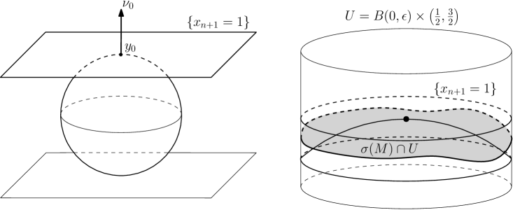
Figure 5. The setting of the proof that $\sigma$ is proper in Proposition 4.15: in the upper half-plane model, the image of $\sigma$ is contained below the horosphere $\{x_{n+1}=1\}$ and in the outer side of the horosphere $x_{1}^{2}+\ldots+x_{n}^{2}+(x_{n+1}-\frac{1}{2})^{2}=\frac{1}{4}$. On the right, the neighbourhood $U$ of $y_{0}$, where the image of $\sigma$ is proved to be the graph of a function $h:B(0,\epsilon)\to{\mathbb{R}}$.

By an application of Lemma 4.11 one can easily show that the Gauss map $G_{\sigma}:M\to\mathcal{G}(\mathbb{H}^{n+1})$ is injective as well if $\sigma$ is complete and has small principal curvatures. However, we will prove here (Proposition 4.16) a stronger property of the Gauss map.

Recall that the space of oriented geodesics of $\mathbb{H}^{n+1}$ has the natural identification

$$\mathcal{G}(\mathbb{H}^{n+1})\cong\partial\mathbb{H}^{n+1}\times\partial\mathbb{H}^{n+1}\setminus\Delta~{},$$

for $\Delta$ the diagonal, given by mapping an oriented geodesic $\ell$ to its endpoints at infinity according to the orientation: as a consequence, the map $G_{\sigma}$ can be seen as a pair of maps with values in the boundary of $\mathbb{H}^{n}$. More precisely, if we denote by $\gamma:{\mathbb{R}}\to\mathbb{H}^{n+1}$ a parameterized geodesic, then the above identification reads:

$$\gamma\mapsto\left(\lim_{t\to+\infty}\gamma(t),\lim_{t\to-\infty}\gamma(t)\right)~{}.$$ (31)

Given an immersion of an oriented manifold $M^{n}$ into $\mathbb{H}^{n+1}$, composing the Gauss map $G_{\sigma}:M\to\mathcal{G}(\mathbb{H}^{n+1})$ with the above map (31) with values in $\partial\mathbb{H}^{n+1}\times\partial\mathbb{H}^{n+1}$ and projecting on each factor, we obtain the so-called hyperbolic Gauss maps $G^{\pm}_{\sigma}:M\to\partial\mathbb{H}^{n+1}$. They are explicitely expressed by

$$G^{\pm}_{\sigma}(p)=\lim_{t\to\pm\infty}\exp_{\sigma(p)}(t\nu(p))\in\partial\mathbb{H}^{n+1}~{}.$$

The following proposition states their injectivity property under the small principal curvatures assumption, which will be applied in Proposition 4.20,

Proposition 4.16.

Let $M^{n}$ be an oriented manifold and $\sigma:M\to\mathbb{H}^{n+1}$ be a complete immersion with small principal curvatures. Then both hyperbolic Gauss maps $G^{\pm}_{\sigma}:M\to\partial\mathbb{H}^{n+1}$ are diffeomorphisms onto their images. In particular, the Gauss map $G_{\sigma}$ is an embedding.

Proof.

Let us first show that $G_{\sigma}^{\pm}$ are local diffeomorphisms. Recalling the definition of $\sigma_{t}$ (Definition 3.4) and its expression in the hyperboloid model of $\mathbb{H}^{n+1}$ (Equation (25)), $G_{\sigma}^{\pm}$ is the limit for $t\to\pm\infty$ in $\partial\mathbb{H}^{n+1}$ of

$$\sigma_{t}(p)=\cosh(t)\sigma(p)\pm\sinh(t)\nu(p)~{}.$$

Recalling the definition of the boundary of $\mathbb{H}^{n+1}$ as the projectivization of the null-cone (Equation (7)), we will consider the boundary at infinity of $\mathbb{H}^{n+1}$ as the slice of the null-cone defined by $\{x_{n+2}=1\}$. Given $p_{0}\in M$, up to isometries we can assume that $\sigma(p_{0})=(0,\ldots,0,1)$ and $\nu(p_{0})=(1,0,\ldots,0)$, so that $G_{\sigma}^{\pm}(p_{0})=(\pm 1,0,\ldots,0,1)$ and the tangent spaces to the image of $\sigma$ at $p_{0}$ and of $\partial\mathbb{H}^{n+1}$ at $G_{\sigma}^{\pm}(p)$ are identified to the same subspace $\{x_{1}=x_{n+2}=0\}$ in ${\mathbb{R}}^{n,1}$.

To compute the differential of $G_{\sigma}^{\pm}$ at $p_{0}$, we must differentiate the maps

$$p\mapsto\lim_{t\to\pm\infty}\frac{\sigma_{t}(p)}{|\langle\sigma_{t}(p),\sigma(p_{0})\rangle|}=\frac{\sigma(p)\pm\nu(p)}{|\langle\sigma(p)\pm\nu(p),\sigma(p_{0})\rangle|}$$

at $p=p_{0}$. Under these identifications, a direct computation for $V\in T_{p_{0}}M$ gives:

$$dG_{\sigma}^{\pm}(V)=d\sigma\circ(\mathrm{id}\mp B)(V)~{}.$$

Hence both differentials of $G_{\sigma}^{\pm}$ are invertible at $p_{0}$ if the eigenvalues of $B$ are always different from $1$ and $-1$, as in our hypothesis. This shows that $G_{\sigma}^{+}$ and $G_{\sigma}^{-}$ are local diffeomorphisms.

To see that $G_{\sigma}^{\pm}$ is injective, suppose that $G_{\sigma}^{\pm}(p)=G_{\sigma}^{\pm}(q)$. This means that $\sigma$ is orthogonal at $p$ and $q$ to two geodesics having a common point at infinity. Hence $\sigma$ is tangent at $p$ and $q$ to two horospheres $H_{p}$ and $H_{q}$ having the same point at infinity. By Lemma 4.11 the image of $\sigma$ must lie in the concave side of both $H_{p}$ and $H_{q}$, hence the two horospheres must coincide. But by Lemma 4.11 again, $\sigma(M\setminus\{p\})$ lies strictly in the concave side of $H_{p}$, hence necessarily $p=q$. See Figure 6.

By the invariance of the domain, $G_{\sigma}^{\pm}$ are diffeomorphisms onto their images. Under the identification between $\mathcal{G}(\mathbb{H}^{n+1})$ and $\partial\mathbb{H}^{n+1}\times\partial\mathbb{H}^{n+1}\setminus\Delta$ the Gauss map $G_{\sigma}$ corresponds to $(G_{\sigma}^{+},G_{\sigma}^{-})$, and it follows that $G_{\sigma}$ is an embedding. ∎

Figure 6. The proof of the injectivity of $G_{\sigma}^{+}$. Suppose two orthogonal geodesics share the final point, hence the image of $\sigma$ is tangent at $\sigma(p)$ and $\sigma(q)$ have the same point at infinity. As a consequence of Lemma 4.11, this is only possible if the two tangent horospheres coincide, and therefore if $p=q$. Replacing horospheres by metric spheres, the same argument proves that the orthogonal geodesics at different points are disjoint (See Proposition 4.18).

4.4. Nearly-Fuchsian manifolds

Taking advantage of the results so far established in this section, we now introduce nearly-Fuchsian representations and manifolds. These will appear again at the end of Section 6 and in Section 7.

Definition 4.17.

Let $M^{n}$ be a closed orientable manifold. A representation $\rho:\pi_{1}(M)\to\mathrm{Isom}^{+}(\mathbb{H}^{n+1})$ is called nearly-Fuchsian if there exists a $\rho$-equivariant immersion $\widetilde{\sigma}:\widetilde{M}\to\mathbb{H}^{n+1}$ with small principal curvatures.

We recall that an immersion $\widetilde{\sigma}\colon\widetilde{M}\to\mathrm{Isom}^{+}(\mathbb{H}^{n+1})$ is $\rho$-equivariant if

$$\widetilde{\sigma}\circ\alpha=\rho(\alpha)\circ\widetilde{\sigma}~{}.$$ (32)

for all $\alpha\in\pi_{1}(M)$. Let us show that the action of nearly-Fuchsian representations is “good” on $\mathbb{H}^{n+1}$ (Proposition 4.18) and also on a region in $\partial\mathbb{H}^{n+1}$ which is the disjoint union of two topological discs (Proposition 4.20).

Proposition 4.18.

Let $M^{n}$ be a closed orientable manifold and $\rho:\pi_{1}(M)\to\mathrm{Isom}^{+}(\mathbb{H}^{n+1})$ be a nearly-Fuchsian representation. Then $\rho$ gives a free and properly discontinous action of $\pi_{1}(M)$ on $\mathbb{H}^{n+1}$. Moreover $\rho$ is convex cocompact, namely there exists a $\rho$-invariant geodesically convex subset $\mathcal{C}\subset\mathbb{H}^{n+1}$ such that the quotient $\faktor{\mathcal{C}}{\rho(\pi_{1}(M))}$ is compact.

Proof.

Let $\widetilde{\sigma}$ be an equivariant immersion as in Definition 4.17. We claim that the family of geodesics orthogonal to $\widetilde{\sigma}(\widetilde{M})$ gives a foliation of $\mathbb{H}^{n+1}$. Observing that the action of $\pi_{1}(M)$ on $\widetilde{M}$ is free and properly discontinous, this immediately implies that the action of $\pi_{1}(M)$ on $\mathbb{H}^{n+1}$ induced by $\rho$ is free and properly discontinous.

By repeating the same argument that shows, in the proof of Proposition 4.16, the injectivity of $G_{\widetilde{\sigma}}^{\pm}$, replacing horospheres with metric spheres of $\mathbb{H}^{n+1}$ and using Remark 4.12, one can prove that two geodesics orthogonal to $\widetilde{\sigma}(\widetilde{M})$ at different points are disjoint.

To show that the orthogonal geodesics give a foliation of $\mathbb{H}^{n+1}$, it remains to show that every point $x\in\mathbb{H}^{n+1}$ is contained in a geodesic of this family (which is necessarily unique). Of course we can assume $x\notin\widetilde{\sigma}(\widetilde{M})$. By cocompactness, $\widetilde{\sigma}$ is complete, hence it is a proper embedding by Proposition 4.15. Then the map that associates to each element of $\widetilde{\sigma}(\widetilde{M})$ its distance from $x$ attains its minimum: this implies that there exists $r>0$ such that the metric sphere of radius $r$ centered at $x$ is tangent to $\widetilde{\sigma}(\widetilde{M})$ at some point $p$. Hence $x$ is on the geodesic through $p$. See Figure 8.

Let us now prove that $\rho$ is also convex-cocompact. To show this, we claim that there exists $t_{+},t_{-}\in{\mathbb{R}}$ such that $\widetilde{\sigma}_{t_{+}}$ is a convex embedding, and $\widetilde{\sigma}_{t_{-}}$ a concave one. Indeed in the proof of Lemma 4.5 we showed that the principal curvatures of the normal evolution $\widetilde{\sigma}_{t}$ are equal to $\tanh(\mu_{i}-t)$, where $\mu_{i}$ is the hyperbolic arctangent of the corresponding principal curvature of $\widetilde{\sigma}$. Hence taking $t\ll 0$ (resp. $t\gg 0$) one can make sure that the principal curvatures of $\widetilde{\sigma}_{t}$ are all negative (resp. positive), hence $\widetilde{\sigma}_{t}$ is convex (resp. concave). The region bounded by the images of $\widetilde{\sigma}_{t_{+}}$ and $\widetilde{\sigma}_{t_{-}}$ is then geodesically convex and diffeomorphic to $\widetilde{M}\times[t_{-},t_{+}]$. Under this diffeomorphism, the action of $\pi_{1}(M)$ corresponds to the action by deck transformations on $\widetilde{M}$ and the trivial action on the second factor. Hence its quotient is compact, being diffeomorphic to $M\times[t_{-},t_{+}]$. ∎

This implies that in dimension three, nearly-Fuchsian manifolds are quasi-Fuchsian.

Remark 4.19.

There is another important consequence of Proposition 4.18. Given $\widetilde{\sigma}$ an equivariant immersion as in Definition 4.17, it follows from the cocompactness of the action of $\rho$ on the geodesically convex region $\mathcal{C}$ that $\widetilde{\sigma}$ is a quasi-isometric embedding in the sense of metric spaces. By cocompactness and Remark 4.3, $\widetilde{M}$ is a complete simply connected Riemannian manifold of negative sectional curvature, hence its visual boundary $\partial\widetilde{M}$ in the sense of Gromov is homeomorphic to $S^{n-1}$. By [BS00, Proposition 6.3], $\widetilde{\sigma}$ extends to a continuous injective map $\partial\widetilde{\sigma}$ from the visual boundary $\partial\widetilde{M}$ of $\widetilde{M}$ to $\partial\mathbb{H}^{n+1}$. By compactness of $\partial\widetilde{M}$, the extension of $\widetilde{\sigma}$ is a homeomorphism onto its image.

Since any two $\rho$-equivariant embeddings $\widetilde{\sigma}_{1},\widetilde{\sigma}_{2}:\widetilde{M}\to\mathbb{H}^{n+1}$ are at bounded distance from each other by cocompactness, the extension $\partial\widetilde{\sigma}$ does not depend on $\widetilde{\sigma}$, but only on the representation $\rho$. In conclusion, the image of $\partial\widetilde{\sigma}$ is a topological $(n-1)$-sphere $\Lambda_{\rho}$ in $\partial\mathbb{H}^{n+1}$, called the limit set of the representation $\rho$. We remark that the limit set is equivalently defined as the set of accumulation points of the orbit of any point with respect to the action of $\rho$ on $\mathbb{H}^{n+1}$. See Figure 7.

Figure 7. A picture of the limit set $\Lambda_{\rho}$, which is a topological $(n-1)$-sphere and disconnects $\partial\mathbb{H}^{n+1}$ in two connected components $\Omega_{+}$ and $\Omega_{-}$, which are homeomorphic to $n$-discs.

The following proposition is well-known. We provide a proof for the sake of completeness.

Proposition 4.20.

Let $M^{n}$ be a closed orientable manifold, $\rho:\pi_{1}(M)\to\mathrm{Isom}^{+}(\mathbb{H}^{n+1})$ be a nearly-Fuchsian representation and $\Lambda_{\rho}$ be its limit set. Then the action of $\rho$ extends to a free and properly discontinous action on $\partial\mathbb{H}^{n+1}\setminus\Lambda_{\rho}$, which is the disjoint union of two topological $n$-discs.

Proof.

Since the action of $\pi_{1}(M)$ on $\widetilde{M}$ is free and properly discontinuous, and $G_{\widetilde{\sigma}}^{\pm}$ are diffeomorphisms onto their image by Proposition 4.16, it follows that the action of $\rho(\pi_{1}(M))$ is free and properly discontinuous on $G_{\widetilde{\sigma}}^{+}(\widetilde{M})$ and $G_{\widetilde{\sigma}}^{-}(\widetilde{M})$, which are topological discs in $\mathbb{H}^{n+1}$ since $\widetilde{M}$ is diffeomorphic to ${\mathbb{R}}^{n}$. We claim that

$$G_{\widetilde{\sigma}}^{+}(\widetilde{M})\cup G_{\widetilde{\sigma}}^{-}(\widetilde{M})=\partial\mathbb{H}^{n+1}\setminus\Lambda_{\rho}~{}.$$

Observe that, by the Jordan-Brouwer separation Theorem, the complement of $\Lambda_{\rho}$ has two connected components, hence the claim will also imply that $G_{\widetilde{\sigma}}^{+}(\widetilde{M})$ and $G_{\widetilde{\sigma}}^{-}(\widetilde{M})$ are disjoint because they are both connected.

In order to show that $\partial\mathbb{H}^{n+1}\setminus\Lambda_{\rho}\subseteq G_{\widetilde{\sigma}}^{+}(\widetilde{M})\cup G_{\widetilde{\sigma}}^{-}(\widetilde{M})$, one can repeat the same argument as Proposition 4.18, now using horospheres, to see that every $x$ in the complement of $\Lambda_{\rho}$ is the endpoint of some geodesic orthogonal to ${\widetilde{\sigma}}(\widetilde{M})$. See Figure 8.

It only remains to show the other inclusion. By continuity, it suffices to show that every $x\in\Lambda_{\rho}$ is not on the image of $G_{\widetilde{\sigma}}^{\pm}$. Observe that by cocompactness the principal curvatures of $\widetilde{\sigma}$ are bounded by some constant $\epsilon<1$ in absolute value. Now, if $x\in\partial\mathbb{H}^{n+1}$ is the endpoint of an orthogonal line $\ell$, then, for all $r$, one would be able to construct a $r$-cap tangent to $\ell\cap\widetilde{\sigma}(\widetilde{M})$ such that $x$ lies in the convex side of the $r$-cap: since, by Remark 4.13, for some $r$ the image of $\widetilde{\sigma}$ lies in the concave side of the $r$-cap, $x$ cannot lie in $\partial\widetilde{\sigma}(\widetilde{M})=\Lambda_{\rho}$. See Figure 8 again. ∎

Figure 8. The arguments in the proof of Proposition 4.20. On the left, since $\widetilde{\sigma}$ is proper and extends to $\Lambda_{\rho}$ in $\partial\mathbb{H}^{n+1}$, from every point $x\notin\Lambda_{\rho}$ one can find a horosphere with point at infinity $x$ tangent to the image of $\widetilde{\sigma}$. The same argument works for an interior point $x$, using metric balls, which is the argument of Proposition 4.18. On the right, a $r$-cap orthogonal to a geodesic $\ell$ with endpoint $x$. Since $\widetilde{\sigma}$ lies on the concave side of tangent $r$-caps for large $r$, $x$ cannot be in the image of $G_{\widetilde{\sigma}}^{\pm}$. The same argument is used in Lemma 7.7, under the convexity assumption, in which case it suffices to use tangent hyperplanes instead of $r$-caps.

As a consequence of Proposition 4.18, if $\rho:\pi_{1}(M)\to\mathrm{Isom}^{+}(\mathbb{H}^{n+1})$ is a nearly-Fuchsian representation, then the quotient $\faktor{\mathbb{H}^{n+1}}{\rho(\pi_{1}(M))}$ is a complete hyperbolic manifold diffeomorphic to $M\times{\mathbb{R}}$. This motivates the following definition.

Definition 4.21.

A hyperbolic manifold of dimension $n+1$ is nearly-Fuchsian if it is isometric to the quotient $\faktor{\mathbb{H}^{n+1}}{\rho(\pi_{1}(M))}$, for $M$ a closed orientable $n$-manifold and $\rho:\pi_{1}(M)\to\mathrm{Isom}^{+}(\mathbb{H}^{n+1})$ a nearly-Fuchsian representation.

Remark 4.22.

If $\widetilde{\sigma}:\widetilde{M}\to\mathbb{H}^{n+1}$ is a $\rho$-equivariant embedding with small principal curvatures, then $\widetilde{\sigma}$ descends to the quotient defining a smooth injective map $\sigma\colon M\to\faktor{\mathbb{H}^{n+1}}{\rho(\pi_{1}(M))}$. Moreover, since $\widetilde{\sigma}$ is a $\rho$-equivariant homeomorphism with its image, $\sigma$ is a homeomorphism with its image as well hence its image is an embedded hypersurface.

We conclude this section with a final definition which appears in the statement of Theorem G. As a preliminary remark, recall from Propositions 4.16 and 4.20 that if $\widetilde{\sigma}$ is a $\rho$-equivariant embedding with small principal curvatures, then each of the Gauss maps $G_{\widetilde{\sigma}}^{\pm}$ of ${\widetilde{\sigma}}$ is a diffeomorphism between $\widetilde{M}$ and a connected component of $\partial\mathbb{H}^{n+1}\setminus\Lambda_{\rho}$. Let us denote these connected components by $\Omega_{\pm}$ as in Figure 7, so that:

$$\partial\mathbb{H}^{n+1}\setminus\Lambda_{\rho}=\Omega_{+}\sqcup\Omega_{-}\qquad G_{\widetilde{\sigma}}^{+}(\widetilde{M})=\Omega_{+}\qquad G_{\widetilde{\sigma}}^{-}(\widetilde{M})=\Omega_{-}~{}.$$

with the representation $\rho$ inducing an action of $\pi_{1}(M)$ on both $\Omega_{+}$ and $\Omega_{-}$. Recalling the identification

$$\mathcal{G}(\mathbb{H}^{n+1})\cong\partial\mathbb{H}^{n+1}\times\partial\mathbb{H}^{n+1}\setminus\Delta~{},$$

given by

$$\gamma\mapsto\left(\lim_{t\to+\infty}\gamma(t),\lim_{t\to-\infty}\gamma(t)\right)~{},$$

the following definition is well-posed.

Definition 4.23.

Given a closed oriented $n$-manifold $M$ and a nearly-Fuchsian representation $\rho:\pi_{1}(M)\to\mathrm{Isom}^{+}(\mathbb{H}^{n+1})$, we define $\mathcal{G}_{\rho}$ the quotient:

$$\faktor{\{\gamma\in\mathcal{G}(\mathbb{H}^{n+1})\,|\,\lim_{t\to+\infty}\gamma(t)\in\Omega_{+}\text{ or }\lim_{t\to-\infty}\gamma(t)\in\Omega_{-}\}}{\rho(\pi_{1}(M))}~{}.$$

Observe that, since the action of $\rho(\pi_{1}(M))$ on $\partial\mathbb{H}^{n+1}$ is free and properly discontinuous on both $\Omega_{+}$ and $\Omega_{-}$, it is also free and properly discontinuous on the region of $\mathcal{G}(\mathbb{H}^{n+1})$ consisting of geodesics having either final point in $\Omega_{+}$ or initial point in $\Omega_{-}$. Moreover, such region is simply connected, because it is the union of $\Omega_{+}\times\partial\mathbb{H}^{n+1}\setminus\Delta$ and $\partial\mathbb{H}^{n+1}\times\Omega_{-}\setminus\Delta$, both of which are simply connected (they retract on $\Omega_{+}\times\{\star\}$ and $\{\star\}\times\Omega_{-}$ respectively) and whose intersection $\Omega_{+}\times\Omega_{-}$ is again simply connected. We conclude that $\mathcal{G}_{\rho}$ is a $2n$-manifold whose fundamental group is isomorphic to $\pi_{1}(M)$, and is endowed with a natural para-Kähler structure induced from that of $\mathcal{G}(\mathbb{H}^{n+1})$ (which is preserved by the action of $\mathrm{Isom}^{+}(\mathbb{H}^{n+1})$).

It is important to stress once more that $\Omega_{+}$ and $\Omega_{-}$ only depend on $\rho$ and not on ${\widetilde{\sigma}}$. We made here a choice in the labelling of $\Omega_{+}$ and $\Omega_{-}$ which only depends on the orientation of $M$. The other choice of labelling would result in a “twin” region, which differs from $\mathcal{G}_{\rho}$ by switching the roles of initial and final endpoints.

A consequence of this construction, which is implicit in the statement of Theorem G, is the following:

Corollary 4.24.

Let $M^{n}$ be a closed orientable manifold, $\rho:\pi_{1}(M)\to\mathrm{Isom}^{+}(\mathbb{H}^{n+1})$ be a nearly-Fuchsian representation and ${\widetilde{\sigma}}:\widetilde{M}\to\mathbb{H}^{n+1}$ be a $\rho$-equivariant embedding of small principal curvatures. For a suitable choice of an orientation on $M$, the Gauss map of $\widetilde{\sigma}$ takes values in $\Omega_{+}\times\Omega_{-}$, and induces an embedding of $M$ in $\mathcal{G}_{\rho}$

Proof.

The only part of the statement which is left to prove is that the induced immersion of $M$ in $\mathcal{G}_{\rho}$ is an embedding, but the proof follows with the same argument as in Remark 4.22. ∎

5. Local and global integrability of immersions into $\mathcal{G}(\mathbb{H}^{n+1})$

In this section we introduce a connection on the principal ${\mathbb{R}}$-bundle $\mathrm{p}$ and relate its curvature with the symplectic geometry of the space of geodesics. As a consequence, we characterize, in terms of the Lagrangian condition, the immersions in the space of geodesics which can be locally seen as Gauss maps of immersions into $\mathbb{H}^{n}$.

5.1. Connection on the ${\mathbb{R}}$-principal bundle

Recall that a connection on a principal $G$-bundle $P$ is a $\mathfrak{g}$-valued 1-form $\omega$ on $P$ such that:

• $\mathrm{Ad}_{g}(R_{g}^{*}\omega)=\omega$;

• for every $\xi\in G$, $\omega(X_{\xi})=\xi$ where $X_{\xi}$ is the vector field associated to $\xi$ by differentiating the action of $G$.

In the special case $G={\mathbb{R}}$ which we consider in this paper, $\omega$ is a real-valued 1-form and the first property simply means that $\omega$ is invariant under the ${\mathbb{R}}$-action.

Let us now introduce the connection that we will concretely use.

Definition 5.1.

We define the connection form on $\mathrm{p}:T^{1}\mathbb{H}^{n}\to\mathcal{G}(\mathbb{H}^{n})$ as

$$\omega(X)=g_{T^{1}\mathbb{H}^{n}}(X,\chi_{(x,v)})$$

for $X\in T_{(x,v)}T^{1}\mathbb{H}^{n}$, where $\chi$ is the infinitesimal generator of the geodesic flow.

The 1-form $\omega$ indeed satisfies the two properties of a connection: the invariance under the ${\mathbb{R}}$-action follows immediately from the invariance of $g_{T^{1}\mathbb{H}^{n}}$ (Lemma 2.3) and of $\chi$ (Equation (14)); the second property follows from Equation (10), namely $\omega(\chi_{(x,v)})=g_{T^{1}\mathbb{H}^{n}}(\chi_{(x,v)},\chi_{(x,v)})=1$.

The connection $\omega$ is defined in such a way that the associated Ehresmann connection, which we recall being a distribution of $T^{1}\mathbb{H}^{n}$ in direct sum with the tangent space of the fibers of $\mathrm{p}$, is simply the distribution orthogonal to $\chi$. Indeed the Ehresmann connection associated to $\omega$ is the kernel of $\omega$. The subspaces in the Ehresmann connections defined by the kernel of $\omega$ are usually called horizontal; we will avoid this term here since it might be confused with the horizontal distribution $\mathcal{H}$ with respect to the other bundle structure of $T^{1}\mathbb{H}^{n}$, namely the unit tangent bundle $\pi:T^{1}\mathbb{H}^{n}\to\mathbb{H}^{n}$.

Now, a connection on a principal $G$-bundle is flat if the Ehresmann distribution is integrable, namely, every point admits a local section tangent to the kernel of $\omega$. We will simply refer to such a section as a flat section. The bundle is a trivial flat principal $G$-bundle if it has a global flat section.

Having introduced the necessary language, the following statement is a direct reformulation of Proposition 3.2.

Proposition 5.2.

Given an oriented manifold $M^{n}$ and an immersion $\sigma:M\to\mathbb{H}^{n+1}$, the $G_{\sigma}$-pull-back of $\mathrm{p}:T^{1}\mathbb{H}^{n+1}\to\mathcal{G}(\mathbb{H}^{n+1})$ is a trivial flat bundle.

Proof.

The lift $\zeta_{\sigma}:M\to T^{1}\mathbb{H}^{n+1}$ is orthogonal to $\chi$ by Proposition 3.2 and therefore induces a global flat section of the pull-back bundle via $G_{\sigma}=\mathrm{p}\circ\zeta_{\sigma}$. ∎

5.2. Curvature of the connection

The purpose of this section is to compute the curvature of the connection $\omega$, which is simply the ${\mathbb{R}}$-valued 2-form $d\omega$. (The general formula for the curvature of a connection on a principal $G$-bundle is $d\omega+\frac{1}{2}\omega\wedge\omega$, but the last term vanishes in our case $G={\mathbb{R}}$.)

Remark 5.3.

It is known that the curvature of $\omega$ is the obstruction to the existence of local flat sections. In particular in the next proposition we will use extensively that, given $X,Y\in\chi_{(x,v)}^{\perp}\subset T_{(x,v)}T^{1}\mathbb{H}^{n+1}$, if there exists an embedding $\zeta:M\to T^{1}\mathbb{H}^{n+1}$ such that $\zeta(p)=(x,v)$, that $X,Y\in d\zeta(T_{p}M)$ and that $d\zeta(T_{p}M)\subset\chi^{\perp}$, then $d\omega(X,Y)=0$.

This can be easily seen by a direct argument: if we now denote by $X$ and $Y$ some extensions tangential to the image of $\zeta$, one has

$$d\omega(X,Y)=\partial_{X}(\omega(Y))-\partial_{Y}(\omega(X))-\omega([X,Y])=0~{},$$

since $\omega(X)=\omega(Y)=0$ by the hypothesis that $X$ and $Y$ are orthogonal to $\chi$, whence $\omega(X)=g_{T^{1}\mathbb{H}^{n}}(X,\chi)=0$, and moreover $\omega([X,Y])=0$ since $[X,Y]$ remains tangential to the image of $\sigma$.

The argument can in fact be reversed to see that $d\omega$ is exactly the obstruction to the existence of a flat section, by the Frobenius theorem.

The following proposition represents an essential step to relate the curvature of $\omega$ and the symplectic geometry of the space of geodesics.

Proposition 5.4.

The following identity holds for the connection form $\omega$ on the principal ${\mathbb{R}}$-bundle $\mathrm{p}:T^{1}\mathbb{H}^{n+1}\to\mathcal{G}(\mathbb{H}^{n+1})$ and the symplectic form $\Omega$ of $\mathcal{G}(\mathbb{H}^{n+1})$:

$$d\omega=\mathrm{p}^{*}\Omega~{}.$$

Proof.

We shall divide the proof in several steps.

First, let us show that $d\omega$ is the pull-back of some 2-form on $\mathcal{G}(\mathbb{H}^{n+1})$. Since $d\omega$ is obviously invariant under the geodesic flow, we only need to show that $d\omega(X,\chi_{(x,v)})=0$ for all $X\in T_{(x,v)}T^{1}\mathbb{H}^{n+1}$. Clearly, it suffices to check this for $X\in\chi^{\perp}$. To apply the exterior derivative formula for $d\omega$, we consider $\chi$ as a globally defined vector field and we shall extend $X$ around $(x,v)$. For this purpose, take a curve $c:(-\epsilon,\epsilon)\to T^{1}\mathbb{H}^{n+1}$ such that $c^{\prime}(0)=X$ and $c^{\prime}(s)$ is tangent to $\chi^{\perp}$ for every $s$. Then define the map $f(s,t)=\varphi_{t}(c(s))$ and observe that $\chi=\partial_{t}f$. We thus set $X=\partial_{s}f$, which is the desired extension along a two-dimensional submanifold. Then we have:

$$d\omega(X,\chi)=\partial_{X}(\omega(\chi))-\partial_{\chi}(\omega(X))-\omega[X,\chi]=0~{},$$

where we have used that $\omega(\chi)\equiv 1$, that $\omega(X)=0$ along the curves $t\mapsto\varphi_{t}(x,v)$ (since the curve $c$ is taken to be in the distribution $\chi^{\perp}$ and the geodesic flow preserves both $\chi$ and its orthogonal complement), and finally that $[X,\chi]=0$ since $\chi=\partial_{t}f$ and $X=\partial_{s}f$ are coordinate vector fields for a submanifold in neighborhood of $(x,v)$.

Having proved this, it is now sufficient to show that $d\omega$ and $\mathrm{p}^{*}\Omega$ agree when restricted to $\chi^{\perp}$. Recall that $\Omega$ is defined as $\mathbbm{G}(\cdot,\mathbbm{J}\cdot)$, where $\mathbbm{G}$ and $\mathbbm{J}$ are the push-forward to $T_{\mathrm{p}(x,v)}\mathcal{G}(\mathbb{H}^{n+1})$, by means of the differential of $\mathrm{p}$, of the metric $g_{T^{1}\mathbb{H}^{n+1}}$ and of the para-complex structure $J$ on $\chi^{\perp}$. Thus we must equivalently show that

$$d\omega(X,Y)=g_{T^{1}\mathbb{H}^{n+1}}(X,JY)\qquad\text{for all }X,Y\in\chi_{(x,v)}^{\perp}~{}.$$ (33)

To see this, take an orthonormal basis $\{w_{1},\ldots,w_{n}\}$ for $v^{\perp}\subset T_{x}\mathbb{H}^{n+1}$, and observe that $\{w_{1}^{\mathcal{H}},\ldots,w_{n}^{\mathcal{H}},w_{1}^{\mathcal{V}},\ldots,w_{n}^{\mathcal{V}}\}$ is a $g_{T^{1}\mathbb{H}^{n+1}}$-orthonormal basis of $\chi^{\perp}$. It is sufficient to check (33) for $X,Y$ distinct elements of this basis. We distinguish several cases.

• First, consider the case $X=w_{i}^{\mathcal{H}}$ and $Y=w_{j}^{\mathcal{H}}$, for $i\neq j$. Then $g_{T^{1}\mathbb{H}^{n+1}}(X,JY)=g_{T^{1}\mathbb{H}^{n+1}}(w_{i}^{\mathcal{H}},w_{j}^{\mathcal{V}})=0$ by Definition 2.2. On the other hand, by Example 3.8, if $\sigma$ is the inclusion of the totally geodesic hyperplane orthogonal to $v$ at $x$, then its lift $\zeta_{\sigma}$ is a submanifold in $T^{1}\mathbb{H}^{n+1}$ orthogonal to $\chi$ at every point and tangent to $X$ and $Y$. Then $d\omega(X,Y)=0$ by Remark 5.3.

• Second, consider $X=w_{i}^{\mathcal{V}}$ and $Y=w_{j}^{\mathcal{V}}$, for $i\neq j$. Then again $g_{T^{1}\mathbb{H}^{n+1}}(X,JY)=g_{T^{1}\mathbb{H}^{n+1}}(w_{i}^{\mathcal{V}},w_{j}^{\mathcal{H}})=0$. Here we can apply Example 3.9 instead, and see that there is a $n$-dimensional sphere in $\mathcal{V}^{0}_{(x,v)}$ orthogonal to the fibers of $\mathrm{p}$ and tangent to $X$ and $Y$, whence $d\omega(X,Y)=0$ by Remark 5.3.

• Third, consider $X=w_{i}^{\mathcal{H}}$ and $Y=w_{j}^{\mathcal{V}}$, for $i\neq j$. Then $g_{T^{1}\mathbb{H}^{n+1}}(X,JY)=g_{T^{1}\mathbb{H}^{n+1}}(w_{i}^{\mathcal{H}},w_{j}^{\mathcal{H}})=0$ since $w_{i}$ and $w_{j}$ are orthogonal. Let us now apply Example 3.10, for instance by taking $Q$ the geodesic going through $x$ with speed $w_{i}$. The normal bundle $\mathrm{N}^{1}Q$ is a submanifold orthogonal to the fibers of $\mathrm{p}$ and tangent to $w_{i}^{\mathcal{H}}$ and $w_{j}^{\mathcal{V}}$. So $d\omega(X,Y)=0$ by the usual argument.

• Finally, we have to deal with the case $X=w_{i}^{\mathcal{H}}$ and $Y=w_{i}^{\mathcal{V}}$. Here $g_{T^{1}\mathbb{H}^{n+1}}(X,JY)=g_{T^{1}\mathbb{H}^{n+1}}(w_{i}^{\mathcal{H}},w_{i}^{\mathcal{H}})=1$. For this computation, we may assume $n=1$, up to restricting to the totally geodesic 2-plane spanned by $v$ and $w$, which is a copy of $\mathbb{H}^{2}$. Hence we will simply denote $w_{i}=w$, and moreover we can assume (up to changing the sign) that $w=x\boxtimes v$, where $\boxtimes$ denotes the Lorentzian cross product in ${\mathbb{R}}^{2,1}$. In other words, $(x,v,w)$ forms an oriented orthonormal triple in ${\mathbb{R}}^{2,1}$.

  Now, let us extend $X$ and $Y$ to globally defined vector fields on $T^{1}\mathbb{H}^{2}$, by means of the assignment $(x,v)\mapsto(x\boxtimes v)^{\mathcal{H}}$ and $(x,v)\mapsto(x\boxtimes v)^{\mathcal{V}}$. By this definition, $X$ and $Y$ are orthogonal to $\chi$; we claim that $[X,Y]=-\chi$. This will conclude the proof, since

  $$d\omega(X,Y)=\partial_{X}(\omega(Y))-\partial_{Y}(\omega(X))-\omega[X,Y]=-\omega[X,Y]=g_{T^{1}\mathbb{H}^{2}}(\chi,\chi)=1~{}.$$

  For the claim about the Lie bracket, let us use the hyperboloid model. Then $X=(x\boxtimes v,0)$ and $Y=(0,x\boxtimes v)$. We can consider $X$ and $Y$ as globally defined (by the same expressions) in the ambient space ${\mathbb{R}}^{2,1}\times{\mathbb{R}}^{2,1}$, so as to compute the Lie bracket in ${\mathbb{R}}^{2,1}\times{\mathbb{R}}^{2,1}$, which will remain tangential to $T^{1}\mathbb{H}^{2}$ since $T^{1}\mathbb{H}^{2}$ is a submanifold. Using the formula $[X,Y]=Jac_{X}Y-Jac_{Y}X$, where $Jac_{X}$ denotes the Jacobian of the vector field thought as a map from ${\mathbb{R}}^{3}$ to ${\mathbb{R}}^{3}$, we obtain

  $$[X,Y]=(x\boxtimes(x\boxtimes v),0)-(0,(x\boxtimes v)\boxtimes v)=-(v,x)=-\chi_{(x,v)}$$

  by the standard properties of the cross-product.

In summary, we have shown that $d\omega$ and $\mathrm{p}^{*}\Omega$ coincide on the basis $\{\chi,w_{1}^{\mathcal{H}},\ldots,w_{n}^{\mathcal{H}},w_{1}^{\mathcal{V}},\ldots,w_{n}^{\mathcal{V}}\}$ of $T_{(x,v)}T^{1}\mathbb{H}^{n+1}$, and therefore the desired identity holds. ∎

We get as an immediate consequence the closedness of the fundamental form $\Omega$, a fact whose proof has been deferred from Section 2.3.

Corollary 5.5.

The fundamental form $\Omega=\mathbbm{G}(\cdot,\mathbbm{J}\cdot)$ is closed.

Proof.

Using Proposition 5.4 we have

$$\mathrm{p}^{*}(d\Omega)=d(\mathrm{p}^{*}\Omega)=d(d\omega)=0~{}.$$

Since $\mathrm{p}$ is surjective, it follows that $d\Omega=0$. ∎

5.3. Lagrangian immersions

We have now all the ingredients to relate the Gauss maps of immersed hypersurfaces in $\mathbb{H}^{n+1}$ with the Lagrangian condition for the symplectic geometry of $\mathcal{G}(\mathbb{H}^{n+1})$.

Corollary 5.6.

Given an oriented manifold $M^{n}$ and an immersion $\sigma:M\to\mathbb{H}^{n+1}$, $\nobreak{G_{\sigma}:M\to\mathcal{G}(\mathbb{H}^{n+1})}$ is a Lagrangian immersion.

Proof.

By Proposition 5.2, the pull-back by $G_{\sigma}$ of the principal ${\mathbb{R}}$-bundle $\mathrm{p}$ is flat because there exists $\widehat{G}_{\sigma}=\zeta_{\sigma}:M\to T^{1}\mathbb{H}^{n+1}$ orthogonal to $\chi$ such that $G_{\sigma}=\mathrm{p}\circ\widehat{G}_{\sigma}$. Hence $(\widehat{G}_{\sigma})^{*}d\omega$ vanishes identically and $\widehat{G}_{\sigma}$ induces a flat section of $G_{\sigma}^{*}\mathrm{p}$. But by Proposition 5.4, $(\widehat{G}_{\sigma})^{*}d\omega=(\widehat{G}_{\sigma})^{*}(\mathrm{p}^{*}\Omega)=(G_{\sigma})^{*}\Omega$, therefore $G_{\sigma}$ is Lagrangian. ∎

Observe that in Corollary 5.6 we only use the flatness property of Proposition 5.2, and not the triviality of the pull-back principal bundle. When $M$ is simply connected, we can partially reverse Corollary 5.6, showing that the Lagrangian condition is essentially the only local obstruction.

Corollary 5.7.

Given an orientable simply connected manifold $M^{n}$ and a Lagrangian immersion $G:M\to\mathcal{G}(\mathbb{H}^{n+1})$, there exists an immersion $\zeta:M\to T^{1}\mathbb{H}^{n+1}$ orthogonal to the fibers of $\mathrm{p}$ such that $G=\mathrm{p}\circ\zeta$. Moreover, if $\pi\circ\zeta:M\to\mathbb{H}^{n+1}$ is an immersion, then $G$ coincides with its Gauss map.

Proof.

Since $G$ is Lagrangian, by Proposition 5.2 the $G$-pull-back bundle of $\mathrm{p}$ is flat, and it is therefore a trivial flat bundle since $M$ is simply connected. Hence it admits a global flat section, which provides the map $\zeta:M\to T^{1}\mathbb{H}^{n+1}$ orthogonal to $\chi$. Assuming moreover that $\sigma:=\pi\circ\zeta$ is an immersion, by Proposition 3.3, $G=\mathrm{p}\circ\zeta$ is the Gauss map of $\sigma$. ∎

Clearly the map $\zeta$ is not uniquely determined, and the different choices differ by the action of $\varphi_{t}$. Lemma 5.8, and the following corollary, show that (by post-composing with $\varphi_{t}$ if necessary) one can always find $\zeta$ such that $\pi\circ\zeta$ is locally an immersion.

Lemma 5.8.

Let $M$ be a $n$-manifold and $\zeta:M\to T^{1}\mathbb{H}^{n+1}$ be an immersion orthogonal to $\chi$. Suppose that the differential of $\pi\circ\zeta$ is singular at $p\in M$. Then there exists $\epsilon>0$ such that the differential of $\pi\circ\varphi_{t}\circ\zeta$ at $p$ is non-singular for all $t\in(-\epsilon,\epsilon)\setminus\{0\}$.

Proof.

Let us denote $\zeta_{t}:=\varphi_{t}\circ\zeta$, $\sigma:=\pi\circ\zeta$, and $\sigma_{t}:=\pi\circ\zeta_{t}$. Assume also $\zeta(p)=(x,v)$. Let $\{V_{1},\ldots,V_{k}\}$ be a basis of the kernel of $d_{p}\sigma$ and let us complete it to a basis $\{V_{1},\ldots,V_{n}\}$ of $T_{p}M$. Hence if we denote $w_{j}:=d_{p}\sigma(V_{j})$ for $j>k$, $\{w_{k+1},\ldots,w_{n}\}$ is a basis of the image of $d_{p}\sigma$. Exactly as in the proof of Proposition 3.3, we have $w_{k+1},\ldots,w_{n}\in v^{\perp}\subset T_{x}\mathbb{H}^{n+1}$. Hence we have:

$$d\zeta(V_{1})=u_{1}^{\mathcal{V}},\ldots,d\zeta(V_{k})=u_{k}^{\mathcal{V}},d\zeta(V_{k+1})=w_{k+1}^{\mathcal{H}}+u_{k+1}^{\mathcal{V}},\ldots,d\zeta(V_{n})=w_{n}^{\mathcal{H}}+u_{n}^{\mathcal{V}}$$

for some $u_{1},\ldots,u_{n}\in v^{\perp}$.

On the one hand, since $\zeta$ is an immersion, $u_{1},\ldots,u_{k}$ are linearly independent. On the other hand, $\zeta$ is orthogonal to $\chi$, hence by Remark 5.3 we have $\zeta^{*}d\omega=0$. Using Equation (33), it follows that:

$$g_{T^{1}\mathbb{H}^{n+1}}(d\zeta(V_{i}),J\circ d\zeta(V_{j}))=0$$

for all $i,j=1,\dots n$. Applying this to any choice of $i\leq k$ and $j>k$, we find $\langle u_{i},w_{j}\rangle=0$. Hence $\{u_{1},\ldots,u_{k},w_{k+1},\ldots,w_{n}\}$ is a basis of $v^{\perp}$.

We are now ready to prove the statement. By Equations (12) and (13), we have

$$d\sigma_{t}(V_{i})=d\pi\circ d\varphi_{t}(u_{i}^{\mathcal{V}})=\sinh(t)u_{i}$$

for $1\leq i\leq k$, while

$$d\sigma_{t}(V_{j})=d\pi\circ d\varphi_{t}(w_{j}^{\mathcal{H}}+u_{j}^{\mathcal{V}})=\cosh(t)w_{j}+\sinh(t)u_{j}$$

for $k+1\leq j\leq n$. The proof will be over if we show that $\{d\sigma(V_{1}),\ldots,d\sigma(V_{n})\}$ are linearly independent for $t\in(-\epsilon,\epsilon)$, $t\neq 0$. In light of the above expressions, dividing by $\sinh(t)$ (which is not zero if $t\neq 0$) or $\cosh(t)$, this is equivalent to showing that

$$\{u_{1},\ldots,u_{k},w_{k+1}+\tanh(t)u_{k+1},\ldots,w_{n}+\tanh(t)u_{n}\}$$

are linearly independent for small $t$. This is true because we have proved above that $\{u_{1},\ldots,u_{k},w_{k+1},\ldots,w_{n}\}$ is a basis, and linear independence is an open condition. ∎

Theorem A.

Let $G\colon M^{n}\to\mathcal{G}(\mathbb{H}^{n+1})$ be an immersion. Then $G$ is Lagrangian if and only if for all $p\in M$ there exists a neighbourhood $U$ of $p$ and an immersion $\sigma\colon U\to\mathbb{H}^{n+1}$ such that $G_{\sigma}=G|_{U}$.

Proof.

The “if” part follows from Corollary 5.6. Conversely, let $U$ be a simply connected neighbourhood of $p$. By Corollary 5.7, there exists an immersion $\zeta\colon U\to T^{1}\mathbb{H}^{n+1}$ orthogonal to the fibers of $\mathrm{p}$ such that $G=\mathrm{p}\circ\zeta$. If the differential of $\pi\circ\zeta$ is non-singular at $p$, then, up to restricting $U$, we can assume $\sigma:=\pi\circ\zeta$ is an immersion of $U$ into $\mathbb{H}^{n+1}$. By the second part of Corollary 5.7, $G|_{U}$ is the Gauss map of $\sigma$. If the differential of $\pi\circ\zeta$ is instead singular at $p$, by Lemma 5.8 it suffices to replace $\zeta$ by $\zeta_{t}$ for small $t$ and we obtain the same conclusion. ∎

Let us now approach the problem of global integrability. We provide an example to show that in general $\pi\circ\varphi_{t}\circ\zeta$ might fail to be globally an immersion for all $t\in{\mathbb{R}}$, as we already mentioned after Proposition 3.3.

Example 5.9.

Let us construct a curve $G:(-T,T)\to\mathcal{G}(\mathbb{H}^{2})$ with the property of being locally integrable but not globally integrable.

Fix $r>0$ and a maximal geodesic $\ell$ in $\mathbb{H}^{2}$. Let us consider a smooth curve $\sigma_{+}\colon(-\varepsilon,T)\to\mathbb{H}^{2}$, for some small enough $\varepsilon$ and big enough $T$, so that:

• $\sigma_{+}$ is an immersion and is parameterized by arclength;

• $(\sigma_{+})|_{(-\varepsilon,\varepsilon)}$ lies on the $r$-cap equidistant from $\ell$, oriented in such a way that the induced unit normal vector field $(\nu_{+})|_{(-\varepsilon,\varepsilon)}$ is directed towards $\ell$;

• $(\sigma_{+})|_{(T_{0},T)}$ lies on the metric circle $\{x\in\mathbb{H}^{2}\,|\,d_{\mathbb{H}^{2}}(x,x_{0})=r\}$ for some $x_{0}\in\mathbb{H}^{2}$ and some $\varepsilon<T_{0}<T$, oriented in such a way that the induced unit normal vector field $(\nu_{+})|_{(T_{0},T)}$ is directed towards $x_{0}$.

Figure 9. On the left, the construction of the curve $\sigma_{+}$, which is an arclenght parameterization of a portion of $r$-cap equidistant from $\ell$ for $s\in(-\varepsilon,\varepsilon)$, and of a circle of radius $r$ for $s\in(T_{0},T)$. On the right, the curve $\sigma_{-}$ whose image is obtained by an order-two elliptic isometry from the image of $\sigma_{+}$.

See Figure 9. By a simple computation, for instance using Equation (29), the curvature of $\sigma_{+}$ equals $\tanh(r)$ on $(-\varepsilon,\varepsilon)$ and $\frac{1}{\tanh(r)}$ on $(T_{0},T)$. Hence by the intermediate value theorem, the image of the curvature function $k\colon(-\varepsilon,T)\to{\mathbb{R}}$ contains the interval $[\tanh(r),\frac{1}{\tanh(r)}]$. An important consequence of this observation is that $(\sigma_{+})_{t}$ fails to be an immersion when $t\geq r$. More precisely, if we denote $\zeta_{\sigma_{+}}$ the lift to $T^{1}\mathbb{H}^{2}$ as usual, using Equation (8) analogously as for Equation (26), we obtain that:

$$d(\pi\circ\varphi_{t}\circ\zeta_{\sigma_{+}})(V)=(\cosh(t)-\sinh(t)k)d\sigma(V)~{}.$$

This shows that the differential of $\pi\circ\varphi_{t}\circ\zeta_{\sigma_{+}}$ at a point $s\in(-\varepsilon,T)$ vanishes if and only if

$$\tanh(t)=\frac{1}{k(s)}~{}.$$ (34)

Since the image of the function $k$ contains the interval $[\tanh(r),\frac{1}{\tanh(r)}]$, if $t\geq r$ then there exists $s$ such that Equation (34) is satisfied and therefore $\pi\circ\varphi_{t}\circ\zeta_{\sigma_{+}}$ is not an immersion at $s$.

Now, let $y_{0}\in\ell$ be the point at distance $r$ from $\sigma_{+}(0)$ and let ${R}_{0}\colon\mathbb{H}^{2}\to\mathbb{H}^{2}$ be the symmetry at $y_{0}$, i.e. ${R}_{0}$ is the isometry of $\mathbb{H}^{2}$ such that ${R}_{0}(y_{0})=y_{0}$ and $d_{y_{0}}{R}_{0}=-\mathrm{id}$. Define $\sigma_{-}\colon(-T,\varepsilon)\to\mathbb{H}^{2}$ as

$$\sigma_{-}(s):={R}_{0}(\sigma_{+}(-s)).$$

As a result, the normal vector field $\nu_{-}$ of $\sigma_{-}$ is such that $dR_{0}({\nu_{+}}(s))={-}{\nu_{-}}(-s)$ and the curvature of $\sigma_{-}$ takes any value in the interval $[-\frac{1}{\tanh(r)},-{\tanh(r)}]$. Hence $(\sigma_{-})_{t}$ fails to be an immersion for $t\leq-r$.

Finally, consider the two lifts $\zeta_{\sigma_{+}}$ and $\zeta_{\sigma_{-}}$ in $T^{1}\mathbb{H}^{2}$. By construction one has that for all $s\in(-\varepsilon,\varepsilon)$

$$\varphi_{r}\circ\zeta_{\sigma_{+}}(s)=\varphi_{-r}\circ\zeta_{\sigma_{-}}(s).$$

As a result, we can define our counterexample $\zeta\colon(-T,T)\to T^{1}\mathbb{H}^{2}$ as

$$\zeta(s)=\begin{cases}\varphi_{r}\circ\zeta_{\sigma_{+}}(s)\quad&\text{ if $s>-\varepsilon$}\\ \varphi_{-r}\circ\zeta_{\sigma_{-}}(s)\quad&\text{ if $s<\varepsilon$}\end{cases}.$$

By construction, we have that $\mathrm{p}\circ\zeta_{\sigma_{+}}=\mathrm{p}\circ\zeta|_{(-\varepsilon,T)}$ and $\mathrm{p}\circ\zeta_{\sigma_{-}}=\mathrm{p}\circ\zeta|_{(-T,\varepsilon)}$, therefore $\mathrm{p}\circ\zeta$ is an immersion into $\mathcal{G}(\mathbb{H}^{2})$ and clearly it is locally integrable. However, by the above discussion, $\pi\circ\varphi_{t}\circ\zeta$ fails to be an immersion for every $t\in{\mathbb{R}}$: for $t\geq 0$ because $\pi\circ\varphi_{t}\circ\zeta_{\sigma_{+}}$ has vanishing differential at some $s\geq-\varepsilon$, and for $t\leq 0$ because the differential of $\pi\circ\varphi_{t}\circ\zeta_{\sigma_{-}}$ vanishes at some $s\leq\varepsilon$. See Figure 10.

Figure 10. The curve $\zeta:(-T,T)\to T^{1}\mathbb{H}^{2}$ projects to a map $\pi\circ\zeta$ into $\mathbb{H}^{2}$ which is not an immersion, because it is constantly equal to $x_{0}$ for $s\in(T_{0},T)$ and to $R_{0}(x_{0})$ for $s\in(-T,-T_{0})$. Moreover the curvature of the regular part takes all the values in $(-\infty,+\infty)$. For this reason, each immersion $\varphi_{t}\circ\zeta$ into $T^{1}\mathbb{H}^{2}$ does not project to an immersion in $\mathbb{H}^{2}$.

Corollary 5.7 and Theorem A can be improved under the additional assumption that the immersion $G$ is Riemannian. More precisely, we provide an improved characterization of immersions into $\mathcal{G}(\mathbb{H}^{n+1})$ that are Gauss maps of immersions with small principal curvatures in terms of the Lagrangian and Riemannian condition, again for when $M$ is simply connected.

Theorem B.

Given a simply connected manifold $M^{n}$ and an immersion $G:M^{n}\to\mathcal{G}(\mathbb{H}^{n+1})$, $G$ is Riemannian and Lagrangian if and only if there exists an immersion $\sigma\colon M\to\mathbb{H}^{n+1}$ with small principal curvatures such that $G_{\sigma}=G$.

If in addition $\sigma$ is complete, then it is a proper embedding, $G_{\sigma}$ is an embedding and $M$ is diffeomorphic to ${\mathbb{R}}^{n}$.

Proof.

We know from Corollary 5.6 and Proposition 4.2 that the Riemannian and Lagrangian conditions on $G$ are necessary. To see that they are also sufficient, by Corollary 5.7 there exists $\zeta\colon M\to\mathcal{G}(\mathbb{H}^{n+1})$ orthogonal to the fibers of $\mathrm{p}$ such that $\mathrm{p}\circ\zeta=G$. We claim that $\pi\circ\zeta$ is an immersion, which implies that $G=G_{\sigma}$ for $\sigma=\pi\circ\zeta$ by the second part of Corollary 5.7. Indeed, if $X\in T_{p}M$ is such that $d\zeta(X)\in\mathcal{V}_{\zeta(x)}=\ker(d\pi_{\zeta(x)})$, then $d\zeta(X)=w^{\mathcal{V}}$ for some $w\in T_{\sigma(p)}\mathbb{H}^{n+1}$. Hence by Definition 2.2 and the construction of the metric $\mathbbm{G}$, $\mathbbm{G}(X,X)=-\langle w,w\rangle\leq 0$: since $\mathbbm{G}$ is Riemannian, necessarily $w=0$ and therefore $X=0$.

By Proposition 4.2 $\sigma$ has small principal curvatures. The “in addition” part follows by Proposition 4.15 and Proposition 4.16. ∎

As another consequence of Proposition 4.15 and Proposition 4.16, we obtain the following result.

Theorem C.

Let $M^{n}$ be a manifold. If $G\colon M\to\mathcal{G}(\mathbb{H}^{n+1})$ is a complete Riemannian and Lagrangian immersion, then $M$ is diffeomorphic to ${\mathbb{R}}^{n}$ and there exists a proper embedding $\sigma:M\to\mathbb{H}^{n+1}$ with small principal curvatures such that $G=G_{\sigma}$.

Proof.

Let us lift $G$ to the universal cover $\widetilde{M}$, obtaining a Riemannian and Lagrangian immersion $\widetilde{G}:\widetilde{M}\to\mathcal{G}(\mathbb{H}^{n+1})$ which is still complete. By Theorem B, $\widetilde{G}$ is the Gauss map of an immersion $\sigma$ with small principal curvatures. We claim that $\sigma$ is complete. Indeed by Equation (24) the first fundamental form of $\widetilde{G}$, which is complete by hypothesis, equals $\mathrm{I}-\mathrm{I}\mathrm{I}\mathrm{I}$, hence it is complete since $\mathrm{I}\mathrm{I}\mathrm{I}$ is positive semi-definite.

It follows from Proposition 4.16 that $\widetilde{G}$ is injective. Hence $\widetilde{M}=M$ and $\widetilde{G}=G$, and therefore $G$ is the Gauss map of $\sigma$, which is complete. By the “in addition” part of Theorem B, $\sigma$ is properly embedded and $M$ is diffeomorphic to ${\mathbb{R}}^{n}$. ∎

In summary, the Lagrangian condition is essentially the only local obstruction to realizing an immersion $G:M\to\mathcal{G}(\mathbb{H}^{n+1})$ as the Gauss map of an immersion into $\mathbb{H}^{n+1}$, up to the subtlety that this might be an immersion only when lifted to $T^{1}\mathbb{H}^{n+1}$. This subtlety however never occurs in the small principal curvatures case. In the remainder of the paper, we will discuss the problem of characterizing immersions into $\mathcal{G}(\mathbb{H}^{n+1})$ which are Gauss maps of equivariant immersions into $\mathbb{H}^{n+1}$ with small principal curvatures.

6. Equivariant integrability: the Maslov class

In this section, we provide the first characterization of equivariant immersions in $\mathcal{G}(\mathbb{H}^{n+1})$ which arise as the Gauss maps of equivariant immersions in $\mathbb{H}^{n+1}$, in the Riemannian case. This is the content of Theorem D. We first try to motivate the problem, introduce the obstruction, namely the Maslov class, and study some of its properties. See for instance [Ars00] for a discussion on the Maslov class in more general settings.

6.1. Motivating examples

Given an $n$-manifold $M$, a representation $\rho:\pi_{1}(M)\to\mathrm{Isom}^{+}(\mathbb{H}^{n+1})$, and a $\rho$-equivariant immersion $\widetilde{\sigma}:\widetilde{M}\to\mathbb{H}^{n+1}$, it is immediate to see that the Gauss map $G_{\widetilde{\sigma}}:\widetilde{M}\to\mathcal{G}(\mathbb{H}^{n+1})$ is $\rho$-equivariant (recall also Remark 2.6). Moreover, if ${\widetilde{\sigma}}$ has small principal curvatures, it follows from the discussion of the previous sections that $G_{\widetilde{\sigma}}$ is a Lagrangian and Riemannian immersion.

However, a $\rho$-equivariant Lagrangian immersion (even with the additional assumptions of being Riemannian and being an embedding) does not always arise as the Gauss map associated to a $\rho$-equivariant immersion in $\mathbb{H}^{n+1}$, as the following simple example shows for $n=1$.

Example 6.1.

Let us construct a coordinate system for a portion of $\mathcal{G}(\mathbb{H}^{2})$. Let $\gamma:{\mathbb{R}}\to\mathbb{H}^{2}$ be a geodesic parameterized by arclength, and let us define a map $\Psi:{\mathbb{R}}\times(0,\pi)\to\mathcal{G}(\mathbb{H}^{2})$ by defining $\Psi(t,\theta)$ as the oriented geodesic that intersects $\gamma$ at $\gamma(t)$ with an angle $\theta$ (measured counterclockwise with respect to the standard orientation of $\mathbb{H}^{2}$). We can lift $\Psi$ to a map $\widehat{\Psi}:{\mathbb{R}}\times(0,\pi)\to T^{1}\mathbb{H}^{2}$, which will however not be orthogonal to the fibers of the projection $T^{1}\mathbb{H}^{2}\to\mathcal{G}(\mathbb{H}^{2})$. The lift is simply defined as

$$\widehat{\Psi}(t,\theta)=(\gamma(t),\cos(\theta)\gamma^{\prime}(t)+\sin(\theta)w)~{},$$

where $w$ is the vector forming an angle $\frac{\pi}{2}$ with $\gamma^{\prime}(t)$. We omitted the dependence of $w$ on $t$ since, in the hyperboloid model, $w$ is actually a constant vector in ${\mathbb{R}}^{2,1}$.

Let us compute the pull-back of the metric $\mathbbm{G}$ on $\mathcal{G}(\mathbb{H}^{2})$ by the map $\Psi$. We have already observed in Example 3.9 that the restriction of $\mathbbm{G}$ on the image of $\theta\mapsto\Psi(t_{0},\theta)$ is minus the standard metric of $\mathbb{S}^{1}$. Indeed in this simple case, $d\widehat{\Psi}_{(t,\theta)}(\partial_{\theta})=(0,w)$ is in the vertical subspace $\mathcal{V}^{0}$ and by Definition 2.2 its squared norm is $-1$. On the other hand, since the vector field $\cos(\theta)\gamma^{\prime}(t)+\sin(\theta)w$ is parallel along $\gamma$, when we differentiate in $t$ we obtain, by applying the definition of horizontal lift:

$$d\widehat{\Psi}_{(t,\theta)}(\partial_{t})=\cos(\theta)(\gamma^{\prime}(t))^{\mathcal{H}}+\sin(\theta)w^{\mathcal{H}}~{}.$$ (35)

Moreover, Equation (35) gives the decomposition of $d\widehat{\Psi}_{(t,\theta)}(\partial_{t})$ in $T_{\widehat{\Psi}_{(t,\theta)}}T^{1}\mathbb{H}^{2}={\mathrm{Span}(\chi)\oplus\chi^{\perp}}$ as in Equation (9), since the first term is a multiple of the generator of the geodesic flow, and the second term is in $\mathcal{H}^{0}$. This shows, by definition of the metric $\mathbbm{G}$, that $d\Psi_{(t,\theta)}(\partial_{t})$ has squared norm $\sin^{2}(\theta)$ and that $d\Psi_{(t,\theta)}(\partial_{t})$ and $d\Psi_{(t,\theta)}(\partial_{\theta})$ are orthogonal. In conclusion, we have showed:

$$\Psi^{*}\mathbbm{G}=-d\theta^{2}+\sin^{2}(\theta)dt^{2}~{}.$$

We are now ready to produce our example of $\rho$-equivariant embedding $G:\widetilde{M}\to\mathcal{G}(\mathbb{H}^{2})$ which is not $\rho$-integrable. Consider $M=\mathbb{S}^{1}$, $\widetilde{M}={\mathbb{R}}$, and the representation $\rho:{\mathbb{Z}}\to\mathrm{Isom}^{+}(\mathbb{H}^{2})$ which is a hyperbolic translation along $\gamma$. The induced action on $\mathcal{G}(\mathbb{H}^{2})$ preserves the image of $\Psi$ and its generator acts on the $(t,\theta)$-coordinates simply by $(t,\theta)\mapsto(t+c,\theta)$. Hence the map

$$G:{\mathbb{R}}\to\mathcal{G}(\mathbb{H}^{2})\qquad G(s)=\Psi(s,\theta_{0})$$

for some constant $\theta_{0}\in(0,\pi)$ is a $\rho$-equivariant Riemannian embedding by the above expression of $\Psi^{*}\mathbbm{G}$. Of course the Lagrangian condition is trivially satisfied since $n=1$. By Theorem B $G$ coincides with the Gauss map $G_{\sigma}$ associated to some embedding $\sigma:{\mathbb{R}}\to\mathbb{H}^{2}$ with small curvature. It is easy to see that any such embedding $\sigma$ is not $\rho$-equivariant unless $\theta_{0}=\frac{\pi}{2}$, see Figure 11.

Figure 11. On the left, the family of geodesics forming a fixed angle $\theta$ with the horizontal geodesic (in the Poincaré disc model of $\mathbb{H}^{2}$). On the right, the metric $-d\theta^{2}+\sin^{2}(\theta)dt^{2}$ represents a portion of the Anti-de Sitter space of dimension 2. Here are pictured some lines defined by $\theta=c$, in the projective model of the Anti-de Sitter space.

We also briefly provide an example of a locally integrable, but not globally integrable immersion in $\mathcal{G}(\mathbb{H}^{3})$ for $M$ not simply connected (lifting to the universal cover $\widetilde{M}$ this corresponds to $\rho$ being the trivial representation). This example in particular motivates Corollary E, which is a direct consequence of Theorem D.

Example 6.2.

First, let us consider a totally geodesic plane $\mathcal{P}$ in $\mathbb{H}^{3}$ and an annulus $\mathcal{A}$ contained in $\mathcal{P}$. Let $c:\widetilde{\mathcal{A}}\to\mathcal{A}$ be the universal covering. Then $c$ is an immersion in $\mathbb{H}^{3}$ with small principal curvatures (in fact, totally geodesic), and is clearly not injective. See Figure 12 on the left. Of course, in light of Proposition 4.15, this is possible because the immersion $c$ is not complete.

Now, let us deform $\mathcal{A}$ in the following way. We cut $\mathcal{A}$ along a geodesic segment $s\subset\mathcal{P}$ to obtain a rectangle $\mathcal{R}$ having two (opposite) geodesic sides, say $r_{1}$ and $r_{2}$. Then we deform such rectangle to get an immersion $c^{\prime}:\mathcal{R}\to\mathbb{H}^{3}$, so that one geodesic side remains unchanged (say $c^{\prime}(r_{1})=s$), while the other side $r_{2}$ is mapped to an $r$-cap equidistant from $\mathcal{P}$, for small $r$, in such a way that it projects to $s$ under the normal evolution. We can also arrange $c$ so that a neighbourhood of $r_{1}$ is mapped to $\mathcal{P}$, while a neighbourhood of $r_{2}$ is mapped to the $r$-cap equidistant from $\mathcal{P}$. See Figure 12 on the right.

By virtue of this construction, the Gauss map of $c^{\prime}$ coincides on the edges $r_{1}$ and $r_{2}$ of $\mathcal{R}$, and therefore induces an immersion $G^{\prime}:\mathcal{A}\to\mathcal{G}(\mathbb{H}^{3})$. Clearly $G^{\prime}$ is locally integrable, but not globally integrable. In other words, the lift to the universal cover of $G^{\prime}$ is a $\rho$-equivariant immersion of $\widetilde{A}$ to $\mathcal{G}(\mathbb{H}^{3})$ which is not $\rho$-integrable, for $\rho$ the trivial representation.

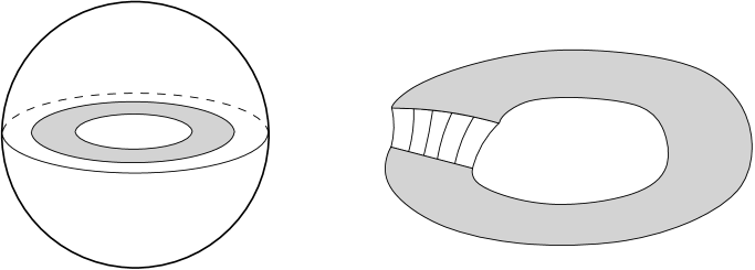
Figure 12. On the left, a totally geodesic annulus $\mathcal{A}$ in a plane $\mathcal{P}$. On the right, an embedded rectangle with the property that a neighbourhood of one side lies in $\mathcal{P}$, while a neighbourhood of the opposite side lies on an $r$-cap equidistant from $\mathcal{P}$. Such rectangle induces an embedding of $\mathcal{A}$ in $\mathcal{G}(\mathbb{H}^{3})$ which is locally, but not globally, integrable.

Motivated by the previous examples, we introduce the relevant definition for our problem.

Definition 6.3.

Given an $n$-manifold $M$ and a representation $\rho\colon\pi_{1}(M)\to\mathrm{Isom}^{+}(\mathbb{H}^{n+1})$, a $\rho$-equivariant immersion $G\colon\widetilde{M}\to\mathcal{G}(\mathbb{H}^{n+1})$ is $\rho$-integrable if there exists a $\rho$-equivariant immersion ${\widetilde{\sigma}}\colon\widetilde{M}\to\mathbb{H}^{n+1}$ whose Gauss map is $G$.

6.2. Maslov class

Let us now introduce the obstruction which will permit us to classify $\rho$-integrable Lagrangian immersions under the Riemannian assumption, namely the Maslov class. For this purpose, let $G:\widetilde{M}\to\mathcal{G}(\mathbb{H}^{n+1})$ be a Riemannian immersion. The second fundamental form of $G$ is a symmetric bilinear form on $M$ with values in the normal bundle of $G$, defined as

$$\overline{\mathrm{I}}\mathrm{I}(V,W)=({\mathbbm{D}}_{G_{*}V}(G_{*}W))^{\perp}$$

for vector fields $V,W$, where $\mathbbm{D}$ denotes the ambient Levi-Civita connection of $\mathbbm{G}$ and $\perp$ the projection to the normal subspace of $G$. One can prove that $\overline{\mathrm{I}}\mathrm{I}(V,W)$ is a tensor, i.e. that it depends on the value of $V$ and $W$ pointwise. The mean curvature is then

$$\overline{\mathrm{H}}=\frac{1}{n}\mathrm{tr}_{\overline{\mathrm{I}}}\overline{\mathrm{I}}\mathrm{I}~{},$$

that is, it is the trace of $\overline{\mathrm{I}}\mathrm{I}$ with respect to the first fundamental form $\overline{\mathrm{I}}$ of $G$, and is therefore a section of the normal bundle of $G$.

Consider now the 1-form on $\widetilde{M}$ given by $G^{*}(\Omega(\overline{\mathrm{H}},\cdot))$. It will follow from Proposition 6.5 (see Corollary 6.7) that this is a closed 1-form. Since $\mathrm{Isom}^{+}(\mathbb{H}^{n+1})$ acts by automorphisms of the para-Kähler manifold $(\mathcal{G}(\mathbb{H}^{n+1}),\mathbbm{G},\mathbb{J},\Omega)$, if $G$ is $\rho$-equivariant, then the form $G^{*}(\Omega(\overline{\mathrm{H}},\cdot))$ is $\pi_{1}(M)$-invariant: as a result, it defines a well-posed closed 1-form on $M$. Its cohomology class is the so-called Maslov class:

Definition 6.4.

Given an $n$-manifold $M$, a representation $\rho\colon\pi_{1}(M)\to\mathrm{Isom}^{+}(\mathbb{H}^{n+1})$ and a $\rho$-equivariant Lagrangian and Riemannian immersion $G\colon\widetilde{M}\to\mathcal{G}(\mathbb{H}^{n+1})$, the Maslov class of $G$ is the cohomology class

$$\mu_{G}:=[G^{*}(\Omega(\overline{\mathrm{H}},\cdot))]\in H_{dR}^{1}(M)~{}.$$

The main result of this section is the following, and it will be deduced as a consequence of Theorem 6.12.

Theorem D.

Given an orientable $n$-manifold $M$ and a representation $\rho\colon\pi_{1}(M)\to\mathrm{Isom}^{+}(\mathbb{H}^{n+1})$, a $\rho$-equivariant Riemannian and Lagrangian immersion $G\colon\widetilde{M}\to\mathcal{G}(\mathbb{H}^{n+1})$ is $\rho$-integrable if and only if $\mu_{G}=0$ in $H_{dR}^{1}(M)$.

We immediately obtain the following characterization of global integrability for $\pi_{1}(M)\neq\{1\}$.

Corollary E.

Given an orientable $n$-manifold $M$ and an immersion $G\colon M\to\mathcal{G}(\mathbb{H}^{n+1})$, $G$ is the Gauss map of an immersion $\sigma:M\to\mathbb{H}^{n+1}$ of small principal curvatures if and only if $G$ is Riemannian and Lagrangian and $\mu_{G}=0$ in $H_{dR}^{1}(M)$.

Proof.

Denote $\rho$ the trivial representation. Given $G:M\to\mathcal{G}(\mathbb{H}^{n+1})$, precomposing with the universal covering map we obtain an immersion $\widetilde{G}:\widetilde{M}\to\mathcal{G}(\mathbb{H}^{n+1})$ which is $\rho$-equivariant. Observe that $\widetilde{G}$ is the Gauss map of some immersion $\widetilde{\sigma}:\widetilde{M}\to\mathbb{H}^{n+1}$ by Theorem B. Then $G$ is the Gauss map of some immersion in $\mathbb{H}^{n+1}$ if and only if $\widetilde{\sigma}$ descends to the quotient $M$, i.e. it is $\rho$-integrable. Hence this is equivalent to the vanishing of the Maslov class by Theorem D. ∎

6.3. Mean curvature of Gauss maps

Recall that, given an embedding $\sigma:M\to\mathbb{H}^{n+1}$ with small principal curvatures, we introduced in (27) the function $f_{\sigma}:M\to{\mathbb{R}}$ which is the mean of the hyperbolic arctangents of the principal curvatures of $\sigma$. This function is strictly related to the mean curvature of the Gauss map of $\sigma$, as in the following proposition.

Proposition 6.5.

Let $M^{n}$ be an oriented manifold, $\sigma:M\to\mathbb{H}^{n+1}$ an embedding with small principal curvatures, and $G_{\sigma}:M\to\mathcal{G}(\mathbb{H}^{n+1})$ its Gauss map. Then

$$G_{\sigma}^{*}(\Omega(\overline{\mathrm{H}},\cdot))=d(f_{\sigma})=d\left({\frac{1}{n}}\sum_{i=1}^{n}\mathrm{arctanh}\lambda_{i}\right)~{},$$

where $\lambda_{1},\ldots,\lambda_{n}$ denote the principal curvatures of $\sigma$.

The essential step in the proof of Proposition 6.5 is the following computation for the mean curvature vector of the Gauss map $G_{\sigma}$:

$$\overline{\mathrm{H}}=-\mathbbm{J}(dG_{\sigma}(\overline{\nabla}f_{\sigma}))~{},$$ (36)

where $\overline{\nabla}$ denotes the gradient with respect to the first fundamental form $\overline{\mathrm{I}}$ of $G_{\sigma}$. Indeed, once Equation (36) is established, Proposition 6.5 follows immediately since

$$\Omega(\overline{\mathrm{H}},dG_{\sigma}(V))=-\mathbbm{G}(\mathbbm{J}(\overline{\mathrm{H}}),dG_{\sigma}(V))=\mathbbm{G}(dG_{\sigma}(\overline{\nabla}f_{\sigma}),dG_{\sigma}(V))=df_{\sigma}(V)~{}.$$

The computations leading to Equation (36) will be done in $T^{1}\mathbb{H}^{n+1}$ equipped with the metric $\widehat{g}_{T^{1}\mathbb{H}^{n+1}}$ defined in Remark 2.8, which is the restriction of the flat pseudo-Riemannian metric (20) of ${\mathbb{R}}^{n+1,1}\times{\mathbb{R}}^{n+1,1}$ to $T^{1}\mathbb{H}^{n+1}$, seen as a submanifold as in (5). This approach is actually very useful: the Levi-Civita connection of $\widehat{g}_{T^{1}\mathbb{H}^{n+1}}$ on $T^{1}\mathbb{H}^{n+1}$, that we denote by $\widehat{D}$, will be just the normal projection of the flat connection $\mathrm{d}$ of ${\mathbb{R}}^{n+1,1}\times{\mathbb{R}}^{n+1,1}$ to $T^{1}\mathbb{H}^{n+1}$.

Indeed, the following lemma will be useful to compute the Levi-Civita connection $\mathbbm{D}$ of $\mathcal{G}(\mathbb{H}^{n+1})$. Given a vector $X\in T_{\ell}\mathcal{G}(\mathbb{H}^{n+1})$ and $(x,v)\in\mathrm{p}^{-1}(\ell)$, we define the horizontal lift of $X$ at $(x,v)$ as the unique vector $\widetilde{X}\in T_{(x,v)}T^{1}\mathbb{H}^{n+1}$ such that

$$\widetilde{X}\in\chi_{(x,v)}^{\perp}\qquad\text{and}\qquad d\mathrm{p}(\widetilde{X})=X~{}.$$ (37)

For a vector field $X$ on an open set $U$ of $\mathcal{G}(\mathbb{H}^{n+1})$, we will also refer to the vector field $\widetilde{X}$ on $\mathrm{p}^{-1}(U)$, defined by the conditions (37), as the horizontal lift of the vector field $X$.

Lemma 6.6.

Given two vector fields $X,Y$ on $\mathbbm{G}$,

$$\mathbbm{D}_{X}Y=d\mathrm{p}(\widehat{D}_{\widetilde{X}}\widetilde{Y})$$

Proof.

By the well-known characterization of the Levi-Civita connection, it is sufficient to prove that the expression $\mathbbm{A}_{X}Y:=d\mathrm{p}(\widehat{D}_{\widetilde{X}}\widetilde{Y})$ is a well-posed linear connection which is torsion-free and compatible with the metric of $\mathbbm{G}$. We remark that this is not obvious because, although the metric of $\mathbbm{G}$ is the restriction of the metric $\widehat{g}_{T^{1}\mathbb{H}^{n+1}}$ to $\chi^{\perp}$, there is no flat section of the bundle projection $p:T^{1}\mathbb{H}^{n+1}\to\mathcal{G}(\mathbb{H}^{n+1})$, hence $\mathcal{G}(\mathbb{H}^{n+1})$ cannot be seen as an isometrically embedded submanifold of $T^{1}\mathbb{H}^{n+1}$.

First, observe that the expression $(\mathbbm{A}_{X}Y)_{|\ell}=(d_{(x,v)}\mathrm{p})(\widehat{D}_{\widetilde{X}}\widetilde{Y})$ does not depend on the choice of the point $(x,v)\in\mathrm{p}^{-1}(\ell)$. Indeed, given two points $(x_{1},v_{1})$ and $(x_{2},v_{2})$ in $\mathrm{p}^{-1}(\ell)$, there exists $t$ such that $(x_{2},v_{2})=\varphi_{t}(x_{1},v_{1})$. By a small adaptation of Lemma 2.3, the geodesic flow $\varphi_{t}$ acts by isometries of the metric $\widehat{g}_{T^{1}\mathbb{H}^{n+1}}$ (see also Remarks 2.7 and 2.8), hence it also preserves the horizontal lifts $\widetilde{X}$ and $\widetilde{Y}$ and the Levi-Civita connection $\widehat{D}$. Hence $d\mathrm{p}(\widehat{D}_{\widetilde{X}}\widetilde{Y})=\mathbbm{A}_{X}Y$ is a well-defined vector field on $\mathcal{G}(\mathbb{H}^{n+1})$ whose horizontal lift is the projection of $\widehat{D}_{\widetilde{X}}\widetilde{Y}$ to $\chi^{\bot}$.

We check that $\mathbbm{A}$ is a linear connection. It is immediate to check the additivity in $X$ and $Y$. Moreover we have the $C^{\infty}$-linearity in $X$ since:

$$\mathbbm{A}_{fX}Y=d\mathrm{p}\left(\widehat{D}_{(f\circ\mathrm{p})\widetilde{X}}\widetilde{Y}\right)=d\mathrm{p}\left((f\circ\mathrm{p})\hat{D}_{\widetilde{X}}\widetilde{Y}\right)=f(\mathbbm{A}_{X}Y)~{},$$

and the Leibnitz rule in $Y$, for:

$$\mathbbm{A}_{X}(fY)=d\mathrm{p}\left(\partial_{\widetilde{X}}(f\circ\mathrm{p})\ \widetilde{Y}+(f\circ\mathrm{p})\widehat{D}_{\widetilde{X}}\widetilde{Y}\right)=\partial_{X}f\ Y+f(\mathbbm{A}_{X}Y)~{}.$$

The connection $\mathbbm{A}$ is torsion-free:

$$\mathbbm{A}_{X}Y-\mathbbm{A}_{Y}X=d\mathrm{p}(\widehat{D}_{\widetilde{X}}\widetilde{Y})-d\mathrm{p}(\widehat{D}_{\widetilde{Y}}\widetilde{X})=d\mathrm{p}([\widetilde{X},\widetilde{Y}])=[X,Y]~{}.$$

Finally, we show that $\mathbbm{A}$ is compatible with the metric $\mathbbm{G}$:

$$\mathbbm{G}(\mathbbm{A}_{X}Y,Z)+\mathbbm{G}(Y,\mathbbm{A}_{X}Z) =\widehat{g}_{T^{1}\mathbb{H}^{n+1}}(\widetilde{\mathbbm{A}_{X}Y},\widetilde{Z})+\widehat{g}_{T^{1}\mathbb{H}^{n+1}}(\widetilde{Y},\widetilde{\mathbbm{A}_{X}Z})=$$

$$=\widehat{g}_{T^{1}\mathbb{H}^{n+1}}(\widehat{D}_{\widetilde{X}}\widetilde{Y},\widetilde{Z})+\widehat{g}_{T^{1}\mathbb{H}^{n+1}}(\widetilde{Y},\widehat{D}_{\widetilde{X}}\widetilde{Z})=$$

$$=\partial_{\widetilde{X}}(\widehat{g}_{T^{1}\mathbb{H}^{n+1}}(\widetilde{Y},\widetilde{Z}))=\partial_{X}(\mathbbm{G}(Y,Z))~{},$$

where in the first line we used the definition of $\mathbbm{G}$, and in the second line the fact that the horizontal lift of $\mathbbm{A}_{X}Y$ is the orthogonal projection (with kernel spanned by $\chi$) of $\widehat{D}_{\widetilde{X}}\widetilde{Y}$. ∎

We are now ready to provide the proof of Proposition 6.5.

Proof of Proposition 6.5.

As already observed after Equation (36), it suffices to prove that $\overline{\mathrm{H}}=-\mathbbm{J}(dG_{\sigma}(\overline{\nabla}f_{\sigma}))$. So we shall compute the mean curvature vector of $G_{\sigma}$ in $\mathcal{G}(\mathbb{H}^{n+1})$. For this purpose, let $\{e_{1},\ldots,e_{n}\}$ be a local frame on $M$ which is orthonormal with respect to the first fundamental form $\overline{\mathrm{I}}=G_{\sigma}^{*}\mathbbm{G}$. To simplify the notation, let us denote $\epsilon_{i}:=dG_{\sigma}(e_{i})$. Then $\{\mathbbm{J}\epsilon_{1},\ldots,\mathbbm{J}\epsilon_{n}\}$ is an orthonormal basis for the normal bundle of $G_{\sigma}$, on which the metric $\mathbbm{G}$ is negative definite since $G_{\sigma}$ is Riemannian. The mean curvature vector can be computed as:

$$\overline{\mathrm{H}}=\frac{1}{n}\sum_{i=1}^{n}\overline{\mathrm{I}}\mathrm{I}(\epsilon_{i},\epsilon_{i})=-\frac{1}{n}\sum_{i=1}^{n}\sum_{k=1}^{n}\mathbbm{G}(\overline{\mathrm{I}}\mathrm{I}(\epsilon_{i},\epsilon_{i}),\mathbbm{J}\epsilon_{k})\mathbbm{J}\epsilon_{k}=-\frac{1}{n}\sum_{i=1}^{n}\sum_{k=1}^{n}\mathbbm{G}(\mathbbm{D}_{\epsilon_{i}}\epsilon_{i},\mathbbm{J}\epsilon_{k})\mathbbm{J}\epsilon_{k}~{},$$

where in the last equality we used that $\overline{\mathrm{I}}\mathrm{I}(V,W)$ is the normal projection of $\mathbbm{D}_{V}W$.

Let us now apply this expression to a particular $\overline{\mathrm{I}}$-orthonormal frame $\{e_{1},\ldots,e_{n}\}$ obtained in the following way. Pick a local $\mathrm{I}$-orthogonal frame on $M$ of eigenvectors for the shape operator $B$ of $\sigma$, and normalize each of them so as to have unit norm for $\overline{\mathrm{I}}$. Hence each $e_{i}$ is an eigenvector of $B$, whose corresponding eigenvalue $\lambda_{i}$ are the principal curvatures of $\sigma$. We claim that, with this choice, $\mathbbm{G}(\mathbbm{D}_{\epsilon_{i}}\epsilon_{i},\mathbbm{J}\epsilon_{k})=d(\mathrm{arctanh}\lambda_{i})(e_{k})$. This will conclude the proof, for

$$\overline{\mathrm{H}}=\frac{1}{n}\mathbbm{J}\left(\sum_{i=1}^{n}\sum_{k=1}^{n}d(\mathrm{arctanh}\lambda_{i})(e_{k})\epsilon_{k}\right)=\mathbbm{J}\left(\sum_{k=1}^{n}\partial_{e_{k}}f_{\sigma}\ dG_{\sigma}(e_{k})\right)=\mathbbm{J}(dG_{\sigma}(\overline{\nabla}f_{\sigma})))~{}.$$

To show the claim, we will first use Lemma 6.6 to get

$$\mathbbm{G}(\mathbbm{D}_{\epsilon_{i}}\epsilon_{i},\mathbbm{J}\epsilon_{k})=\widehat{g}_{T^{1}\mathbb{H}^{n+1}}(\widehat{D}_{\widetilde{\epsilon}_{i}}\widetilde{\epsilon}_{i},J\widetilde{\epsilon}_{k})~{},$$

where $\widehat{D}$ is the Levi-Civita connection of $\widehat{g}_{T^{1}\mathbb{H}^{n+1}}$ and $\widetilde{\epsilon}_{i}$ is the horizontal lift of $\epsilon_{i}$. As in Equation (22), we can write

$$d\zeta_{\sigma}(e_{i})=(d\sigma(e_{i}),-\lambda_{i}d\sigma(e_{i}))$$

and the Levi-Civita connection $\widehat{D}$ is the normal projection with respect to the metric (20) of the flat connection $\mathrm{d}$ of ${\mathbb{R}}^{n+1,1}\times{\mathbb{R}}^{n+1,1}$. Hence we can compute:

$$\mathbbm{G}(\mathbbm{D}_{\epsilon_{i}}\epsilon_{i},\mathbbm{J}\epsilon_{k}) =-\lambda_{k}\langle\mathrm{d}_{d\sigma(e_{i})}d\sigma(e_{i}),d\sigma(e_{k})\rangle+\lambda_{i}\langle\mathrm{d}_{d\sigma(e_{i})}d\sigma(e_{i}),d\sigma(e_{k})\rangle+\partial_{e_{i}}\lambda_{i}\langle d\sigma(e_{i}),d\sigma(e_{k})\rangle$$

$$=(\lambda_{i}-\lambda_{k})\ \mathrm{I}(\nabla_{e_{i}}e_{i},e_{k})+(\partial_{e_{i}}\lambda_{i})\ \mathrm{I}(e_{i},e_{k})~{}.$$

We recall that $g$ denotes the first fundamental form of $\sigma$, and $\nabla$ its Levi-Civita connection, and in the last equality we used that the Levi-Civita connection of $\mathbb{H}^{n+1}$ is the projection to the hyperboloid in Minkowski space ${\mathbb{R}}^{n+1,1}$ of the ambient flat connection.

Now, when $i=k$ we obtained the desired result:

$$\mathbbm{G}(\mathbbm{D}_{\epsilon_{i}}\epsilon_{i},\mathbbm{J}\epsilon_{i})=\frac{\partial_{e_{i}}\lambda_{i}}{1-\lambda_{i}^{2}}=d(\mathrm{arctanh}\lambda_{i})(e_{i})$$

since $e_{i}$ is a unit vector for the metric $\overline{\mathrm{I}}$, hence using the expression $\overline{\mathrm{I}}=\mathrm{I}-\mathrm{I}\mathrm{I}\mathrm{I}$ from Equation (24) its squared norm for the metric $\mathrm{I}$ is $(1-\lambda_{i}^{2})^{-1}$. When $i\neq k$, the latter term disappears since $\{e_{1},\ldots,e_{n}\}$ is an orthogonal frame for $g$, and we are thus left with showing that

$$(\lambda_{i}-\lambda_{k})\ \mathrm{I}(\nabla_{e_{i}}e_{i},e_{k})=d(\mathrm{arctanh}\lambda_{i})(e_{k})~{}.$$

For this purpose, using the compatibility of $\nabla$ with the metric, namely $\partial_{e_{i}}(\mathrm{I}(e_{i},e_{k}))=\mathrm{I}(\nabla_{e_{i}}e_{i},e_{k})+\mathrm{I}(e_{i},\nabla_{e_{i}}e_{k})$, that $\mathrm{I}(e_{i},e_{k})=0$, and that $\nabla$ is torsion-free, we get:

$$(\lambda_{i}-\lambda_{k})\ \mathrm{I}(\nabla_{e_{i}}e_{i},e_{k})=-(\lambda_{i}-\lambda_{k})\ \mathrm{I}(e_{i},\nabla_{e_{i}}e_{k})=\lambda_{k}\ \mathrm{I}(e_{i},\nabla_{e_{i}}e_{k})-\lambda_{i}\ \mathrm{I}(e_{i},\nabla_{e_{k}}e_{i})-\lambda_{i}\ \mathrm{I}(e_{i},[e_{i},e_{k}])~{}.$$

Now, recall that the Codazzi equation for $\sigma$ is $d^{\nabla}B=0$. Applying it to the vector fields $e_{i}$ and $e_{k}$, we obtain

$$d^{\nabla}B(e_{i},e_{k})=\nabla_{e_{i}}(\lambda_{k}e_{k})-\nabla_{e_{k}}(\lambda_{i}e_{i})-B([e_{i},e_{k}])=0,$$

from which we derive

$$\lambda_{k}\nabla_{e_{i}}e_{k}-\lambda_{i}\nabla_{e_{k}}e_{i}=(\partial_{e_{k}}\lambda_{i})e_{i}-(\partial_{e_{i}}\lambda_{k})e_{k}+B([e_{i},e_{k}])~{}.$$ (38)

Using Equation (38) in the previous expression, we finally obtain:

$$(\lambda_{i}-\lambda_{k})\ \mathrm{I}(\nabla_{e_{i}}e_{i},e_{k})= (\partial_{e_{k}}\lambda_{i})\ \mathrm{I}(e_{i},e_{i})-(\partial_{e_{i}}\lambda_{k})\ \mathrm{I}(e_{i},e_{k})+\mathrm{I}(e_{i},B[e_{i},e_{k}])-\mathrm{I}(B(e_{i}),[e_{i},e_{k}])$$

$$= \frac{\partial_{e_{k}}\lambda_{i}}{1-\lambda_{i}^{2}}=d(\mathrm{arctanh}\lambda_{i})(e_{k})$$

where the cancellations from the first to the second line are due to the fact that $B$ is $\mathrm{I}$-self adjoint and that $\mathrm{I}(e_{i},e_{k})=0$. This concludes the proof. ∎

Corollary 6.7.

Given an $n$-manifold $M$, a representation $\rho\colon\pi_{1}(M)\to\mathrm{Isom}^{+}(\mathbb{H}^{n+1})$ and a $\rho$-equivariant Lagrangian and Riemannian immersion $G\colon\widetilde{M}\to\mathcal{G}(\mathbb{H}^{n+1})$, the Maslov class $\mu_{G}$ is a well-defined cohomology class in $H^{1}_{dR}(M,{\mathbb{R}})$.

Proof.

By Theorem B, $G$ is the Gauss map of a (in general non equivariant) immersion $\sigma:\widetilde{M}\to\mathbb{H}^{n+1}$. By Proposition 6.5, the 1-form $G^{*}(\Omega(\overline{\mathrm{H}},\cdot))$ on $\widetilde{M}$ is exact, and $\rho$-equivariant, hence it induces a closed 1-form on $M$ whose cohomology class is $\mu_{G}$ as in Definition 6.4. ∎

6.4. Holonomy of flat principal bundles

An immediate consequence of Proposition 6.5 is that the vanishing of the Maslov class is a necessary condition for a $\rho$-equivariant Lagrangian and Riemannian embedding $G:\widetilde{M}\to\mathcal{G}(\mathbb{H}^{n+1})$ to be $\rho$-integrable (Definition 6.3). Indeed, if $\widetilde{\sigma}:\widetilde{M}\to\mathbb{H}^{n+1}$ is a $\rho$-equivariant embedding with $G_{\widetilde{\sigma}}=G$ (hence necessarily with small principal curvatures), then the function $f_{\widetilde{\sigma}}$ descends to a well-defined function on $M$, hence by Proposition 6.5 $G^{*}(\Omega(\overline{\mathrm{H}},\cdot))$ is an exact 1-form, i.e. the Maslov class $\mu_{G_{\widetilde{\sigma}}}$ vanishes. We will now see that this condition is also sufficient, which will be a consequence of a more general result, Theorem 6.12.

Let $G:\widetilde{M}\to\mathcal{G}(\mathbb{H}^{n+1})$ be a $\rho$-equivariant Lagrangian and Riemannian embedding. We have already used that the $G$-pull-back bundle $\widetilde{\mathrm{p}}_{G}\colon\widetilde{P}\to\widetilde{M}$ of $\mathrm{p}:T^{1}\mathbb{H}^{n+1}\to\mathcal{G}(\mathbb{H}^{n+1})$ is a flat trivial ${\mathbb{R}}$-principal bundle over $\widetilde{M}$, namely, it is isomorphic, as a flat principal bundle, to the trivial bundle $\widetilde{M}\times{\mathbb{R}}\to\widetilde{M}$ with flat sections $\widetilde{M}\times\{\ast\}$. Moreover, $G$ being $\rho$-equivariant, the fundamental group $\pi_{1}(M)$ acts freely and properly discontinously on $\widetilde{P}$, thus inducing a flat ${\mathbb{R}}$-principal bundle structure $\mathrm{p}_{G}\colon P\to M$, where $P$ is the quotient of $\widetilde{P}$ by the action of $\pi_{1}(M)$. However the bundle $\mathrm{p}_{G}\colon P\to M$ is not trivial in general. The obstruction to triviality is represented by the holonomy of the bundle, which can be defined, in our setting, as follows.

Definition 6.8.

Let $P\to M$ be a flat principal ${\mathbb{R}}$-bundle that is isomorphic to the quotient of the trivial bundle $\widetilde{M}\times{\mathbb{R}}\to\widetilde{M}$ by an equivariant (left) action of $\pi_{1}(M)$. The holonomy representation is the representation $\mathrm{hol}:\pi_{1}(M)\to{\mathbb{R}}$ such that the action of $\pi_{1}(M)$ is expressed by:

$$\alpha\cdot(m,s)=(\alpha\cdot m,\mathrm{hol}(\alpha)+s)~{}.$$

Remark 6.9.

Fix $p\in M$ and $\alpha$ a closed $C^{1}$ loop based at $p$. Then pick a horizontal lift $\widehat{\alpha}$ to the total space of $\mathrm{p}_{G}$, namely with $\frac{d\widehat{\alpha}}{dt}$ orthogonal to the fibers, so that $\mathrm{p}\circ\widehat{\alpha}=\alpha$. (The lift is uniquely determined by its initial point in $\mathrm{p}_{G}^{-1}(p)$.) It follows from Definition 6.8 that

$$\mathrm{hol}_{G}(\alpha)\cdot\widehat{\alpha}(1)=\widehat{\alpha}(0).$$

In the identification $\pi_{1}(M)=\pi_{1}(M,[p])$, this allows to give an alternative definition of $\mathrm{hol}_{G}$ through homotopy classes of closed paths in $M$.

Remark 6.10.

We remark that in general, for flat principal $G$-bundles, the holonomy representation is only defined up to conjugacy, but in out case $G={\mathbb{R}}$ is abelian and therefore $\mathrm{hol}$ is uniquely determined by the isomorphism class of the flat principal bundle.

Also observe that, since ${\mathbb{R}}$ is abelian, $\mathrm{hol}_{G}$ induces a map from $H_{1}(M,{\mathbb{Z}})$ to ${\mathbb{R}}$, where $H_{1}(M,{\mathbb{Z}})$ is the first homology group of $M$ and we are using that there is a canonical isomorphism between $H_{1}(M,{\mathbb{Z}})$ and the abelianization of the fundamental group of $M$ in a point. Equivalently, $\mathrm{hol}_{G}$ is identified to an element of $H^{1}(M,{\mathbb{R}})$.

We can interpret the holonomy of the principal bundle $\mathrm{p}_{G}$ in terms of the geometry of $\mathbb{H}^{n+1}$. Global flat sections of the trivial bundle $\widetilde{\mathrm{p}}_{G}\colon\widetilde{P}\to\widetilde{M}$ correspond to Riemannian embeddings $\zeta:\widetilde{M}\to T^{1}\mathbb{H}^{n+1}$ as in Corollaries 5.6 and 5.7. By Theorem B, such a $\zeta$ is the lift to $T^{1}\mathbb{H}^{n+1}$ of an embedding $\sigma:\widetilde{M}\to\mathbb{H}^{n+1}$ with small principal curvatures.

Now, let $\alpha\in\pi_{1}(M)$. By equivariance of $G$, namely $G\circ\alpha=\rho(\alpha)\circ G$, it follows that $\mathrm{p}\circ\zeta\circ\alpha=\mathrm{p}\circ\rho(\alpha)\circ\zeta$, hence $\rho(\alpha)\circ\zeta\circ\alpha^{-1}:\widetilde{M}\to T^{1}\mathbb{H}^{n+1}$ provides another flat section of the pull-back bundle $\widetilde{\mathrm{p}}_{G}$. Therefore there exists $t_{\alpha}\in{\mathbb{R}}$ such that

$$\varphi_{t_{\alpha}}\circ\zeta=\rho(\alpha)\circ\zeta\circ\alpha^{-1}~{}.$$ (39)

Then the value $t_{\alpha}$ is precisely the holonomy of the quotient bundle $\mathrm{p}_{G}$, namely the group representation

$$\mathrm{hol}_{G}\colon\pi_{1}(M)\to{\mathbb{R}}\qquad\mathrm{hol}_{G}(\alpha)=t_{\alpha}$$

A direct consequence of this discussion is the following:

Lemma 6.11.

Given an $n$-manifold $M$ and a representation $\rho\colon\pi_{1}(M)\to\mathrm{Isom}^{+}(\mathbb{H}^{n+1})$, a $\rho$-equivariant Lagrangian and Riemannian embedding $G\colon\widetilde{M}\to\mathcal{G}(\mathbb{H}^{n+1})$ is $\rho$-integrable if and only if the ${\mathbb{R}}$-principal flat bundle $\mathrm{p}_{G}$ is trivial.

Proof.

The bundle $\mathrm{p}_{G}$ is trivial if and only if its holonomy $\mathrm{hol}_{G}$ vanishes identically, that is, if and only if $t_{\alpha}=0$ for every $\alpha\in\pi_{1}(M)$. By the above construction, this is equivalent to the condition that $\zeta\circ\alpha=\rho(\alpha)\circ\zeta$ for all $\alpha$, which is equivalent to $\sigma\circ\alpha=\rho(\alpha)\circ\sigma$, namely that $\sigma$ is $\rho$-equivariant. ∎

We are ready to prove the following.

Theorem 6.12.

Given an $n$-manifold $M$, a representation $\rho\colon\pi_{1}(M)\to\mathrm{Isom}^{+}(\mathbb{H}^{n+1})$ and a $\rho$-equivariant Lagrangian and Riemannian embedding $G\colon\widetilde{M}\to\mathcal{G}(\mathbb{H}^{n+1})$, the holonomy of $\mathrm{p}_{G}$ is given by

$$\mathrm{hol}_{G}(\alpha)=\int_{\alpha}\mu_{G}.$$

for all $\alpha\in\pi_{1}(M)$.

Observe that Theorem D follows immediately from Theorem 6.12 since, by the standard de Rham Theorem, there exists an isomorphism

$$\begin{split}H_{dR}^{1}(M,{\mathbb{R}})&\xrightarrow{\sim}H^{1}(M,{\mathbb{R}})\\ \eta&\mapsto\bigg{(}\xi\mapsto\int_{\xi}\eta\bigg{)},\end{split}$$

hence $\mathrm{hol}_{G}\equiv 0$ if and only if $\mu_{G}=0$.

Proof of Theorem 6.12.

Let $\zeta:\widetilde{M}\to T^{1}\mathbb{H}^{n+1}$ be a map such that $\mathrm{p}\circ\zeta=G$, so as to induce a global section of the pull-back bundle $\widetilde{\mathrm{p}}_{G}$. Then by Equation (39) the holonomy $t_{\alpha}=\mathrm{hol}_{G}(\alpha)$ satisfies $\varphi_{t_{\alpha}}\circ\zeta\circ\alpha=\rho(\alpha)\circ\zeta$. By Proposition 3.5, this gives the following equivariance relation for $\sigma=\pi\circ\zeta$:

$$(\sigma\circ\alpha)_{t_{\alpha}}=\rho(\alpha)\circ\sigma~{}.$$

Let now $f_{\sigma}$ denote the mean of the hyperbolic arctangents of the principal curvatures, as in Equation (27). Lemma 4.5 and the fact that $\rho(\alpha)$ acts isometrically imply:

$$f_{\sigma\circ\alpha}=f_{\sigma}+t_{\alpha}~{}.$$

Now, by Proposition 6.5 and the definition of the Maslov class, we have:

$$\int_{\alpha}\mu_{G}=\int_{\alpha}df_{\sigma}=f_{\sigma}(\alpha(p))-f_{\sigma}(p)=t_{\alpha}$$

for any point $p\in M$. This concludes the proof. ∎

6.5. Minimal Lagrangian immersions

We prove here two direct corollaries of Theorem D. Let us first recall the definition of minimal Lagrangian (Riemannian) immersions.

Definition 6.13.

A Riemannian immersion of an $n$-manifold into $\mathcal{G}(\mathbb{H}^{n+1})$ is minimal Lagrangian if:

• its mean curvature vector vanishes identically;

• it is Lagrangian with respect to the symplectic form $\Omega$.

Our first corollary is essentially a consequence of Theorem D.

Corollary 6.14.

Let $M^{n}$ be a closed orientable manifold and $\rho:\pi_{1}(M)\to\mathrm{Isom}^{+}(\mathbb{H}^{n+1})$ a representation. If $G:\widetilde{M}\to\mathcal{G}(\mathbb{H}^{n+1})$ is a $\rho$-equivariant Riemannian minimal Lagrangian immersion, then $G$ is the Gauss map of a $\rho$-equivariant embedding $\widetilde{\sigma}:\widetilde{M}\to\mathbb{H}^{n+1}$ with small principal curvatures such that

$$f_{\widetilde{\sigma}}={\frac{1}{n}}\sum_{i=1}^{n}\mathrm{arctanh}\lambda_{i}=0~{}.$$

In particular, $\rho$ is a nearly-Fuchsian representation and $G$ is an embedding.

We remark that if $n=2$, then the condition $f_{\widetilde{\sigma}}=0$ is equivalent to $\lambda_{1}+\lambda_{2}=0$ since $\mathrm{arctanh}$ is an odd and injective function. That is, in this case $\widetilde{\sigma}$ is a minimal embedding in $\mathbb{H}^{3}$.

Proof.

Suppose $G$ is a $\rho$-equivariant minimal Lagrangian immersion. Since its mean curvature vector vanishes identically, we have $\mu_{G}=0$ and therefore $G$ is $\rho$-integrable by Theorem D. That is, there exists a $\rho$-equivariant immersion $\widetilde{\sigma}:\widetilde{M}\to\mathbb{H}^{n+1}$ such that $G=G_{\widetilde{\sigma}}$. By Proposition 4.2, $\widetilde{\sigma}$ has small principal curvatures, hence $\rho$ is nearly-Fuchsian. By Proposition 6.5, we have that $f_{\widetilde{\sigma}}$ is constant. By Lemma 4.5, up to taking the normal evolution, we can find $\widetilde{\sigma}$ such that $f_{\widetilde{\sigma}}$ vanishes identically.

Finally, $\widetilde{\sigma}$ is complete by cocompactness, and therefore both $\widetilde{\sigma}$ and $G$ are embeddings by Proposition 4.15 and Proposition 4.16. ∎

The following is a uniqueness result for $\rho$-equivariant minimal Lagrangian immersions.

Corollary F.

Given a closed orientable manifold $M^{n}$ and a representation $\rho:\pi_{1}(M)\to\mathrm{Isom}^{+}(\mathbb{H}^{n+1})$, there exists at most one $\rho$-equivariant Riemannian minimal Lagrangian immersion $G:\widetilde{M}\to\mathcal{G}(\mathbb{H}^{n+1})$ up to reparametrization. If such a $G$ exists, then $\rho$ is nearly-Fuchsian and $G$ induces a minimal Lagrangian embedding of $M$ in $\mathcal{G}_{\rho}$.

Proof.

Suppose that $G$ and $G^{\prime}$ are $\rho$-equivariant minimal Lagrangian immersions. By Corollary 6.14, there exist $\rho$-equivariant embeddings $\widetilde{\sigma},\widetilde{\sigma}^{\prime}:\widetilde{M}\to\mathbb{H}^{n+1}$ with small principal curvatures such that $G=G_{\widetilde{\sigma}}$ and $G^{\prime}=G_{\widetilde{\sigma}^{\prime}}$, with $f_{\widetilde{\sigma}}=f_{\widetilde{\sigma}^{\prime}}=0$. Moreover, $G$ and $G^{\prime}$ induce embeddings in $\mathcal{G}_{\rho}$ by Corollary 4.24.

By Remark 4.22, both $\sigma$ and $\sigma^{\prime}$ induce embeddings of $M$ in the nearly-Fuchsian manifold $\faktor{\mathbb{H}^{n+1}}{\rho(\pi_{1}(M))}$; let us denote with $\Sigma$ and $\Sigma^{\prime}$ the corresponding images. We claim that $\Sigma=\Sigma^{\prime}$, which implies the uniqueness in the statement.

To see this, consider the signed distance from $\Sigma$, which is a proper function

$$r:\faktor{\mathbb{H}^{n+1}}{\rho(\pi_{1}(M))}\to{\mathbb{R}}~{}.$$

Since $\Sigma^{\prime}$ is closed, $r|_{\Sigma^{\prime}}$ admits a maximum value $r_{\max}$ achieved at some point $x_{\max}\in\Sigma^{\prime}$. This means that at the point $x_{\max}$, $\Sigma^{\prime}$ is tangent to a hypersurface $\Sigma_{r_{\max}}$ at signed distance $r_{\max}$ from $\Sigma$, and $\Sigma^{\prime}$ is contained in the side of $\Sigma_{r_{\max}}$ where $r$ is decreasing. This implies that, if $B^{\prime}$ denotes the shape operator of $\Sigma^{\prime}$ and $B_{r_{\max}}$ that of $\Sigma_{r_{\max}}$, both computed with respect to the unit normal vector pointing to the side of increasing $r$, then $B_{r_{\max}}-B^{\prime}$ is positive semi-definite at $x_{\max}$.

Let us now denote by $\lambda_{1},\ldots,\lambda_{n}$ the eigenvalues of $B_{r_{\max}}$ and $\lambda^{\prime}_{1},\ldots,\lambda_{n}^{\prime}$ those of $B^{\prime}$. Let us moreover assume that $\lambda_{1}\leq\ldots\leq\lambda_{n}$ and similarly for the $\lambda_{i}^{\prime}$. By Weyl’s monotonicity theorem, $\lambda_{i}\geq\lambda_{i}^{\prime}$ at $x_{\max}$ for $i=1,\ldots,n$. Since $\mathrm{arctanh}$ is a monotone increasing function, this implies that

$$\sum_{i=1}^{n}\mathrm{arctanh}\lambda_{i}(x_{\max})\geq\sum_{i=1}^{n}\mathrm{arctanh}\lambda_{i}^{\prime}(x_{\max})~{}.$$

Since $f_{\widetilde{\sigma}^{\prime}}=0$, the right-hand side vanishes. On the other hand, since $f_{\widetilde{\sigma}}=0$, from Lemma 4.5 the left-hand side is identically equal to $-r_{\max}$. Hence $r_{\max}\leq 0$. Repeating the same argument replacing the maximum point of $r$ on $\Sigma^{\prime}$ by the minimum point, one shows $r_{\min}\geq 0$. Hence $r|_{\Sigma^{\prime}}$ vanishes identically, which proves that $\Sigma=\Sigma^{\prime}$ and thus concludes the proof. ∎

7. Equivariant integrability: Hamiltonian symplectomorphisms

In this section we will provide the second characterization of $\rho$-integrability, in the case of a nearly-Fuchsian representation $\rho:\pi_{1}(M)\to\mathrm{Isom}^{+}(\mathbb{H}^{n+1})$. We first introduce the terminology and state the result (Theorem G); then we introduce the so-called Lagrangian Flux map which will play a central role in the proof of Theorem G.

7.1. Hamiltonian group and nearly-Fuchsian manifolds

We will restrict hereafter to the case of nearly-Fuchsian representations $\rho:\pi_{1}(M)\to\mathrm{Isom}^{+}(\mathbb{H}^{n+1})$. Let $G:\widetilde{M}\to\mathcal{G}(\mathbb{H}^{n+1})$ be a $\rho$-integrable immersion as in Definition 6.3. Since $\rho$ is nearly-Fuchsian, we showed in Corollary 4.24 that $G$ induces an embedded submanifold in the para-Kähler manifold $\mathcal{G}_{\rho}$, defined in Definition 4.23. This motivates the following definition in the spirit of Definition 6.3.

Definition 7.1.

Given a closed orientable $n$-manifold $M$ and a nearly-Fuchsian representation $\rho:\pi_{1}(M)\to\mathrm{Isom}^{+}(\mathbb{H}^{n+1})$, an embedding $M\to\mathcal{G}_{\rho}$ is $\rho$-integrable if it is induced in the quotient from a $\rho$-integrable embedding ${G}\colon\widetilde{M}\to\mathcal{G}(\mathbb{H}^{n+1})$. Similarly, an embedded submanifold $\mathcal{L}\subset\mathcal{G}_{\rho}$ is $\rho$-integrable if it is the image of a $\rho$-integrable embedding.

Theorem G below gives a description of the set of $\rho$-integrable submanifolds $\mathcal{L}\subset\mathcal{G}_{\rho}$ which are induced by immersions $G$ with small principal curvatures. Clearly, as we have previously shown, a necessary condition on $\mathcal{L}$ is that of being Lagrangian and Riemannian. To state the theorem, we need to recall the notion of Hamiltonian symplectomorphism.

Definition 7.2.

Given a symplectic manifold $(\mathcal{X},\Omega)$, a compactly supported symplectomorphism $\Phi$ is Hamiltonian if there exists a compactly supported smooth function $F_{\bullet}:\mathcal{X}\times[0,1]\to{\mathbb{R}}$ such that $\Phi=\Phi_{1}$, where $\Phi_{s_{0}}$ is the flow at time $s_{0}$ of the (time-dependent) vector field $X_{s}$ defined by:

$$dF_{s}=\Omega(X_{s},\cdot)~{}.$$ (40)

The isotopy $\Phi_{\bullet}:\mathcal{X}\times[0,1]\to\mathcal{X}$ is called Hamiltonian isotopy.

Remark 7.3.

If $\Phi_{\bullet}$ is a Hamiltonian isotopy as in Definition 7.2, then $\Phi_{s}$ is a symplectomorphism for every $s\in[0,1]$. Indeed

$$\mathcal{L}_{X_{s}}\Omega=\iota_{X_{s}}d\Omega+d(\iota_{X_{s}}\Omega)=0$$

as a consequence of Cartan’s formula and Equation (40), and $\Phi_{s}$ is clearly Hamiltonian.

Compactly supported Hamiltonian symplectomorphisms form a group which we will denote by $\mathrm{Ham}_{c}(\mathcal{X},\Omega)$.

The aim of this section is to prove the following result.

Theorem G.

Let $M$ be a closed orientable $n$-manifold, $\rho:\pi_{1}(M)\to\mathrm{Isom}^{+}(\mathbb{H}^{n+1})$ be a nearly-Fuchsian representation and $\mathcal{L}\subset\mathcal{G}_{\rho}$ a Riemannian $\rho$-integrable submanifold. Then a Riemannian submanifold $\mathcal{L}^{\prime}$ is $\rho$-integrable if and only if there exists $\Phi\in\mathrm{Ham}_{c}(\mathcal{G}_{\rho},\Omega)$ such that $\Phi(\mathcal{L})=\mathcal{L}^{\prime}$.

Of course, although not stated in Theorem G, both $\mathcal{L}$ and $\mathcal{L}^{\prime}$ are necessarily Lagrangian as a consequence of Corollary 5.6.

7.2. The Lagrangian Flux

We shall now define the Flux map for Lagrangian submanifolds, which was introduced in [Sol13], and relate it to the holonomy of ${\mathbb{R}}$-principal bundles.

Definition 7.4.

Let $(\mathcal{X},\Omega)$ be a symplectic manifold and let $\Upsilon_{\bullet}:M\times[0,1]\to\mathcal{X}$ be a smooth map such that each $\Upsilon_{t}$ is a Lagrangian embedding of $M$. Then we define:

$$\mathrm{Flux}(\Upsilon_{\bullet})=\int_{0}^{1}\Upsilon_{s}^{*}(\Omega(X_{s},\cdot))ds\in H^{1}_{dR}(M,{\mathbb{R}})~{},$$

where

$$X_{s_{0}}(\Upsilon_{s_{0}}(p))=\left.\frac{d}{ds}\right|_{s=s_{0}}\Upsilon_{s}(p)\in T_{\Upsilon_{s_{0}}(p)}\mathcal{X}~{}.$$

Observe that by Cartan’s formula the integrand $\Upsilon_{s}^{*}(\Omega(X_{s},\cdot))$ is a closed 1-form for every $s$, hence $\mathrm{Flux}(\Upsilon_{\bullet})$ is well-defined as a cohomology class in $H^{1}_{dR}(M,{\mathbb{R}})$.

Now, let $\mathcal{L}$ be a Lagrangian embedded submanifold in $\mathcal{G}_{\rho}$, which is induced by a $\rho$-equivariant immersion $G:\widetilde{M}\to\mathcal{G}(\mathbb{H}^{n+1})$. Recall that in Section 6.4 we defined the principal ${\mathbb{R}}$-bundle $\mathrm{p}_{G}$ as the quotient of $\widetilde{\mathrm{p}}_{G}=G^{*}\mathrm{p}$ by the action of $\pi_{1}(M)$. Moreover in Theorem 6.12 we computed the holonomy

$$\mathrm{hol}_{G}:\pi_{1}(M)\to{\mathbb{R}}$$

of $\mathrm{p}_{G}$. The key relation between Lagrangian flux and $\mathrm{hol}_{G}$ is stated in the following proposition.

Proposition 7.5.

Let $M$ be a closed orientable $n$-manifold and $\rho:\pi_{1}(M)\to\mathrm{Isom}^{+}(\mathbb{H}^{n+1})$ be a nearly-Fuchsian representation. If $\Upsilon_{s}$ is as in Definition 7.4 and $\Upsilon_{0}(M)=\mathcal{L}$, $\Upsilon_{1}(M)=\mathcal{L}^{\prime}$, then

$$\mathrm{hol}_{\Upsilon_{1}}(\alpha)-\mathrm{hol}_{\Upsilon_{0}}(\alpha)=\int_{\alpha}\mathrm{Flux}(\Upsilon_{\bullet})~{}.$$

In particular, $\mathrm{Flux}(\Upsilon_{\bullet})(\alpha)$ depends uniquely on the endpoints of $\Upsilon_{\bullet}$.

To prove Proposition 7.5, we will make use of the following expression for the holonomy representation.

Proposition 7.6.

Let $G\colon\widetilde{M}\to\mathcal{G}(\mathbb{H}^{n+1})$ be a $\rho$-equivariant Lagrangian embedding and $\mathrm{p}_{G}$ be the associated ${\mathbb{R}}$-principal bundle over $M$. If $\alpha:[0,1]\to M$ is a smooth loop and $\overline{\alpha}$ a smooth loop in the total space of $\mathrm{p}_{G}$ such that $\alpha=\mathrm{p}_{G}(\overline{\alpha})$, then

$$\mathrm{hol}_{G}(\alpha)=\int_{\overline{\alpha}}\omega$$

where $\omega$ is the principal connection of $\mathrm{p}_{G}$.

Proof.

Say $\alpha(0)=\alpha(1)=x_{0}$. Recalling Remark 6.9, let $\widehat{\alpha}$ be the horizontal lift of $\alpha$ starting at $\overline{\alpha}(0)$. We apply Stokes’ theorem. Define a smooth map $f$ from $[0,1]\times[0,1]$ to the total space of $\mathrm{p}_{G}$ so that

• $f(x,0)=\overline{\alpha}(x)$,

• $f(x,1)=\widehat{\alpha}(x)$,

• $f(0,y)\equiv\overline{\alpha}(0)=\overline{\alpha}(1)$,

• $y\mapsto f(1,y)$ parametrizes the interval from $\overline{\alpha}(1)$ to $\widehat{\alpha}(1)$ in $\mathrm{p}_{G}^{-1}(x_{0})\approx{\mathbb{R}}$.

By Stokes’ Theorem and the flatness of $\mathrm{p}_{G}$, one gets that

$$0=\int_{[0,1]\times[0,1]}f^{*}d\omega =\int_{\overline{\alpha}}\omega+\int_{f(1,\cdot)}\omega-\int_{\widehat{\alpha}}\omega-\int_{f(0,\cdot)}\omega$$

$$=\int_{\overline{\alpha}}\omega+\int_{f(1,\cdot)}\omega.$$

By Remark 6.9, $\widehat{\alpha}(1)=(-\mathrm{hol}_{G}(\alpha))\cdot\overline{\alpha}(1)$. Since $\omega=g_{T^{1}\mathbb{H}^{n+1}}(\chi,\cdot)$ and $f(1,\cdot)$ is contained in $\mathrm{p}_{G}^{-1}(x_{0})$, one gets that

$$\int_{f(1,\cdot)}\omega=-\mathrm{hol}_{G}(\alpha)$$

and the proof follows. ∎

Proof of Proposition 7.5.

Define $\Theta:[0,1]\times S^{1}\to M$ by $\Theta(s,t)=\Upsilon_{s}(\alpha(t))$. Since the bundle $\mathrm{p}_{G}$ has contractible fibre, there always exists a smooth global section. In particular, there exists $\overline{\Theta}$ such that $\Theta=\mathrm{p}_{G}\circ\overline{\Theta}$. By Proposition 7.6, recalling that $d\omega=\mathrm{p}^{*}\Omega$, and applying Stokes’ Theorem, we obtain:

$$\mathrm{hol}_{\Upsilon_{1}}(\alpha)-\mathrm{hol}_{\Upsilon_{0}}(\alpha)=\int_{\overline{\Theta}(1,\cdot)}\omega-\int_{\overline{\Theta}(0,\cdot)}\omega=\int_{[0,1]\times S^{1}}\overline{\Theta}^{*}d\omega=\int_{[0,1]\times S^{1}}\Theta^{*}\Omega$$

and the last term equals $\int_{\alpha}\mathrm{Flux}(\Upsilon_{\bullet})$. ∎

We conclude this section by proving one (easy) implication of Theorem G. As mentioned in the introduction, this implication does not need the hypothesis that $\mathcal{L}$ and $\mathcal{L}^{\prime}$ are Riemannian.

Proof of the “if” part of Theorem G.

Suppose there exists a Hamiltonian symplectomorphism $\Phi=\Phi_{1}$, endpoint of a Hamiltonian isotopy $\Phi_{\bullet}$, such that $\Phi(\mathcal{L})=\mathcal{L}^{\prime}$. Then define the map $\Upsilon_{\bullet}:M\times[0,1]\to\mathcal{G}_{\rho}$ in such a way that $\Upsilon_{0}:M\to\mathcal{G}$ is an embedding with image $\mathcal{L}$ and

$$\Upsilon_{s}=\Phi_{s}\circ\Upsilon_{0}~{}.$$

By Remark 7.3, $\Phi_{s}$ is a (Hamiltonian) symplectomorphism for every $s\in[0,1]$, hence $\Upsilon_{s}$ is a Lagrangian embedding for all $s$. We claim that $\mathrm{Flux}(\Upsilon_{\bullet})$ vanishes in $H^{1}_{dR}(M,{\mathbb{R}})$. Indeed, for every $s$ we have

$$\Upsilon_{s}^{*}(\Omega(X_{s},\cdot))=\Upsilon_{s}^{*}dF_{s}=df_{s}$$

by Equation (40), where $X_{s}$ is the vector field generating the Hamiltonian isotopy (and hence $\Upsilon_{\bullet}$) and $f_{s}=F_{s}\circ\Upsilon_{s}$. Therefore $\int_{0}^{1}\Upsilon_{s}^{*}(\Omega(X_{s},\cdot))ds$ is exact, namely $\mathrm{Flux}(\Upsilon_{\bullet})=0$.

Using Proposition 7.5, we have $\mathrm{hol}_{\Upsilon_{0}}=\mathrm{hol}_{\Upsilon_{1}}$. By Lemma 6.11, this shows that $\mathcal{L}$ is $\rho$-integrable if and only if $\mathcal{L}^{\prime}$ is $\rho$-integrable, and this concludes the proof of the first implication in Theorem G. ∎

7.3. Conclusion of Theorem G

We are left with the other implication in Theorem G. Given two Riemannian $\rho$-integrable submanifolds $\mathcal{L},\mathcal{L}^{\prime}\subset\mathcal{G}_{\rho}$, we shall produce $\Phi\in\mathrm{Ham}_{c}(\mathcal{G}_{\rho},\Omega)$ mapping $\mathcal{L}$ to $\mathcal{L}^{\prime}$. We remark here that the results and methods of [Sol13] use stronger topological hypothesis, hence do not apply under our assumptions.

Roughly speaking, the idea is to reduce the problem to finding a deformation in the nearly-Fuchsian manifold $\faktor{\mathbb{H}^{n+1}}{\rho(\pi_{1}(M))}$ which interpolates between two hypersurfaces of small principal curvatures corresponding to $\mathcal{L}$ to $\mathcal{L}^{\prime}$. For technical reasons, it will be easier to deal with convex hypersurfaces that we defined in Definition 4.8

Lemma 7.7.

Let $M^{n}$ be a closed oriented manifold, $\rho:\pi_{1}(M)\to\mathrm{Isom}^{+}(\mathbb{H}^{n+1})$ be a nearly-Fuchsian representation and $\widetilde{\sigma}:\widetilde{M}\to\mathbb{H}^{n+1}$ be a $\rho$-equivariant embedding. If $\widetilde{\sigma}$ is convex, then the Gauss map $G_{\widetilde{\sigma}}^{+}$ is an equivariant diffeomorphism between $\widetilde{M}$ and the connected component $\Omega_{+}$ of $\partial\mathbb{H}^{n+1}\setminus\Lambda_{\rho}$.

Proof.

By the same argument as in Section 4.4 (see the discussion between Proposition 4.18 and Proposition 4.20), $\widetilde{\sigma}$ extends to a continuous injective map of the visual boundary of $\widetilde{M}$ with image $\Lambda_{\rho}$. We can now repeat wordly the argument of Proposition 4.16 to show that, if $B$ is negative semi-definite, then $G_{\widetilde{\sigma}}^{+}$ is a diffeomorphism onto its image. To show that $G_{\widetilde{\sigma}}^{+}(\widetilde{M})=\Omega_{+}$, we repeat instead the proof of Proposition 4.20. More precisely, one first shows (using tangent horospheres) that every $x\in\Omega_{+}$ is in the image of $G_{\widetilde{\sigma}}^{+}$. Then, by continuity, it suffices to show that every $x\in\Lambda_{\rho}$ is not on the image of $G_{\widetilde{\sigma}}^{+}$. To see this, the last paragraph of the proof of Proposition 4.20 applies unchanged, and when considering tangent $r$-caps we can even take $r=0$, that is, replace $r$-caps by totally geodesic hyperplanes. See Figure 8. ∎

Lemma 7.8.

Let $M^{n}$ be a closed oriented manifold and $\rho:\pi_{1}(M)\to\mathrm{Isom}^{+}(\mathbb{H}^{n+1})$ be a nearly-Fuchsian representation. Given two closed hypersurfaces $\Sigma_{0}$ and $\Sigma_{1}$ of small principal curvatures in the nearly-Fuchsian manifold $\faktor{\mathbb{H}^{n+1}}{\rho(\pi_{1}(M))}$, there exists an isotopy

$$\upsilon_{\bullet}\colon M\times[0,1]\to\faktor{\mathbb{H}^{n+1}}{\rho(\pi_{1}(M))}$$

such that:

• $\upsilon_{s}$ is a convex embedding for all $s\in[0,1]$;

• $\upsilon_{0}(M)$ is a hypersurface equidistant from $\Sigma_{0}$;

• $\upsilon_{1}(M)$ is a hypersurface equidistant from $\Sigma_{1}$.

Proof.

First of all, let us observe that we can find hypersurfaces equidistant from $\Sigma_{0}$ and $\Sigma_{1}$ which are convex. Indeed, by Corollary 4.4 and Remark 4.22, $t$-equidistant hypersurfaces are embedded for all $t\in{\mathbb{R}}$. Moreover, by compactness, the principal curvatures of $\Sigma_{0}$ and $\Sigma_{1}$ are in $(-\epsilon,\epsilon)$ for some $0<\epsilon<1$, and applying Equation (29) we may find $t_{0}$ such that the principal curvatures of the $t$-equidistant hypersurfaces are negative for $t\geq t_{0}$ – namely, the equidistant hypersurfaces are convex.

Abusing notation, up to taking equidistant hypersurfaces as explained above, we will now assume that $\Sigma_{0}$ and $\Sigma_{1}$ are convex, and our goal is to produce $\upsilon_{\bullet}$ such that $\upsilon_{s}$ is a convex embedding for all $s\in[0,1]$, $\upsilon_{0}(M)=\Sigma_{0}$ and $\upsilon_{1}(M)=\Sigma_{1}$. Up to replacing $\Sigma_{0}$ and $\Sigma_{1}$ again with equidistant hypersurfaces, we can also assume that $\Sigma_{0}\cap\Sigma_{1}=\emptyset$, that $\Sigma_{1}$ is in the concave side of $\Sigma_{0}$, and that the equidistant surfaces from $\Sigma_{1}$ which intersect $\Sigma_{0}$ are all convex. We call $\mathcal{A}$ the region of $\faktor{\mathbb{H}^{n+1}}{\rho(\pi_{1}(M))}$ bounded by $\Sigma_{0}$ and containing $\Sigma_{1}$.

Let us now consider the (signed) distance functions $r_{0}$ and $r_{1}$ from $\Sigma_{0}$ and $\Sigma_{1}$ respectively, chosen in such a way that both $r_{0}$ and $r_{1}$ are positive functions on the concave side of $\Sigma_{0}$ and $\Sigma_{1}$ respectively. Again by Corollary 4.4 and Remark 4.22, these functions are smooth and have nonsingular differential everywhere. Let us denote by $\nu_{i}$ the gradient of $r_{i}$. The vector field $\nu_{i}$ has unit norm and is tangent to the orthogonal foliations of $\Sigma_{i}$ which have been described in the proof of Proposition 4.20. (Proposition 4.20 describes the foliation in the universal cover, but it clearly descends to the quotient $\faktor{\mathbb{H}^{n+1}}{\rho(\pi_{1}(M))}$.)

We claim that both $r_{i}$’s are convex functions in the region $\mathcal{A}$, i.e. that their Hessians are positive semi-definite, as a consequence of the fact that the level sets of $r_{i}$ in $\mathcal{A}$ are all convex. Recall that the Riemannian Hessian of a smooth function $f:\mathcal{A}\to{\mathbb{R}}$ is the symmetric 2-tensor defined as

$$\nabla^{2}f(X,Y)=\partial_{X}(\partial_{Y}f)-\partial_{D_{X}Y}f~{},$$ (41)

where $X,Y$ are local vector fields and $D$ is the ambient Levi-Civita connection as usual. Clearly $\nabla^{2}r_{i}(\nu_{i},\nu_{i})=0$ since $r_{i}$ is linear along the integral curves of $\nu_{i}$ and such integral curves, which are the leaves of the orthogonal foliation described above, are geodesics. Moroever, if $X$ is a vector field tangent to the level sets of $r_{i}$, then $\nabla^{2}r_{i}(X,\nu_{i})=0$: indeed the first term in the RHS of Equation (41) vanishes because $r_{i}$ is linear along the integral curves, and the second term as well, because $D_{X}\nu_{i}=-B_{i}(X)$ is tangential to the level sets of $r_{i}$ and thus $\partial_{D_{X}\nu_{i}}r_{i}=0$.

To conclude that $\nabla^{2}r_{i}$ is positive semi-definite, it remains to show that $\nabla^{2}r_{i}(X,X)\geq 0$ for all $X$ tangent to the level sets. It is more instructive to perform this computation in the general setting of a smooth function $f:\mathcal{A}\to{\mathbb{R}}$. Since the unit normal vector field to the level set of $f$ is $\nu=\frac{Df}{\|Df\|}$,with $Df$ being the gradient of $f$, for all $X,Y$ vector fields tangent to the fibers, we get that:

$$\nabla^{2}f(X,Y)=-\partial_{D_{X}Y}f=-\langle D_{X}Y,\nu\rangle\partial_{\nu}f=-\|Df\|\mathrm{I}\mathrm{I}(X,Y)~{},$$ (42)

where in the last step we used that $\partial_{\nu}f=\langle Df,\nu\rangle=\|Df\|$, and $\mathrm{I}\mathrm{I}$ denotes the second fundamental form of the level sets of $f$. When $f=r_{i}$, in the region $\mathcal{A}$ the level sets of $r_{i}$ are convex, hence $\mathrm{I}\mathrm{I}$ is negative semi-definite and $\nabla^{2}r_{i}(X,X)\geq 0$.

We remark that Equation (42) also shows that, if $f$ is a convex function, then its level sets are convex hypersurfaces as long as $Df\neq 0$. We shall now apply this remark to the zero set of the function $f_{s}=(1-s)r_{0}+sr_{1}$ for $s\in[0,1]$. The differential of $f_{s}$ never vanishes, for $\|Dr_{0}\|=\|Dr_{1}\|=1$, hence $Df_{s}=0$ is only possible for $s=\frac{1}{2}$ if $Dr_{0}=-Dr_{1}$: nevertheless, this cannot happen since the geodesics with initial vector $Dr_{0}=\nu_{0}$ and $Dr_{1}=\nu_{1}$ both have final endpoint in $\Omega_{+}$ and initial endpoint in $\Omega_{-}$ by (the proof of) Proposition 4.20. Hence $\{f_{s}=0\}$ is an embedded hypersurface for all $s$. Observe moreover that

$$\{f_{s}=0\}=\bigg{\{}\frac{r_{0}}{r_{0}-r_{1}}=s\bigg{\}}~{}.$$

Since $\Sigma_{0}\cap\Sigma_{1}=\emptyset$, $r_{0}-r_{1}$ never vanishes, and this shows that the hypersurfaces $\{f_{s}=0\}$ provide a foliation of the region between $\Sigma_{0}$ and $\Sigma_{1}$, which is contained in $\mathcal{A}$. Since both $r_{0}$ and $r_{1}$ are convex functions in $\mathcal{A}$,

$$\nabla^{2}f_{s}(X,X)=(1-s)\nabla^{2}r_{0}(X,X)+s\nabla^{2}r_{1}(X,X)\geq 0$$

for every $X$, hence $f_{s}$ is convex. As remarked just after Equation (42), since $\|Df_{s}\|\neq 0$, $\{f_{s}=0\}$ is a convex hypersurface.

It is not hard now to produce $\upsilon_{\bullet}:M\times[0,1]\to\faktor{\mathbb{H}^{n+1}}{\rho(\pi_{1}(M))}$ such that $\upsilon_{s}(M)=\{f_{s}=0\}$. For instance one can flow along the vector field $\frac{DF}{\|DF\|^{2}}$ where $F=\frac{r_{0}}{r_{0}-r_{1}}$. Alternatively one can apply Lemma 7.7 to infer that the Gauss maps $G^{+}_{\widetilde{\sigma}}$ in the universal cover induce diffeomorphisms of each hypersurface $\{f_{s}=0\}$ with $\faktor{\Omega_{+}}{\rho(\pi_{1}(M))}\cong M$, and define $\upsilon_{s}$ as the inverse map. ∎

Proof of the “only if” part of Theorem G.

Suppose $\mathcal{L}$ and $\mathcal{L}^{\prime}$ are $\rho$-integrable Riemannian submanifolds in $\mathcal{G}_{\rho}$. Then there exists hypersurfaces $\Sigma$ and $\Sigma^{\prime}$ in $\faktor{\mathbb{H}^{n+1}}{\rho(\pi_{1}(M))}$ whose Gauss map image induce $\mathcal{L}$ and $\mathcal{L}^{\prime}$ respectively. We now apply Lemma 7.8 and find $\upsilon_{\bullet}$ such that $\upsilon_{s}$ is convex for every $s$, and the images of $\upsilon_{0}$ and $\upsilon_{1}$ are equidistant hypersurfaces from $\Sigma$ and $\Sigma^{\prime}$ respectively. Define $\Upsilon_{\bullet}:M\times[0,1]\to\mathcal{G}_{\rho}$ so that $\Upsilon_{s}$ is the map into $\mathcal{G}_{\rho}$ induced by the Gauss map of the lifts on the universal cover $\widetilde{\upsilon}_{s}:\widetilde{M}\to\mathbb{H}^{n+1}$. As a consequence of Lemma 7.7 the Gauss map of each $\widetilde{\upsilon}_{s}$ is an embedding with image in $\Omega_{+}\times\partial\mathbb{H}^{n+1}\setminus\Delta$ in $\mathcal{G}(\mathbb{H}^{n+1})$. Repeating the same argument of Remark 4.22, $\Upsilon_{s}:M\to\mathcal{G}_{\rho}$ is an embedding for every $s$. As a particular case, by Lemma 3.6, $\Upsilon_{0}(M)=\mathcal{L}$ and $\Upsilon_{1}(M)=\mathcal{L}^{\prime}$.

By construction for every $s\in[0,1]$ the image of $\Upsilon_{s}$ is a $\rho$-integrable embedded submanifold in $\mathcal{G}_{\rho}$. Let us denote by $\mathcal{L}_{s}$ such submanifold. It follows (Lemma 6.11) that $\mathrm{hol}_{\Upsilon_{s}}$ is trivial for all $s$. By Proposition 7.5, together with the definition of $\mathrm{Flux}$, we have that

$$\int_{0}^{s}\Upsilon_{r}^{*}(\Omega(X_{r},\cdot))dr=0\in H^{1}_{dR}(M,{\mathbb{R}})$$

for all $s$, where $X_{s}$ is the vector field generating $\Upsilon_{s}$. Hence necessarily the cohomology class of $\Upsilon_{s}^{*}(\Omega(X_{s},\cdot))$ in $H^{1}_{dR}(M,{\mathbb{R}})$ is trivial for all $s$. We can therefore find a smooth function $f_{\bullet}:M\times[0,1]\to{\mathbb{R}}$ such that $df_{s}=\Upsilon_{s}^{*}(\Omega(X_{s},\cdot))$ for all $s$. Pushing forward $f_{s}$ by means of $\Upsilon_{s}$, we have defined smooth functions on $\mathcal{L}_{s}$ whose differential equals $\Omega(X_{s},\cdot)$. Let us extend them to $F_{\bullet}:\mathcal{G}_{\rho}\to{\mathbb{R}}$ so that $F_{\bullet}$ is compactly supported and $F_{s}\circ\Upsilon_{s}=f_{s}$.

Let $\widehat{X}_{s}$ be the symplectic gradient of $F_{s}$, namely

$$dF_{s}=\Omega(\widehat{X}_{s},\cdot)~{},$$

and let $\Phi_{s}$ be the flow generated by $\widehat{X}_{s}$. From $d(F_{s}\circ\Upsilon_{s})=df_{s}$ we see that

$$\Omega(\widehat{X}_{s},d\Upsilon_{s}(V))=\Omega(X_{s},d\Upsilon_{s}(V))$$

for all $V\in T_{p}M$. This implies that $\Omega(\widehat{X}_{s}-X_{s},\cdot)$ vanishes identically along the Lagrangian submanifold $\mathcal{L}_{s}$. By non-degeneracy of the symplectic form $\Omega$, $\widehat{X}_{s}-X_{s}$ is tangential to $\mathcal{L}_{s}$. Therefore $\Phi_{s}\circ\Upsilon_{0}$ and $\Upsilon_{s}$ differ by pre-composition with a diffeomorphism $\phi_{s}$ of $M$ (which is indeed obtained as the flow on $M$ of the vector field $\Upsilon_{s}^{*}(\widehat{X}_{s}-X_{s})$). This shows that $\Phi_{s}(\mathcal{L})=\mathcal{L}_{s}$. In particular, $\Phi=\Phi_{1}$ is the desired compactly supported Hamiltonian symplectomorphism of $\mathcal{G}_{\rho}$ such that $\Phi(\mathcal{L})=\mathcal{L}^{\prime}$. ∎

Appendix A Evolution by geometric flows

The aim of this Appendix is to provide a relationship between certain geometric flows for hypersurfaces in $\mathbb{H}^{n+1}$ and their induced flows in $T^{1}\mathbb{H}^{n+1}$ and in $\mathcal{G}(\mathbb{H}^{n+1})$.

Let $M=M^{n}$ be an oriented manifold. Let $\sigma\colon M\times(-\varepsilon,\varepsilon)\to\mathbb{H}^{n+1}$ be a smooth map such that $\sigma_{t}=\sigma(\cdot,t)$ is an immersion with small principal curvatures for all $t$, and let $\nu=\nu(x,t)$ be the normal vector field.

Proposition A.1.

Let $f\colon M\times(-\varepsilon,\varepsilon)\to{\mathbb{R}}$ be a smooth map such that

$$\frac{d}{dt}\sigma_{t}=f_{t}\nu_{t},$$

and let $\zeta_{t}:=\zeta_{\sigma_{t}}:M\to T^{1}\mathbb{H}^{n+1}$ be the lift to $T^{1}\mathbb{H}^{n+1}$, $G_{t}:=G_{\sigma_{t}}:M\to\mathcal{G}(\mathbb{H}^{n+1})$ be the Gauss map. Then,

$$\frac{d}{dt}\zeta_{t} =-d\zeta_{t}(B_{t}(\overline{\nabla}^{t}f_{t}))-J(d\zeta_{t}(\overline{\nabla}^{t}f_{t}))+f_{t}\chi$$ (43)

$$\frac{d}{dt}G_{t} =-dG_{t}(B_{t}(\overline{\nabla}^{t}f_{t}))-\mathbb{J}(dG_{t}(\overline{\nabla}^{t}f_{t}))$$ (44)

where $\overline{\nabla}^{t}f_{t}$ is the gradient of $f_{t}$ with respect to the first fundamental form $\overline{\mathrm{I}}_{t}=G_{t}^{*}\mathbbm{G}$ and $B_{t}$ is the shape operator of $\sigma_{t}$.

As a preliminary step to prove Proposition A.1, we compute the variation in time of the normal vector field. Recalling that $D$ denotes the Levi-Civita connection on $\mathbb{H}^{n+1}$, we show:

$$D_{\frac{d\sigma_{t}}{dt}}{\nu_{t}}=-d\sigma(\nabla^{t}f_{t})~{},$$ (45)

where now $\nabla^{t}$ denotes the gradient with respect to the first fundamental form $\mathrm{I}_{t}$ of $\sigma_{t}$. On the one hand, by metric compatibility,

$$\langle D_{\frac{d\sigma_{t}}{dt}}\nu_{t},\nu_{t}\rangle=\frac{1}{2}\partial_{\frac{d\sigma_{t}}{dt}}\langle\nu_{t},\nu_{t}\rangle=0$$

hence $D_{\frac{d\sigma_{t}}{dt}}\nu_{t}$ is tangent to the hypersurface.

On the other hand, let $X$ be any vector field over $M$. Since $X$ and $\frac{\partial}{\partial t}$ commute on $M\times(-\varepsilon,\varepsilon)$, we have that:

$$\langle D_{\frac{d\sigma_{t}}{dt}}\nu_{t},d\sigma_{t}(X)\rangle =\partial_{\frac{d\sigma_{t}}{dt}}\langle\nu_{t},d\sigma_{t}(X)\rangle-\langle\nu_{t},D_{\frac{d\sigma_{t}}{dt}}(d\sigma_{t}(X))\rangle$$

$$=0-\langle\nu_{t},D_{\frac{d\sigma_{t}}{dt}}(d\sigma_{t}(X))\rangle$$

$$=-\langle\nu_{t},D_{d\sigma_{t}(X)}(f_{t}\nu_{t})\rangle$$

$$=-X(f_{t})-f_{t}\langle\nu_{t},D_{d\sigma_{t}(X)}\nu_{t}\rangle$$

$$=-X(f_{t})=-\mathrm{I}_{t}(\nabla^{t}f_{t},X)~{}.$$

This shows Equation (45). As a result, in the hyperboloid model (5) we have:

$$\frac{d}{dt}\zeta_{t}=\bigg{(}\frac{d}{dt}\sigma_{t},D_{\frac{d\sigma_{t}}{dt}}\nu\bigg{)}=(f_{t}\nu_{t},-d\sigma_{t}(\nabla^{t}f_{t}))$$ (46)

Proof of Proposition A.1.

Let $e_{t,1},\dots,e_{t,n}$ be a local $\overline{\mathrm{I}}_{t}$-orthonormal frame diagonalizing $B_{t}$, so $B_{t}(e_{t,k})=\lambda_{t,k}e_{t,k}$, and recall that $\chi$ denotes as usual the infinitesimal generator of the geodesic flow on $T^{1}\mathbb{H}^{n+1}$. By definition of $g_{T^{1}\mathbb{H}^{n+1}}$ and of $J$

$$\big{(}d\zeta_{t}(e_{t,1}),\dots,d\zeta_{t}(e_{t,n}),\chi,Jd\zeta_{t}(e_{t,1}),\dots,Jd\zeta_{t}(e_{t,n})\big{)}$$ (47)

defines at each point of the image an orthonormal basis for the tangent space of $T^{1}\mathbb{H}^{n+1}$, with the former $n+1$ vectors having norm $1$ and the latter $n$ vectors having norm $-1$.

We prove Equation (43), then Equation (44) follows after observing that

$$\frac{d}{dt}G_{t}=(dG_{t})\bigg{(}\frac{\partial}{\partial t}\bigg{)}=(d\mathrm{p}\circ d\zeta_{t})\bigg{(}\frac{\partial}{\partial t}\bigg{)}=d\mathrm{p}\bigg{(}\frac{d}{dt}\zeta_{t}\bigg{)}.$$

We show that LHS and RHS of (43) have the same coordinates with respect to the basis (47). By Equations (22) and (46),

$$g_{T^{1}\mathbb{H}^{n+1}}\bigg{(}\frac{d}{dt}\zeta_{t},Jd\zeta_{t}(e_{t,k})\bigg{)} =f_{t}\langle\nu_{t},-d\sigma_{t}(B_{t}(e_{t,k}))\rangle-\langle-d\sigma_{t}(\nabla^{t}f_{t}),d\sigma_{t}(e_{t,k})\rangle$$

$$=\langle d\sigma_{t}(\nabla^{t}f_{t}),d\sigma_{t}(e_{t,k})\rangle=\partial_{e_{t,k}}f_{t}$$

$$=\overline{\mathrm{I}}_{t}(\overline{\nabla}^{t}f_{t},e_{t,k})=g_{T^{1}\mathbb{H}^{n+1}}(-Jd\zeta_{t}(\overline{\nabla}^{t}f_{t}),Jd\zeta_{t}(e_{t,k}))~{}.$$

Similarly, recalling that $B_{t}$ is self-adjoint with respect to both $\mathrm{I}_{t}$ and $\overline{\mathrm{I}}_{t}$, one has

$$g_{T^{1}\mathbb{H}^{n+1}}\bigg{(}\frac{d}{dt}\zeta_{t},d\zeta_{t}(e_{t,k})\bigg{)} =\langle f_{t}\nu_{t},d\sigma_{t}(e_{t,k})\rangle-\langle-d\sigma_{t}(\nabla^{t}f_{t}),-d\sigma_{t}(B_{t}(e_{t,k}))\rangle$$

$$=-\langle d\sigma_{t}(\nabla^{t}f_{t}),d\sigma_{t}(B_{t}(e_{t,k}))\rangle$$

$$=-\mathrm{I}_{t}(\nabla^{t}f_{t},B_{t}(e_{t,k}))=-\overline{\mathrm{I}}_{t}(\overline{\nabla}^{t}f_{t},B_{t}(e_{t,k}))$$

$$=-\overline{\mathrm{I}}_{t}(B_{t}(\overline{\nabla}^{t}f_{t}),e_{t,k})=g_{T^{1}\mathbb{H}^{n+1}}(-d\zeta_{t}(B_{t}(\overline{\nabla}^{t}f_{t})),d\zeta_{t}(e_{t,k}))~{}.$$

Finally,

$$g_{T^{1}\mathbb{H}^{n+1}}\bigg{(}\frac{d}{dt}\zeta_{t},\chi\bigg{)}=f_{t}\langle\nu_{t},\nu_{t}\rangle=f_{t}=g_{T^{1}\mathbb{H}^{n+1}}(f_{t}\chi,\chi)$$

and the proof follows. ∎

An interesting corollary of Proposition A.1 involves mean curvature flow. Directly by Proposition 6.5, one has the following.

Corollary A.2.

The flow in $\mathbb{H}^{n+1}$ defined by

$$\frac{d}{dt}\sigma_{t}=\frac{1}{n}\sum_{k=1}^{n}\mathrm{arctanh}(\lambda_{t,k}),$$

on hypersurfaces of small principal curvatures, induces in $\mathcal{G}(\mathbb{H}^{n+1})$ the mean curvature flow up to a horizontal factor, namely

$$\frac{d}{dt}G_{t}=\mathrm{\overline{H}_{t}}+B_{t}(\mathbb{J}(\mathrm{\overline{H}_{t}})).$$

References

- [AC90] Stephanie B. Alexander and Robert J. Currier. Non-negatively curved hypersurfaces of hyperbolic space and subharmonic functions. J. Lond. Math. Soc., II. Ser., 41(2):347–360, 1990.
- [AC93] Stephanie B. Alexander and Robert J. Currier. Hypersurfaces and nonnegative curvature. In Differential geometry. Part 3: Riemannian geometry. Proceedings of a summer research institute, held at the University of California, Los Angeles, CA, USA, July 8-28, 1990, pages 37–44. Providence, RI: American Mathematical Society, 1993.
- [AGK11] Dmitri V. Alekseevsky, Brendan Guilfoyle, and Wilhelm Klingenberg. On the geometry of spaces of oriented geodesics. Ann. Global Anal. Geom., 40(4):389–409, 2011.
- [Anc14] Henri Anciaux. Spaces of geodesics of pseudo-Riemannian space forms and normal congruences of hypersurfaces. Trans. Am. Math. Soc., 366(5):2699–2718, 2014.
- [And02] Ben Andrews. Positively curved surfaces in the three-sphere. In Proceedings of the international congress of mathematicians, ICM 2002, Beijing, China, August 20–28, 2002. Vol. II: Invited lectures, pages 221–230. Beijing: Higher Education Press; Singapore: World Scientific/distributor, 2002.
- [Ars00] Alessandro Arsie. Maslov class and minimality in Calabi-Yau manifolds. J. Geom. Phys., 35(2-3):145–156, 2000.
- [Bar18] Thierry Barbot. Lorentzian Kleinian groups. In Handbook of group actions. Vol. III, volume 40 of Adv. Lect. Math. (ALM), pages 311–358. Int. Press, Somerville, MA, 2018.
- [BE20] Francesco Bonsante and Christian El Emam. On immersions of surfaces into SL(2,C) and geometric consequences. Preprint, ArXiv 2002.00810, 2020.
- [BEQ10] Vincent Bonini, José M. Espinar, and Jie Qing. Correspondences of hypersurfaces in hyperbolic Poincaré manifolds and conformally invariant PDEs. Proc. Am. Math. Soc., 138(11):4109–4117, 2010.
- [BEQ15] Vincent Bonini, José M. Espinar, and Jie Qing. Hypersurfaces in hyperbolic space with support function. Adv. Math., 280:506–548, 2015.
- [BMQ18] Vincent Bonini, Shiguang Ma, and Jie Qing. On nonnegatively curved hypersurfaces in . Math. Ann., 372(3-4):1103–1120, 2018.
- [BQZ17] Vincent Bonini, Jie Qing, and Jingyong Zhu. Weakly horospherically convex hypersurfaces in hyperbolic space. Ann. Global Anal. Geom., 52(2):201–212, 2017.
- [BS00] M. Bonk and O. Schramm. Embeddings of Gromov hyperbolic spaces. Geom. Funct. Anal., 10(2):266–306, 2000.
- [BS19] Francesco Bonsante and Andrea Seppi. Equivariant maps into anti-de Sitter space and the symplectic geometry of . Trans. Am. Math. Soc., 371(8):5433–5459, 2019.
- [CFG96] V. Cruceanu, P. Fortuny, and P. M. Gadea. A survey on paracomplex geometry. Rocky Mt. J. Math., 26(1):83–115, 1996.
- [Cur89] Robert J. Currier. On hypersurfaces of hyperbolic space infinitesimally supported by horospheres. Trans. Am. Math. Soc., 313(1):419–431, 1989.
- [EGM09] José M. Espinar, José A. Gálvez, and Pablo Mira. Hypersurfaces in and conformally invariant equations: the generalized Christoffel and Nirenberg problems. J. Eur. Math. Soc. (JEMS), 11(4):903–939, 2009.
- [Eps86a] Charles L. Epstein. Envelopes of horospheres and weingarten surfaces in hyperbolic 3-space. Unpublished, https://www.math.upenn.edu/ cle/papers/WeingartenSurfaces.pdf, 1986.
- [Eps86b] Charles L. Epstein. The hyperbolic Gauss map and quasiconformal reflections. J. Reine Angew. Math., 372:96–135, 1986.
- [Eps87] Charles L. Epstein. The asymptotic boundary of a surface imbedded in with nonnegative curvature. Mich. Math. J., 34:227–239, 1987.
- [Geo12] Nikos Georgiou. On area stationary surfaces in the space of oriented geodesics of hyperbolic 3-space. Math. Scand., 111(2):187–209, 2012.
- [GG10a] Nikos Georgiou and Brendan Guilfoyle. A characterization of Weingarten surfaces in hyperbolic 3-space. Abh. Math. Semin. Univ. Hamb., 80(2):233–253, 2010.
- [GG10b] Nikos Georgiou and Brendan Guilfoyle. On the space of oriented geodesics of hyperbolic 3-space. Rocky Mt. J. Math., 40(4):1183–1219, 2010.
- [GG14] Nikos Georgiou and Brendan Guilfoyle. Marginally trapped surfaces in spaces of oriented geodesics. J. Geom. Phys., 82:1–12, 2014.
- [GHW10] Ren Guo, Zheng Huang, and Biao Wang. Quasi-Fuchsian 3-manifolds and metrics on Teichmüller space. Asian J. Math., 14(2):243–256, 2010.
- [GK05] Brendan Guilfoyle and Wilhelm Klingenberg. An indefinite Kähler metric on the space of oriented lines. J. Lond. Math. Soc., II. Ser., 72(2):497–509, 2005.
- [GS15] Yamile Godoy and Marcos Salvai. Global smooth geodesic foliations of the hyperbolic space. Math. Z., 281(1-2):43–54, 2015.
- [Hit82] Nigel J. Hitchin. Monopoles and geodesics. Commun. Math. Phys., 83:579–602, 1982.
- [HL12] Zheng Huang and Marcello Lucia. Minimal immersions of closed surfaces in hyperbolic three-manifolds. Geom. Dedicata, 158:397–411, 2012.
- [HW13] Zheng Huang and Biao Wang. On almost-Fuchsian manifolds. Trans. Am. Math. Soc., 365(9):4679–4698, 2013.
- [HW15] Zheng Huang and Biao Wang. Counting minimal surfaces in quasi-Fuchsian three-manifolds. Trans. Am. Math. Soc., 367(9):6063–6083, 2015.
- [IdCR06] Shyuichi Izumiya and María del Carmen Romero Fuster. The horospherical Gauss-Bonnet type theorem in hyperbolic space. J. Math. Soc. Japan, 58(4):965–984, 2006.
- [KS07] Kirill Krasnov and Jean-Marc Schlenker. Minimal surfaces and particles in 3-manifolds. Geom. Dedicata, 126:187–254, 2007.
- [KS08] Kirill Krasnov and Jean-Marc Schlenker. On the renormalized volume of hyperbolic 3-manifolds. Commun. Math. Phys., 279(3):637–668, 2008.
- [Lib52] Paulette Libermann. Sur les structures presque paracomplexes. C. R. Acad. Sci., Paris, 234:2517–2519, 1952.
- [Mor81] Jean-Marie Morvan. Classe de Maslov d’une immersion lagrangienne et minimalite. C. R. Acad. Sci., Paris, Sér. I, 292:633–636, 1981.
- [Oh94] Yong-Geun Oh. Mean curvature vector and symplectic topology of Lagrangian submanifolds in Einstein-Kähler manifolds. Math. Z., 216(3):471–482, 1994.
- [Sal05] Marcos Salvai. On the geometry of the space of oriented lines of Euclidean space. Manuscr. Math., 118(2):181–189, 2005.
- [Sal07] Marcos Salvai. On the geometry of the space of oriented lines of the hyperbolic space. Glasg. Math. J., 49(2):357–366, 2007.
- [Sal09] Marcos Salvai. Global smooth fibrations of by oriented lines. Bull. Lond. Math. Soc., 41(1):155–163, 2009.
- [San17] Andrew Sanders. Domains of discontinuity for almost-Fuchsian groups. Trans. Am. Math. Soc., 369(2):1291–1308, 2017.
- [Sch02] Jean-Marc Schlenker. Hypersurfaces in and the space of its horospheres. Geom. Funct. Anal., 12(2):395–435, 2002.
- [Sep16] Andrea Seppi. Minimal discs in hyperbolic space bounded by a quasicircle at infinity. Comment. Math. Helv., 91(4):807–839, 2016.
- [Sep17] Andrea Seppi. The flux homomorphism on closed hyperbolic surfaces and anti-de Sitter three-dimensional geometry. Complex Manifolds, 4:183–199, 2017.
- [Smo02] Knut Smoczyk. Prescribing the Maslov form of Lagrangian immersions. Geom. Dedicata, 91:59–69, 2002.
- [Smo13] Knut Smoczyk. Evolution of spacelike surfaces in AdS3 by their Lagrangian angle. Math. Ann., 355(4):1443–1468, 2013.
- [Sol13] Jake P. Solomon. The Calabi homomorphism, Lagrangian paths and special Lagrangians. Math. Ann., 357(4):1389–1424, 2013.
- [Uhl83] Karen K. Uhlenbeck. Closed minimal surfaces in hyperbolic 3-manifolds. Semin. on minimal submanifolds, Ann. Math. Stud. 103, 147-168 (1983)., 1983.