Grundy Distinguishes Treewidth from Pathwidth

Abstract

Structural graph parameters, such as treewidth, pathwidth, and clique-width, are a central topic of study in parameterized complexity. A main aim of research in this area is to understand the “price of generality” of these widths: as we transition from more restrictive to more general notions, which are the problems that see their complexity status deteriorate from fixed-parameter tractable to intractable? This type of question is by now very well-studied, but, somewhat strikingly, the algorithmic frontier between the two (arguably) most central width notions, treewidth and pathwidth, is still not understood: currently, no natural graph problem is known to be W-hard for one but FPT for the other. Indeed, a surprising development of the last few years has been the observation that for many of the most paradigmatic problems, their complexities for the two parameters actually coincide exactly, despite the fact that treewidth is a much more general parameter. It would thus appear that the extra generality of treewidth over pathwidth often comes “for free”.

Our main contribution in this paper is to uncover the first natural example where this generality comes with a high price. We consider Grundy Coloring, a variation of coloring where one seeks to calculate the worst possible coloring that could be assigned to a graph by a greedy First-Fit algorithm. We show that this well-studied problem is FPT parameterized by pathwidth; however, it becomes significantly harder (W[1]-hard) when parameterized by treewidth. Furthermore, we show that Grundy Coloring makes a second complexity jump for more general widths, as it becomes paraNP-hard for clique-width. Hence, Grundy Coloring nicely captures the complexity trade-offs between the three most well-studied parameters. Completing the picture, we show that Grundy Coloring is FPT parameterized by modular-width.

1 Introduction

The study of the algorithmic properties of structural graph parameters has been one of the most vibrant research areas of parameterized complexity in the last few years. In this area we consider graph complexity measures (“graph width parameters”), such as treewidth, and attempt to characterize the class of problems which become tractable for each notion of width. The most important graph widths are often comparable to each other in terms of their generality. Hence, one of the main goals of this area is to understand which problems separate two comparable parameters, that is, which problems transition from being FPT for a more restrictive parameter to W-hard for a more general one. This endeavor is sometimes referred to as determining the “price of generality” of the more general parameter.

Treewidth and pathwidth, which have an obvious containment relationship to each other, are possibly the two most well-studied graph width parameters. Despite this, to the best of our knowledge, no natural problem is currently known to delineate their complexity border in the sense we just described. Our main contribution is exactly to uncover a natural, well-known problem which fills this gap. Specifically, we show that Grundy Coloring, the problem of ordering the vertices of a graph to maximize the number of colors used by the First-Fit coloring algorithm, is FPT parameterized by pathwidth, but W[1]-hard parameterized by treewidth. We then show that Grundy Coloring makes a further complexity jump if one considers clique-width, as in this case the problem is paraNP-complete. Hence, Grundy Coloring turns out to be an interesting specimen, nicely demonstrating the algorithmic trade-offs involved among the three most central graph widths.

Graph widths and the price of generality

Much of modern parameterized complexity theory is centered around studying graph widths, especially treewidth and its variants. In this paper we focus on the parameters summarized in Figure 1, and especially the parameters that form a linear hierarchy, from vertex cover, to tree-depth, pathwidth, treewidth, and clique-width. Each of these parameters is a strict generalization of the previous ones in this list. On the algorithmic level we would expect this relation to manifest itself by the appearance of more and more problems which become intractable as we move towards the more general parameters. Indeed, a search through the literature reveals that for each step in this list of parameters, several natural problems have been discovered which distinguish the two consecutive parameters (we give more details below). The one glaring exception to this rule seems to be the relation between treewidth and pathwidth.

Treewidth is a parameter of central importance to parameterized algorithmics, in part because wide classes of problems (notably all MSO₂-expressible problems [20]) are FPT for this parameter. Treewidth is usually defined in terms of tree decompositions of graphs, which naturally leads to the equally well-known notion of pathwidth, defined by forcing the decomposition to be a path. On a graph-theoretic level, the difference between the two notions is well-understood and treewidth is known to describe a much richer class of graphs. In particular, while all graphs of pathwidth $k$ have treewidth at most $k$, there exist graphs of constant treewidth (in fact, even trees) of unbounded pathwidth. Naturally, one would expect this added richness of treewidth to come with some negative algorithmic consequences in the form of problems which are FPT for pathwidth but W-hard for treewidth. Furthermore, since treewidth and pathwidth are probably the most studied parameters in our list, one might expect the problems that distinguish the two to be the first ones to be discovered.

Nevertheless, so far this (surprisingly) does not seem to have been the case: on the one hand, FPT algorithms for pathwidth are DPs which also extend to treewidth; on the other hand, we give (in Section 1.1) a semi-exhaustive list of dozens of natural problems which are W[1]-hard for treewidth and turn out without exception to also be hard for pathwidth. In fact, even when this is sometimes not explicitly stated in the literature, the same reduction that establishes W-hardness by treewidth also does so for pathwidth. Intuitively, an explanation for this phenomenon is that the basic structure of such reductions typically resembles a $k\times n$ (or smaller) grid, which has both treewidth and pathwidth bounded by $k$.

Our main motivation in this paper is to take a closer look at the algorithmic barrier between pathwidth and treewidth and try to locate a natural (that is, not artificially contrived) problem whose complexity transitions from FPT to W-hard at this barrier. Our main result is the proof that Grundy Coloring is such a problem. This puts in the picture the last missing piece of the puzzle, as we now have natural problems that distinguish the parameterized complexity of any two consecutive parameters in our main hierarchy.

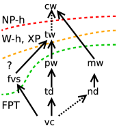
Parameter Result Ref Clique-width paraNP-hard Thm 5.8 Treewidth W[1]-hard Thm 3.20 Pathwidth FPT Thm 4.3 Modular-width FPT Thm 6.12 In the figure, clique-width, treewidth, pathwidth, tree-depth, vertex cover, feedback vertex set, neighborhood diversity, and modular-width are indicated as cw, tw, pw, td, vc, fvs, nd, and mw respectively. Arrows indicate more general parameters. Dotted arrows indicate that the parameter may increase exponentially, (e.g. graphs of vc $k$ have nd at most $2^{k}+k$).

Figure 1: Summary of considered graph parameters and results.

Grundy Coloring

In the Grundy Coloring problem we are given a graph $G=(V,E)$ and are asked to order $V$ in a way that maximizes the number of colors used by the greedy (First-Fit) coloring algorithm. The notion of Grundy coloring was first introduced by Grundy in the 1930s, and later formalized in [19]. Since then, the complexity of Grundy Coloring has been very well-studied (see [1, 3, 16, 33, 48, 50, 57, 61, 82, 84, 86, 87, 88] and the references therein). For the natural parameter, namely the number of colors to be used, Grundy coloring was recently proved to be W[1]-hard in [1]. An XP algorithm for Grundy Coloring parameterized by treewidth was given in [84], using the fact that the Grundy number of any graph is at most $\log n$ times its treewidth. In [15] Bonnet et al. explicitly asked whether this can be improved to an FPT algorithm. They also observed that the problem is FPT parameterized by vertex cover. It appears that the complexity of Grundy Coloring parameterized by pathwidth was never explicitly posed as a question and it was not suspected that it may differ from that for treewidth. We note that, since the problem can be seen to be MSO₁-expressible for a fixed Grundy number (indeed in Definition 2.1 we reformulate it as a coloring problem where each color class dominates later classes, which is an MSO₁-expressible property), it is FPT for all considered parameters if the Grundy number is also a parameter [21], so we intuitively want to concentrate on cases where the Grundy number is large.

Our results

Our results illuminate the complexity of Grundy Coloring parameterized by pathwidth and treewidth, as well as clique-width and modular-width. More specifically:

1. We show that Grundy Coloring is W[1]-hard parameterized by treewidth via a reduction from $k$-Multi-Colored Clique. The main building block of our reduction is the structure of binomial trees, which have treewidth one but unbounded pathwidth, which explains the complexity jump between the two parameters. As mentioned, an XP algorithm is known in this case [84], so this result is in a sense tight.

2. We observe that Grundy Coloring is FPT parameterized by pathwidth. Our main tool here is a combinatorial lemma stating that on any graph the Grundy number is at most a linear function of the pathwidth, which was first shown in [27], using previous results on the First-Fit coloring of interval graphs [58, 74]. To obtain an FPT algorithm we simply combine this lemma with the algorithm of [84].

3. We show that Grundy Coloring is paraNP-complete parameterized by clique-width, that is, NP-complete for graphs of constant clique-width (specifically, clique-width $8$).

4. We show that Grundy Coloring is FPT parameterized by neighborhood diversity (which is defined in [62]) and leverage this result to obtain an FPT algorithm parameterized by modular-width (which is defined in [42]).

Our main interest is concentrated in the first two results, which achieve our goal of finding a natural problem distinguishing pathwidth from treewidth. The result for clique-width nicely fills out the picture by giving an intuitive view of the evolution of the complexity of the problem and showing that in a case where no non-trivial bound can be shown on the optimal value, the problem becomes hopelessly hard from the parameterized point of view.

Other related work

Let us now give a brief survey of “price of generality” results involving our considered parameters, that is, results showing that a problem is efficient for one parameter but hard for a more general one. In this area, the results of Fomin et al. [38], introducing the term “price of generality”, have been particularly impactful. This work and its follow-ups [39, 40], were the first to show that four natural graph problems (Coloring, Edge Dominating Set, Max Cut, Hamiltonicity) which are FPT for treewidth, become W[1]-hard for clique-width. In this sense, these problems, as well as problems discovered later such as counting perfect matchings [22], SAT [77, 25], $\exists\forall$-SAT [66], Orientable Deletion [49], and $d$-Regular Induced Subgraph [18], form part of the “price” we have to pay for considering a more general parameter. This line of research has thus helped to illuminate the complexity border between the two most important sparse and dense parameters (treewidth and clique-width), by giving a list of natural problems distinguishing the two. (An artificial MSO₂-expressible such problem was already known much earlier [21, 64]).

Let us now focus in the area below treewidth in Figure 1 by considering problems which are in XP but W[1]-hard parameterized by treewidth. By now, there is a small number of problems in this category which are known to be W[1]-hard even for vertex cover: List Coloring [34] was the first such problem, followed by CSP (for the vertex cover of the dual graph) [79], and more recently by $(k,r)$-Center, $d$-Scattered Set, and Min Power Steiner Tree [54, 53, 55] on weighted graphs. Intuitively, it is not surprising that problems W[1]-hard parameterized by vertex cover are few and far between, since this is a very restricted parameter. Indeed, for most problems in the literature which are W[1]-hard by treewidth, vertex cover is the only parameter (among the ones considered here) for which the problem becomes FPT.

A second interesting category are problems which are FPT for tree-depth ([75]) but W[1]-hard for pathwidth. Mixed Chinese Postman Problem was the first discovered problem of this type [47], followed by Min Bounded-Length Cut [28, 11], ILP [44], Geodetic Set [56] and unweighted $(k,r)$-Center and $d$-Scattered Set [54, 53]. More recently, $(A,\ell)$-Path Packing was also shown to belong in this category [6].

To the best of our knowledge, for all remaining problems which are known to be W[1]-hard by treewidth, the reductions that exist in the literature also establish W[1]-hardness for pathwidth. Below we give a (semi-exhaustive) list of problems which are known to be W[1]-hard by treewidth. After reviewing the relevant works we have verified that all of the following problems are in fact shown to be W[1]-hard parameterized by pathwidth (and in many case by feedback vertex set and tree-depth), even if this is not explicitly claimed.

1.1 Known problems which are W-hard for treewidth and for pathwidth

• Precoloring Extension and Equitable Coloring are shown to be W[1]-hard for both tree-depth and feedback vertex set in [34] (though the result is claimed only for treewidth). This is important, because Equitable Coloring often serves as a starting point for reductions to other problems. A second hardness proof for this problem was recently given in [24]. These two problems are FPT by vertex cover [36].

• Capacitated Dominating Set and Capacitated Vertex Cover are W[1]-hard for both tree-depth and feedback vertex set [26] (though again the result is claimed for treewidth).

• Min Maximum Out-degree on weighted graphs is W[1]-hard by tree-depth and feedback vertex set [81].

• General Factors is W[1]-hard by tree-depth and feedback vertex set [80].

• Target Set Selection is W[1]-hard by tree-depth and feedback vertex set [10] but FPT for vertex cover [76].

• Bounded Degree Deletion is W[1]-hard by tree-depth and feedback vertex set, but FPT for vertex cover [12, 43].

• Fair Vertex Cover is W[1]-hard by tree-depth and feedback vertex set [60].

• Fixing Corrupted Colorings is W[1]-hard by tree-depth and feedback vertex set [13] (reduction from Precoloring Extension).

• Max Node Disjoint Paths is W[1]-hard by tree-depth and feedback vertex set [32, 37].

• Defective Coloring is W[1]-hard by tree-depth and feedback vertex set [9].

• Power Vertex Cover is W[1]-hard by tree-depth but open for feedback vertex set [2].

• Majority CSP is W[1]-hard parameterized by the tree-depth of the incidence graph [25].

• List Hamiltonian Path is W[1]-hard for pathwidth [71].

• L(1,1)-Coloring is W[1]-hard for pathwidth, FPT for vertex cover [36].

• Counting Linear Extensions of a poset is W[1]-hard (under Turing reductions) for pathwidth [29].

• Equitable Connected Partition is W[1]-hard by pathwidth and feedback vertex set, FPT by vertex cover [31].

• Safe Set is W[1]-hard parameterized by pathwidth, FPT by vertex cover [8].

• Matching with Lower Quotas is W[1]-hard parameterized by pathwidth [4].

• Subgraph Isomorphism is W[1]-hard parameterized by the pathwidth of $G$, even when $G,H$ are connected planar graphs of maximum degree $3$ and $H$ is a tree [70].

• Metric Dimension is W[1]-hard by pathwidth [17]. This was recently strengthened to paraNP-hardness [68], again for pathwidth.

• Simple Comprehensive Activity Selection is W[1]-hard by pathwidth [30].

• Defensive Stackelberg Game for IGL is W[1]-hard by pathwidth (reduction from Equitable Coloring) [5].

• Directed $(p,q)$-Edge Dominating Set is W[1]-hard parameterized by pathwidth [7].

• Maximum Path Coloring is W[1]-hard for pathwidth [63].

• Unweighted $k$-Sparsest Cut is W[1]-hard parameterized by the three combined parameters tree-depth, feedback vertex set, and $k$ [51].

• Graph Modularity is W[1]-hard parameterized by pathwidth plus feedback vertex set [72].

• Minimum Stable Cut is W[1]-hard parameterized by pathwidth [65].

Let us also mention in passing that the algorithmic differences of pathwidth and treewidth may also be studied in the context of problems which are hard for constant treewidth. Such problems also generally remain hard for constant pathwidth (examples are Steiner Forest [46], Bandwidth [73], Minimum mcut [45]). One could also potentially try to distinguish between pathwidth and treewidth by considering the parameter dependence of a problem that is FPT for both. Indeed, for a long time the best-known algorithm for Dominating Set had complexity $3^{k}$ for pathwidth, but $4^{k}$ for treewidth. Nevertheless, the advent of fast subset convolution techniques [85], together with tight SETH-based lower bounds [69] has, for most problems, shown that the complexities on the two parameters coincide exactly.

Finally, let us mention a case where pathwidth and treewidth have been shown to be quite different in a sense similar to our framework. In [78] Razgon showed that a CNF can be compiled into an OBDD (Ordered Binary Decision Diagram) of size FPT in the pathwidth of its incidence graphs, but there exist formulas that always need OBDDs of size XP in the treewidth. Although this result does separate the two parameters, it is somewhat adjacent to what we are looking for, as it does not speak about the complexity of a decision problem, but rather shows that an OBDD-producing algorithm parameterized by treewidth would need XP time simply because it would have to produce a huge output in some cases.

2 Definitions and Preliminaries

For non-negative integers $i,j$, we use $[i,j]$ to denote the set $\{k\ |\ i\leq k\leq j\}$. Note that if $j<i$, then the set $[i,j]$ is empty. We will also write simply $[i]$ to denote the set $[1,i]$.

We give two equivalent definitions of our main problem.

Definition 2.1.

A $k$-Grundy Coloring of a graph $G=(V,E)$ is a partition of $V$ into $k$ non-empty sets $V_{1},\ldots,V_{k}$ such that: (i) for each $i\in[k]$ the set $V_{i}$ induces an independent set; (ii) for each $i\in[k-1]$ the set $V_{i}$ dominates the set $\bigcup_{i<j\leq k}V_{j}$.

Definition 2.2.

A $k$-Grundy Coloring of a graph $G=(V,E)$ is a proper $k$-coloring $c:V\to[k]$ that results by applying the First-Fit algorithm on an ordering of $V$; the First-Fit algorithm colors one by one the vertices in the given ordering, assigning to a vertex the minimum color that is not already assigned to one of its preceding neighbors.

The Grundy number of a graph $G$, denoted by $\Gamma(G)$, is the maximum $k$ such that $G$ admits a $k$-Grundy Coloring. In a given Grundy Coloring, if $u\in V_{i}$ (equiv. if $c(u)=i$) we will say that $u$ was given color $i$. The Grundy Coloring problem is the problem of determining the maximum $k$ for which a graph $G$ admits a $k$-Grundy Coloring. It is not hard to see that a proper coloring is a Grundy coloring if and only if every vertex assigned color $i$ has at least one neighbor assigned color $j$, for each $j<i$.

3 W[1]-Hardness for Treewidth

In this section we prove that Grundy Coloring parameterized by treewidth is W[1]-hard (Theorem 3.20). Our proof relies on a reduction from $k$-Multi-Colored Clique and initially establishes W[1]-hardness for a more general problem where we are given a target color for a set of vertices (Lemma 3.8); we then reduce this to Grundy Coloring.

An interesting aspect of our reduction is that up until a rather advanced point, the instance we construct has not only bounded treewidth (which is necessary for the construction to work), but also bounded pathwidth (see Lemma 3.13). This would seem to indicate that we are headed towards a W[1]-hardness result for Grundy Coloring parameterized by pathwidth, which would contradict the FPT algorithm of Section 4! This is of course not the case, so it is instructive to ponder why the reduction fails to work for pathwidth. The reason this happens is that the final step, which reduces our instance to the plain version of Grundy Coloring needs to rely on a support operation that “pre-colors” some of the vertices and the gadgets we use to achieve this are trees of unbounded Grundy number. The results of Section 4 indicate that if these gadgets have unbounded Grundy number, thay must also have unbounded pathwidth, hence there is a good combinatorial reason why our reduction only works for treewidth.

Let us now present the different parts of our construction. We will make use of the structure of binomial trees $T_{i}$.

Definition 3.1.

The binomial tree $T_{i}$ with root $r_{i}$ is a rooted tree defined recursively in the following way: $T_{1}$ consists simply of its root $r_{1}$; in order to construct $T_{i}$ for $i>1$, we construct one copy of $T_{j}$ for all $j<i$ and a special vertex $r_{i}$, then we connect $r_{j}$ with $r_{i}$. An alternative equivalent definition of the binomial tree $T_{i}$, $i\geq 2$ is that we construct two trees $T_{i-1}$ , $T_{i-1}^{\prime}$, we connect their roots $r_{i-1}$, $r^{\prime}_{i-1}$ and select one of them as the new root $r_{i}$.

Proposition 3.2.

Let $i\geq 2$, $T_{i}$ be a binomial tree and $1\leq t<i$. There exist $2^{i-t-1}$ binomial trees $T_{t}$ which are vertex-disjoint and non-adjacent subtrees in $T_{i}$, where no $T_{t}$ contains the root $r_{i}$ of $T_{i}$.

Proof 3.3.

By induction in $i-t$. For $i-t=1$, $T_{i}$ indeed contains one $T_{i-1}$ that does not contain the root $r_{i}$. Let it be true that $T_{i-1}$ contains $2^{i-t-2}$ subtrees $T_{t}$. Then $T_{i}$ contains two trees $T_{i-1}$ each of which contains $2^{i-t-2}$ $T_{j}$, thus $2^{i-t-1}$ in total.

Proposition 3.4.

$\Gamma(T_{i})\leq i$. Furthermore, for all $j\leq i$ there exists a Grundy coloring which assigns color $j$ to the root of $T_{i}$.

Proof 3.5.

The first part is trivial since in any graph $G$ with maximum degree $\Delta$ we have $\Gamma(G)\leq\Delta+1$. In this case $\Gamma(T_{i})\leq(i-1)+1=i$. For the second part, we first prove that there is a Grundy coloring which assigns color $i$ to the root. This can be proven by strong induction: if for all $k<i$, there is a Grundy coloring which assigns color $k$ to $r_{k}$ for all $1\leq k\leq i-1$, then under this coloring, $r_{i}$ has at least one neighbor receiving color $k$ for all $1\leq k\leq i-1$, so it has to receive color $i$. To assign to the root a color $j<i$ we observe that if $j=1$ this is trivial; if $j>1$, we use the fact that (by inductive hypothesis) there is a coloring that assigns color $j-1$ to $r_{j}$, so in this coloring the root $r_{i}$ will take color $j$.

A Grundy coloring of $T_{i}$ that assigns color $i$ to $r_{i}$ is called optimal. If $r_{i}$ is assigned color $j<i$ then we call the Grundy coloring sub-optimal.

We now define a generalization of the Grundy coloring problem with target colors and show that it is W[1]-hard parameterized by treewidth. We later describe how to reduce this problem to Grundy Coloring such that the treewidth does not increase by a lot.

Definition 3.6 (Grundy Coloring with Targets).

We are given a graph $G(V,E)$, an integer $t\in$ IN called the target and a subset $S\subset V$. (For simplicity we will say that vertices of $S$ have target $t$.) If $G$ admits a Grundy Coloring which assigns color $t$ to some vertex $s\in S$ we say that, for this coloring, vertex $s$ achieves its target. If there exists a Grundy Coloring of $G$ which assigns to all vertices of $S$ color $t$, then we say that $G$ admits a Target-achieving Grundy Coloring. Grundy Coloring with Targets is the decision problem associated to the question “given $G,S,t$ as defined above, does $G$ admit a Target-achieving Grundy Coloring ?”.

We will also make use of the following operation:

Definition 3.7 (Tree-support).

Given a graph $G=(V,E)$, a vertex $u\in V$ and a set $N$ of positive integers, we define the tree-support operation as follows: (a) for all $i\in N$ we add a copy of $T_{i}$ in the graph; (b) we connect $u$ to the root $r_{i}$ of each of the $T_{i}$. We say that we add supports $N$ on $u$. The trees $T_{i}$ will be called the supporting trees or supports of $u$. Slightly abusing notation, we also call supports the numbers $i\in N$.

Intuitively, the tree-support operation ensures that vertex $u$ may have at least one neighbor of color $i$ for each $i\in N$ in a Grundy coloring, and thus increase the color $u$ can take. Observe that adding supporting trees to a vertex does not increase the treewidth, but does increase the pathwidth (binomial trees have unbounded pathwidth).

Our reduction is from $k$-Multi-Colored Clique, proven to be W[1]-hard in [35]: given a $k$-multipartite graph $G=(V_{1},V_{2},\ldots,V_{k},E)$, decide if for every $i\in[k]$ we can pick $u_{i}\in V_{i}$ forming a clique, where $k$ is the parameter. We can also assume that $\forall i\in[k],|V_{i}|=n$, that $n$ is a power of 2, and that $V_{i}=\{v_{i,0},v_{i,1},\ldots,v_{i,n-1}\}$. Furthermore, let $|E|=m$. We construct an instance of Grundy Coloring with Targets $G^{\prime}=(V^{\prime},E^{\prime})$ and $t=2\log n+4$ (where all logarithms are base two) using the following gadgets:

Vertex selection $S_{i,j}$.

See Figure 2(a). This gadget consists of $2\log n$ vertices $S_{i,j}^{1}\cup S_{i,j}^{2}=\bigcup_{l\in[\log n]}\{s_{i,j}^{2l-1}\}\cup\bigcup_{l\in[\log n]}\{s_{i,j}^{2l}\}$, where for each $l\in[\log n]$ we connect vertex $s_{i,j}^{2l-1}$ to $s_{i,j}^{2l}$ thus forming a matching. Furthermore, for each $l\in[2,\log n]$, we add supports $[2l-2]$ to vertices $s_{i,j}^{2l-1}$ and $s_{i,j}^{2l}$. Observe that the vertices $s_{i,j}^{2l-1}$ and $s_{i,j}^{2l}$ together with their supports form a binomial tree $T_{2l}$ with either of these vertices as the root. We construct $k(m+2)$ gadgets $S_{i,j}$, one for each $i\in[k],j\in[0,m+1]$.

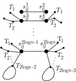
(a) Vertex Selection gadget $S_{i,j}$.

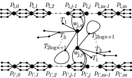
(b) Propagators $p_{i,j}$ and Edge Selection gadget $W_{j}$. The edge selection checkers and the supports of the $p_{i,j}$ and $s_{i,j}^{l}$ are not depicted. In the example $B_{x}=010$ and $B_{y}=100$.

Figure 2: The gadgets. Figure 2(a) is an enlargement of Figure 2(b) between $p_{i,j-1}$ and $p_{i,j}$.

The vertex selection gadget $S_{i,1}$ encodes in binary the vertex that is selected in the clique from $V_{i}$. In particular, for each pair $s_{i,1}^{2l-1},s_{i,1}^{2l}$, $l\in[\log n]$ either of these vertices can take the maximum color in an optimal Grundy coloring of the binomial tree $T_{2l}$ (that is, a coloring that gives the root of the binomial tree $T_{2l}$ color $2l$). A selection corresponds to bit 0 or 1 for the $l^{th}$ binary position. In order to ensure that for each $j\in[m]$ all (middle) $S_{i,j}$ encode the same vertex, we use propagators.

Propagators $p_{i,j}$.

See Figure 2(b). For $i\in[k]$ and $j\in[0,m]$, a propagator $p_{i,j}$ is a single vertex connected to all vertices of $S_{i,j}^{2}\cup S_{i,j+1}^{1}$. To each $p_{i,j}$, we also add supports $\{2\log n+1,2\log n+2,2\log n+3\}$. The propagators have target $t=2\log n+4$.

Edge selection $W_{j}$.

See Figure 2(b). Let $j=(v_{i,x},v_{i^{\prime},y})\in E$, where $v_{i,x}\in V_{i}$ and $v_{i^{\prime},y}\in V_{i^{\prime}}$. The gadget $W_{j}$ consists of four vertices $w_{j,x},w_{j,y},w^{\prime}_{j,x},w^{\prime}_{j,y}$. We call $w^{\prime}_{j,x},w^{\prime}_{j,y}$ the edge selection checkers. We have the edges $(w_{j,x}$, $w_{j,y}),(w^{\prime}_{j,x},w_{j,x}),(w^{\prime}_{j,y},w_{j,y})$. Let us now describe the connections of these vertices with the rest of the graph. Let $B_{x}=b_{1}b_{2}\ldots b_{\log n}$ be the binary representation of $x$. We connect $w_{j,x}$ to each vertex $s_{ij}^{2l-b_{l}}$, $l\in[\log n]$ (we do similarly for $w_{j,y},S_{i^{\prime},j}$, and $B_{y}$). We add to each of $w_{j,x},w_{j,y}$ supports $\bigcup_{l\in[\log n+1]}\{2l-1\}$. We add to each of $w^{\prime}_{j,x},w^{\prime}_{j,y}$ supports $[2\log n+3]\setminus\{2\log n+1\}$ and set the target $t=2\log n+4$ for these two vertices. We construct $m$ such gadgets, one for each edge. We say that $W_{j}$ is activated if at least one of $w_{j,x},w_{j,y}$ receives color $2\log n+3$.

Edge validators $q_{i,i^{\prime}}$.

We construct $k\choose 2$ of these gadgets, one for each pair $(i,i^{\prime}),i<i^{\prime}\in[k]$. The edge validator is a single vertex that is connected to all vertices $w_{j,x}$ for which $j$ is an edge between $V_{i}$ and $V_{i^{\prime}}$. We add supports $[2\log n+2]$ and a target of $t=2\log n+4$.

The edge validator plays the role of an “or” gadget: in order for it to achieve its target, at least one of its neighboring edge selection gadgets should be activated.

Lemma 3.8.

$G$ has a clique of size $k$ if and only if $G^{\prime}$ has a target-achieving Grundy coloring.

Proof 3.9.

$\Rightarrow$) Suppose that $G$ has a clique and we want to produce a coloring of $G^{\prime}$. In the remainder, when we say that we color a support tree “optimally”, we mean that we color its internal vertices in a way that gives the root the maximum possible color.

We color the vertices of $G^{\prime}$ in the following order: First, we color the vertex selection gadget $S_{i,j}$. We start from the supports which we color optimally. We then color the matchings as follows: let $v_{i,x}$ be the vertex that was selected in the clique from $V_{i}$ and $b_{1}b_{2}\ldots b_{\log n}$ be the binary representation of $x$; we color vertices $s_{i,j}^{2l-(1-b_{l})}$, $l\in[\log n]$ with color $2l-1$ and vertices $s_{i,j}^{2l-b_{l}}$, $l\in[\log n]$ will receive color $2l$. For the propagators, we color their supports optimally. Propagators have $2\log n+3$ neighbors each, all with different colors, so they receive color $2\log n+4$, thus achieving the targets.

Then, we color the edge validators $q_{i,i^{\prime}}$ and the edge selection gadgets $W_{j}$ that correspond to edges of the clique (that is, $j=(v_{i,x},v_{i^{\prime},y})\in E$ and $v_{i,x}\in V_{i}$, $v_{i^{\prime},y}\in V_{i^{\prime}}$ are selected in the clique). We first color the supports of $q_{i,i^{\prime}},w_{j,x},w_{j,y}$ optimally. From the construction, vertex $w_{j,x}$ is connected with vertices $s_{i,j}^{2l-b_{l}}$ which have already been colored $2l$, $l\in[\log n]$ and with supports $\bigcup_{l\in[\log n+1]}\{2l-1\}$, thus $w_{j,x}$ will receive color $2\log n+2$. Similarly $w_{j,y}$ already has neighbors which are colored $[2\log n+1]$, but also $w_{j,x}$, thus it will receive color $2\log n+3$. These $W_{j}$ will be activated. Since both $w_{j,x},w_{j,y}$ connect to $q_{i,i^{\prime}}$, the latter will be assigned color $2\log n+4$, thus achieving its target. As for $w^{\prime}_{j,x}$ and $w^{\prime}_{j,y}$, these vertices have one neighbor colored $c$, where $c=2\log n+2$ or $c=2\log n+3$. We color their support $T_{c}$ sub-optimally so that the root receives color $2\log n+1$; we color their remaining supports optimally. This way, vertices $w^{\prime}_{j,x},w^{\prime}_{j,y}$ can be assigned color $t=2\log n+4$, achieving the target.

Finally, for the remaining $W_{j}$, we claim that we can assign to both $w_{j,x},w_{j,y}$ a color that is at least as high as $2\log n+1$. Indeed, we assign to each supporting tree $T_{r}$ of $w_{j,x}$ a coloring that gives its root the maximum color that is $\leq r$ and does not appear in any neighbor of $w_{j,x}$ in the vertex selection gadget. We claim that in this case $w_{j,x}$ will have neighbors with all colors in $[2\log n]$, because in every interval $[2l-1,2l]$ for $l\in[\log n]$, $w_{j,x}$ has a neighbor with a color in that interval and a support tree $T_{2l+1}$. If $w_{j,x}$ has color $2\log n+1$ then we color the supports of $w^{\prime}_{j,x}$ optimally and achieve its target, while if $w_{j,x}$ has color higher than $2\log n+1$, we achieve the target of $w^{\prime}_{j,x}$ as in the previous paragraph.

$\Leftarrow$) Suppose that $G^{\prime}$ admits a coloring that achieves the target for all propagators, edge selection checkers, and edge validators. We will prove the following three claims, which together imply the remaining direction of the lemma:

Claim 1.

The coloring of the vertex selection gadgets is consistent throughout, that is, for each $i\in[k]$ and for each $j_{1},j_{2},l$, we have that $s_{i,j_{1}}^{l},s_{i,j_{2}}^{l}$ received the same color. This coloring corresponds to a selection of $k$ vertices of $G$.

Claim 2.

$k\choose 2$ edge selection gadgets have been activated. They correspond to $k\choose 2$ edges of $G$ being selected.

Claim 3.

If an edge selection gadget $W_{j}=\{w_{j,x},w_{j,y}\}$ with $j=(v_{i,x},v_{i^{\prime},y})$ has been activated then the coloring of the vertex selection gadgets $S_{i,j}$ and $S_{i^{\prime},j}$ corresponds to the selection of vertices $v_{i,x}$ and $v_{i^{\prime},y}$. In other words, selected vertices and edges form a clique of size $k$ in $G$.

Proof 3.10 (Proof of Claim 1).

Suppose that an edge selection checker $w^{\prime}_{j,x}$ achieved its target. We claim that this implies that $w_{j,x}$ has color at least $2\log n+1$. Indeed, $w^{\prime}_{j,x}$ has degree $2\log n+3$, so its neighbors must have all distinct colors in $[2\log n+3]$, but among the supports there are only $2$ neighbors which may have colors in $[2\log n+1,2\log n+3]$. Therefore, the missing color must come from $w_{j,x}$. We now observe that vertices from the vertex selection gadgets have color at most $2\log n$, because if we exclude from their neighbors the vertices $w_{j,x}$ (which we argued have color at least $2\log n+1$) and the propagators (which have target $2\log n+4$), these vertices have degree at most $2\log n-1$.

Suppose that a propagator $p_{i,j}$ achieves its target of $2\log n+4$. Since this vertex has a degree of $2\log n+3$, that means that all of its neighbors should receive all the colors in $[2\log n+3]$. As argued, colors $[2\log n+1,2\log n+3]$ must come from the supports. Therefore, the colors $[2\log n]$ come from the neighbors of $p_{i,j}$ in the vertex selection gadgets.

We now note that, because of the degrees of vertices in vertex selection gadgets, only vertices $s_{i,j}^{2\log n},s_{i,j+1}^{2\log n-1}$ can receive colors $2\log n,2\log n-1$; from the rest, only $s_{i,j}^{2\log n-2},s_{i,j+1}^{2\log n-3}$ can receive colors $2\log n-2,2\log n-3$ etc. Thus, for each $l\in[\log n]$, if $s_{i,j}^{2l}$ receives color $2l-1$ then $s_{i,j+1}^{2l-1}$ should receive color $2l$ and vice versa. With similar reasoning, in all vertex selection gadgets we have that $s_{i,j}^{2l-1},s_{i,j}^{2l}$ received the two colors $\{2l-1,2l\}$ since they are neighbors. As a result, the colors of $s_{i,j+1}^{2l-1}$, $s_{i,j}^{2l-1}$ (and thus the colors of $s_{i,j+1}^{2l}$, $s_{i,j}^{2l}$) are the same, therefore, the coloring is consistent, for all values of $j\in[m]$.

Proof 3.11 (Proof of Claim 2).

If an edge validator achieves its target of $2\log n+4$, then at least one of its neighbors from an edge selection gadget has received color $2\log n+3$. We know that each edge selection gadget only connects to a unique edge validator, so there should be $k\choose 2$ edge selection gadgets which have been activated in order for all edge validators to achieve the target.

Proof 3.12 (Proof of Claim 3).

Suppose that an edge validator $q_{i,i^{\prime}}$ achieves its target. That means that there exists an edge selection gadget $W_{j}=\{w_{j,x},w_{j,y},w^{\prime}_{j,x},w^{\prime}_{j,y}\}$ for which at least one of its vertices $\{w_{j,x},w_{j,y}\}$, say vertex $w_{j,x}$, has received color $2\log n+3$. Let $j$ be an edge connecting $v_{i,x}\in V_{i}$ to $v_{i^{\prime},y}\in V_{i^{\prime}}$. Since the degree of $w_{j,x}$ is $2\log n+4$ and we have already assumed that two of its neighbors ($q_{i,i^{\prime}}$ and $w^{\prime}_{j,x}$) have color $2\log n+4$, in order for it to receive color $2\log n+3$ all its other neighbors should receive all colors in $[2\log n+2]$. The only possible assignment is to give colors $2l$, $l\in[\log n]$ to its neighbors from $S_{i,j}$ and color $2\log n+2$ to $w_{j,y}$. The latter is, in turn, only possible if the neighbors of $w_{j,y}$ from $S_{i^{\prime},j}$ receive all colors $2l$, $l\in[\log n]$. The above corresponds to selecting vertex $v_{i,x}$ from $V_{i}$ and $v_{i^{\prime},y}$ from $V_{i^{\prime}}$.

Lemma 3.13.

Let $G^{\prime\prime}$ be the graph that results from $G^{\prime}$ if we remove all the tree-supports. Then $G^{\prime\prime}$ has pathwidth at most ${k\choose 2}+2k+3$.

Proof 3.14.

We will use the equivalent definition of pathwidth as a node-searching game, where the robber is eager and invisible and the cops are placed on nodes [14]. We will use ${k\choose 2}+2k+4$ cops to clean $G^{\prime\prime}$ as follows: We place $k\choose 2$ cops on the edge validators. Then, starting from $j=0$, we place $2k$ cops on the propagators $p_{i,0},p_{i,1}$ for $i=1,\ldots,k$, plus 2 cops on the edge selection vertices $w_{j,x}$, $w_{j,y}$ that correspond to edge $j$. We use the two additional cops to clean line by line the gadgets $S_{i,j}$. We then use one of these cops to clear $w^{\prime}_{j,x},w^{\prime}_{j,y}$. We continue then to the next column $j=2$ by removing the $k$ cops from the propagators $p_{i,1}$ and placing them to $p_{i,3}$. We continue for $j=3,\ldots m-1$ until the whole graph has been cleaned.

We will now show how to implement the targets using the tree-filling operation defined below.

Definition 3.15 (Tree-filling).

Let $G=(V,E)$ be a graph. Suppose that $S=\{s_{1},s_{2},\ldots,s_{j}\}\subset V$ is a set of vertices with target $t$. The tree-filling operation is the following. First, we add in $G$ a binomial tree $T_{i}$, where $i=\lceil\log j\rceil+t+1$. Observe that, by Proposition 3.2, there exist $2^{i-t-1}>j$ vertex-disjoint and non-adjacent sub-trees $T_{t}$ in $T_{i}$. For each $s\in S$, we find such a copy of $T_{t}$ in $T_{i}$, identify $s$ with its root $r_{t}$, and delete all other vertices of the sub-tree $T_{t}$.

The tree-filling operation might in general increase treewidth, but we will do it in a way such that treewidth only increases by a constant factor compared to the pathwidth of $G$.

Lemma 3.16.

Let $G=(V,E)$ be a graph of pathwidth $w$ and $S=\{s_{1},\ldots,s_{j}\}\subset V$ a subset of vertices having target $t$. Then there is a way to apply the tree-filling operation such that the resulting graph $H$ has $tw(H)\leq 4w+5$.

Proof 3.17.

Construction of $H$. Let $(\mathcal{P},\mathcal{B})$ be a path-decomposition of $G$ whose largest bag has size $w+1$ and $B_{1},B_{2},\ldots,B_{j}\in\mathcal{B}$ distinct bags where $\forall a,s_{a}\in B_{a}$ (assigning a distinct bag to each $s_{a}$ is always possible, as we can duplicate bags if necessary). We call those bags important. We define an ordering $o:S\rightarrow$ I​N of the vertices of $S$ that follows the order of the important bags from left to right, that is $o(s_{a})<o(s_{b})$ if $B_{a}$ is on the left of $B_{b}$ in $\mathcal{P}$. For simplicity, let us assume that $o(s_{a})=a$ and that $B_{a}$ is to the left of $B_{b}$ if $a<b$.

We describe a recursive way to do the substitution of the trees in the tree-filling operation. Crucially, when $j>2$ we will have to select an appropriate mapping between the vertices of $S$ and the disjoint subtrees $T_{t}$ in the added binomial tree $T_{i}$, so that we will be able to keep the treewidth of the new graph bounded.

• If $j=1$ then $i=t+1$. We add to the graph a copy of $T_{i}$, arbitrarily select the root of a copy of $T_{t}$ contained in $T_{i}$, and perform the tree-filling operation as described.

• Suppose that we know how to perform the substitution for sets of size at most $\lceil j/2\rceil$, we will describe the substitution process for a set of size $j$. We have $i=\lceil\log j\rceil+t+1$ and for all $j$ we have $\lceil\log\lceil j/2\rceil\rceil=\lceil\log j\rceil-1$. Split the set $S$ into two (almost) equal disjoint sets $S^{L}$ and $S^{R}$ of size at most $\lceil j/2\rceil$, where for all $s_{a}\in S^{L}$ and for all $s_{b}\in S^{R}$, $a<b$. We perform the tree-filling on each of these sets by constructing two binomial trees $T_{i-1}^{L},T_{i-1}^{R}$ and doing the substitution; then, we connect their roots and set the root of the left tree as the root $r_{i}$ of $T_{i}$, thus creating the substitution of a tree $T_{i}$.

Small treewidth. We now prove that the new graph $H$ that results from applying the tree-filling operation on $G$ and $S$ as described above has a tree decomposition $(\mathcal{T},\mathcal{B^{\prime}})$ of width $4w+5$; in fact we prove by induction on $j$ a stronger statement: if $A,Z\in\mathcal{B}$ are the left-most and right-most bags of $\mathcal{P}$, then there exists a tree decomposition $(\mathcal{T},\mathcal{B^{\prime}})$ of $H$ of width $4w+5$ with the added property that there exists $R\in\mathcal{B^{\prime}}$ such that $A\cup Z\cup\{r_{i}\}\subset R$, where $r_{i}$ is the root of the tree $T_{i}$.

For the base case, if $j=1$ we have added to our graph a $T_{i}$ of which we have selected an arbitrary sub-tree $T_{t}$, and identified the root $r_{t}$ of $T_{t}$ with the unique vertex of $S$ that has a target. Take the path decomposition $(\mathcal{P},\mathcal{B})$ of the initial graph and add all vertices of $A$ (its first bag) and the vertex $r_{i}$ (the root of $T_{i}$) to all bags. Take an optimal tree decomposition of $T_{i}$ of width $1$ and add $r_{i}$ to each bag, obtaining a decomposition of width $2$. We add an edge between the bag of $\mathcal{P}$ that contains the unique vertex of $S$, and a bag of the decomposition of $T_{i}$ that contains the selected $r_{t}$. We now have a tree decomposition of the new graph of width $2w+2<4w+5$. Observe that the last bag of $\mathcal{P}$ now contains all of $A,Z$ and $r_{i}$.

For the inductive step, suppose we applied the tree-filling operation for a set $S$ of size $j>1$. Furthermore, suppose we know how to construct a tree decomposition with the desired properties (width $4w+5$, one bag contains the first and last bags of the path decomposition $\mathcal{P}$ and $r_{i}$), if we apply the tree-filling operation on a target set of size at most $j-1$. We show how to obtain a tree decomposition with the desired properties if the target set has size $j$.

By construction, we have split the set $S$ into two sets $S^{L},S^{R}$ and have applied the tree-filling operation to each set separately. Then, we connected the roots of the two added trees to obtain a larger binomial tree. Observe that for $|S|=j>1$ we have $|S^{L}|,|S^{R}|<j$.

Let us first cut $\mathcal{P}$ in two parts, in such a way that the important bags of $S^{L}$ are on the left and the important bags of $S^{R}$ are on the right. We call $A^{L}=A$ and $Z^{L}$ the leftmost and rightmost bags of the left part and $A^{R}$, $Z^{R}=Z$ the leftmost and rightmost bags of the right part. We define as $G^{L}$ (respectively $G^{R}$) the graph that contains all the vertices of the left (respectively right) part. Let $r_{i}$ be the root of $T_{i}$ and $r_{i-1}$ the root of its subtree $T_{i-1}$. From the inductive hypothesis, we can construct tree decompositions $(\mathcal{T^{L},B^{L}})$, $(\mathcal{T^{R},B^{R}})$ of width $4w+5$ for the graphs $H^{L}$, $H^{R}$ that occur after applying tree-filling on $G^{L},S^{L}$ and $G^{R},S^{R}$; furthermore, there exist $R^{L}\in\mathcal{B^{L}},R^{R}\in\mathcal{B^{R}}$ such that $R^{L}\supseteq A\cup Z^{L}\cup\{r_{i}\}$ and $R^{R}\supseteq A^{R}\cup Z\cup\{r_{i-1}\}$.

We construct a new bag $R^{\prime}=A\cup A^{R}\cup Z^{L}\cup Z\cup\{r_{i-1},r_{i}\}$, and we connect $R^{\prime}$ to both $R^{L}$ and $R^{R}$, thus combining the two tree-decompositions into one. Last we create a bag $R=A\cup Z\cup\{r_{i}\}$ and attach it to $R^{\prime}$. This completes the construction of $(\mathcal{T,B^{\prime}})$.

Observe that $(\mathcal{T,B^{\prime}})$ is a valid tree-decomposition for $H$:

• $V(H)=V(H^{L})\cup V(H^{R})$, thus $\forall v\in V(H),v\in\mathcal{B^{L}}\cup\mathcal{B^{R}}\subset\mathcal{B}$.

• $E(H)=E(H^{L})\cup E(H^{R})\cup\{(r_{i-1},r_{i})\}$. We have that $r_{i-1},r_{i}\in R^{\prime}\in\mathcal{B}$. All other edges were dealt with in $\mathcal{T^{L},T^{R}}$.

• Each vertex $v\in V(H)$ that belongs in exactly one of $H^{L},H^{R}$ trivially satisfied the connectivity requirement: bags that contain $v$ are either fully contained in $\mathcal{T^{L}}$ or $\mathcal{T^{R}}$. A vertex $v$ that is in both $H^{L}$ and $H^{R}$ is also in $Z^{L}\cap A^{R}$ due to the properties of path-decompositions, hence in $R^{\prime}$. Therefore, the sub-trees of bags that contain $v$ in $\mathcal{T^{L},T^{R}}$, form a connected sub-tree in $\mathcal{T}$.

The width of $\mathcal{T}$ is $\max\{tw(H^{L}),tw(H^{R}),|R^{\prime}|-1\}=4w+5$.

The last thing that remains to do in order to complete the proof is to show the equivalence between achieving the targets and finding a Grundy coloring.

Lemma 3.18.

Let $G$ and $G^{\prime}$ be two graphs as described in Lemma 3.8 and let $H$ be constructed from $G^{\prime}$ by using the tree-filling operation. Then $G$ has a clique of size $k$ if and only if $\Gamma(H)\geq\lceil\log(k(m+1)+{k\choose 2}+2m)\rceil+2\log n+5$. Furthermore, $tw(H)\leq 4{k\choose 2}+8k+17$.

Proof 3.19.

We note that the number of vertices with targets in our construction is $m^{\prime}=k(m+1)+{k\choose 2}+2m$ (the propagators, edge selection checkers, and edge-checkers). From Lemma 3.8, it only suffices to show that $\Gamma(H)\geq\lceil\log m^{\prime}\rceil+2\log n+5$ if and only if the vertices with targets achieve color $t=2\log n+4$.

For the forward direction, once vertices with targets get the desirable colors, the rest of the binomial tree of the tree-filling operation can be colored optimally, starting from its leaves all the way up to its roots, which will get color $i=\lceil\log m^{\prime}\rceil+2\log n+5$.

For the converse direction, observe that the only vertices having degree higher than $2\log n+4$ are the edge-checkers and the vertices of the binomial tree $H\setminus G^{\prime}$. However, the edge-checkers connect to only one vertex of degree higher than $2\log n+4$, that in the binomial tree. Thus no vertex of $G^{\prime}$ can ever get a color higher than $2\log n+6$ and the only way that $\Gamma(H)\geq\lceil\log m^{\prime}\rceil+2\log n+5$ is if the root of the binomial tree of the tree-filling operation (the only vertex of high enough degree) receives color $\lceil\log m^{\prime}\rceil+2\log n+5$. For that to happen, all the support-trees of this tree should be colored optimally, which proves that the vertices with targets $2\log n+4$ having substituted support trees $T_{2\log n+4}$ should achieve their targets.

In terms of the treewidth of $H$ we have the following: Lemma 3.13 says that $G^{\prime}$ once we remove all the supporting trees has pathwidth at most ${k\choose 2}+2k+3$. Applying Lemma 3.16 we get that $H$ where we have ignored the tree-supports from $G^{\prime}$ has treewidth at most $4\left({k\choose 2}+2k+3\right)+5$. Adding back the tree-supports does not increase its treewidth.

The main theorem of this section now immediately follows.

Theorem 3.20.

Grundy Coloring parameterized by treewidth is W[1]-hard.

4 FPT for pathwidth

In this section, we show that, in contrast to treewidth, Grundy Coloring is FPT parameterized by pathwidth. This is achieved by a combination of an algorithm for Grundy Coloring  given by Telle and Proskurowski and a combinatorial bound due to Dujmovic, Joret, and Wood. We first recall these results below.

Lemma 4.1 ([27]).

For every graph $G$, $\Gamma(G)\leq 8\cdot(pw(G)+1)$.

Lemma 4.2 ([84]).

There is an algorithm which solves Grundy Coloring  in time $O^{*}(2^{O(tw(G)\cdot\Gamma(G))})$.

We thus get the following result.

Theorem 4.3.

Grundy Coloring can be solved in time $O^{*}(2^{O(pw(G)^{2})})$.

Proof 4.4.

Since in all graphs $tw(G)\leq pw(G)$ and by Lemma 4.1 $\Gamma(G)\leq 8(pw(G)+1)$, we have $tw(G)\cdot\Gamma(G)=O(pw(G)^{2})$ and the algorithm of [84] runs in at most the stated time.

5 NP-hardness for Constant Clique-width

In this section we prove that Grundy Coloring is NP-hard even for constant clique-width via a reduction from 3-SAT. We use a similar idea of adding supports as in Section 3, but supports now will be cliques instead of binomial trees. The support operation is defined as:

Definition 5.1.

Given a graph $G=(V,E)$, a vertex $u\in V$ and a set of positive integers $S$, we define the support operation as follows: for each $i\in S$, we add to $G$ a clique of size $i$ (using new vertices) and we connect one arbitrary vertex of each such clique to $u$.

When applying the support operation we will say that we support vertex $u$ with set $S$ and we will call the vertices introduced supporting vertices. Intuitively, the support operation ensures that the vertex $u$ may have at least one neighbor with color $i$ for each $i\in S$.

We are now ready to describe our construction. Suppose we are given a 3CNF formula $\phi$ with $n$ variables $x_{1},\ldots,x_{n}$ and $m$ clauses $c_{1},\ldots,c_{m}$. We assume without loss of generality that each clause contains exactly three variables. We construct a graph $G(\phi)$ as follows:

1. For each $i\in[n]$ we construct two vertices $x_{i}^{P},x_{i}^{N}$ and the edge $(x_{i}^{P},x_{i}^{N})$.

2. For each $i\in[n]$ we support the vertices $x_{i}^{P},x_{i}^{N}$ with the set $[2i-2]$. (Note that $x_{1}^{P},x_{1}^{N}$ have empty support).

3. For each $i\in[n],j\in[m]$, if variable $x_{i}$ appears in clause $c_{j}$ then we construct a vertex $x_{i,j}$. Furthermore, if $x_{i}$ appears positive in $c_{j}$, we connect $x_{i,j}$ to $x_{i^{\prime}}^{P}$ for all $i^{\prime}\in[n]$; otherwise we connect $x_{i,j}$ to $x_{i^{\prime}}^{N}$ for all $i^{\prime}\in[n]$.

4. For each $i\in[n],j\in[m]$ for which we constructed a vertex $x_{i,j}$ in the previous step, we support that vertex with the set $(\{2k\ |\ k\in[n]\}\cup\{2i-1,2n+1,2n+2\})\setminus\{2i\}$.

5. For each $j\in[m]$ we construct a vertex $c_{j}$ and connect to all (three) vertices $x_{i,j}$ already constructed. We support the vertex $c_{j}$ with the set $[2n]$.

6. For each $j\in[m]$ we construct a vertex $d_{j}$ and connect it to $c_{j}$. We support $d_{j}$ with the set $[2n+3]\cup[2n+5,2n+3+j]$.

7. We construct a vertex $u$ and connect it to $d_{j}$ for all $j\in[m]$. We support $u$ with the set $[2n+4]\cup[2n+5+m,10n+10m]$.

This completes the construction. Before we proceed, let us give some intuition. Observe that we have constructed two vertices $x_{i}^{P},x_{i}^{N}$ for each variable. The support of these vertices and the fact that they are adjacent, allow us to give them colors $\{2i-1,2i\}$. The choice of which gets the higher color encodes an assignment to variable $x_{i}$. The vertices $x_{i,j}$ are now supported in such a way that they can “ignore” the values of all variables except $x_{i}$; for $x_{i}$, however, $x_{i,j}$ “prefers” to be connected to a vertex with color $2i$ (since $2i-1$ appears in the support of $x_{i,j}$, but $2i$ does not). Now, the idea is that $c_{j}$ will be able to get color $2n+4$ if and only if one of its literal vertices $x_{i,j}$ was “satisfied” (has a neighbor with color $2i$). The rest of the construction checks if all clause vertices are satisfied in this way.

We now state the lemmata that certify the correctness of our reduction.

Lemma 5.2.

If $\phi$ is satisfiable then $G(\phi)$ has a Grundy coloring with $10n+10m+1$ colors.

Proof 5.3.

Consider a satisfying assignment of $\phi$. We first produce a coloring of the vertices $x_{i}^{P},x_{i}^{N}$ as follows: if $x_{i}$ is set to True, then $x_{i}^{P}$ is colored $2i$ and $x_{i}^{N}$ is colored $2i-1$; otherwise $x_{i}^{P}$ is colored $2i-1$ and $x_{i}^{N}$ is colored $2i$. Before proceeding, let us also color the supporting vertices of $x_{i}^{P},x_{i}^{N}$: each such vertex belongs to a clique which contains only one vertex with a neighbor outside the clique. For each such clique of size $\ell$, we color all vertices of the clique which have no outside neighbors with colors from $[\ell-1]$ and use color $\ell$ for the remaining vertex. Note that the coloring we have produced so far is a valid Grundy coloring, since each vertex $x_{i}^{P},x_{i}^{N}$ has for each $c\in[2i-2]$ a neighbor with color $c$ among its supporting vertices, allowing us to use colors $\{2i-1,2i\}$ for $x_{i}^{P},x_{i}^{N}$. In the remainder, we will use similar such colorings for all supporting cliques. We will only stress the color given to the vertex of the clique that has an outside neighbor, respecting the condition that this color is not larger than the size of the clique. Note that it is not a problem if this color is strictly smaller than the size of the clique, as we are free to give higher colors to internal vertices.

Consider now a clause $c_{j}$ for some $j\in[m]$. Suppose that this clause contains the three variables $x_{i_{1}},x_{i_{2}},x_{i_{3}}$. Because we started with a satisfying assignment, at least one of these variables has a value that satisfies the clause, without loss of generality $x_{i_{3}}$. We therefore color $x_{i_{1}},x_{i_{2}},x_{i_{3}}$ with colors $2n+1,2n+2,2n+3$ respectively and we color $c_{j}$ with color $2n+4$. We now need to show that we can appropriately color the supporting vertices to make this a valid Grundy coloring.

Recall that the vertex $x_{i_{3}}$ has support $\{2,4,\ldots,2n\}\setminus\{2i_{3}\}\cup\{2i_{3}-1,2n+1,2n+2\}$. For each $i^{\prime}\neq i_{3}$ we observe that $x_{i_{3}}$ is connected to a vertex (either $x_{i_{3}}^{P}$ or $x_{i_{3}}^{N}$) which has a color in $\{2i^{\prime}-1,2i^{\prime}\}$, we are therefore missing the other color from this set. We consider the clique of size $2i^{\prime}$ supporting $x_{i_{3},j}$: we assign this missing color to the vertex of this clique that is adjacent to $x_{i_{3},j}$. Note that the clique is large enough to color its remaining vertices with lower colors in order to make this a valid Grundy coloring. For $i_{3}$, we observe that, since $x_{i_{3}}$ satisfies the clause, the vertex $x_{i_{3},j}$ has a neighbor (either $x_{i_{3}}^{P}$ or $x_{i_{3}}^{N}$) which has received color $2i_{3}$; we use color $2i_{3}-1$ in the support clique of the same size. Similarly, we use colors $2n+1,2n+2$ in the support cliques of the same sizes, and $x_{i_{3}}$ has neighbors with colors covering all of $[2n+2]$.

For the vertex $x_{i_{2},j}$ we proceed in a similar way. For $i^{\prime}<i_{2}$ we give the support vertex from the clique of size $2i^{\prime}$ the color from $\{2i^{\prime}-1,2i^{\prime}\}$ which does not already appear in the neighborhood of $x_{i_{2},j}$. For $i^{\prime}\in[i_{2},n-1]$ we take the vertex from the clique of size $2i^{\prime}+2$ and give it the color of $\{2i^{\prime}-1,2i^{\prime}\}$ which does not yet appear in the neighborhood of $x_{i_{2},j}$. In this way we cover all colors in $[2n-2]$. We now observe that $x_{i_{2},j}$ has a neighbor with color in $\{2n-1,2n\}$ (either $x_{n}^{P}$ or $x_{n}^{N}$); together with the support vertices from the cliques of sizes $2n+1,2n+2$ this allows us to cover the colors $[2n-1,2n+1]$. We use a similar procedure to cover the colors $[2n]$ in the neighborhood of $x_{i_{1},j}$. Now, the $2n$ support vertices in the neighborhood of $c_{j}$, together with $x_{i_{1},j},x_{i_{2},j},x_{i_{3},j}$ allow us to give that vertex color $2n+4$.

We now give each vertex $d_{j}$, for $j\in[m]$ color $2n+j+4$. This can be extended to a valid coloring, because $d_{j}$ is adjacent to $c_{j}$, which has color $2n+4$, and the support of $d_{j}$ is $[2n+j+3]\setminus\{2n+4\}$.

Finally, we give $u$ color $10n+10m+1$. Its support is $[10n+10m]\setminus[2n+5,2n+m+4]$. However, $u$ is adjacent to all vertices $d_{j}$, whose colors cover the set $\{2n+4+j\ |\ j\in[m]\}$.

Lemma 5.4.

If $G(\phi)$ has a Grundy coloring with $10n+10m+1$ colors, then $\phi$ is satisfiable.

Proof 5.5.

Consider a Grundy coloring of $G(\phi)$. We first assume without loss of generality that we consider a minimal induced subgraph of $G$ for which the coloring remains valid, that is, deleting any vertex will either reduce the number of colors or invalidate the coloring. In particular, this means there is a unique vertex with color $10n+10m+1$. This vertex must have degree at least $10n+10m$. However, there are only two such vertices in our graph: $u$ and its support neighbor vertex in the clique of size $10n+10m$. If the latter vertex has color $10n+10m+1$, we can infer that $u$ has color $10n+10m$: this color cannot appear in the clique because all its internal vertices have degree $10n+10m-1$, and one of their neighbors has a higher color. We observe now that exchanging the colors of $u$ and its neighbor produces another valid coloring. We therefore assume without loss of generality that $u$ has color $10n+10m+1$.

We now observe that in each supporting clique of $u$ of size $i$ the maximum color used is $i$ (since $u$ has the largest color in the graph). Similarly, the largest color that can be assigned to $d_{j}$ is $2n+j+4$, because $d_{j}$ has degree $2n+j+4$, but one of its neighbors ($u$) has a higher color. We conclude that the only way for the $10n+10m$ neighbors of $u$ to cover all colors in $[10n+10m]$ is for each support clique of size $i$ to use color $i$ and for each $d_{j}$ to be given color $2n+j+4$.

Suppose now that $d_{j}$ was given color $2n+j+4$. This implies that the largest color that $c_{j}$ may have received is $2n+4$, since its degree is $2n+4$, but $d_{j}$ received a higher color. We conclude again that for the neighbors of $d_{j}$ to cover $[2n+j+3]$ it must be the case that each supporting clique used its maximum possible color and $c_{j}$ received color $2n+4$.

Suppose now that a vertex $c_{j}$ received color $2n+4$. Since $d_{j}$ received a higher color, the remaining $2n+3$ neighbors of this vertex must cover $[2n+3]$. In particular, since the support vertices have colors in $[2n]$, its three remaining neighbors, say $x_{i_{1},j},x_{i_{2},j},x_{i_{3},j}$ must have colors covering $[2n+1,2n+3]$. Therefore, all vertices $x_{i,j}$ have colors in $[2n+1,2n+3]$.

Consider now two vertices $x_{i}^{P},x_{i}^{N}$, for some $i\in[n]$. We claim that the vertex which among these two has the lower color, has color at most $2i-1$. To see this observe that this vertex may have at most $2i-2$ neighbors from the support vertices that have lower colors and these must use colors in $[2i-2]$ because of their degrees. Its neighbors of the form $x_{i,j}$ have color at least $2n+1>2i-1$, and its neighbor in $\{x_{i}^{P},x_{i}^{N}\}$ has a higher color. Therefore, the smaller of the two colors used for $\{x_{i}^{P},x_{i}^{N}\}$ is at most $2i-1$ and by similar reasoning the higher of the two colors used for this set is at most $2i$. We now obtain an assignment for $\phi$ by setting $x_{i}$ to True if $x_{i}^{P}$ has a higher color than $x_{i}^{N}$ and False otherwise (this is well-defined, since $x_{i}^{P},x_{i}^{N}$ are adjacent).

Let us argue why this is a satisfying assignment. Take a clause vertex $c_{j}$. As argued, one of its neighbors, say $x_{i_{3},j}$ has color $2n+3$. The degree of $x_{i_{3},j}$, excluding $c_{j}$ which has a higher color, is $2n+2$, meaning that its neighbors must exactly cover $[2n+2]$ with their colors. Since vertices $x_{i}^{P},x_{i}^{N}$ have color at most $2i$, the colors $[2n+1,2n+2]$ must come from the support cliques of the same sizes. Now, for each $i\in[n]$ the vertex $x_{i_{3},j}$ has exactly two neighbors which may have received colors in $\{2i-1,2i\}$. This can be seen by induction on $i$: first, for $i=n$ this is true, since we only have the support clique of size $2n$ and the neighbor in $\{x_{n}^{P},x_{n}^{N}\}$. Proceeding in the same way we conclude the claim for smaller values of $i$. The key observation is now that the clique of size $2i_{3}-1$ cannot give us color $2i_{3}$, therefore this color must come from $\{x_{i_{3}}^{N},x_{i_{3}}^{P}\}$. If the neighbor of $x_{i_{3},j}$ in this set uses $2i_{3}$, this must be the higher color in this set, meaning that $x_{i_{3}}$ has a value that satisfies $c_{j}$.

Lemma 5.6.

The graph $G(\phi)$ has clique-width at most 8.

Proof 5.7 (Lemma 5.6).

Let us first observe that the support operation does not significantly affect a graph’s clique-width. Indeed, if we have a clique-width expression for $G(\phi)$ without the support vertices, we can add these vertices as follows: each time we introduce a vertex that must be supported we instead construct the graph induced by this vertex and its support and then rename all supporting vertices to a junk label that is never connected to anything else. It is clear that this can be done by adding at most three new labels: two labels for constructing the clique (that will form the support gadget) and the junk label. In fact, below we give a clique-width expression for the rest of the graph that already uses a junk label (say, label $0$), that is, a label on which we never apply a Join operation. Hence, it suffices to compute the clique-width of $G(\phi)$ without the support gadgets and then add $2$.

Let us then argue why the rest of the graph has constant clique-width. First, the graph induced by $x_{i}^{N},x_{i}^{P}$, for $i\in[n]$ is a matching. We construct this graph using $4$ labels, say $1,2,3,4$ as follows: for each $i\in[n]$ we introduce $x_{i}^{N}$ with label $3$, $x_{i}^{P}$ with label $4$, perform a Join between labels $3$ and $4$, then Rename label $3$ to $1$ and label $4$ to $2$. This constructs the matching induced by these $2n$ vertices and also ensures that all vertices $x_{i}^{N}$ have label $1$ in the end and all vertices $x_{i}^{P}$ have label $2$ in the end.

We then introduce to the graph the clauses one by one. Specifically, for each $j\in[m]$ we do the following: we introduce $c_{j}$ with label $3$, $d_{j}$ with label $4$, Join labels $3$ and $4$, Rename label $4$ to label $5$; then for each $i\in[n]$ such that we have a vertex $x_{i,j}$ we introduce that vertex with label $4$, Join label $4$ with label $3$, and Join label $4$ with label $1$ or $2$, depending on whether $x_{i,j}$ is connected to vertices $x_{i}^{N}$ or $x_{i}^{P}$, then Rename label $4$ to the junk label $0$. Once all $x_{i,j}$ vertices for a fixed $j$ have been introduced we Rename label $3$ to the junk label $0$ and move to the next clause. Finally, we introduce $u$ with label $3$ and Join label $3$ to label $5$ (which is the label shared by all $d_{j}$ vertices). In the end we have used $6$ labels, namely the labels $\{0,1,2,3,4,5\}$ for $G(\phi)$ without the support vertices, so the whole graph can be constructed with $8$ labels.

Theorem 5.8.

Given graph $G=(V,E)$, $k$-Grundy Coloring is NP-hard even when the clique-width of the graph $cw(G)$ is a fixed constant.

6 FPT for modular-width

In this section we show that Grundy Coloring is FPT parameterized by modular-width. Recall that $G=(V,E)$ has modular-width $w$ if $V$ can be partitioned into at most $w$ modules, such that each module is a singleton or induces a graph of modular-width $w$. Neighborhood diversity is the restricted version of this measure where modules are required to be cliques or independent sets.

The first step is to show that Grundy Coloring is FPT parameterized by neighborhood diversity. Similarly to the standard Coloring algorithm for this parameter [62], we observe that, without loss of generality, all modules can be assumed to be cliques, and hence any color class has one of $2^{w}$ possible types, depending on the modules it intersects. We would like to use this to reduce the problem to an ILP with $2^{w}$ variables, but unlike Coloring, the ordering of color classes matters. We thus prove that the optimal solution can be assumed to have a “canonical” structure where each color type only appears in consecutive colors. We then extend the neighborhood diversity algorithm to modular-width using the idea that we can calculate the Grundy number of each module separately, and then replace it with an appropriately-sized clique.

6.1 Neighborhood diversity

Recall that two vertices $u,v\in V$ of a graph $G=(V,E)$ are twins if $N(u)\setminus\{v\}=N(v)\setminus\{u\}$, and they are called true (respectively, false) twins if they are adjacent (respectively, non-adjacent). A twin class is a maximal set of vertices that are pairwise twins. It is easy to see that any twin class is either a clique or an independent set. We say that a graph $G=(V,E)$ has neighborhood diversity $w$ if $V$ can be partitioned into at most $w$ twin classes.

Let $G=(V,E)$ be a graph of neighborhood diversity $w$ with a vertex partition $V=W_{1}\dot{\cup}\ldots\dot{\cup}W_{w}$ into twin classes. It is obvious that in any Grundy Coloring of $G$, the vertices of a true twin class must have all distinct colors because they form a clique. Furthermore, it is not difficult to see that the vertices of a false twin class must be colored by the same color because all of their vertices have the same neighbors.

In fact, we can show that we can remove vertices from a false twin class without affecting the Grundy number of the graph:

Lemma 6.1.

Let $G=(V,E)$ be a graph of neighborhood diversity $w$ with a vertex partition $V=W_{1}\dot{\cup}\ldots\dot{\cup}W_{w}$ into twin classes. Let $W_{i}$ be a false twin class having at least two distinct vertices $u,v\in W_{i}$. Then $G-v$ has $k$-Grundy coloring if and only if $G$ has.

Proof 6.2.

The forward implication is trivial. To see the opposite direction, consider an arbitrary $k$-Grundy coloring of $G$. The vertices $u,v$ must have the same color, since they have the same neighbors. Any vertex whose color is higher than $v$ and is adjacent with $v$ must be to $u$ as well. Since $u$ and $v$ have the same color, this implies that the same coloring restricted to $G-v$ is a $k$-Grundy coloring.

Using Lemma 6.1, we can reduce every false twin class into a singleton vertex, thus from now on we may assume that every twin class is a clique (possibly a singleton). An immediate consequence is that that any color class of a Grundy coloring can take at most one vertex from each twin class. Furthermore, the colors of any two vertices from the same twin class are interchangeable. Therefore, a color class $V_{i}$ of a Grundy coloring is precisely characterized by the set of twin classes $W_{j}$ that $V_{i}$ intersects. For a color class $V_{i}$, we call the set $\{j\in[w]:W_{j}\cap V_{i}\neq\emptyset\}$ as the intersection pattern of $V_{i}$.

Let $\cal{I}$ be the collection of all sets $I\subseteq[w]$ of indices such that $W_{i}$ and $W_{j}$ are non-adjacent for every distinct pairs $i,j\in[w]$. It is clear that the intersection pattern of any color class is a member of $\cal{I}$. It turns out that if $I\in\cal{I}$ appears as an intersection pattern for more than one color classes, then it can be assumed to appear on a consecutive set of colors.

Lemma 6.3.

Let $G=(V,E)$ be a graph of neighborhood diversity $w$ with a vertex partition $V=W_{1}\dot{\cup}\ldots\dot{\cup}W_{w}$ into true twin classes. Let $V_{1}\dot{\cup}\ldots\dot{\cup}V_{k}$ be a $k$-Grundy coloring of $G$ and let $I_{i}\in\cal{I}$ be the set of indices $j$ such that $V_{i}\cap W_{j}\neq\emptyset$ for each $i\in[k]$. If $I_{i}=I_{i^{\prime}}$ for some $i^{\prime}\geq i+2$, then the coloring $V^{\prime}_{1}\dot{\cup}\ldots\dot{\cup}V^{\prime}_{k}$ where

$$V^{\prime}_{\ell}=\begin{cases}V_{i^{\prime}}&\text{if }\ell=i+1,\\ V_{\ell-1}&\text{if }i+1<\ell\leq i^{\prime},\\ V_{\ell}&\text{otherwise}\end{cases}$$

(i.e. the coloring obtained by ‘inserting’ $V_{i^{\prime}}$ in between $V_{i}$ and $V_{i+1}$) is a Grundy coloring as well.

Proof 6.4.

First observe that the new coloring remains a proper coloring, so we only need to argue that it’s a valid Grundy coloring. Consider a vertex $v$ which took color $j\leq i$ in the original coloring. All its neighbors with color strictly smaller than $j$ have retained their colors, so $v$ is still properly colored. Suppose then that $v$ had color $j>i^{\prime}$ in the original coloring. Then, $v$ has a neighbor in each of the classes $V_{1},\ldots,V_{j-1}$, which means that it has at least one neighbor in each of the sets $V^{\prime}_{1},\ldots,V^{\prime}_{j-1}$, so it is still validly colored.

Suppose that $v$ had received a color $j\in[i+1,i^{\prime}-1]$ in the original coloring and receives color $j+1$ in the new coloring. We claim that for each $j^{\prime}<j+1$, $v$ has a neighbor with color $j^{\prime}$. Indeed, this is easy to see for $j^{\prime}\leq i$, as these vertices retain their colors; for $j^{\prime}=i+1$ we observe that $v$ has a neighbor with color $i$ in the original coloring, and each such vertex has a true twin with color $i+1$ in the new coloring; and for $j^{\prime}>i+1$, the neighbor of $v$ which had color $j^{\prime}-1$ originally now has color $j^{\prime}$.

Finally, suppose that $v$ had received color $i^{\prime}$ in the original coloring and receives color $i+1$ in the new coloring. We now observe that such a vertex $v$ must have a true twin which received color $i$ in both colorings, therefore coloring $v$ with $i+1$ is valid.

The following is a consequence of Lemma 6.3.

Corollary 6.5.

Let $G=(V,E)$ be a graph of neighborhood diversity $w$ with a vertex partition $V=W_{1}\dot{\cup}\ldots\dot{\cup}W_{w}$ into true twin classes. If $G$ admits a $k$-Grundy coloring, then there is a $k$-Grundy coloring $V_{1}\dot{\cup}\ldots\dot{\cup}V_{k}$ with the following property: for each $j_{1},j_{2}\in[k]$ such that $V_{j_{1}}$ has a non-empty intersection with the same twin classes as $V_{j_{2}}$, we have that for all $j_{3}\in[k]$ with $j_{1}\leq j_{3}\leq j_{2}$, $V_{j_{3}}$ also has non-empty intersection with the same twin classes as $V_{j_{1}}$.

For a sub-collection $\cal{I}^{\prime}$ of $\cal{I}$, we say that $\cal{I}^{\prime}$ is eligible if there is an ordering $\preceq$ on $\cal{I}^{\prime}$ such that for every $I,I^{\prime}\in\cal{I}^{\prime}$ with $I\succeq I^{\prime}$, and for every $i\in I$, there exists $i^{\prime}\in I^{\prime}$ such that the twin classes $W_{i}$ and $W_{i^{\prime}}$ are adjacent, or $i=i^{\prime}$. Clearly, a sub-collection of an eligible sub-collection of $\cal{I}$ is again eligible. Intuitively, the ordering that shows that a sub-collection is eligible corresponds to a Grundy coloring where color classes have the corresponding intersection patterns.

Now we are ready to present an FPT algorithm, parameterized by the neighborhood diversity $w$, to compute the Grundy number. The algorithm consists of two steps: (i) guess a sub-collection $\cal{I}^{\prime}$ of $\cal{I}$ which are used as intersection patterns by a Grundy coloring, and (ii) given $\cal{I}^{\prime}$, we solve an integer linear program.

Let $\cal{I}^{\prime}$ be a sub-collection of $\cal{I}$. For each $I\in\cal{I}^{\prime}$, let $x_{I}$ be an integer variable which is interpreted as the number of colors for which $I$ appears as an intersection pattern. Now, the linear integer program ILP($\cal{I}^{\prime}$) for a sub-collection $\cal{I}^{\prime}$ is given as the following:

(1) $$\max\sum_{I\in\cal{I}^{\prime}}x_{I}$$

(2) s.t.

$$\sum_{I\in{\cal I}^{\prime}:i\in I}x_{I}=|W_{i}|\qquad\forall i\in[w],$$

where each $x_{I}$ takes a positive integer value.

Lemma 6.6.

Let $G=(V,E)$ be a graph of neighborhood diversity $w$ with a vertex partition $V=W_{1}\dot{\cup}\ldots\dot{\cup}W_{w}$ into true twin classes. The maximum value of ILP($\cal{I}^{\prime}$) over all eligible $\cal{I}^{\prime}\subseteq\cal{I}$ equals the Grundy number of $G$.

Proof 6.7.

We first prove that the maximum value over all considered ILPs is at least the Grundy number of $G$. Fix a Grundy coloring $V_{1}\dot{\cup}\cdots\dot{\cup}V_{k}$ achieving the Grundy number while satisfying the condition of Corollary 6.5. Consider the sub-collection $\cal{I}^{\prime}$ of $\cal I$ used as intersection patterns in the fixed Grundy coloring. It is clear that $\cal{I}^{\prime}$ is eligible, using the natural ordering of the color classes. Let $\bar{x}_{I}$ be the number of colors for which $I$ is an intersection pattern for each $I\in\cal{I}^{\prime}$. It is straightforward to check that setting the variable $x_{I}$ at value $\bar{x}_{I}$ satisfies the constraints of ILP($\cal{I}^{\prime}$), because all vertices of each twin class are colored exactly once. Therefore, the objective value of ILP($\cal{I}^{\prime}$) is at least the Grundy number.

To establish the opposite direction of inequality, let $\cal{I}^{\prime}$ be an eligible sub-collection of $\cal{I}$ achieving the maximum ILP objective value. Notice that ILP($\cal{I}^{\prime}$) is feasible, and let $x^{*}_{I}$ be the value taken by the variable $x_{I}$ for each $I\in\cal{I}^{\prime}$. Since $\cal{I}^{\prime}$ is eligible, there exists an ordering $\preceq$ on $\cal{I}^{\prime}$ such that for every $I,I^{\prime}\in\cal{I}^{\prime}$ with $I\succeq I^{\prime}$, and for every $i\in I$, there exists $i^{\prime}\in I^{\prime}$ such that the twin classes $W_{i}$ and $W_{i^{\prime}}$ are adjacent. Now, we can define the coloring $V_{1}\dot{\cup}\cdots\dot{\cup}V_{\ell}$ by taking the first (i.e. minimum element in $\preceq$) element $I_{1}$ of $\cal I^{\prime}$ $x^{*}_{I}$ times. That is, each of $V_{1}$ up to $V_{x^{*}_{I_{1}}}$ contains precisely one vertex of $W_{i}$ for each $i\in I$. The succeeding element $I_{2}$ similarly yields the next $x^{*}_{I_{2}}$ colors, and so on. From the constraint of ILP($\cal{I}^{\prime}$), we know that the constructed coloring indeed partitions $V$. The eligibility of $\cal I^{\prime}$ ensure that this is a Grundy coloring. Finally, observe that the number of colors in the constructed coloring equals the objective value of ILP($\cal{I}^{\prime}$). This proves that the latter value is the lower bound for the Grundy number.

Theorem 6.8.

Let $G=(V,E)$ be a graph of neighborhood diversity $w$. The Grundy number of $G$ can be computed in time $2^{O(w2^{w})}n^{O(1)}$.

Proof 6.9.

We first compute the partition $V=W_{1}\dot{\cup}\ldots\dot{\cup}W_{w}$ of $G$ into twin classes in polynomial time. By Lemma 6.1, we may assume that each $W_{i}$ is a true twin class by discarding some vertices of $G$, if necessary. Next, we compute $\cal I$ and notice that $\cal I$ contains at most $2^{w}$ elements. For each $\cal I^{\prime}\subseteq\cal I$ we verify if $\cal I^{\prime}$ is eligible (this can be done in by trying all $w!$ orderings of the elements of $\cal I^{\prime}$).

For each eligible sub-collection of $\cal I^{\prime}$ of $\cal I$, we solve ILP($\cal{I}^{\prime}$) using Lenstra’s algorithm which runs in time $O(n^{2.5n+o(n)})$, where $n$ denotes the number of variables in a given linear integer program [67, 52, 41]. As ILP($\cal{I}^{\prime}$) contains as many as $|{\cal I}^{\prime}|\leq 2^{w}$ variables, this lead to an ILP solver running in time $2^{O(w2^{w})}$. Due to Lemma 6.6, we can correctly compute the Grundy number by solving ILP($\cal{I}^{\prime}$) for each eligible $\cal I^{\prime}$ and taking the maximum.

6.2 Modular-width

Let $G=(V,E)$ be a graph. A module is a set $X\subseteq V$ of vertices such that $N(u)\setminus X=N(v)\setminus X$ for every $u,v\in X$, that is, their neighborhoods coincide outside of $X$. Equivalently, $X$ is a module if all vertices of $V\setminus X$ are either connected to all vertices of $X$ or to none. The modular width of a graph $G=(V,E)$ is defined recursively as follows: (i) the modular width of a singleton vertex is $1$ (ii) $G$ has modular width at most $k$ if and only if there exists a partition $V=V_{1}\dot{\cup}\ldots\dot{\cup}V_{k}$, such that for all $i\in[k]$, $V_{i}$ is a module and $G[V_{i}]$ has modular width at most $k$.

Our main tool in this section will be the following lemma which will allow us to reduce Grundy Coloring  parameterized by modular width to the same problem parameterized by neighborhood diversity. We will then be able to invoke Theorem 6.8. The idea of the lemma is that once we compute the Grundy number of a module of a graph $G$ we can remove it and replace it with an appropriately sized clique without changing the Grundy number of $G$.

Lemma 6.10.

Let $G=(V,E)$ be a graph and $X\subseteq S$ be a module of $G$. Let $G^{\prime}$ be the graph obtained by deleting $X$ from $G$ and replacing it with a clique $X^{\prime}$ of size $\Gamma(G[X])$, such that in $G^{\prime}$ we have that all vertices of $X^{\prime}$ are connected to all neighbors of $X$ in $G$. Then $\Gamma(G)=\Gamma(G^{\prime})$.

Proof 6.11.

Let $k=\Gamma(G[X])=|X^{\prime}|$. First, let us show that $\Gamma(G^{\prime})\geq\Gamma(G)$. Take a Grundy coloring of $G$. Our main observation is that the vertices of $X$ are using at most $k$ distinct colors in the coloring of $G$. To see this, suppose for contradiction that the vertices of $X$ are using at least $k+1$ colors. We will show how to obtain a Grundy coloring of $G[X]$ with at least $k+1$ colors. As long as there is a color in the Grundy coloring of $G$ which does not appear in $X$, let $c$ be the highest such color. We delete from $G$ all vertices which have color $c$, and decrease by $1$ the color of all vertices that have color greater than $c$. This modification gives us a valid Grundy coloring of the remaining graph, without decreasing the number of distinct colors used in $X$. Repeating this exhaustively results in a graph where every color is used in $X$. Since $X$ is a module, that means that the resulting graph is $G[X]$, and we have obtained a Grundy coloring of $G[X]$ with $k+1$ or more colors, contradiction.

Assume then that in the optimal Grundy coloring of $G$, the vertices of $X$ use $k^{\prime}\leq k$ distinct colors. Let $G^{\prime\prime}$ be the induced subgraph of $G^{\prime}$ obtained by deleting vertices of $X^{\prime}$ so that there are exactly $k^{\prime}$ such vertices left in the graph. We claim $\Gamma(G^{\prime})\geq\Gamma(G^{\prime\prime})\geq\Gamma(G)$. The first inequality follows from the standard fact that Grundy coloring is closed under induced subgraphs (indeed, in the First-Fit formulation of the problem we can place the deleted vertices of $G^{\prime}$ at the end of the ordering). To see that $\Gamma(G^{\prime\prime})\geq\Gamma(G)$ we take the optimal coloring of $G$ and use the same coloring in $V\setminus X$; furthermore, for each distinct color used in a vertex of $X$ we color a vertex of $X^{\prime}$ with this color. Observe that this is a proper coloring of $G^{\prime\prime}$. Furthermore, for each $v\in V\setminus X$, the set of colors that appears in $N(v)$ is unchanged; while for $v\in X^{\prime}$, $v$ sees at least the same colors in its neighborhood as a vertex of $X$ that received the same color.

Let us also show that $\Gamma(G)\geq\Gamma(G^{\prime})$. Consider a $k$-Grundy coloring of $G[X]$ and let $X_{1},X_{2},\ldots,X_{k}$ be the corresponding partition of $X$. Label the vertices of $X^{\prime}$ as $x_{1},\ldots,x_{k}$. We will now show how to transform a Grundy coloring of $G^{\prime}$ to a Grundy coloring of $G$: we use the same colors as in $G^{\prime}$ for all vertices in $V\setminus X$; and we use for each vertex of $X_{i}$ the same color that is used for $x_{i}$ in $G^{\prime}$. This is a proper coloring, as each $X_{i}$ is an independent set, the vertices of $X^{\prime}$ use distinct colors in $G^{\prime}$ (as they form a clique), and a vertex connected to $X$ in $G$ is also connected to all of $X^{\prime}$ in $G^{\prime}$. Furthermore, each vertex $v\in V\setminus X$ sees the same set of colors in its neighborhood in $G$ and in $G^{\prime}$: if $v$ is not connected to $X$ its neighborhood is completely unchanged, while if it is $v$ sees in $X$ the same $k$ colors that were used in $X^{\prime}$. Finally, for each $i\in[k]$, each vertex of $X_{i}$ sees the same colors in its neighborhood as $x_{i}$ does in $G^{\prime}$.

We can now prove the main result of this section.

Theorem 6.12.

Let $G=(V,E)$ be a graph of modular-width $w$. The Grundy number of $G$ can be computed in time $2^{O(w2^{w})}n^{O(1)}$.

Proof 6.13.

Given a graph $G=(V,E)$ of modular width $w$ it is known that we can compute a partition of $V$ into at most $w$ modules $V_{1},\ldots,V_{w}$ [83]. If one of these modules $V_{i}$ is not a clique or an independent set, we call this algorithm recursively on $G[V_{i}]$ (which also has modular width $w$) and compute $\Gamma(G[V_{i}])$. Then, by Lemma 6.10 we can replace $V_{i}$ in $G$ with a clique of size $\Gamma(G[V_{i}])$. Repeating this produces a graph where each module is a clique or an independent set. But then $G$ has neighborhood diversity $w$, so we can invoke Theorem 6.8.

7 Conclusions

We have shown that Grundy Coloring is a natural problem that displays an interesting complexity profile with respect to some of the main graph widths. One question left open with respect to this problem is its complexity parameterized by feedback vertex set. A further question is the tightness of our obtained results under the ETH. The algorithm we obtain for pathwidth has running time with parameter dependence $2^{O(pw^{2})}$. Is this optimal or is it possible to do better? Similarly, our reduction for treewidth shows that it’s not possible to solve the problem is $n^{o(\sqrt{tw})}$, but the best known algorithm runs in $n^{O(tw^{2})}$. Can this gap be closed?

A broader question is also whether we can find other examples of natural problems that separate the parameters treewidth and pathwidth. The reason that Grundy Coloring  turns out to be tractable for pathwidth is purely combinatorial (the value of the optimal is bounded by a function of the parameter). In other words, the “reason” why this problem becomes easier for pathwidth is not that we are able to formulate a different algorithm, but that the same algorithm happens to become more efficient. It would be interesting to find some natural problem for which pathwidth offers algorithmic footholds in comparison to treewidth that cannot be so easily explained. One possible candidate for this may be Packing Coloring [59].

References

- [1] P. Aboulker, É. Bonnet, E. J. Kim, and F. Sikora, Grundy coloring & friends, half-graphs, bicliques, in 37th Symposium on Theoretical Aspects of Computer Science, STACS 2020, March 10-13, 2020, Montpellier, France, LIPIcs, Schloss Dagstuhl - Leibniz-Zentrum fuer Informatik, 2020.
- [2] E. Angel, E. Bampis, B. Escoffier, and M. Lampis, Parameterized power vertex cover, Discrete Mathematics & Theoretical Computer Science, 20 (2018), http://dmtcs.episciences.org/4873.
- [3] J. Araújo and C. L. Sales, On the grundy number of graphs with few p’s, Discrete Applied Mathematics, 160 (2012), pp. 2514–2522, https://doi.org/10.1016/j.dam.2011.08.016, https://doi.org/10.1016/j.dam.2011.08.016.
- [4] A. Arulselvan, Á. Cseh, M. Groß, D. F. Manlove, and J. Matuschke, Matchings with lower quotas: Algorithms and complexity, Algorithmica, 80 (2018), pp. 185–208, https://doi.org/10.1007/s00453-016-0252-6, https://doi.org/10.1007/s00453-016-0252-6.
- [5] H. Aziz, S. Gaspers, E. J. Lee, and K. Najeebullah, Defender stackelberg game with inverse geodesic length as utility metric, in Proceedings of the 17th International Conference on Autonomous Agents and MultiAgent Systems, AAMAS 2018, Stockholm, Sweden, July 10-15, 2018, E. André, S. Koenig, M. Dastani, and G. Sukthankar, eds., International Foundation for Autonomous Agents and Multiagent Systems Richland, SC, USA / ACM, 2018, pp. 694–702, http://dl.acm.org/citation.cfm?id=3237486.
- [6] R. Belmonte, T. Hanaka, M. Kanzaki, M. Kiyomi, Y. Kobayashi, Y. Kobayashi, M. Lampis, H. Ono, and Y. Otachi, Parameterized complexity of -path packing, in Combinatorial Algorithms - 31st International Workshop, IWOCA 2020, Bordeaux, France, June 8-10, 2020, Proceedings, L. Gasieniec, R. Klasing, and T. Radzik, eds., vol. 12126 of Lecture Notes in Computer Science, Springer, 2020, pp. 43–55, https://doi.org/10.1007/978-3-030-48966-3_4, https://doi.org/10.1007/978-3-030-48966-3_4.
- [7] R. Belmonte, T. Hanaka, I. Katsikarelis, E. J. Kim, and M. Lampis, New results on directed edge dominating set, in 43rd International Symposium on Mathematical Foundations of Computer Science, MFCS 2018, August 27-31, 2018, Liverpool, UK, I. Potapov, P. G. Spirakis, and J. Worrell, eds., vol. 117 of LIPIcs, Schloss Dagstuhl - Leibniz-Zentrum fuer Informatik, 2018, pp. 67:1–67:16, https://doi.org/10.4230/LIPIcs.MFCS.2018.67, https://doi.org/10.4230/LIPIcs.MFCS.2018.67.
- [8] R. Belmonte, T. Hanaka, I. Katsikarelis, M. Lampis, H. Ono, and Y. Otachi, Parameterized complexity of safe set, in Algorithms and Complexity - 11th International Conference, CIAC 2019, Rome, Italy, May 27-29, 2019, Proceedings, P. Heggernes, ed., vol. 11485 of Lecture Notes in Computer Science, Springer, 2019, pp. 38–49, https://doi.org/10.1007/978-3-030-17402-6_4, https://doi.org/10.1007/978-3-030-17402-6_4.
- [9] R. Belmonte, M. Lampis, and V. Mitsou, Parameterized (approximate) defective coloring, in 35th Symposium on Theoretical Aspects of Computer Science, STACS 2018, February 28 to March 3, 2018, Caen, France, R. Niedermeier and B. Vallée, eds., vol. 96 of LIPIcs, Schloss Dagstuhl - Leibniz-Zentrum fuer Informatik, 2018, pp. 10:1–10:15, https://doi.org/10.4230/LIPIcs.STACS.2018.10, https://doi.org/10.4230/LIPIcs.STACS.2018.10.
- [10] O. Ben-Zwi, D. Hermelin, D. Lokshtanov, and I. Newman, Treewidth governs the complexity of target set selection, Discrete Optimization, 8 (2011), pp. 87–96, https://doi.org/10.1016/j.disopt.2010.09.007, https://doi.org/10.1016/j.disopt.2010.09.007.
- [11] M. Bentert, K. Heeger, and D. Knop, Length-bounded cuts: Proper interval graphs and structural parameters, 2019, https://arxiv.org/abs/1910.03409.
- [12] N. Betzler, R. Bredereck, R. Niedermeier, and J. Uhlmann, On bounded-degree vertex deletion parameterized by treewidth, Discrete Applied Mathematics, 160 (2012), pp. 53–60, https://doi.org/10.1016/j.dam.2011.08.013, https://doi.org/10.1016/j.dam.2011.08.013.
- [13] M. D. Biasi and J. Lauri, On the complexity of restoring corrupted colorings, J. Comb. Optim., 37 (2019), pp. 1150–1169, https://doi.org/10.1007/s10878-018-0342-2, https://doi.org/10.1007/s10878-018-0342-2.
- [14] H. L. Bodlaender, A partial k-arboretum of graphs with bounded treewidth, Theor. Comput. Sci., 209 (1998), pp. 1–45.
- [15] É. Bonnet, F. Foucaud, E. J. Kim, and F. Sikora, Complexity of grundy coloring and its variants, Discrete Applied Mathematics, 243 (2018), pp. 99–114, https://doi.org/10.1016/j.dam.2017.12.022, https://doi.org/10.1016/j.dam.2017.12.022.
- [16] É. Bonnet, M. Lampis, and V. T. Paschos, Time-approximation trade-offs for inapproximable problems, J. Comput. Syst. Sci., 92 (2018), pp. 171–180, https://doi.org/10.1016/j.jcss.2017.09.009, https://doi.org/10.1016/j.jcss.2017.09.009.
- [17] É. Bonnet and N. Purohit, Metric dimension parameterized by treewidth, CoRR, abs/1907.08093 (2019), http://arxiv.org/abs/1907.08093, https://arxiv.org/abs/1907.08093.
- [18] H. Broersma, P. A. Golovach, and V. Patel, Tight complexity bounds for FPT subgraph problems parameterized by the clique-width, Theor. Comput. Sci., 485 (2013), pp. 69–84, https://doi.org/10.1016/j.tcs.2013.03.008, https://doi.org/10.1016/j.tcs.2013.03.008.
- [19] C. A. Christen and S. M. Selkow, Some perfect coloring properties of graphs, J. Comb. Theory, Ser. B, 27 (1979), pp. 49–59, https://doi.org/10.1016/0095-8956(79)90067-4, https://doi.org/10.1016/0095-8956(79)90067-4.
- [20] B. Courcelle, The monadic second-order logic of graphs. i. recognizable sets of finite graphs, Inf. Comput., 85 (1990), pp. 12–75, https://doi.org/10.1016/0890-5401(90)90043-H, https://doi.org/10.1016/0890-5401(90)90043-H.
- [21] B. Courcelle, J. A. Makowsky, and U. Rotics, Linear time solvable optimization problems on graphs of bounded clique-width, Theory Comput. Syst., 33 (2000), pp. 125–150, https://doi.org/10.1007/s002249910009, https://doi.org/10.1007/s002249910009.
- [22] R. Curticapean and D. Marx, Tight conditional lower bounds for counting perfect matchings on graphs of bounded treewidth, cliquewidth, and genus, in Proceedings of the Twenty-Seventh Annual ACM-SIAM Symposium on Discrete Algorithms, SODA 2016, Arlington, VA, USA, January 10-12, 2016, R. Krauthgamer, ed., SIAM, 2016, pp. 1650–1669, https://doi.org/10.1137/1.9781611974331.ch113, https://doi.org/10.1137/1.9781611974331.ch113.
- [23] M. Cygan, F. V. Fomin, L. Kowalik, D. Lokshtanov, D. Marx, M. Pilipczuk, M. Pilipczuk, and S. Saurabh, Parameterized Algorithms, Springer, 2015, https://doi.org/10.1007/978-3-319-21275-3, https://doi.org/10.1007/978-3-319-21275-3.
- [24] G. de C. M. Gomes, C. V. G. C. Lima, and V. F. dos Santos, Parameterized complexity of equitable coloring, Discrete Mathematics & Theoretical Computer Science, 21 (2019), http://dmtcs.episciences.org/5464.
- [25] H. Dell, E. J. Kim, M. Lampis, V. Mitsou, and T. Mömke, Complexity and approximability of parameterized max-csps, Algorithmica, 79 (2017), pp. 230–250, https://doi.org/10.1007/s00453-017-0310-8, https://doi.org/10.1007/s00453-017-0310-8.
- [26] M. Dom, D. Lokshtanov, S. Saurabh, and Y. Villanger, Capacitated domination and covering: A parameterized perspective, in Parameterized and Exact Computation, Third International Workshop, IWPEC 2008, Victoria, Canada, May 14-16, 2008. Proceedings, M. Grohe and R. Niedermeier, eds., vol. 5018 of Lecture Notes in Computer Science, Springer, 2008, pp. 78–90, https://doi.org/10.1007/978-3-540-79723-4_9, https://doi.org/10.1007/978-3-540-79723-4_9.
- [27] V. Dujmovic, G. Joret, and D. R. Wood, An improved bound for first-fit on posets without two long incomparable chains, SIAM J. Discret. Math., 26 (2012), pp. 1068–1075, https://doi.org/10.1137/110855806, https://doi.org/10.1137/110855806.
- [28] P. Dvořák and D. Knop, Parameterized complexity of length-bounded cuts and multicuts, Algorithmica, 80 (2018), pp. 3597–3617, https://doi.org/10.1007/s00453-018-0408-7, https://doi.org/10.1007/s00453-018-0408-7.
- [29] E. Eiben, R. Ganian, K. Kangas, and S. Ordyniak, Counting linear extensions: Parameterizations by treewidth, Algorithmica, 81 (2019), pp. 1657–1683, https://doi.org/10.1007/s00453-018-0496-4, https://doi.org/10.1007/s00453-018-0496-4.
- [30] E. Eiben, R. Ganian, and S. Ordyniak, A structural approach to activity selection, in Proceedings of the Twenty-Seventh International Joint Conference on Artificial Intelligence, IJCAI 2018, July 13-19, 2018, Stockholm, Sweden., J. Lang, ed., ijcai.org, 2018, pp. 203–209, https://doi.org/10.24963/ijcai.2018/28, https://doi.org/10.24963/ijcai.2018/28.
- [31] R. Enciso, M. R. Fellows, J. Guo, I. A. Kanj, F. A. Rosamond, and O. Suchý, What makes equitable connected partition easy, in Parameterized and Exact Computation, 4th International Workshop, IWPEC 2009, Copenhagen, Denmark, September 10-11, 2009, Revised Selected Papers, J. Chen and F. V. Fomin, eds., vol. 5917 of Lecture Notes in Computer Science, Springer, 2009, pp. 122–133, https://doi.org/10.1007/978-3-642-11269-0_10, https://doi.org/10.1007/978-3-642-11269-0_10.
- [32] A. Ene, M. Mnich, M. Pilipczuk, and A. Risteski, On routing disjoint paths in bounded treewidth graphs, in SWAT, vol. 53 of LIPIcs, Schloss Dagstuhl - Leibniz-Zentrum fuer Informatik, 2016, pp. 15:1–15:15.
- [33] P. Erdős, S. T. Hedetniemi, R. C. Laskar, and G. C. E. Prins, On the equality of the partial grundy and upper ochromatic numbers of graphs, Discrete Mathematics, 272 (2003), pp. 53–64, https://doi.org/10.1016/S0012-365X(03)00184-5, https://doi.org/10.1016/S0012-365X(03)00184-5.
- [34] M. R. Fellows, F. V. Fomin, D. Lokshtanov, F. A. Rosamond, S. Saurabh, S. Szeider, and C. Thomassen, On the complexity of some colorful problems parameterized by treewidth, Inf. Comput., 209 (2011), pp. 143–153, https://doi.org/10.1016/j.ic.2010.11.026, https://doi.org/10.1016/j.ic.2010.11.026.
- [35] M. R. Fellows, D. Hermelin, F. A. Rosamond, and S. Vialette, On the parameterized complexity of multiple-interval graph problems, Theor. Comput. Sci., 410 (2009), pp. 53–61.
- [36] J. Fiala, P. A. Golovach, and J. Kratochvíl, Parameterized complexity of coloring problems: Treewidth versus vertex cover, Theor. Comput. Sci., 412 (2011), pp. 2513–2523, https://doi.org/10.1016/j.tcs.2010.10.043, https://doi.org/10.1016/j.tcs.2010.10.043.
- [37] K. Fleszar, M. Mnich, and J. Spoerhase, New algorithms for maximum disjoint paths based on tree-likeness, in ESA, vol. 57 of LIPIcs, Schloss Dagstuhl - Leibniz-Zentrum fuer Informatik, 2016, pp. 42:1–42:17.
- [38] F. V. Fomin, P. A. Golovach, D. Lokshtanov, and S. Saurabh, Algorithmic lower bounds for problems parameterized with clique-width, in Proceedings of the Twenty-First Annual ACM-SIAM Symposium on Discrete Algorithms, SODA 2010, Austin, Texas, USA, January 17-19, 2010, M. Charikar, ed., SIAM, 2010, pp. 493–502, https://doi.org/10.1137/1.9781611973075.42, https://doi.org/10.1137/1.9781611973075.42.
- [39] F. V. Fomin, P. A. Golovach, D. Lokshtanov, and S. Saurabh, Almost optimal lower bounds for problems parameterized by clique-width, SIAM J. Comput., 43 (2014), pp. 1541–1563, https://doi.org/10.1137/130910932, https://doi.org/10.1137/130910932.
- [40] F. V. Fomin, P. A. Golovach, D. Lokshtanov, S. Saurabh, and M. Zehavi, Clique-width III: hamiltonian cycle and the odd case of graph coloring, ACM Trans. Algorithms, 15 (2019), pp. 9:1–9:27, https://doi.org/10.1145/3280824, https://doi.org/10.1145/3280824.
- [41] A. Frank and É. Tardos, An application of simultaneous diophantine approximation in combinatorial optimization, Combinatorica, 7 (1987), pp. 49–65, https://doi.org/10.1007/BF02579200.
- [42] J. Gajarský, M. Lampis, and S. Ordyniak, Parameterized algorithms for modular-width, in Parameterized and Exact Computation - 8th International Symposium, IPEC 2013, Sophia Antipolis, France, September 4-6, 2013, Revised Selected Papers, G. Z. Gutin and S. Szeider, eds., vol. 8246 of Lecture Notes in Computer Science, Springer, 2013, pp. 163–176, https://doi.org/10.1007/978-3-319-03898-8_15, https://doi.org/10.1007/978-3-319-03898-8_15.
- [43] R. Ganian, F. Klute, and S. Ordyniak, On structural parameterizations of the bounded-degree vertex deletion problem, in 35th Symposium on Theoretical Aspects of Computer Science, STACS 2018, February 28 to March 3, 2018, Caen, France, R. Niedermeier and B. Vallée, eds., vol. 96 of LIPIcs, Schloss Dagstuhl - Leibniz-Zentrum fuer Informatik, 2018, pp. 33:1–33:14, https://doi.org/10.4230/LIPIcs.STACS.2018.33, https://doi.org/10.4230/LIPIcs.STACS.2018.33.
- [44] R. Ganian and S. Ordyniak, The complexity landscape of decompositional parameters for ILP, Artif. Intell., 257 (2018), pp. 61–71, https://doi.org/10.1016/j.artint.2017.12.006, https://doi.org/10.1016/j.artint.2017.12.006.
- [45] N. Garg, V. V. Vazirani, and M. Yannakakis, Primal-dual approximation algorithms for integral flow and multicut in trees, Algorithmica, 18 (1997), pp. 3–20, https://doi.org/10.1007/BF02523685, https://doi.org/10.1007/BF02523685.
- [46] E. Gassner, The steiner forest problem revisited, J. Discrete Algorithms, 8 (2010), pp. 154–163, https://doi.org/10.1016/j.jda.2009.05.002, https://doi.org/10.1016/j.jda.2009.05.002.
- [47] G. Z. Gutin, M. Jones, and M. Wahlström, The mixed chinese postman problem parameterized by pathwidth and treedepth, SIAM J. Discrete Math., 30 (2016), pp. 2177–2205, https://doi.org/10.1137/15M1034337, https://doi.org/10.1137/15M1034337.
- [48] A. Gyárfás and J. Lehel, On-line and first fit colorings of graphs, Journal of Graph Theory, 12 (1988), pp. 217–227, https://doi.org/10.1002/jgt.3190120212, https://doi.org/10.1002/jgt.3190120212.
- [49] T. Hanaka, I. Katsikarelis, M. Lampis, Y. Otachi, and F. Sikora, Parameterized orientable deletion, in 16th Scandinavian Symposium and Workshops on Algorithm Theory, SWAT 2018, June 18-20, 2018, Malmö, Sweden, D. Eppstein, ed., vol. 101 of LIPIcs, Schloss Dagstuhl - Leibniz-Zentrum fuer Informatik, 2018, pp. 24:1–24:13, https://doi.org/10.4230/LIPIcs.SWAT.2018.24, https://doi.org/10.4230/LIPIcs.SWAT.2018.24.
- [50] F. Havet and L. Sampaio, On the grundy and b-chromatic numbers of a graph, Algorithmica, 65 (2013), pp. 885–899, https://doi.org/10.1007/s00453-011-9604-4, https://doi.org/10.1007/s00453-011-9604-4.
- [51] R. Javadi and A. Nikabadi, On the parameterized complexity of sparsest cut and small-set expansion problems, 2019, https://arxiv.org/abs/1910.12353.
- [52] R. Kannan, Minkowski’s convex body theorem and integer programming, Math. Oper. Res., 12 (1987), pp. 415–440, https://doi.org/10.1287/moor.12.3.415.
- [53] I. Katsikarelis, M. Lampis, and V. T. Paschos, Structurally parameterized d-scattered set, in Graph-Theoretic Concepts in Computer Science - 44th International Workshop, WG 2018, Cottbus, Germany, June 27-29, 2018, Proceedings, A. Brandstädt, E. Köhler, and K. Meer, eds., vol. 11159 of Lecture Notes in Computer Science, Springer, 2018, pp. 292–305, https://doi.org/10.1007/978-3-030-00256-5_24, https://doi.org/10.1007/978-3-030-00256-5_24.
- [54] I. Katsikarelis, M. Lampis, and V. T. Paschos, Structural parameters, tight bounds, and approximation for (k, r)-center, Discrete Applied Mathematics, 264 (2019), pp. 90–117, https://doi.org/10.1016/j.dam.2018.11.002, https://doi.org/10.1016/j.dam.2018.11.002.
- [55] C. Kaur and N. Misra, On the parameterized complexity of spanning trees with small vertex covers, in CALDAM, vol. 12016 of Lecture Notes in Computer Science, Springer, 2020, pp. 427–438.
- [56] L. Kellerhals and T. Koana, Parameterized complexity of geodetic set, 2020, https://arxiv.org/abs/2001.03098.
- [57] H. A. Kierstead and K. R. Saoub, First-fit coloring of bounded tolerance graphs, Discrete Applied Mathematics, 159 (2011), pp. 605–611, https://doi.org/10.1016/j.dam.2010.05.002, https://doi.org/10.1016/j.dam.2010.05.002.
- [58] H. A. Kierstead, D. A. Smith, and W. T. Trotter, First-fit coloring on interval graphs has performance ratio at least 5, Eur. J. Comb., 51 (2016), pp. 236–254, https://doi.org/10.1016/j.ejc.2015.05.015, https://doi.org/10.1016/j.ejc.2015.05.015.
- [59] M. Kim, B. Lidický, T. Masarík, and F. Pfender, Notes on complexity of packing coloring, Inf. Process. Lett., 137 (2018), pp. 6–10, https://doi.org/10.1016/j.ipl.2018.04.012, https://doi.org/10.1016/j.ipl.2018.04.012.
- [60] D. Knop, T. Masařík, and T. Toufar, Parameterized complexity of fair vertex evaluation problems, in 44th International Symposium on Mathematical Foundations of Computer Science, MFCS 2019, August 26-30, 2019, Aachen, Germany., P. Rossmanith, P. Heggernes, and J. Katoen, eds., vol. 138 of LIPIcs, Schloss Dagstuhl - Leibniz-Zentrum für Informatik, 2019, pp. 33:1–33:16, https://doi.org/10.4230/LIPIcs.MFCS.2019.33, https://doi.org/10.4230/LIPIcs.MFCS.2019.33.
- [61] G. Kortsarz, A lower bound for approximating grundy numbering, Discrete Mathematics & Theoretical Computer Science, 9 (2007), http://dmtcs.episciences.org/391.
- [62] M. Lampis, Algorithmic meta-theorems for restrictions of treewidth, Algorithmica, 64 (2012), pp. 19–37, https://doi.org/10.1007/s00453-011-9554-x, https://doi.org/10.1007/s00453-011-9554-x.
- [63] M. Lampis, Parameterized maximum path coloring, Theor. Comput. Sci., 511 (2013), pp. 42–53, https://doi.org/10.1016/j.tcs.2013.01.012, https://doi.org/10.1016/j.tcs.2013.01.012.
- [64] M. Lampis, Model checking lower bounds for simple graphs, Logical Methods in Computer Science, 10 (2014), https://doi.org/10.2168/LMCS-10(1:18)2014, https://doi.org/10.2168/LMCS-10(1:18)2014.
- [65] M. Lampis, Minimum stable cut and treewidth, in 48th International Colloquium on Automata, Languages, and Programming, ICALP 2021, July 12-16, 2021, Glasgow, Scotland (Virtual Conference), N. Bansal, E. Merelli, and J. Worrell, eds., vol. 198 of LIPIcs, Schloss Dagstuhl - Leibniz-Zentrum für Informatik, 2021, pp. 92:1–92:16, https://doi.org/10.4230/LIPIcs.ICALP.2021.92, https://doi.org/10.4230/LIPIcs.ICALP.2021.92.
- [66] M. Lampis and V. Mitsou, Treewidth with a quantifier alternation revisited, in 12th International Symposium on Parameterized and Exact Computation, IPEC 2017, September 6-8, 2017, Vienna, Austria, D. Lokshtanov and N. Nishimura, eds., vol. 89 of LIPIcs, Schloss Dagstuhl - Leibniz-Zentrum fuer Informatik, 2017, pp. 26:1–26:12, https://doi.org/10.4230/LIPIcs.IPEC.2017.26, https://doi.org/10.4230/LIPIcs.IPEC.2017.26.
- [67] H. W. Lenstra Jr., Integer programming with a fixed number of variables, Math. Oper. Res., 8 (1983), pp. 538–548, https://doi.org/10.1287/moor.8.4.538.
- [68] S. Li and M. Pilipczuk, Hardness of metric dimension in graphs of constant treewidth, CoRR, abs/2102.09791 (2021), https://arxiv.org/abs/2102.09791, https://arxiv.org/abs/2102.09791.
- [69] D. Lokshtanov, D. Marx, and S. Saurabh, Known algorithms on graphs of bounded treewidth are probably optimal, ACM Trans. Algorithms, 14 (2018), pp. 13:1–13:30, https://doi.org/10.1145/3170442, https://doi.org/10.1145/3170442.
- [70] D. Marx and M. Pilipczuk, Everything you always wanted to know about the parameterized complexity of subgraph isomorphism (but were afraid to ask), in 31st International Symposium on Theoretical Aspects of Computer Science (STACS 2014), STACS 2014, March 5-8, 2014, Lyon, France, E. W. Mayr and N. Portier, eds., vol. 25 of LIPIcs, Schloss Dagstuhl - Leibniz-Zentrum fuer Informatik, 2014, pp. 542–553, https://doi.org/10.4230/LIPIcs.STACS.2014.542, https://doi.org/10.4230/LIPIcs.STACS.2014.542.
- [71] K. Meeks and A. Scott, The parameterised complexity of list problems on graphs of bounded treewidth, Inf. Comput., 251 (2016), pp. 91–103, https://doi.org/10.1016/j.ic.2016.08.001, https://doi.org/10.1016/j.ic.2016.08.001.
- [72] K. Meeks and F. Skerman, The parameterised complexity of computing the maximum modularity of a graph, in IPEC, vol. 115 of LIPIcs, Schloss Dagstuhl - Leibniz-Zentrum fuer Informatik, 2018, pp. 9:1–9:14.
- [73] B. Monien, The bandwidth minimization problem for caterpillars with hair length 3 is np-complete, SIAM Journal on Algebraic Discrete Methods, 7 (1986), pp. 505–512.
- [74] N. S. Narayanaswamy and R. S. Babu, A note on first-fit coloring of interval graphs, Order, 25 (2008), pp. 49–53, https://doi.org/10.1007/s11083-008-9076-6, https://doi.org/10.1007/s11083-008-9076-6.
- [75] J. Nešetřil and P. Ossona de Mendez, Tree-depth, subgraph coloring and homomorphism bounds, Eur. J. Comb., 27 (2006), pp. 1022–1041, https://doi.org/10.1016/j.ejc.2005.01.010, https://doi.org/10.1016/j.ejc.2005.01.010.
- [76] A. Nichterlein, R. Niedermeier, J. Uhlmann, and M. Weller, On tractable cases of target set selection, Social Netw. Analys. Mining, 3 (2013), pp. 233–256, https://doi.org/10.1007/s13278-012-0067-7, https://doi.org/10.1007/s13278-012-0067-7.
- [77] S. Ordyniak, D. Paulusma, and S. Szeider, Satisfiability of acyclic and almost acyclic CNF formulas, Theor. Comput. Sci., 481 (2013), pp. 85–99, https://doi.org/10.1016/j.tcs.2012.12.039, https://doi.org/10.1016/j.tcs.2012.12.039.
- [78] I. Razgon, On obdds for cnfs of bounded treewidth, in Principles of Knowledge Representation and Reasoning: Proceedings of the Fourteenth International Conference, KR 2014, Vienna, Austria, July 20-24, 2014, C. Baral, G. D. Giacomo, and T. Eiter, eds., AAAI Press, 2014, http://www.aaai.org/ocs/index.php/KR/KR14/paper/view/7982.
- [79] M. Samer and S. Szeider, Constraint satisfaction with bounded treewidth revisited, J. Comput. Syst. Sci., 76 (2010), pp. 103–114, https://doi.org/10.1016/j.jcss.2009.04.003, https://doi.org/10.1016/j.jcss.2009.04.003.
- [80] M. Samer and S. Szeider, Tractable cases of the extended global cardinality constraint, Constraints, 16 (2011), pp. 1–24, https://doi.org/10.1007/s10601-009-9079-y, https://doi.org/10.1007/s10601-009-9079-y.
- [81] S. Szeider, Not so easy problems for tree decomposable graphs, CoRR, abs/1107.1177 (2011), http://arxiv.org/abs/1107.1177, https://arxiv.org/abs/1107.1177.
- [82] Z. Tang, B. Wu, L. Hu, and M. Zaker, More bounds for the grundy number of graphs, J. Comb. Optim., 33 (2017), pp. 580–589, https://doi.org/10.1007/s10878-015-9981-8, https://doi.org/10.1007/s10878-015-9981-8.
- [83] M. Tedder, D. G. Corneil, M. Habib, and C. Paul, Simpler linear-time modular decomposition via recursive factorizing permutations, in Automata, Languages and Programming, 35th International Colloquium, ICALP 2008, Reykjavik, Iceland, July 7-11, 2008, Proceedings, Part I: Tack A: Algorithms, Automata, Complexity, and Games, L. Aceto, I. Damgård, L. A. Goldberg, M. M. Halldórsson, A. Ingólfsdóttir, and I. Walukiewicz, eds., vol. 5125 of Lecture Notes in Computer Science, Springer, 2008, pp. 634–645, https://doi.org/10.1007/978-3-540-70575-8_52, https://doi.org/10.1007/978-3-540-70575-8_52.
- [84] J. A. Telle and A. Proskurowski, Algorithms for vertex partitioning problems on partial k-trees, SIAM J. Discrete Math., 10 (1997), pp. 529–550, https://doi.org/10.1137/S0895480194275825, https://doi.org/10.1137/S0895480194275825.
- [85] J. M. M. van Rooij, H. L. Bodlaender, and P. Rossmanith, Dynamic programming on tree decompositions using generalised fast subset convolution, in Algorithms - ESA 2009, 17th Annual European Symposium, Copenhagen, Denmark, September 7-9, 2009. Proceedings, A. Fiat and P. Sanders, eds., vol. 5757 of Lecture Notes in Computer Science, Springer, 2009, pp. 566–577, https://doi.org/10.1007/978-3-642-04128-0_51, https://doi.org/10.1007/978-3-642-04128-0_51.
- [86] M. Zaker, Grundy chromatic number of the complement of bipartite graphs, Australasian J. Combinatorics, 31 (2005), pp. 325–330, http://ajc.maths.uq.edu.au/pdf/31/ajc_v31_p325.pdf.
- [87] M. Zaker, Results on the grundy chromatic number of graphs, Discrete Mathematics, 306 (2006), pp. 3166–3173, https://doi.org/10.1016/j.disc.2005.06.044, https://doi.org/10.1016/j.disc.2005.06.044.
- [88] M. Zaker, Inequalities for the grundy chromatic number of graphs, Discrete Applied Mathematics, 155 (2007), pp. 2567–2572, https://doi.org/10.1016/j.dam.2007.07.002, https://doi.org/10.1016/j.dam.2007.07.002.