Beyond Individual and Group Fairness

Abstract

We present a new data-driven model of fairness that, unlike existing static definitions of individual or group fairness is guided by the unfairness complaints received by the system. Our model supports multiple fairness criteria and takes into account their potential incompatibilities. We consider both a stochastic and an adversarial setting of our model. In the stochastic setting, we show that our framework can be naturally cast as a Markov Decision Process with stochastic losses, for which we give efficient vanishing regret algorithmic solutions. In the adversarial setting, we design efficient algorithms with competitive ratio guarantees. We also report the results of experiments with our algorithms and the stochastic framework on artificial datasets, to demonstrate their effectiveness empirically.

1 Introduction

Learning algorithms trained on large amounts of data are increasingly adopted in applications with significant individual and social consequences such as selecting loan applicants, filtering resumes of job applicants, estimating the likelihood for a defendant to commit future crimes, or deciding where to deploy police officers. Analyzing the risk of bias in these systems is therefore crucial. In fact, that is also critical for seemingly less socially consequential applications such as ads placement, recommendation systems, speech recognition, and many other common applications of machine learning. Such biases can appear due to the way the training data has been collected, due to an improper choice of the loss function optimized, or as a result of some other algorithmic choices. This has motivated a flurry of recent research work on the topic of fairness and algorithmic bias in machine learning (Dwork et al., 2012; Zemel et al., 2013; Hardt et al., 2016; Kleinberg et al., 2017; Pleiss et al., 2017; Agarwal et al., 2018; Kearns et al., 2018; Gillen et al., 2018; Sharifi-Malvajerdi et al., 2019).

How should fairness be defined? This has been one of the key challenges faced by most recent publications dealing with the topic. Two broad families of definitions have been adopted in the literature: statistical or group fairness, and individual fairness. Statistical fairness is typically defined via the choice of some protected sub-groups, often based on sensitive attributes such as race, gender, ethnicity, or sexual orientation, and that of a metric such as false positive rate, false negative rate, or classification error. The requirement is an equalized metric for all protected sub-groups. This is by far the most popular definition of fairness and includes a very wide literature. Some common examples of group fairness criteria include counterfactual or demographic parity (Kusner et al., 2017) and equality of opportunity (Hardt et al., 2016). The benefits of these metrics is that they can be tested and a classifier can be learned by imposing equalized metric constraints. On the other hand, they sometimes admit a trivial solution with clearly undesirable properties (Kearns et al., 2018). Furthermore, there is no general agreement on the choice of the protected groups considered and different metrics can be incompatible (Kleinberg et al., 2017; Feller et al., 2016).

Group fairness only provides an average guarantee for the individuals in a protected group. In contrast, individual fairness requires that similar individuals be treated similarly by the model. This similarity is often defined according to an underlying metric over user features (Zemel et al., 2013; Dwork et al., 2012; Joseph et al., 2016). The problem, however, is that it is not clear what that metric should be and there is no general agreement on its definition. Furthermore, the analysis of individual fairness often resorts to strong functional assumptions.

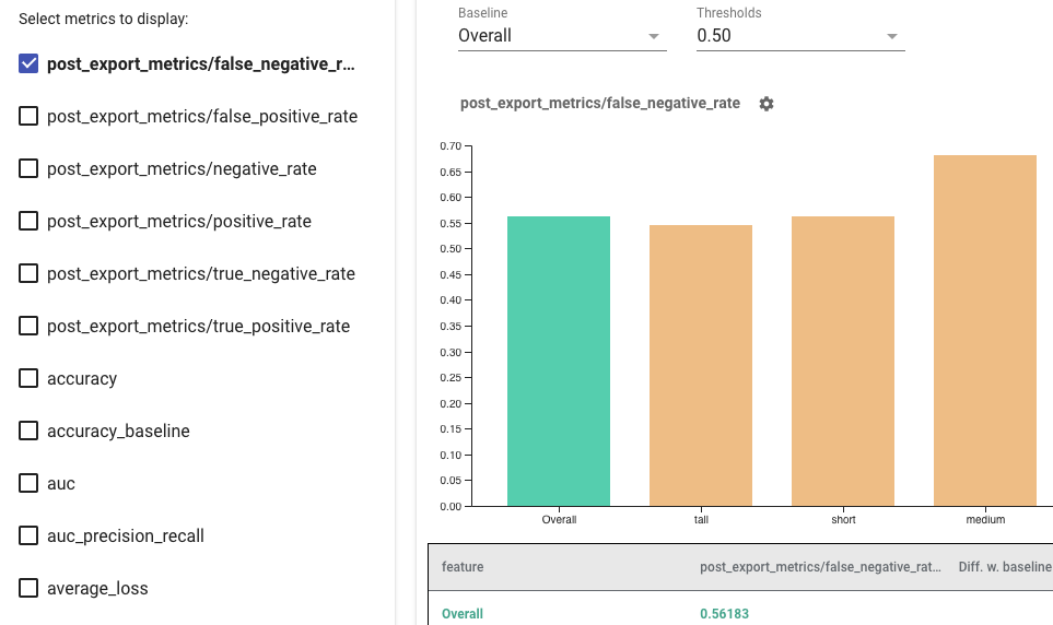
Figure 1: A snapshot of the fairness indicator tool recently launched in Tensorflow.

The absence of a unique metric capturing algorithmic fairness is not just a theoretical obstacle, it can result in troublesome dilemma in practice. An illuminating example is the analysis of the COMPAS tool for predicting recidivism by Angwin et al. (2019). The authors showed that, among black defendants who do not recidivate, the tool predicted incorrectly at twice the rate than it did for white defendants who did not recidivate. In other words, the tool was unfair according to the false positive rate metric. The creator of the tool, Northpointe, responded by demonstrating that the tool was fair according to other natural measures such as AUC (Area Under the ROC Curve). Later work showed that this tension is inherent and that it is often impossible to simultaneously satisfy multiple seemingly natural fairness criteria (Kleinberg et al., 2017) (see also discussion by Feller et al. (2016)).

Thus, there is no single generally accepted definition of fairness. Moreover, while algorithms tailored to a specific metric would be effective at first, experience shows that they become unrealistic over time: once a system is deployed and it interacts with the environment and its end-users, hidden biases encoded in the system design emerge, which in turn raise fairness complaints from new user groups and metrics originally not accounted for. This suggests working with multiple fairness criteria. However, as already pointed out, some criteria cannot be simultaneously satisfied.

To deal with the issues just discussed, we propose a data-driven model of fairness resolution guided by the unfairness complaints received, rather than by a single static definition of individual or group fairness: at each time step, a fairness resolution algorithm chooses to fix a criterion, thereby unfixing incompatible criteria, incurring a fixing cost, as well as some loss due to a new sequence of fairness complaints received. The fixing cost depends on the criterion. For instance, addressing differences in false positive rates might require augmenting the loss with a new regularization term, whereas complying with a specific individual fairness criterion could require collecting more data and learning an accurate distance metric among individuals. The objective of the fairness resolution algorithm is to minimize its cumulative loss over the course of multiple interactions with the environment.

To illustrate our model, consider the fairness indicator tool recently launched in TensorFlow (Figure 1). Using this tool, one can monitor the performance of the current classifier according to different fairness metrics. As more data is collected and the system interacts with the environment, the cost incurred by the system on each metric is updated. This cost encodes quantitative measures such as the number of data points violating a metric, as well as more qualitative ones such as the negative publicity generated as a result of violating a fairness criterion, or its legal and ethical ramifications. As these costs are updated, the system designer is faced with a choice of which metrics to prioritize at a particular time. Our goal in this work is to propose a model and algorithmic solutions to make near optimal choices in such scenarios.

In Section 2, we define our model in more detail. Our model supports multiple fairness criteria and takes into account their potential incompatibilities. We consider both a stochastic and an adversarial setting. In the stochastic setting (Section 3), we show that our framework can be naturally cast as a Markov Decision Process with stochastic losses, for which we give efficient vanishing regret algorithmic solutions. In the adversarial setting (Section 4), we describe algorithms with competitive ratio guarantees. We also report the results of experiments (Section 5) with our algorithms to demonstrate their effectiveness empirically.

2 Fairness Resolution Model

We consider the problem of resolving fairness issues in the presence of multiple fairness criteria. Not all fairness criteria can be satisfied simultaneously. The constraints can be specified by an undirected graph ${\mathscr{G}}=(V,E)$, where each vertex represents a fairness criterion and where an edge between vertices $v_{i}$ and $v_{j}$ indicates that criteria $v_{i}$ and $v_{j}$ cannot be simultaneously satisfied. We will denote by $V=\{v_{1},\ldots,v_{k}\}$ the set of $k$ fairness criteria considered. Figure 2 illustrates these definitions. Note, that vertices may represent joint criteria as in Figure 2(b).

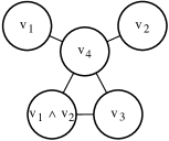
(a)	(b)

Figure 2: (a) Illustration of constraints graph ${\mathscr{G}}$. $v_{1},v_{2},v_{3},v_{4}$ represent $4$ different fairness criteria. (b) More generally, each vertex can represent a joint fairness criterion, for example $v_{1}\wedge v_{2}$. This helps specify joint constraints such as the following: $v_{1}$, $v_{2}$, and $v_{3}$ cannot be simultaneously satisfied.

At any time, a vertex $v_{i}$ can be either fixed, meaning that criterion $v_{i}$ is met or is not violated, or unfixed, meaning the opposite. Fixing criterion $v_{i}$ entails an algorithmic and resource allocation cost that we denote by $c_{i}$. Depending on the type of criterion and intervention, $c_{i}$ may include different costs, such as that of additional data collection, the average number of human hours needed to address the fairness violation, or the loss incurred in some metric, such as accuracy. Initially, all vertices are in an unfixed state. At each time step, a fairness resolution system or algorithm selects some action, which may be to fix some unfixed vertex $v_{i}$, thereby incurring the cost $c_{i}$ and unfixing any vertex adjacent to $v_{i}$, or the algorithm may select the null action, not to fix or unfix any vertex, and wait to collect more data.

In response to its action, the system receives a sequence of fairness complaints. The complaints affect one or several vertices of ${\mathscr{G}}$ and result in a fairness loss corresponding to the vertices affected. The objective of the algorithm is to minimize the total cost incurred over a period of time, which includes the total fairness loss accrued as well as the total cost of fixing various fairness criteria over that time period.

As an example, in the context of the COMPAS controversy discussed in the previous section, fixing the criteria corresponding to the false positive metric may result in an increase of the complaints related to say a calibration metric. The decision to fix a fairness criterion may also have positive implications for other metrics. For instance, criteria such as the false positive rate are correlated with accuracy and hence fixing one can be expected to decrease the complaints for the other.

Realizability. While the focus of our study is mainly theoretical and algorithmic, we wish to emphasize that our model can indeed be realized in practice. Graph ${\mathscr{G}}$ can be derived from analyzing past fairness complaints and by measuring how fixing one criterion affects the performance on others. The assignment of a complaint to one or more fairness criteria can be achieved by making use of known unfair classifiers, as discussed in Section 1, or via a multi-class multi-label classifier trained on past data. Finally, the average fixing cost specific to each criterion can be estimated from past experience. Our model also provides the flexibility of accounting for incompatibilities among more than two criteria such as those discussed by Kleinberg et al. (2017) and Feller et al. (2016). This can be achieved by augmenting the graph with vertices representing joint criteria as in Figure 2(b). The graph in that example stipulates in particular that $v_{1}$, $v_{2}$ and $v_{3}$ cannot be all simultaneously satisfied.

Ethical implications. It is worth discussing various aspects of our model and questioning its social implications, in particular its potential impact on social values of fairness and equity. There is no generally agreed upon definition of these terms, let alone a computational one. A key motivation behind the design of our model is precisely to refrain from proposing yet another definition of fairness, accepted by some, rejected by others. Indeed, experience shows that the notion of fairness is difficult to define. No two individuals seem to share the same notion of fairness, perhaps because of their distinct personal interests. Similarly, definitions of group fairness favoring some protected groups seem not to be agreed upon by other social groups. Additionally, hidden unfairness effects have been shown to come up as a result of seemingly natural notions of group fairness. Moreover, while discrimination based on given sensitive attributes is illegal by law in many countries, the notion of protected group is not well defined. In fact, in practice, reactions to a deployed software system reveal new social groups defined by more complex attributes than standard protected groups defined via standard attributes such as race, gender, ethnicity, or income level.

Instead of a static definition of fairness, we advocate a dynamic definition determined by user reactions to the system. This is further motivated by the fact that complying with multiple fairness criteria might be impossible. There may be a better chance, however, for abiding with multiple criteria over time. Our model thus avoids committing to a single dogmatic definition. However, it is also subject to some drawbacks. First, a static definition of fairness may be more convenient from the point of view of regulators. Second, while we seek not to commit to a single notion of fairness, we are in fact relying on multiple fairness criteria, which may include those typically adopted in the past. It is our hope though that the use of multiple criteria can help limit hidden biases and that, by virtue of taking into consideration the reactions to the system, our model is more democratic or flexible, and thus a more suitable candidate for regulations too.

In the next sections, we study the computational and algorithmic aspects of our model both in the stochastic and the adversarial setting. We will present nearly optimal algorithmic solutions for both settings. Our analysis will further demonstrate the flexibility of our model.

3 Stochastic Setting

In this section, we discuss a stochastic setting of our model that can be naturally described in terms of a Markov Decision Process (MDP). Next, we present algorithms with strong regret guarantees for this setting.

3.1 Description

A key observation in this scenario is that, at any time, the distribution of fairness complaints received by the system is a function of its current state, that is the current set of fixed or unfixed criteria $v_{i}$. Thus, we consider an MDP with a state space ${\mathscr{S}}\subseteq\{0,1\}^{k}$ representing the set of bit vectors for criteria: a state $s\in\{0,1\}^{k}$ is defined by $s(i)=0$ when criterion $v_{i}$ is unfixed and $s(i)=1$ when it is fixed. By definition of the incompatibility graph ${\mathscr{G}}$, $s$ is a valid state iff the set of fixed criteria at $s$ form an independent set of ${\mathscr{G}}$. When in state $s\in{\mathscr{S}}$, the system incurs a loss $\ell_{i}^{s}$ due to complaints related to criterion $i\in[k]$. $\ell_{i}^{s}$ is a random variable assumed to take values in $[0,B]$ with mean $\mu_{i}^{s}$.

The set of actions for our MDP is ${\mathscr{A}}=\{0,1,\ldots,k\}$ where a non-zero action $i$ corresponds to fixing criterion $i$, while action $0$ is the null action, that is no criterion is fixed. Transitions are deterministic: given state $s$ and action $i\in{\mathscr{A}}$, the next state is $s$ if $i=0$ since the fixed-unfixed bits for criteria are unchanged; otherwise, for $i\neq 0$ the next state is the state $s^{\prime}$ that only differs from $s$ by $s^{\prime}(i)=1$ and (possibly) $s^{\prime}(j)=0$ for all $j\in N(i)$, where $N(i)$ denotes the set of neighbors of $v_{i}$ in ${\mathscr{G}}$, since vertices neighboring $i$ must be unfixed once $i$ is fixed.

Each action $a=i$ admits a fixing cost $c_{i}$. The cost for the null action is $c_{0}=0$. The loss incurred by the algorithm when taking action $a$ at state $s$ is the sum of the fixing cost $c_{a}$ and the complaint losses at the (possibly) next state $s^{\prime}$: $\lambda(s,a)=c_{a}+\sum_{i=1}^{k}\ell_{i}^{s^{\prime}}$. The expected loss of transition $(s,a,s^{\prime})$ is thus:

$$\operatorname*{\mathbb{E}}\left[c_{a}+\sum_{i=1}^{k}\ell_{i}^{s^{\prime}}\right]=c_{a}+\sum_{i=1}^{k}\mu_{i}^{s^{\prime}}.$$ (1)

Note, $c_{a}$ and the losses $\ell_{i}^{s^{\prime}}$ are observed by the algorithm, but the mean values $\mu_{i}^{s^{\prime}}$ are unknown. To keep the formalism simple we assume that the cost $c_{a}$ of taking an action $a$ is independent of the current state $s$. However, our theoretical results easily extend to the setting where taking an action in different states has different costs. Figure 3 illustrates our stochastic MDP model in the special case of a fully connected graph ${\mathscr{G}}$, that is one where all three criteria are mutually incompatible.

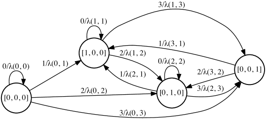
Figure 3: Illustration of the MDP for a fully connected incompatibility graph ${\mathscr{G}}$ over three criteria. The state set is ${\mathscr{S}}=\{\bm{0}=[0,0,0],\bm{1}=[1,0,0],\bm{2}=[0,1,0],\bm{3}=[0,0,1]\}$ and the action set ${\mathscr{A}}=\{0,1,2,3\}$. Each transition is labeled with $a/\lambda(s,a)$, where $a$ is the action taken from state $s$ and where $\lambda(s,a)$ is the total loss incurred as a result of the action.

Correlation sets.

In practice, the distribution of complaints related to a criterion $v_{i}$ at two different states may be related. To capture these correlations in a general way, we assume that a collection $\mathcal{C}$ of correlation sets $\mathcal{C}=\{{\mathscr{C}}_{1},{\mathscr{C}}_{2},\dots,{\mathscr{C}}_{n}\}$ is given, where each ${\mathscr{C}}_{j}$ has size at most $m$. Notice that the number of sets in $\mathcal{C}$ is at most $\binom{k}{\leq m}$. Each set ${\mathscr{C}}_{j}$ is a subset of the set of criteria $\{1,\ldots,k\}$ and results from local dependencies among the criteria it includes. We assume that at a given state $s$, each set ${\mathscr{C}}_{j}$ generates losses with mean value $\theta^{s}_{j}$ per vertex, and that if two states $s$ and $s^{\prime}$ admit the same configuration for the vertices in ${\mathscr{C}}_{j}$, then they share the same parameter $\theta^{s}_{j}=\theta^{s^{\prime}}_{j}$. Given a criterion $i$ and a state $s$, we assume that the loss incurred by criterion $i$ equals the sum of the individual losses due to each correlation set ${\mathscr{C}}_{j}$ that contains $i$. Thus, $\mu^{s}_{i}$ can be expressed as follows:

$$\mu^{s}_{i}=\sum_{j=1}^{n}\theta^{s}_{j}\operatorname{\mathbbm{1}}(i\in{\mathscr{C}}_{j}).$$ (2)

Since for each $j\in[n]$, there are at most $2^{m}$ different configurations for the vertices of ${\mathscr{C}}_{j}$ in a state $s$, there are at most $2^{m}n$ distinct parameters $\theta^{s}_{j}$. Let $\bm{\theta}$ denote the vector of all distinct parameters $\theta^{s}_{j}$. Our MDP model can then be denoted $\text{MDP}({\mathscr{S}},{\mathscr{A}},\mathcal{C},\bm{\theta})$.

3.2 Algorithm

We consider an online algorithm that at each time $t$ takes action $a_{t}$ from state $s_{t}$ of the MDP previously described and reaches state $s_{t+1}$, starting from the initial state $(0,\ldots,0)$. For standard MDP settings, the objective of an algorithm can be formulated as that of learning a policy, that is a mapping $\pi\colon{\mathscr{S}}\to{\mathscr{A}}$, with a value as close as possible to that of the optimal. Here, we are mainly interested in the cumulative loss of the algorithm over the course of $T$ interactions with the environment. Thus, the objective of an algorithm $\mathcal{A}$ can be formulated as that of minimizing its pseudo-regret, defined by

$$\operatorname*{\mathsf{Reg}}(\mathcal{A})=\sum_{t=1}^{T}\operatorname*{\mathbb{E}}\Big{[}\lambda_{t}(s_{t},a_{t})\Big{]}-\sum_{t=1}^{T}\operatorname*{\mathbb{E}}\Big{[}\lambda_{t}(s^{\pi^{*}}_{t},\pi^{*}(s^{\pi^{*}}_{t}))\Big{]},$$ (3)

where $\lambda_{t}(s,a)$ is the total loss incurred by taking action $a$ at state $s$ at time $t$ and where $s_{1}=(0,\ldots,0)$ and $\pi^{*}$ is the optimal policy. The expectation is over the random generation of the complaint losses. Given the correlation sets and the parameter $\bm{\theta}$, the optimal policy $\pi^{*}$ corresponds to moving from the initial state $(0,\ldots,0)$ to the state $s^{*}\in{\mathscr{S}}$ with the most favorable distribution and remaining at $s^{*}$ forever. We define by $g(s)$ the expected (per time step) loss incurred by staying in state $s$, i.e.,

$$g(s)\coloneqq\sum_{i=1}^{k}\mu^{s}_{i}.$$ (4)

Then given the parameters of the MDP the optimal state $s^{*}$ is defined as follows:

$$s^{*}=\operatorname*{argmin}_{s\in{\mathscr{S}}}g(s).$$ (5)

Note, in this definition of $s^{*}$, we are disregarding the one-time cost of moving to a state from the initial state, since in the long run the expected cost incurred by staying at a given state governs the choice of the optimal state.

Since our problem can be formulated as that of learning with a deterministic MDP with stochastic losses, we could seek to adopt an existing algorithm for that problem. However, the running-time complexity of such algorithms would directly depend on the size of the state space ${\mathscr{S}}$, which here is exponential in $k$, and that of the action set ${\mathscr{A}}$. Furthermore, the regret guarantees of these algorithms would also depend on $|{\mathscr{S}}||{\mathscr{A}}|$. Instead, we will show that, by exploiting the structure of the MDP, we can design vanishing regret algorithms with a computational complexity that is only polynomial in $k$ and the number of parameters. More specifically, we assume access to an oracle that can return the best state, given the estimated parameters $\bm{\theta}$, that is one that returns the solution of the optimization (5). This optimization problem is NP-hard even when correlation sets admit a simple structure.

As an example, consider the case where the correlation sets are reduced to singletons ($m=1$), ${\mathscr{C}}_{i}=\{v_{i}\}$, the loss distributions corresponding to each criterion are mutually independent. In that case, given the parameters, finding the optimal state corresponds to solving a weighted vertex cover problem for which an approximately optimal solution can be found in polynomial time. Furthermore, the true parameters of the model can be estimated accurately by observing at most $k+1$ specific states in ${\mathscr{S}}$. See Theorem 6 in Appendix A.

Case $m=2$.

To illustrate the ideas behind our general algorithm, we first consider a simpler setting where correlation sets are defined on subsets of size at most two. This setting also captures an important case where fixing a particular criterion affects the rate of fairness complaints of its neighbors. The algorithmic challenge we face here is to avoid exploring the exponentially many states in the MDP. Instead we will design an algorithm that spends an initial exploration phase by visiting a specific subset of at most $4n$. This subset denoted by ${\mathscr{K}}$, that we call as the cover of $\mathcal{C}$ will help the algorithm estimate the expected loss of any state in the MDP given the estimates of losses for states in the cover. After the exploration phase, the algorithm creates an estimate $\hat{\bm{\theta}}$ of the true parameter vector $\bm{\theta}$, uses the optimization oracle for solving (5) to find a near optimal state $\hat{s}$ and selects to stay at state $\hat{s}$ for the remaining time steps.

We next formally define the notion of a cover. For two criteria $i,j$ and $b\in\{0,1\}$, we say that $(i,j,b)$ is a dichotomy if there exist two states $s,s^{\prime}\in{\mathscr{S}}$ such that: (1) $s(j)=0$ and $s^{\prime}(j)=1$, and (2) $s(i)=s^{\prime}(i)=b$. We call the two states $s,s^{\prime}$ an $(i,j,b)$-pair. Note that if an edge $(v_{i},v_{j})$ is present in ${\mathscr{G}}$, then $(i,j,1)$ cannot be a dichotomy, since criteria $i$ and $j$ cannot be fixed simultaneously. A cover ${\mathscr{K}}$ of $\mathcal{C}$ is simply a subset of the states in the MDP that contains an $(i,j,b)$-pair for every $\{i,j\}\in\mathcal{C}$ and valid dichotomy $(i,j,b)$. Furthermore, for every singleton set $\{i\}$ in $\mathcal{C}$, the cover ${\mathscr{K}}$ contains states $s,s^{\prime}$ such that $s(i)=0,s^{\prime}(i)=1$ and $s(j)=s^{\prime}(j)$ for all $j\neq i$. Note that we only need the cover to contain an $(i,j,b)$-pair if $\{i,j\}$ is a correlation set. Hence, it is easy to see that when $m=2$, there is always a cover of size at most $4n$ in the worst case.

Next, we state our key result showing that, given the loss values for the states in a cover, we can accurately estimate the loss values for any vertex in any other state. The proof is in Appendix A.

Theorem 1.

Let ${\mathscr{K}}$ be a cover for $\mathcal{C}$. Then, for any state $s\in{\mathscr{S}}$ and any $i\in[k]$ with $s(i)=b$, we have:

$$\mu_{i}^{s} =\mu_{i}^{s^{\prime}}+\sum_{j=1}^{k}X^{i,j}_{b}\left[\operatorname{\mathbbm{1}}(s(j)=1)\operatorname{\mathbbm{1}}(s^{\prime}(j)=0)-\operatorname{\mathbbm{1}}(s(j)=0)\operatorname{\mathbbm{1}}(s^{\prime}(j)=1)\right],$$ (6)

where $s^{\prime}$ is any state in ${\mathscr{K}}$ with $s^{\prime}(i)=b$, and for $\{i,j\}\in\mathcal{C}$, $X^{i,j}_{b}\coloneqq\mu_{i}^{s_{1}}-\mu_{i}^{s_{2}}$ where $(s_{1},s_{2})$ is some $(i,j,b)$ pair. If $\{i,j\}\notin\mathcal{C}$, we define $X^{i,j}_{b}$ to be zero.

Based on the above theorem we describe our online algorithm in Figure 4 and the associated regret guarantee in Theorem 2. The proof can be found in Appendix A.

Input: The graph ${\mathscr{G}}$, correlation sets $\mathcal{C}$, fixing costs $c_{i}$. 1. Pick a cover ${\mathscr{K}}=\{s_{1},s_{2},\dots,s_{r}\}$ of $\mathcal{C}$. 2. Let $N=10\frac{T^{2/3}(\log rkT)^{1/3}}{r^{2/3}}$. 3. For each state $s\in{\mathscr{K}}$ do: • Move from current state to $s$ in at most $k$ time steps. • Play action $a=0$ in state $s$ for the next $N$ time steps to obtain an estimate $\widehat{\mu}_{i}^{s}$ for all $i\in[k]$. 4. Using the estimated losses for the states in ${\mathscr{K}}$ and Equation (6), run the oracle for the optimization (5) to obtain an approximately optimal state $\hat{s}$. 5. Move from current state to $\hat{s}$ and play action $a=0$ from $\hat{s}$ for the remaining time steps.

Figure 4: Online algorithm for $m=2$ achieving $\tilde{O}(T^{2/3})$ pseudo-regret.

Theorem 2.

Consider an $\text{MDP}({\mathscr{S}},{\mathscr{A}},\mathcal{C},\bm{\theta})$ with losses in $[0,B]$, a maximum fixing cost $c$, and correlations sets of size at most $m=2$. Let ${\mathscr{K}}$ be a cover of $\mathcal{C}$ of size $r\leq 4n$, then, the algorithm of Figure 4 achieves a pseudo-regret bounded by $O(kr^{1/3}(c+B)(\log rkT)^{1/3}T^{2/3})$. Furthermore, given access to the optimization oracle for (5), the algorithm runs in time polynomial in $k$ and $n=|\mathcal{C}|$.

The algorithm for the case of $m=2$ naturally extends to arbitrary correlation set sizes via appropriately extending the notion of a dichotomy and a cover with the size of the cover ${\mathscr{K}}$ bounded by $n2^{mn}$ in the worst case. See the Algorithm in Figure 11 in Appendix A. This leads to the following general guarantee.

Theorem 3.

Consider an $\text{MDP}({\mathscr{S}},{\mathscr{A}},\mathcal{C},\bm{\theta})$ with losses bounded in $[0,B]$ and maximum cost of fixing a vertex being $c$. Given correlations sets $\mathcal{C}$ of size at most $m$, and a cover ${\mathscr{K}}$ of $\mathcal{C}$ of size $r\leq n2^{mn}$, the algorithm in Figure 11 achieves a pseudo-regret bounded by $O(kr^{1/3}(c+B)(\log rkT)^{1/3}T^{2/3})$. Furthermore, given access to the optimization oracle for (5), the algorithm runs in time polynomial in $k$, $n=|\mathcal{C}|$ and $r=|{\mathscr{K}}|$.

3.3 Beyond $T^{\frac{2}{3}}$ regret.

In this section, we present algorithms for our problem that achieve $\tilde{O}(\sqrt{T})$ regret, first in the case $m=1$, next for any $m$, under the natural assumption that each criterion does not participate in too many correlations sets. Let us first point out that although our problem can be cast as an instance of the stochastic multi-armed bandit problem with switching costs, and arms corresponding to the states in the MDP, existing algorithms (Cesa-Bianchi et al., 2013; Simchi-Levi and Xu, 2019) achieving $\tilde{O}(\sqrt{T})$ have time complexity that depends on the number of arms which in our case is exponential ($2^{k}$). We will show here that, in most realistic instances of our model, we can achieve $\tilde{O}(\sqrt{T})$ regret efficiently.

When correlation sets are of size one, the parameter vector ${\bm{\theta}}$ can be described using the following $2k$ parameters: for each $i\in[k]$, let $\gamma^{0}_{i}$ denote the expected loss incurred by criterion $i$ when it is unfixed and $\gamma^{1}_{i}$ its expected loss when it is fixed. Our proposed algorithm is similar to the UCB algorithm for multi-armed bandits Auer et al. (2002) and maintains optimistic estimates of these parameters. We show that using the estimates of the $2k$ parameters one can construct optimistic estimates for the loss at any given state of the MDP.

For every vertex $i$, we denote by $\tau^{0}_{i,t}$ the total number of time steps up to $t$ (including $t$) during which the vertex $v_{i}$ is in an unfixed position and by $\tau^{1}_{i,t}$ the total number of times steps up to $t$ during which $v_{i}$ is in a fixed position. Fix $\delta\in(0,1)$ and let $\hat{\gamma}^{b}_{i,t}$ be the empirical expected loss observed when vertex $v_{i}$ is in state $b$, for $b\in\{0,1\}$. Our algorithm maintains the following optimistic estimates

$$\tilde{\gamma}^{b}_{i,t}=\hat{\gamma}^{b}_{i,t}-10B\sqrt{\frac{\log(kT/\delta)}{\tau^{b}_{i,t}}}.$$ (7)

To minimize the fixing cost incurred when transitioning from one state to another, our algorithm works in episodes. In each episode $h$, the algorithm first uses the current optimistic estimates to query the optimization oracle and determine the current best state $s$. Next, it remains at state $s$ for $t(h)$ time steps before querying the oracle again. The number of time steps $t(h)$ will be chosen carefully to avoid incurring the fixing costs too often. The algorithm is described in Figure 5. We will prove that it benefits from the following regret guarantee.

Input: graph ${\mathscr{G}}$, correlation sets $\mathcal{C}$, fixing costs $c_{i}$. 1. Let ${\mathscr{K}}$ be the cover of size $k+1$ that includes the all zeros state and the states corresponding to indicator vectors of the $k$ vertices. 2. Move to each state in the cover once and update the optimistic estimates according to (7). 3. For episodes $h=1,2,\dots$ do: • Run the optimization oracle (5) with the optimistic estimates as in (7) to get a state $s$. • Move from current state to state $s$. Stay in state $s$ for $t(h)$ time steps and update the corresponding estimates using (7). Here $t(h)=\min_{i}\tau^{s(i)}_{i,t_{h}}$ and $t_{h}$ is the total number of time steps before episode $h$ starts.

Figure 5: Online algorithm for $m=1$ with $\tilde{O}(\sqrt{T})$ regret.

Theorem 4.

Consider an $\text{MDP}({\mathscr{S}},{\mathscr{A}},\mathcal{C},\bm{\theta})$ with losses bounded in $[0,B]$ and maximum cost of fixing a vertex being $c$. Given correlations sets $\mathcal{C}$ of size one, the algorithm of Figure 5 achieves a pseudo-regret bounded by $O(k^{2}(c+B)^{2}\sqrt{T}\log T)$. Furthermore, given access to the optimization oracle for (5), the algorithm runs in time polynomial in $k$.

The algorithm of Figure 5 can be extended to higher $m$ values, assuming that each vertex does not participate in too many correlation sets. The guarantee associated with our general algorithm (see Figure 13 in Appendix A) leads to the following important corollary.

Corollary 1.

If ${\mathscr{G}}$ is a constant degree graph with correlation sets consisting of subsets of edges in ${\mathscr{G}}$, then there is a polynomial time algorithm that achieves a pseudo-regret bounded by $O(k^{6}(c+B)^{2}\sqrt{T}\log T)$.

4 Adversarial Setting

In the previous section, we studied a stochastic model for arrival of complaints and designed no regret algorithms. In this section, we study the setting when we cannot make assumptions about the arrival of complaints. In particular, we study an adversarial model where at each time step multiple complaints arrive for the vertices in ${\mathscr{G}}$ via the choice made by an oblivious adversary. For a given vertex $v_{i}$ and time step $t$, we denote by $\ell_{i(t)}$ the loss incurred if criterion $v_{i}$ is unfixed at time $t$. Similar to the setting from the previous section, initially all the vertices in ${\mathscr{G}}$ are in unfixed state and each vertex has a fixing cost of $c_{i}$. At each time step the algorithm can decide to fix a particular vertex. As a result all its neighbors get unfixed. At time step $t$, if criterion $v_{i}$ is unfixed then the the algorithm incurs a loss of $\ell_{i(t)}$. If $v_{i}$ is fixed at time step $t$ then algorithm incurs no loss. The overall loss incurred by the algorithm is the total fixing cost and the total loss incurred over the arrival complaints. As before, we will denote a configuration of the vertices in ${\mathscr{G}}$ using a vector $s\in\{0,1\}^{k}$ with $s(i)=0$ representing an unfixed vertex. For an algorithm $\mathcal{A}$ processing the request sequence, During the course of $T$ time steps, the total loss of processing the complaints is

$$\text{Loss}(\mathcal{A})=\sum_{i=1}^{k}\sum_{t=1}^{T}\ell_{i(t)}\cdot\operatorname{\mathbbm{1}}(s_{t}(i)=0)+\sum_{i=1}^{k}\sum_{t=2}^{T}c_{i}\cdot\operatorname{\mathbbm{1}}(s_{t-1}(i)=0,s_{t}(i)=1).$$ (8)

Define OPT to be the algorithm that given the entire loss sequence in advance, makes the optimal choice of decisions to fix vertices. Following standard terminology we define the competitive ratio of an algorithm $\mathcal{A}$ to be the maximum of $\text{Loss}(\mathcal{A})/\text{Loss}(\text{OPT})$ over all possible complaint sequences. We will design efficient online algorithms for processing the complaints that achieve a constant competitive ratio. Notice that in this setting, in order for the competitive ratio to be finite, we need to bound the range of the losses and the fixing costs of the vertices. We will assume that the cost of fixing each vertex is at least one and as before assume that the losses are bounded in the range $[0,B]$. For ease of exposition, in the rest of the discussion we will assume that at each time step complaints arrive for one of the vertices in ${\mathscr{G}}$. A simple reduction shows that an algorithm that is competitive with OPT in this setting remains so in the general setting with the same competitive ratio. We discuss this at the end of the section. Via this reduction we can consider the loss sequence to be of the form $((i_{1},\ell_{i_{1}}),\dots,(i_{T},\ell_{i_{T}}))$ where $i_{t}$ is the index of the criterion for which the $t$th complaint arrives and $\ell_{i_{t}}$ is the associated loss.

To get a better understanding of the above adversarial setting, consider the case when the graph ${\mathscr{G}}$ over the criteria has no edges, i.e., there are no conflicts. In this case, given a sequence of complaints, each with unit loss value, the optimal offline algorithm that has the entire loss sequence in advance can independently make a decision for each vertex. In particular, if the total loss of the complaints incurred at vertex $v_{i}$ exceeds the fixing cost $c_{i}$ then the optimal decision is to fix the vertex $v_{i}$, and otherwise simply incur the loss from the arriving complaints. In this case the online algorithm can also simply process each vertex independently. At each vertex the algorithm is faced with the classical ski-rental problem for which there exists a deterministic algorithm that is $2$-competitive with optimal algorithm Karlin et al. (1988). For each vertex $i$, the online algorithm simply waits till a total loss of $c_{i}$ or more has been incurred on vertex $i$ and then decides to fix it. It is easy to see that the total cost incurred by this strategy is at most twice the cost incurred by OPT.

However, the above algorithm will fail miserably in the presence of conflicts in the graph ${\mathscr{G}}$. As an example consider a graph with two vertices $v_{i}$ and $v_{j}$ that are connected by an edge. Let the fixing cost of $v_{i}$ be $1$ and the fixing cost of $v_{j}$ be $C\gg 1$. Consider a sequence of complaints, each of unit loss, consisting of $C$ complaints for $v_{j}$ followed one complaint for $v_{i}$. If this sequence is repeated $T$ times the optimal offline algorithm OPT incurs a loss of $C+T$ by fixing $v_{j}$ and incurring losses due to $v_{i}$. However, the algorithm above will incur a cost of $(2C+2)T$ thereby leading to an unbounded competitive ratio. Hence, in order to achieve a good competitive ratio one must make decisions not only based on the loss incurred at the given vertex $v_{i}$, but also the status of the vertices in the neighborhood of $v_{i}$. Our main result in this section is the algorithm in Figure 6 that achieves a constant factor competitive ratio.

Input: The graph ${\mathscr{G}}$, fixing costs $c_{i}$, loss sequence $(i_{1},\ell_{i_{1}}),\dots,(i_{T},\ell_{i_{T}})$. 1. For each $i\in[k]$, initialize $\tau_{i},\kappa_{i}$ to $0$. 2. Process the complaints in sequence and for each complaint $(i,\ell_{i})$ such that $v_{i}$ is unfixed do: (a) $\tau_{i}=\tau_{i}+\ell_{i}$. (b) While $\ell_{i}>0$ and exists $j\in N(i)$ with $\kappa_{j}>0$ do: i. Set $\Delta=\min(\ell_{i},\kappa_{i})$ and reduce both $\kappa_{i}$ and $\ell_{i}$ by $\Delta$. (c) If $\tau_{i}\geq\max\big{(}c_{i},\sum_{j\in N(i)}\kappa_{j}\big{)}$ fix $v_{i}$. Set $\tau_{i}$ to $0$ and $\kappa_{i}$ to $c_{i}$. Set $\tau_{j}=0$ for all $j\in N(i)$.

Figure 6: Online algorithm for the adversarial setting.

The algorithm described in Figure 6 makes decisions based on local neighborhood information of a vertex. Intuitively, if a vertex is fixed only once or a few times in the optimal algorithm one would like to avoid fixing it too many times. In order to achieve this, each time a vertex $v_{i}$ is fixed, it adds a barrier of $\kappa_{i}=c_{i}$ to the loss any of its neighbors need to incur before getting fixed. Hence, if a vertex is connected to a lot of fixed vertices then it has a high barrier to cross before getting fixed. During the course of the algorithm each unfixed vertex is in one of the two phases. In phase one, the vertex is accumulating losses to pay for the barrier introduced by its neighbors (step 2(b) of the algorithm). In phase two, once the barrier has been crossed the vertex follows the standard ski-rental strategy independent of other vertices for making a decision as to fix or not. Notice that via step 2(b) of the algorithm, multiple neighbors of a vertex $v_{i}$ can help bring down the barrier of $c_{i}$ introduced by the action of fixing vertex $v_{i}$. This is necessary to ensure the online algorithm does not incur a large loss on a vertex by waiting too long to fix it.

As an example consider a graph ${\mathscr{G}}$ with $k$ vertices and $k-1$ edges, where vertex $v_{0}$ is the central vertex connected to every other vertex. Let the fixing cost of vertex $v_{0}$ be a large value $C$, and the fixing cost of other vertices be one. We consider a sequence of $C$ complaints, each with unit loss arriving for vertex $v_{0}$, followed by a sequence of $C$ complaints for vertex $v_{1}$ and so on. In this case the optimal offline solution incurs a loss of $C+k$ by deciding to fix every vertex except $v_{0}$. After processing $C$ complaints for $v_{0}$, the online algorithm will fix $v_{0}$ and incur a loss of $2C$. Next, during the course of processing $C$ complaints for $v_{1}$, the algorithm fixes $v_{1}$ and incurs an additional loss of $C+1$. More importantly, due to step 2(b), the barrier $\kappa_{0}$ introduced by vertex $v_{0}$ has been reduced to zero and hence the algorithm only incurs a loss of $2$ per vertex for the remaining sequence for a total loss of $3C+2k-1$. Without the presence of step 2(b) each vertex will incur a loss of $C$ leading to a large competitive ratio.

Notice that our algorithm in Figure 6 is designed for a setting where in each time step complaints arrive for a single vertex in ${\mathscr{G}}$. If multiple vertices accumulate complaints in a time step, we can simply order them arbitrarily and run the algorithm on the new sequence. Let OPT be the optimal offline algorithm according to the chosen ordering of the complaints. Let OPT’ be the optimal offline algorithm when processing multiple complaints per time step. Notice that for each time step, the loss of OPT cannot be larger than that of OPT’ since any choice available to OPT’ is available to OPT as well. Hence it is enough to design an algorithm that is competitive with OPT. In particular, we have the following theorem. The proof is in Appendix C.

Theorem 5.

Let ${\mathscr{G}}$ be a graph with fixing costs at least one. Then, the algorithm of Figure 6 achieves a competitive ratio of at most $2B+4$ on any sequence of complaints with loss values in $[0,B]$.

5 Experiments

In this section we evaluate the performance of our algorithms developed in the stochastic setting of Section 3. We consider a simulated environment where the conflict graph $\mathcal{G}$ is generated from the Erdős-Renyi model: $G(k,p)$ where we set $p=2\frac{\log k}{k}$. This ensures that with high probability $\mathcal{G}$ is connected. Next we generate correlation sets $\mathcal{C}$ consisting of pairs of vertices in $\mathcal{G}$ sampled uniformly at random. For a parameter $\alpha>0$ that we vary, we choose $\alpha k$ pairs of vertices at random and add them as correlation sets in $\mathcal{C}$. Hence on average, each vertex participates in $\alpha$ correlation sets. We also add to $\mathcal{C}$ singleton sets for each vertex in $\mathcal{G}$. The fixing cost of each vertex is samples uniformly at random in the range $[1,5]$.

Next we describe the choice of parameters governing the loss distribution of the different states in the MDP. For a correlation set $\{i\}$ of size one corresponding to vertex $v_{i}$, we sample a parameter $\gamma^{1}_{i}$ from the beta distribution $\text{Beta}(0.5,0.5)$. For a given state $s$ with $s(i)=1$, the loss generated due to $\{i\}$ is drawn from an exponential distribution with mean $\gamma^{1}_{i}$. For a given state $s$ with $s(i)=0$, the loss generated due to $\{i\}$ is drawn from an exponential distribution with mean $\lambda\gamma^{1}_{i}$, where $\lambda>1$ is a parameter that we vary. For a correlation set $\{i,j\}$ of size two, we generate two parameters $\gamma^{1,1}_{i,j}$ and $\gamma^{1,0}_{i,j}$ from the beta distribution $\text{Beta}(0.5,0.5)$ such that $\gamma^{1,0}_{i,j}>\gamma^{1,1}_{i,j}$. For a given state $s$ with $s(i)=1$ and $s(j)=1$, the loss generated due to $\{i,j\}$ is drawn from an exponential distribution with mean $\gamma^{1,1}_{i,j}$. For states where $s(i)=0$ and $s(j)=1$ or vice-versa, the loss is generated from an exponential distribution with mean $\gamma^{1,0}_{i,j}$. Finally, for states where both $s(i)=0$ and $s(j)=0$, the loss is generated from an exponential distribution with mean $\lambda\gamma^{1,0}_{i,j}$.

In general, computation of the optimal state in (5) requires time exponential in $k$. In our experiments we approximate the optimal state by a linear programming relaxation of the optimization in (5) and use the appropriately rounded linear programming relaxation solution as a proxy for the optimal state.

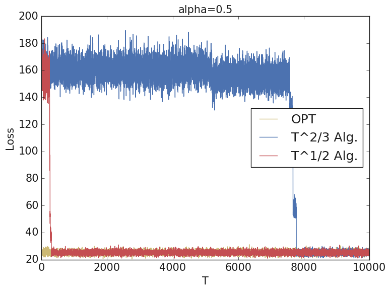
(a)

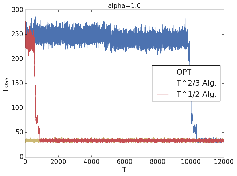
(b)

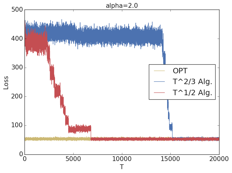
(c)

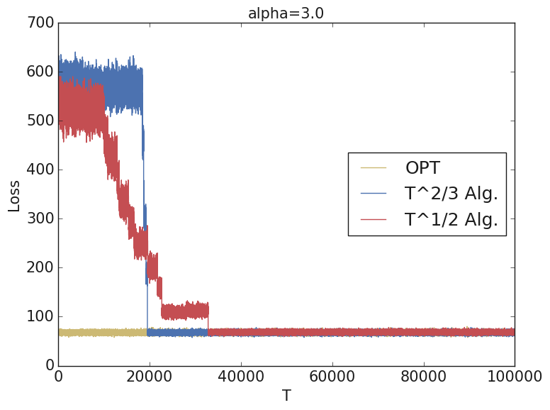
(d)

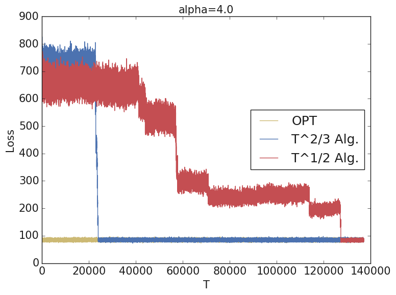
(e)

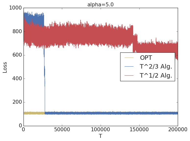
(f)

Figure 7: The figure shows the total accumulated loss incurred by the Algorithms in Figure 4 and Figure 13 on a graph with $k=50$ criteria. The parameter $\alpha$ controls the total number of correlation sets. For each value of $\alpha$, we add $\alpha k$ random pairs of vertices into correlation sets.

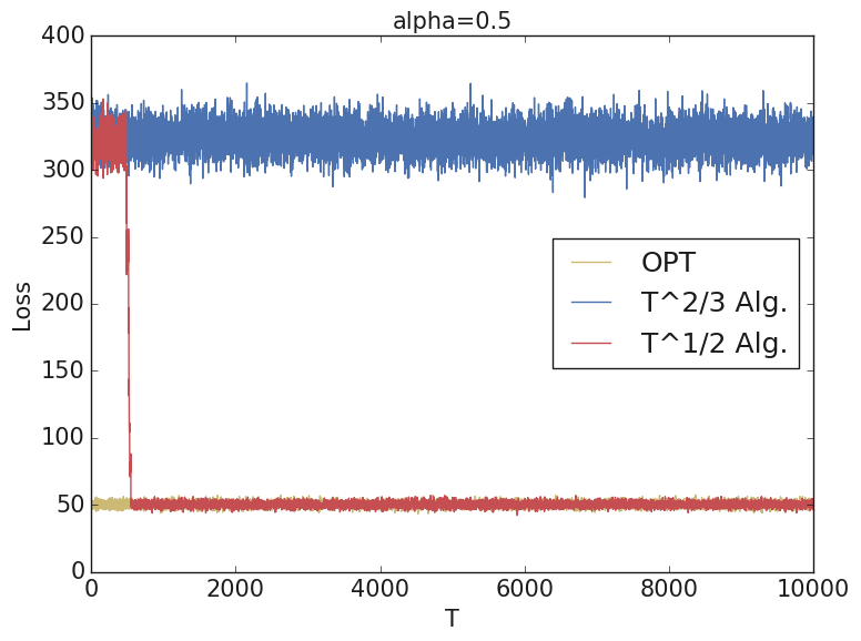
(a)

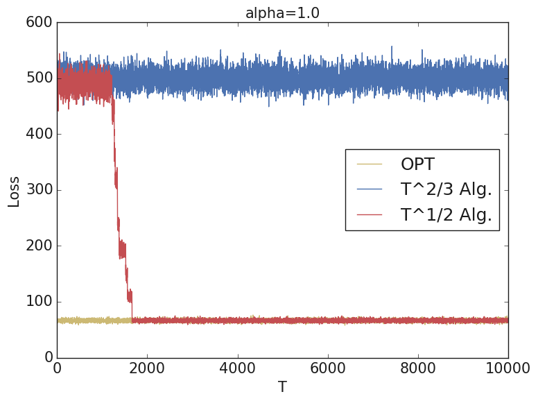
(b)

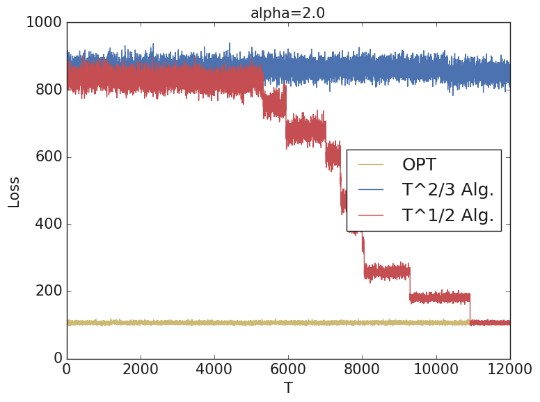
(c)

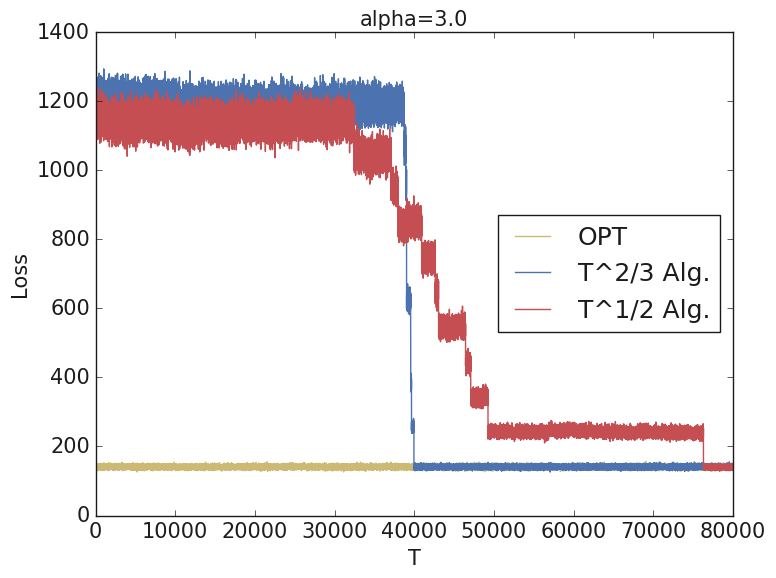
(d)

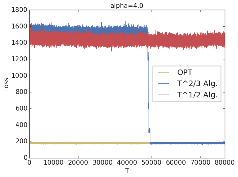
(e)

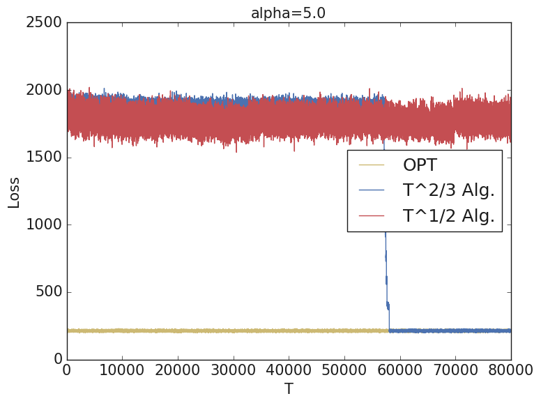
(f)

Figure 8: The figure shows the total accumulated loss incurred by the Algorithms in Figure 4 and Figure 13 on a graph with $k=100$ criteria. The parameter $\alpha$ controls the total number of correlation sets. For each value of $\alpha$, we add $\alpha k$ random pairs of vertices into correlation sets.

For general $m$, our proposed algorithms in Figure 4 and Figure 13 have complementary strengths. While the algorithm in Figure 4 incurs a higher regret as a function of the number of time steps $T$, its running time has a polynomial dependence on the parameter $\alpha$, i.e., the number of correlation sets that a vertex participates in, on average. The algorithm in Figure 13 incurs a smaller regret of $\tilde{O}(\sqrt{T})$ as a function of $T$ at the expense of an exponential dependence on $\alpha$. In Figures 7 and 8 we empirically demonstrate this behavior where for small values of $\alpha$, the $\tilde{O}(\sqrt{T})$-regret algorithm is much better, whereas for higher values of $\alpha$ the $\tilde{O}(T^{2/3})$-regret algorithm is more desirable.

For the case of $m=1$ however, i.e., singleton correlation sets, the algorithm in Figure 13 achieves a smaller regret and runs in polynomial time and hence is expected to outperform the explore-exploit based algorithm from Figure 4. As can be seen from Figure 9 this is indeed the case and the $\tilde{O}(\sqrt{T})$ regret algorithm significantly outperforms the $\tilde{O}(T^{2/3})$ regret algorithm.

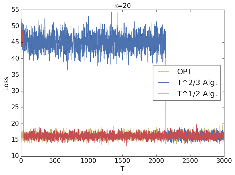
(a)

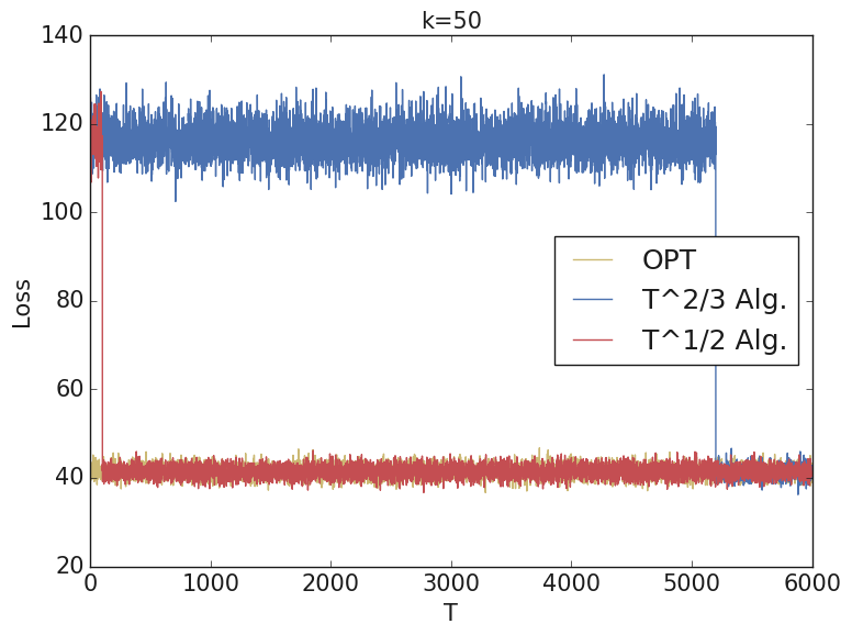
(b)

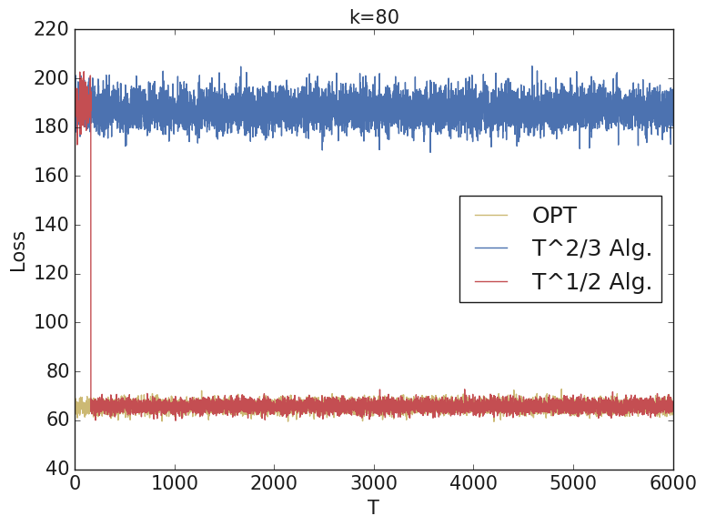
(c)

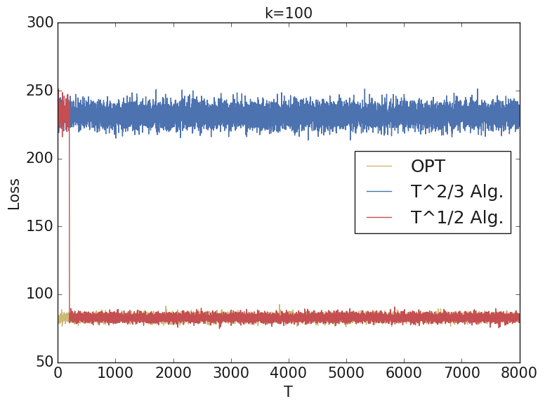
(d)

Figure 9: The figure shows the total accumulated loss incurred by the Algorithms in Figure 4 and Figure 5 for the case of $m=1$ and varying graph sizes.

6 Related Work

Much of the current research on algorithmic fairness has focused on designing solutions tailored to specific criteria such as equalized odds (Hardt et al., 2016), counterfactual or demographic parity (Kusner et al., 2017), calibration (Guo et al., 2017), or criteria for individual fairness (Zemel et al., 2013).

There has been a series of recent work on optimizing multiple fairness constraints via constrained non-convex optimization. These publications either reduce the problem to that of cost-sensitive classification (Agarwal et al., 2018; Dwork et al., 2018) or replace the non-convex constraints by convex proxies and next optimize them via external or swap regret minimization algorithms (Cotter et al., 2018b, a).

Classification has been the main focus of the research on algorithmic fairness. There has also been work, however, studying fairness criteria and algorithms for ranking (Celis et al., 2018; Beutel et al., 2019; Narasimhan et al., 2019) and clustering problems (Chierichetti et al., 2017; Schmidt et al., 2018; Backurs et al., 2019) with requirement of a proportional representation of populations within each cluster. There have been also studies of the problem of fair selection (Kearns et al., 2017; Kleinberg and Raghavan, 2018), online learning and multi-armed bandit problems (Liu et al., 2017; Joseph et al., 2018), in particular stochastic and contextual bandits (Joseph et al., 2016; Gillen et al., 2018; Gupta and Kamble, 2019) and reinforcement learning (Jabbari et al., 2017; Doroudi et al., 2017; Wen et al., 2019; Zhang and Shah, 2014), human-classifier hybrid decision systems (Madras et al., 2018), or fair personalization (Celis and Vishnoi, 2017).

There have also been studies of the inherent tension between satisfying multiple fairness metrics and composition of fair classifiers. Kleinberg et al. (2017) and Feller et al. (2016) demonstrate that it is impossible to satisfy equal opportunity and calibration at the same time. Blum et al. (2018); Dwork et al. (2018, 2020) study whether a composition of fair classifiers remains fair and provided negative results. Menon and Williamson (2018) study the accuracy vs. fairness tradeoff in classification problems with group fairness constraints.

Joseph et al. (2016) study a notion of individual fairness in the context of stochastic bandits. There are $k$ arms and in each time step, the algorithm picks an arm according to distribution $p_{t}$. For arm $i_{t}$ a stochastic reward is revealed with mean vector $\mu_{i}$. Furthermore, the authors impose the fairness constraint that at each time step $t$, the algorithm can pick an arm $i$ with higher probability than arm $j$ only if $\mu_{i}>\mu_{j}$ (with high probability).

Gillen et al. (2018) extend the stochastic bandits setting to the case of linear contextual bandits. Here, $k$ adversarially chosen context vectors $x^{t}_{1},\dots,x^{t}_{k}$ arrive at time $t$ and the mean reward of playing arm $i$ at time $t$ is $\theta\cdot x^{t}_{i}$ for an unknown vector $\theta$. The notion of individual fairness considered is that if two contexts $x^{t}_{i}$ and $x^{t}_{j}$ are close to each other, then the corresponding arms should be played with similar probabilities. More specifically, it must holds that $|p_{t}(i)-p_{t}(j)|\leq d(x^{t}_{i},x^{t}_{j})$. The distance metric $d$ is assumed to be a Mahalanobis distance with an unknown matrix $A$ and after each round it is revealed which individual fairness criteria were violated.

While we avoid using special structures of specific fairness metrics in our algorithm design, several of the studies mentioned before can be cast into our framework. There are, however, several important differences that make the algorithmic guarantees incomparable as these studies aim to design algorithms tailored to a specific metric. For instance, to model the stochastic bandit setting of Joseph et al. (2016) as described above, we could consider a graph ${\mathscr{G}}$ with $\binom{k}{2}$ vertices, one for each pair of arms. Each vertex captures the individual fairness metric associated with the pair. More importantly, the graph will have no edges. Hence, the states in the MDP can be described by a vector in $\{0,1\}^{\binom{k}{2}}$ describing which pairs of arms violate individual fairness. The actions will consist of picking a probability vector $p_{t}$ over the $k$ arms in each time step. However, in the setting of Joseph et al. (2016), the transition dynamics are unknown since fairness violations as a result of taking an action $p_{t}$ depend on the true unknown means of the arms. Since the work of Joseph et al. (2016) studies a particular fairness metric, one can use special structure of the problem to design a customized solution. In our model, we study arbitrary fairness metrics and thus, some assumptions about the transition dynamics are necessary.

Recent works have also studied the long-term impact of optimizing fairness criteria in settings with feedback mechanisms (Liu et al., 2018; Hashimoto et al., 2018; Mouzannar et al., 2019; Kannan et al., 2019). Liu et al. (2018) show that, in certain situations, constrained loss minimization to equalize certain fairness criteria could lead to further disparate impact in the long run. Hashimoto et al. (2018) proposed algorithms for minimizing such disparate impact in settings involving repeated loss minimization. More recently, Jabbari et al. (2017); Wen et al. (2019) study the problem of satisfying fairness constraints in reinforcement learning settings involving a Markov Decision Process. The authors in Jabbari et al. (2017) consider learning in an MDP where the fairness criteria requires that the algorithm never takes an action $a$ over action $a^{\prime}$ if the long-term reward is higher. It is clear to see that the optimal policy for the MDP indeed satisfies this property. Hence, there does exist a fair policy. However, the authors show that finding a near optimal fair policy requires time exponential in the size of the state space.

Wen et al. (2019) consider other fairness metrics such as demographic parity in the context of learning in MDPs. Doroudi et al. (2017) show that existing importance sampling methods for off-policy policy selection in reinforcement learning can lead to unfair outcomes and present algorithms to mitigate this effect. Zhang and Shah (2014) define a fairness solution criterion for multi-agent MDPs. The recent work of Mladenov et al. (2020) studies optimzing long term social welfare in recommender systems.

While our work also involves learning in a Markov Decision Process (MDP) and optimizing fairness in the long term, the setup and the motivation are different. Unlike all the previous work mentioned, we do not commit to a fixed definition of fairness and allow for arbitrary fairness criteria. Hence, states in our MDP correspond to the current configurations of different fairness criteria. Rather than studying each fairness metric in isolation, the objective of our work is to propose a data-driven model that can learn from feedback, a near-optimal configuration of the metrics to impose on the system. To the best of our knowledge, ours is the first work to incorporate optimizing fairness metrics of arbitrary types in an online setting. In this context, the recent work of Kearns et al. (2019) studies a specific combination of group and individual fairness metrics. The authors consider a setting where there is a distribution over individuals as well as a distribution over classification tasks. They consider algorithms for achieving average individual fairness, that is in expectation over classification tasks, the performance of the algorithm on a group fairness metric such as demographic parity should be the same for each individual.

An important aspect of our stochastic MDP-based model requires the ability to observe the losses associated with different fairness criteria at each time. This relates to the problem of evaluating (un)fairness according to different metrics from data. Many such metrics require access to both labeled data and to sensitive attribute information such as race or gender, for accurate evaluation. A recent line of work has studied this estimation problem when one has limited and/or noisy access to sensitive attribute information (Gupta et al., 2018; Coston et al., 2019; Lamy et al., 2019; Wang et al., 2020).

7 Conclusion

We presented a new data-driven model of fairness in the presence of multiple criteria, with algorithms benefitting from theoretical guarantees both in the stochastic and in the adversarial setting. While we believe that our model can be realized in practice and while our experiments show the effectiveness of our algorithms empirically, several extensions are worth exploring to further expand their applicability. These include fixing costs that can vary with time to capture the varying algorithmic price and human effort required to address various fairness criteria. Similarly, the expected losses in our stochastic model could be time-dependent to express the growing cost of a fairness criterion not being addressed.

Appendix A Stochastic Setting

We first show that in the stochastic model, if correlation sets are of size one then one can efficiently approximate the cost of the optimal state up to a factor of two.

Theorem 6.

If correlations sets are of size one ($m=1$), then, for any $\epsilon,\delta>0$, the true parameter vector for $\text{MDP}({\mathscr{S}},{\mathscr{A}},\mathcal{C},\bm{\theta})$ can be approximated to $\epsilon$-accuracy in $\ell_{\infty}$-norm with probability at least $1-\delta$, in at most $O(\frac{B^{2}k}{\epsilon^{2}}\log(\frac{k}{\delta}))$ time steps and exploring at most $k+1$ specific states in ${\mathscr{S}}$. Furthermore, given a parameter vector $\bm{\theta}$, there is an algorithm that runs in time polynomial in $k$ and finds an approximately optimal state $s^{\prime}$ such that $g(s^{\prime})\leq 2\min_{s\in{\mathscr{S}}}g(s)$.

Proof.

Notice that when correlation sets are of size one, the expected loss incurred for criterion $v_{i}$ at any given state $s$ solely depends on whether $s(i)=0$ or $s(i)=1$. Hence in this case the MDP consists of $2k$ parameters where we use $\gamma^{1}_{i}$ and $\gamma^{0}_{i}$ to denote the expected losses incurred by vertex $i$ when it is in fixed and unfixed position respectively. For any $\delta>0$, by Hoeffding’s inequality, we have that if we stay in state $s=(0,0,\dots,0)$ for $N=\frac{B^{2}}{\epsilon^{2}}\log(2k/\delta)$ time steps then with probability at least $1-\frac{\delta}{2}$, we have each $\gamma^{0}_{i}$ estimated up to $\epsilon$ accuracy. Let $e_{i}\in\{0,1\}^{k}$ denote the indicator vector for $i$. If we stay in state $s=e_{i}$ for $\frac{B^{2}}{\epsilon^{2}}\log(2k/\delta)$ time steps, then with probability at least $1-\frac{\delta}{2}$ we have $\gamma^{1}_{i}$ estimated up to $\epsilon$ accuracy. Hence, overall after $O(\frac{B^{2}k}{\epsilon^{2}}\log(\frac{k}{\delta}))$ time steps, we have each parameter estimated up to $\epsilon$ accuracy. Notice that in total we observe at most $k+1$ states.

Next we show how to efficiently approximate the loss of the best state. Given the parameters of the MDP each vertex has two costs $\Lambda^{(1)}_{i}=\gamma^{0}_{i}$, denoting the cost incurred if the vertex is unfixed and $\Lambda^{(2)}_{i}=c_{i}+\gamma^{1}_{i}$, denoting the cost incurred if the vertex is fixed. Without loss of generality assume that $\Lambda^{(1)}_{i}>\Lambda^{(2)}_{i}$ (any vertex that does not satisfy this can be safely left unfixed). For each $i$, define $y_{i}=1$ if vertex $i$ is unfixed otherwise define $y_{i}=0$. Then the offline problem of finding the best state can be written as

min $$\sum_{i=1}^{k}(1-y_{i})\Lambda^{2}_{i}+y_{i}\Lambda^{1}_{i}=\sum_{i=1}^{k}y_{i}\gamma_{i}+\sum_{i=1}^{k}\Lambda^{(2)}_{i}$$

s.t. $$y_{i}\in\{0,1\}$$

$$y_{i}+y_{j} \geq 1,\,\,\forall(v_{i},v_{j})\in E.$$

Here $\gamma_{i}=\Lambda^{(1)}_{i}-\Lambda^{(2)}_{i}>0$. By relaxing $y_{i}$ to be in $[0,1]$ and solving the corresponding linear programming relaxation, we get a solution $y^{*}_{1},y^{*}_{2},\dots,y^{*}_{k}$. Let LPval denote the linear programming objective value achieved by $y^{*}_{1},y^{*}_{2},\dots,y^{*}_{k}$. Since the linear programming formulation is a valid relaxation of the problem of finding the best state, we have $\text{LPval}\leq\min_{s\in{\mathscr{S}}}g(s)$.

We output the state $s^{\prime}$ in which a vertex $i$ if and only if $y^{*}_{i}<1/2$. Let $S$ be the set of fixed vertices. We have

$$g(s^{\prime}) =\sum_{i\in S}\Lambda^{(2)}_{i}+\sum_{i\notin S}\Lambda^{(1)}_{i}$$

$$=\sum_{i=1}^{k}\Lambda^{(2)}_{i}+\sum_{i\notin S}(\Lambda^{(1)}_{i}-\Lambda^{(2)}_{i})$$

$$=\sum_{i=1}^{k}\Lambda^{(2)}_{i}+\sum_{i\notin S}\gamma_{i}$$

$$<\sum_{i=1}^{k}\Lambda^{(2)}_{i}+2\sum_{i\notin S}y^{*}_{i}\gamma_{i}$$

$$<2\Big{(}\sum_{i=1}^{k}\Lambda^{(2)}_{i}+\sum_{i=1}^{k}y^{*}_{i}\gamma_{i}\Big{)}$$

$$<2\cdot\text{LPval}$$

$$\leq\min_{s\in{\mathscr{S}}}2g_{\bm{p}}(s).$$

∎

A.1 Case $m=2$

To illustrate the ideas behind our general algorithm, we first consider a simpler setting where correlation sets are defined on subsets of size at most two. This setting also captures an important case where fixing a particular criterion affects the rate of fairness complaints of its neighbors.

Our algorithm consists of an exploration phase where it observes the losses for a specific subset of at most $4n$ states. We will show that after the exploration phase, the algorithm can accurately estimate the expected loss for any other state $s\in{\mathscr{S}}$. Notice that the number of states in ${\mathscr{S}}$ is in general exponential in $k$. Thus, the subset of states to observe must be carefully chosen and must take into account the structure of the graph ${\mathscr{G}}$. After the exploration phase, the algorithm creates an estimate $\hat{\bm{\theta}}$ of the true parameter vector $\bm{\theta}$, uses the optimization oracle for solving (5) to find a near optimal state $\hat{s}$ and selects to stay at state $\hat{s}$ for the remaining time steps.

Let $c$ denote the maximum fixing cost: $c=\max_{i\in[k]}c_{i}$. We will show that the pseudo-regret of our algorithm is bounded by $O(k\log k(c+B)^{1/3}T^{2/3}\log(kT))$. We first describe how we select the subset of states to observe in the exploration phase.

We say that $(i,j,b)$ is a dichotomy if for two criteria $i$ and $j$ and for $b\in\{0,1\}$, there exist two states $s,s^{\prime}\in{\mathscr{S}}$ such that: (1) $s(j)=0$ and $s^{\prime}(j)=1$, and (2) $s(i)=s^{\prime}(i)=b$. Note that if an edge $(v_{i},v_{j})$ is present in ${\mathscr{G}}$, then $(i,j,1)$ cannot be a dichotomy, since criteria $i$ and $j$ cannot be fixed simultaneously.

Definition 1.

Consider a subset ${\mathscr{K}}\subset{\mathscr{S}}$. We will say that ${\mathscr{K}}$ is a cover for $\mathcal{C}$ if for any dichotomy $(i,j,b)$, where $\{i,j\}$ is a correlation set ($\{i,j\}\in\mathcal{C}$) there exist two states $s,s^{\prime}\in{\mathscr{K}}$ such that:

1. they agree in all criteria except criterion $j$: $s(l)=s^{\prime}(l)$ for all $l\neq j$;

2. criteria $i$ is in state $b$ in both: $s(i)=s^{\prime}(i)=b$;

3. we have that $s(j)=0$ and $s^{\prime}(j)=1$.

We call such a pair $(s,s^{\prime})$ an $(i,j,b)$-pair.

Furthermore, for every singleton set $\{i\}$ in $\mathcal{C}$, the cover ${\mathscr{K}}$ contains states $s,s^{\prime}$ such that $s(i)=0,s^{\prime}(i)=1$ and $s(j)=s^{\prime}(j)$ for all $j\neq i$. We can always find a cover ${\mathscr{K}}$ of size at most $4n$ by picking for each $\{i,j\}\in\mathcal{C}$, at most four states corresponding to different bit configurations for $i$ and $j$, with all other bits set to zero. For any valid dichotomy $(i,j,b)$ we define $X^{i,j}_{b}$ as

$$X^{i,j}_{b}\coloneqq\mu_{i}^{s}-\mu_{i}^{s^{\prime}},$$ (9)

where $s,s^{\prime}\in{\mathscr{K}}$ is an $(i,j,b)$ pair. If $\{i,j\}\notin\mathcal{C}$ we define $X^{i,j}_{b}$ to be zero. Notice that the values $X^{i,j}_{b}$ can be approximated from estimating the loss values of states in the cover. Next, we state our key result showing that, given the loss values for the states in a cover, we can accurately estimate the loss values for any vertex in any other state.

Theorem 1.

Let ${\mathscr{K}}$ be a cover for $\mathcal{C}$. Then, for any state $s\in{\mathscr{S}}$ and any $i\in[k]$ with $s(i)=b$, we have:

$$\mu_{i}^{s} =\mu_{i}^{s^{\prime\prime}}+\sum_{j=1}^{k}X^{i,j}_{b}\left[\operatorname{\mathbbm{1}}(s(j)=1)\operatorname{\mathbbm{1}}(s^{\prime\prime}(j)=0)-\operatorname{\mathbbm{1}}(s(j)=0)\operatorname{\mathbbm{1}}(s^{\prime\prime}(j)=1)\right],$$ (10)

where $s^{\prime\prime}$ is any state in ${\mathscr{K}}$ with $s^{\prime\prime}(i)=b$.

Proof.

Consider a correlation set $\{i,j\}$. The expected loss incurred by vertex $v_{i}$ or $v_{j}$ due to this set in any given state depends solely on the configuration of $v_{i}$ and $v_{j}$ in that state. Hence there are four parameters in the $\bm{\theta}$ vector corresponding to the correlation set $\{i,j\}$ and we denote them using $\gamma^{a,b}_{i,j}$, where $a,b\in\{0,1\}$. Let $s,s^{\prime}$ be an $(i,j,b)$ pair. When we switch from $s$ to $s^{\prime}$ the only difference in the expected losses for vertex $i$ comes from the pair $(i,j)$. Hence we have

$$\mu^{s^{\prime}}_{i}-\mu^{s}_{i} =\gamma^{b,1}_{i,j}-\gamma^{b,0}_{i,j}\coloneqq X^{i,j}_{b}.$$

Hence, given the loss estimates for states in ${\mathscr{K}}$ we can estimate $X^{i,j}_{b}$ for each $i,j\in[k]$ and $b\in\{0,1\}$. Next, given an arbitrary state $s$ with $s(i)=b$ let $s^{\prime\prime}\in{\mathscr{K}}$ such that $s^{\prime\prime}(i)=b$. We have

$$\mu^{s}_{i} =\mu^{s^{\prime\prime}}_{i}+\sum_{\begin{subarray}{c}j:s(j)=0\\ s^{\prime\prime}(j)=1\end{subarray}}(\gamma^{b,0}_{i,j}-\gamma^{b,1}_{i,j})+\sum_{\begin{subarray}{c}j:s(j)=1\\ s^{\prime\prime}(j)=0\end{subarray}}(\gamma^{b,1}_{i,j}-\gamma^{b,0}_{i,j})$$

$$=\mu^{s^{\prime\prime}}_{i}+\sum_{\begin{subarray}{c}j:s(j)=1,\\ s^{\prime\prime}(j)=0\end{subarray}}X^{i,j}_{b}-\sum_{\begin{subarray}{c}j:s(j)=0,\\ s^{\prime\prime}(j)=1\end{subarray}}X^{i,j}_{b}$$

$$=\mu_{i}^{s^{\prime\prime}}+\sum_{j=1}^{k}X^{i,j}_{b}\left[\operatorname{\mathbbm{1}}(s(j)=1)\operatorname{\mathbbm{1}}(s^{\prime\prime}(j)=0)-\operatorname{\mathbbm{1}}(s(j)=0)\operatorname{\mathbbm{1}}(s^{\prime\prime}(j)=1)\right].$$

∎

Based on the above theorem we describe our online algorithm in Figure 10 (same as the algorithm in Figure 4 of the main body) and the associated regret guarantee.

Input: The graph ${\mathscr{G}}$, correlation sets $\mathcal{C}$, fixing costs $c_{i}$. 1. Pick a cover ${\mathscr{K}}=\{s_{1},s_{2},\dots,s_{r}\}$ of $\mathcal{C}$. 2. Let $N=10\frac{T^{2/3}(\log rkT)^{1/3}}{r^{2/3}}$. 3. For each state $s\in{\mathscr{K}}$ do: • Move from current state to $s$ in at most $k$ time steps. • Play action $a=0$ in state $s$ for the next $N$ time steps to obtain an estimate $\widehat{\mu}_{i}^{s}$ for all $i\in[k]$. 4. Using the estimated losses for the states in ${\mathscr{K}}$ and Equation (10), run the oracle for the optimization (5) to obtain an approximately optimal state $\hat{s}$. 5. Move from current state to $\hat{s}$ and play action $a=0$ from $\hat{s}$ for the remaining time steps.

Figure 10: Online algorithm for $m=2$ achieving $\tilde{O}(T^{2/3})$ pseudo-regret.

Theorem 2.

Consider an $\text{MDP}({\mathscr{S}},{\mathscr{A}},\mathcal{C},\bm{\theta})$ with losses in $[0,B]$, a maximum fixing cost $c$, and correlations sets of size at most $m=2$. Let ${\mathscr{K}}$ be a cover of $\mathcal{C}$ of size $r\leq 4n$, then, the algorithm of Figure 10 (same as Figure 4) achieves a pseudo-regret bounded by $O(kr^{1/3}(c+B)(\log rkT)^{1/3}T^{2/3})$. Furthermore, given access to the optimization oracle for (5), the algorithm runs in time polynomial in $k$ and $n=|\mathcal{C}|$.

Proof.

In each time step the maximum loss incurred by any criterion is bounded by $c+B$. Let $\{s_{1},s_{2},\dots,s_{r}\}$ be the states in ${\mathscr{K}}$. During the exploration phase the algorithm stays in each state for $N$ time steps and incurs a total loss bounded by $kNr(c+B)$. During the exploration phase the algorithm moves from one state to another in at most $k$ steps and incurs a total additional loss of at most $rk^{2}(c+B)$. At any given state $s\in{\mathscr{K}}$ and vertex $v_{i}$, after $N$ time steps we will, with probability at least $1-\delta$, an estimate of $\mu^{s}_{i}$ up to an accuracy of $2B\sqrt{\frac{\log 1/\delta}{N}}$. Setting $\delta=1/(rkT^{4})$ and using union bound, we have that at the end of the exploration phase, with probability at least $1-\frac{1}{T^{4}}$, the algorithm will have estimate $\hat{\mu}^{s}_{i}$ for all $s\in{\mathscr{K}}$ and $i\in[k]$ such that

$$\hat{\mu}^{s}_{i}-\mu^{s}_{i}\leq 4B\sqrt{\frac{\log rkT}{N}}.$$ (11)

Hence during the exploitation phase, with high probability, the algorithm will have the estimate for the expected loss of each state in ${\mathscr{S}}$, i.e., $\sum_{i}\mu^{s}_{i}$ up to an error of $4kB\sqrt{\frac{\log rkT}{N}}$. Combining the above we get that the total pseudo-regret of the algorithm is bounded by

$$\operatorname*{\mathsf{Reg}}(\mathcal{A}) \leq kNr(c+B)+rk^{2}(c+B)+\Big{(}1-\frac{1}{T^{4}}\Big{)}4kBT\sqrt{\frac{\log rkT}{N}}+\frac{1}{T^{4}}k(c+B)T.$$

Setting $N=10\frac{T^{2/3}(\log rkT)^{1/3}}{r^{2/3}}$ we get that

$$\operatorname*{\mathsf{Reg}}(\mathcal{A})\leq O(kr^{1/3}(c+B)(\log rkT)^{1/3}T^{2/3}).$$

∎

A.2 General case

The algorithm for the case of $m=2$ naturally extends to arbitrary correlation set sizes. Overall the structure of the algorithm remains the same where we pick a cover of $\mathcal{C}$ and estimate the losses incurred in states that belong to the cover. Using the estimated losses we are able to approximately estimate the loss of any vertex at any other state. In order to do this we extend the definition of the cover as follows. Given correlation sets of arbitrary size in $\mathcal{C}$, a vertex $v_{i}$ may participate in many of them. We say that vertices $v_{i}$ and $v_{j}$ share a correlation set, if they appear together in a set in $\mathcal{C}$. Consider the set of indices of all the vertices that $v_{i}$ shares a correlation set with. We partition this set into disjoint subsets such that no two vertices in different subsets share a correlation set. For a given vertex $v_{i}$, we denote this collection of disjoint subsets by $I_{i}$. For example, if $\mathcal{C}$ contains sets $\{1,2\}$, $\{1,3\}$, and $\{1,4\}$, then, $I_{1}$ consists of the set $\{2,3,4\}$. On the other hand if $\mathcal{C}$ contains sets $\{1,2,3\},\{1,3,4\},$ and $\{1,6,7\}$ then, $I_{1}$ consists of sets $\{2,3,4\}$ and $\{6,7\}$. For a given state $s$ and $J\in I_{i}$ we denote by $s(J)$ the vector $s$ restricted to indices in $J$. Notice that, in the worst case, $I_{i}$ will consist of a single set of size at most $\min(k-1,nm)$. However, for more structured cases (e.g, $m=2$) we expect $I_{i}$ to consist of subsets of small sizes.

Given $i\in[k]$, $J\in I_{i}$, $b\in\{0,1\}$ and vectors ${u}_{1},{u}_{2}$, we say that $(i,b,J,{u}_{1},{u}_{2})$ is a dichotomy, if there exist two states $s,s^{\prime}\in{\mathscr{S}}$ such that: (1) $s(J)={u}_{1},s^{\prime}(J)={u}_{2}$, (2) $s(i)=b=s^{\prime}(i)$, and (3) $s,s^{\prime}$ agree in all other criteria. We call such a pair of states $s,s^{\prime}$ an $(i,b,J,u_{1},u_{2})$ pair. We next extend the definition of a cover as follows. A subset ${\mathscr{K}}\subseteq S$ is called a cover of $\mathcal{C}$ if for any valid dichotomy $(i,b,J,{u}_{1},{u}_{2})$, there exists an $(i,b,J,{u}_{1},{u}_{2})$ pair $s,s^{\prime}\in{\mathscr{K}}$. In general, we will always have a cover of size at most $n2^{mn}$. Similar to (9), for a valid dichotomy $(i,b,J,u_{1},u_{2})$, we define $X^{i,u_{1},u_{2}}_{b,J}$ as

$$X^{i,u_{1},u_{2}}_{b,J}\coloneqq\mu^{s}_{i}-\mu^{s^{\prime}}_{i},$$ (12)

where $s,s^{\prime}\in{\mathscr{K}}$ is an $(i,b,J,u_{1},u_{2})$ pair. Given the loss values in the states present in ${\mathscr{K}}$, we can estimate the loss of any other state using Theorem 7 stated below.

Theorem 7.

Let ${\mathscr{K}}$ be a cover for $\mathcal{C}$. Then, for any state $s\in{\mathscr{S}}$ and any $i\in[k]$ with $s(i)=b$, we have:

$$\mu_{i}^{s} =\mu_{i}^{s^{\prime\prime}}+\sum_{J\in I_{i}}X^{i,s(J),s^{\prime\prime}(J)}_{b,J}$$ (13)

Here $s^{\prime\prime}$ is any state in ${\mathscr{K}}$ with $s^{\prime\prime}(i)=b$.

Proof.

Let $s,s^{\prime}\in{\mathscr{K}}$ be an $(i,b,J,u_{1},u_{2})$ pair. When we move from state $s$ to $s^{\prime}$, the only difference between the expected losses incurred by vertex $v_{i}$ comes from the configuration of the vertices in $J$. Hence there at at most $2^{|J|+1}$ distinct parameters governing the expected loss incurred by vertex $i$ in a given state $s$ due to the configuration of the vertices in $J$. Denoting these parameters by $\gamma^{b,s(J)}_{i,J}$ we have

$$\mu^{s^{\prime}}_{i}-\mu^{s}_{i}=\gamma^{b,s^{\prime}(J)}_{i,J}-\gamma^{b,s(J)}_{i,J}\coloneqq X^{i,s^{\prime}(J),s(J)}_{b,J}.$$

Given the loss values for the states in the cover ${\mathscr{K}}$, we can estimate the quantities $X^{i,s(J),s^{\prime\prime}(J)}_{b,J}$.

Next, for an arbitrary state $s$ such that $s(i)=b$, let $s^{\prime\prime}\in{\mathscr{K}}$ be such that $s^{\prime\prime}(i)=b$. We have

$$\mu^{s}_{i} =\mu^{s^{\prime\prime}}_{i}+\sum_{J\in I_{i}}\gamma^{b,s(J)}_{i,J}-\gamma^{b,s^{\prime\prime}(J)}_{i,J}$$

$$=\sum_{J\in I_{i}}X^{i,s(J),s^{\prime\prime}(J)}_{b,J}.$$

∎

For general correlation sets with each vertex participating in at most $n$ sets, we use (13) instead of (10) to estimate losses in step 4 of the algorithm in Figure 10. The algorithm for general $m$ is described in Figure 11 and has the following associated regret guarantee. The proof is identical to the proof of Theorem 2.

Input: The graph ${\mathscr{G}}$, correlation sets $\mathcal{C}$, fixing costs $c_{i}$. 1. Pick a cover ${\mathscr{K}}=\{s_{1},s_{2},\dots,s_{r}\}$ of $\mathcal{C}$. 2. Let $N=10\frac{T^{2/3}(\log rkT)^{1/3}}{r^{2/3}}$. 3. For each state $s\in{\mathscr{K}}$ do: • Move from current state to $s$ in at most $k$ time steps. • Play action $a=0$ in state $s$ for the next $N$ time steps to obtain an estimate $\widehat{\mu}_{i}^{s}$ for all $i\in[k]$. 4. Using the estimated losses for the states in ${\mathscr{K}}$ and Equation (13), run the oracle for the optimization (5) to obtain an approximately optimal state $\hat{s}$. 5. Move from current state to $\hat{s}$ and play action $a=0$ from $\hat{s}$ for the remaining time steps.

Figure 11: Online algorithm for general $m$ achieving $\tilde{O}(T^{2/3})$ pseudo-regret.

Theorem 3.

Consider an $\text{MDP}({\mathscr{S}},{\mathscr{A}},\mathcal{C},\bm{\theta})$ with losses bounded in $[0,B]$ and maximum cost of fixing a vertex being $c$. Given correlations sets $\mathcal{C}$ of size at most $m$, and a cover ${\mathscr{K}}$ of $\mathcal{C}$ of size $r\leq n2^{mn}$, the algorithm in Figure 11 achieves a pseudo-regret bounded by $O(kr^{1/3}(c+B)(\log rkT)^{1/3}T^{2/3})$. Furthermore, given access to the optimization oracle for (5) the algorithm runs in time polynomial in $k$, $n=|\mathcal{C}|$ and $r=|{\mathscr{K}}|$.

Appendix B Beyond $T^{\frac{2}{3}}$ regret

In this section, we present algorithms for our problem that achieve $\tilde{O}(\sqrt{T})$ regret, first in the case $m=1$, next for any $m$, under the natural assumption that each criterion does not participate in too many correlations sets.

Let us first point out that our problem can be cast as an instance of the stochastic multi-armed bandit problem with switching costs, where each state $s$ is viewed as an arm and where the cost of transitions from state $s$ to state $s^{\prime}$ is the switching cost between $s$ and $s^{\prime}$. For the instance of this problem with identical switching costs, Cesa-Bianchi et al. [2013][Appendix A] gave an algorithm achieving expected regret $\tilde{O}(\sqrt{T})$, via an arm-elimination technique with at most $O(\log\log T)$ switches. However, naturally, the regret guarantee and the time complexity of that algorithm depend on the number of arms, which in our case is exponential ($2^{k}$). We will show here that, in most realistic instances of our model, we can achieve $\tilde{O}(\sqrt{T})$ regret efficiently.

We first consider the case where the correlations sets in $\mathcal{C}$ are of size one ($m=1$). In this case, the parameter vector ${\bm{\theta}}$ can be described using the following $2k$ parameters: for each $i\in[k]$, let $\gamma^{0}_{i}$ denote the expected loss incurred by criterion $i$ when it is unfixed and $\gamma^{1}_{i}$ its expected loss when it is fixed. In this case, the cover ${\mathscr{K}}$ is of size $k+1$ and includes the all-zero state, as well as $k$ states corresponding to the indicator vectors of the $k$ vertices. Our algorithm is similar to the UCB algorithm for multi-armed bandits Auer et al. [2002] and maintains optimistic estimates of the parameters. For every vertex $i$, we denote by $\tau^{0}_{i,t}$ the total number of time steps up to $t$ (including $t$) during which the vertex $v_{i}$ is in an unfixed position and by $\tau^{1}_{i,t}$ the total number of times steps up to $t$ during which vertex $v_{i}$ is in a fixed position. Fix $\delta\in(0,1)$ and let $\hat{\gamma}^{b}_{i,t}$ be the empirical expected loss observed when vertex $v_{i}$ is in state $b$, for $b\in\{0,1\}$. Our algorithm maintains the following optimistic estimates at each time step $t$,

$$\tilde{\gamma}^{b}_{i,t}=\hat{\gamma}^{b}_{i,t}-10B\sqrt{\frac{\log(kT/\delta)}{\tau^{b}_{i,t}}}.$$ (14)

To minimize the fixing cost incurred when transitioning from one state to another, our algorithm works in episodes. In each episode $h$, the algorithm first uses the current optimistic estimates to query the optimization oracle and determine the current best state $s$. Next, it remains at state $s$ for $t(h)$ time steps before querying the oracle again. The number of time steps $t(h)$ will be chosen carefully to avoid incurring the fixing costs too often. The algorithm is described in Figure 12 (same as Figure 5 in main body ). We will prove that it benefits from the following regret guarantee.

Input: graph ${\mathscr{G}}$, correlation sets $\mathcal{C}$, fixing costs $c_{i}$. 1. Let ${\mathscr{K}}$ be the cover of size $k+1$ that includes the all zeros state and the states corresponding to indicator vectors of the $k$ vertices. 2. Move to each state in the cover once and update the optimistic estimates according to (14). 3. For episodes $h=1,2,\dots$ do: • Run the optimization oracle (5) with the optimistic estimates as in (14) to get a state $s$. • Move from current state to state $s$. Stay in state $s$ for $t(h)$ time steps and update the corresponding estimates using (14). Here $t(h)=\min_{i}\tau^{s(i)}_{i,t_{h}}$ and $t_{h}$ is the total number of time steps before episode $h$ starts.

Figure 12: Online algorithm for $m=1$ with $\tilde{O}(\sqrt{T})$ regret.

Theorem 4.

Consider an $\text{MDP}({\mathscr{S}},{\mathscr{A}},\mathcal{C},\bm{\theta})$ with losses bounded in $[0,B]$ and maximum cost of fixing a vertex being $c$. Given correlations sets $\mathcal{C}$ of size one, the algorithm of Figure 12 (same as Figure 5) achieves a pseudo-regret bounded by $O(k^{2}(c+B)^{2}\sqrt{T}\log T)$. Furthermore, given access to the optimization oracle for (5), the algorithm runs in time polynomial in $k$.

Proof.

We first bound the total number of different states visited by the algorithm. Initially the algorithm visits $k+1$ states in the cover. After that, each time the optimization oracle returns a new state $s$, by the definition of $t(h)$, the number of time steps where some vertex is in a $0$ or $1$ position is doubled. Hence, at most $O(k\log T)$ calls are made to the optimization oracle. Noticing that one can move from one state to another in at most $k$ time steps, the total loss incurred during the switching of the states is bounded by $O(k^{2}(c+B)\log T)$.

For $\epsilon>0$ to be chosen later, we consider the episodes where the algorithm plays a state $s$ with expected loss at most $\epsilon$ more than that of the best state $s^{*}$. The total expected regret accumulated in these good episodes is at most $\epsilon T$. We next bound the expected regret accumulated during the bad episodes.

From Hoeffding’s inequality we have that for any time $t$, with probability at least $1-\frac{\delta}{T^{3}}$, for all $i\in[k],b\in\{0,1\}$,

$$\tilde{\gamma}^{b}_{i,t}+20B\sqrt{\frac{\log(kT/\delta)}{\tau^{b}_{i,t}}}\geq\gamma^{b}_{i}\geq\tilde{\gamma}^{b}_{i,t}.$$ (15)

Let $G$ be the good event that (15) holds for all $t\in[1,T]$. Conditioned on $G$ we also have that for any state $s$ and vertex $i$

$$\mu^{s}_{i}\geq\tilde{\mu}^{s}_{i},$$ (16)

where $\tilde{\mu}^{s}_{i}$ is the estimated loss using the optimistic estimates. We will bound the expected regret accumulated in the bad episodes conditioned on the event $G$ above.

In order to do this we define certain key quantities. Consider a particular trajectory $\mathcal{T}$ of $T$ time steps executed by the algorithm. Furthermore, let $\mathcal{T}$ be such that the good event in (15) holds during the $T$ time steps. We associate the following random variables with the trajectory. Let $N_{\epsilon}$ be the total number of time steps spent in bad episodes. Furthermore, let $\operatorname*{\mathsf{Reg}}_{\epsilon}$ be the total accumulated regret during these time steps. Then it is easy to see that $\operatorname*{\mathbb{E}}[\operatorname*{\mathsf{Reg}}_{\epsilon}|G]>\epsilon N_{\epsilon}$. For each vertex $v_{i}$ and $b\in\{0,1\}$ we define $\tau_{\epsilon}(i,b)$ to be the total number of time steps that vertex $v_{i}$ spends in bad episodes in position $b$ and $\tau_{\epsilon}(i,b,t)$ to be the total number of time steps spent in bad episodes up to time step $t$. Notice that

$$\sum_{b}\sum_{i}\tau_{\epsilon}(i,b)\leq 2kN_{\epsilon}.$$ (17)

Consider a particular bad episode $h$ and let $s$ be the state returned by the optimization oracle during that episode. Then conditioned on the good event $G$, the total regret $\operatorname*{\mathsf{Reg}}_{h}$ accumulated during episode $h$ satisfies

$$\operatorname*{\mathbb{E}}[{\operatorname*{\mathsf{Reg}}}_{h}|\mathcal{T}] =\sum_{i}\big{(}\mu^{s}_{i}-\mu^{s^{*}}_{i}\big{)}t(h)$$

$$\leq\sum_{i}\big{(}\mu^{s}_{i}-\tilde{{\mu}}^{s^{*}}_{i}\big{)}t(h) \big{(}\text{from}\eqref{eq:bound-on-optimistics-loss-per-state}\big{)}$$

$$\leq\sum_{i}\big{(}\mu^{s}_{i}-\tilde{{\mu}}^{s}_{i}\big{)}t(h) \big{(}\text{since $s$ is best state according to the optimistic losses}\big{)}$$

$$\leq\sum_{i}\big{(}\gamma^{s(i)}_{i}-\tilde{\gamma}^{s(i)}_{i,t_{h}}\big{)}t(h)$$

$$\leq\sum_{i}20B\sqrt{\frac{\log(kT/\delta)}{\tau^{b}_{i,t_{h}}}}t(h). \big{(}\text{from \eqref{eq:optimistic-estimates}}\big{)}$$

In the above inequality, the expectation is taken over the loss distribution for each vertex during states visited in the trajectory $\mathcal{T}$.

Since $\tau^{b}_{i,t_{h}}\geq\tau_{\epsilon}(i,b,t_{h})$ we have we have that

$$\operatorname*{\mathbb{E}}[{\operatorname*{\mathsf{Reg}}}_{h}|\mathcal{T}] \leq\sum_{i}20B\sqrt{\frac{\log(kT/\delta)}{\tau_{\epsilon}(i,b,t_{h})}}t(h).$$

Summing over bad episodes, the total expected regret in bad episodes can be bounded by

$$\operatorname*{\mathbb{E}}[{\operatorname*{\mathsf{Reg}}}_{\epsilon}|\mathcal{T}] \leq\sum_{i}\sum_{b}\sum_{h:h\text{ is bad }}20B\sqrt{\frac{\log(kT/\delta)}{\tau_{\epsilon}(i,b,t_{h})}}t(h).$$ (18)

Notice that $\tau_{\epsilon}(i,b,t_{h})=\sum_{h^{\prime}<h:h^{\prime}\text{ is bad}}t(h^{\prime})$. Furthermore, we know that (Jaksch et al. [2010]) for any sequence $z_{1},z_{2},\dots,z_{h}$ of non-negative numbers such that $z_{i}\geq 1$,

$$\sum_{i=1}^{h}\frac{z_{i}}{\sqrt{\sum_{j=1}^{i-1}z_{j}}} \leq(1+\sqrt{2})\sqrt{\sum_{i=1}^{h}z_{i}}.$$ (19)

From (19) we get:

$$\sum_{h:h\text{ is bad }}\frac{t(h)}{\sqrt{\tau_{\epsilon}(i,b,t_{h})}} \leq\sqrt{\tau_{\epsilon}(i,b)}.$$

Substituting into (18) we get that

$$\operatorname*{\mathbb{E}}[{\operatorname*{\mathsf{Reg}}}_{\epsilon}|\mathcal{T}] \leq\sum_{i}\sum_{b}20B\sqrt{{\log(kT/\delta)}}\sqrt{\tau_{\epsilon}(i,b)}.$$

Using (17) we have that the above expected regret is maximized when $\tau_{\epsilon}(i,b)$ are equal, thereby implying

$$\operatorname*{\mathbb{E}}[{\operatorname*{\mathsf{Reg}}}_{\epsilon}|\mathcal{T}] \leq 20Bk\sqrt{{\log(kT/\delta)}}\sqrt{N_{\epsilon}}.$$

Using the fact that $\operatorname*{\mathbb{E}}[\operatorname*{\mathsf{Reg}}_{\epsilon}|G]>\epsilon N_{\epsilon}$ we get that conditioned on $G$,

$$N_{\epsilon}\leq\frac{400B^{2}k^{2}\log(kT/\delta)}{\epsilon^{2}}.$$

Combining trajectories $\mathcal{T}$ where the good event $G$ holds, we get that the total expected regret accumulated in the bad episodes satisfies

$$\operatorname*{\mathbb{E}}[{\operatorname*{\mathsf{Reg}}}_{\epsilon}|G] \leq 20Bk\sqrt{{\log(kT/\delta)}}\sqrt{N_{\epsilon}}$$

$$\leq 400B^{2}k^{2}\frac{\log(kT/\delta)}{\epsilon}.$$

Combining the above with the total expected regret accumulated in the good episodes, the loss of moving to different states, and the probability of good event $G$ not holding, we get

$${\operatorname*{\mathsf{Reg}}}(\mathcal{A}) \leq 400B^{2}k^{2}\frac{\log(kT/\delta)}{\epsilon}+\epsilon T+\frac{k(c+B)}{T^{3}}+O(k^{2}(c+B)\log T).$$

Setting $\epsilon=\frac{1}{\sqrt{T}}$ and $\delta=\frac{1}{T^{4}}$, we have the final bound

$${\operatorname*{\mathsf{Reg}}}(\mathcal{A}) \leq O\big{(}(c+B)^{2}k^{2}\sqrt{T}\log(T)\big{)}.$$

∎

The algorithm of Figure 12 can be extended to higher $m$ values, assuming that each vertex does not participate in too many correlation sets. If a vertex $v_{i}$ appears in at most $O(\log k)$ correlation sets, then the total loss incurred by vertex $v_{i}$ in any state depends on the position of $v_{i}$ and every other vertex that it is correlated with. Hence the total loss incurred by vertex $v_{i}$ depends on an $O(m\log k)$-dimensional vector. For every configuration ${\bm{b}}$ of this vector, we associate with each vertex $v_{i}$, parameters $\gamma^{\bm{b}}_{i}$. Notice that there are at most $O(k^{m})$ such parameters. Each parameter is in turn a sum of a subset of the parameters in ${\bm{\theta}}$. Notice that in this case the size of the cover ${\mathscr{K}}$ is upper bounded by $O(k^{m+1})$. Our algorithm for higher $m$ values is similar to the one for $m=1$, but instead maintains optimistic estimates of the parameters $\gamma^{\bm{b}}_{i}$ via

$$\tilde{\gamma}^{\bm{b}}_{i,t}=\hat{\gamma}^{\bm{b}}_{i,t}-10B\sqrt{m\frac{\log(kT/\delta)}{\tau^{\bm{b}}_{i,t}}}.$$ (20)

Here $\tau^{\bm{b}}_{i,t}$ is the total time spent up to and including $t$ where the vertex $i$ and the vertices that it is correlated with are in configuration ${\bm{b}}$. Similarly, for a given state $s$, we will denote by ${\bm{s}}(i)$, the configuration of the vertex $i$ and the vertices that it is correlated with. The algorithm is sketched below

Input: The graph ${\mathscr{G}}$, correlation sets $\mathcal{C}$, fixing costs $c_{i}$. 1. Let ${\mathscr{K}}$ be the cover of size $O(k^{m+1})$. 2. Move to each state in the cover once and update the optimistic estimates according to (20). 3. For episodes $h=1,2,\dots$ do: • Run the optimization oracle (5) with the optimistic estimates as in (20) to get a state $s$. • Move from current state to state $s$. Stay in state $s$ for $t(h)$ time steps and update the corresponding estimates using (20). Here $t(h)=\min_{i}\tau^{{\bm{s}}(i)}_{i,t_{h}}$ and $t_{h}$ is the total number of time steps before episode $h$ starts.

Figure 13: Online algorithm for higher $m$.

For $m\geq 1$, we obtain the following guarantee.

Theorem 8.

Consider an $\text{MDP}({\mathscr{S}},{\mathscr{A}},\mathcal{C},\bm{\theta})$ with losses bounded in $[0,B]$ and maximum cost of fixing a vertex being $c$. Given correlations sets $\mathcal{C}$ of size at most $m$ such that each vertex participates in at most $O(\log k)$ sets, the the algorithm in Figure 13 achieves a pseudo-regret bounded by $O(mk^{2m+2}(c+B)^{2}\sqrt{T}\log T)$. Furthermore, given access to the optimization oracle for (5), the algorithm runs in time polynomial in $O(k^{m+1})$.

Proof.

The proof is very similar to the proof of Theorem 4. Since each time the optimization oracle is called the time spent in some configuration ${\bm{s}}(i)$ is doubled, we get that the total number of calls to the optimization oracle are bounded by $O(k^{m}\log T)$. Hence the total loss incurred during the exploration phase can be bounded by $O(k^{m}(c+B)\log T)$. Let $G$ be the good event that (20) holds for all $t\in[1,T]$.

As before, the loss incurred during good episodes is bounded by $\epsilon T$. Define $\tau_{\epsilon}(i,{\bm{b}})$ to be the total time that vertex $i$ and vertices that it is correlated with spend in configuration ${\bm{b}}$ during bad episodes. Then analogous to (17) we have

$$\sum_{{\bm{b}}}\sum_{i}\tau_{\epsilon}(i,{\bm{b}}) \leq O(k^{m})N_{\epsilon}.$$

For a trajectory $\mathcal{T}$ where the good event $G$ holds, the total expected regret in bad episodes can be bounded as

$$\operatorname*{\mathbb{E}}[{\operatorname*{\mathsf{Reg}}}_{\epsilon}|\mathcal{T}] \leq\sum_{i}\sum_{b}\sum_{h:h\text{ is bad }}20B\sqrt{m\frac{\log(kT/\delta)}{\tau_{\epsilon}(i,{\bm{b}},t_{h})}}t(h)$$ (21)

$$\leq\sum_{i}\sum_{{\bm{b}}}20B\sqrt{m\log(kT/\delta)}\sqrt{\tau_{\epsilon}(i,{\bm{b}})}$$ (22)

$$\leq O(Bk^{m+1})\sqrt{m\log(kT/\delta)}\sqrt{N_{\epsilon}}.$$ (23)

Using the fact that $\operatorname*{\mathbb{E}}[\operatorname*{\mathsf{Reg}}_{\epsilon}|\mathcal{T}]>\epsilon N_{\epsilon}$ we get that for a trajectory where the event $G$ holds,

$$N_{\epsilon}\leq\frac{O(R^{2}k^{2m+2}m\log(kT/\delta))}{\epsilon^{2}}.$$

Hence we get that conditioned on the good event $G$, the total expected regret accumulated in the bad episodes is at most

$$\operatorname*{\mathbb{E}}[{\operatorname*{\mathsf{Reg}}}_{\epsilon}|G] \leq O\big{(}R^{2}mk^{2m+2}\frac{\log(kT/\delta)}{\epsilon}\big{)}.$$

Combining the above with the total expected regret accumulated in the good episodes, the loss of moving to different states, and the probability of the event $G$ not holding we get

$${\operatorname*{\mathsf{Reg}}}(\mathcal{A}) \leq O\big{(}B^{2}mk^{2m+2}\frac{\log(kT/\delta)}{\epsilon}\big{)}+\epsilon T+\frac{k(c+B)}{T^{3}}+O(k^{m}\log T).$$

Setting $\epsilon=\frac{1}{\sqrt{T}}$ and $\delta=\frac{1}{T^{4}}$, we have the final bound

$${\operatorname*{\mathsf{Reg}}}(\mathcal{A}) \leq O\big{(}(c+B)^{2}mk^{2m+2}\sqrt{T}\log(T)\big{)}.$$

∎

An important corollary of the above is the following

Corollary 2.

If ${\mathscr{G}}$ is a constant degree graph with correlation sets consisting of subsets of edges in ${\mathscr{G}}$, then there is a polynomial time algorithm that achieves a pseudo-regret bounded by $O(k^{6}(c+B)^{2}\sqrt{T}\log T)$.

Appendix C Adversarial Setting

In this section we provide the proof of Theorem 5 restated below.

Theorem 5.

Let ${\mathscr{G}}$ be a graph with fixing costs at least one. Then, the algorithm of Figure 6 achieves a competitive ratio of at most $2B+4$ on any sequence of complaints with loss values in $[0,B]$.

Proof.

Recall that $\ell_{i(t)}$ denotes the loss incurred by vertex $v_{i}$ at time $t$. We divide this loss into the amount that was used to reduce the $\kappa_{j}$ value of one its neighbors and the rest. Formally, for every edge $(i,j)$ we define $\delta^{t}_{i\to j}$ as follows. If in time step $t$, the complaint arrived for vertex $i$ and step 2(b) was executed to reduce $\kappa_{j}$ by $\Delta$, then we define $\delta^{t}_{i\to j}=\Delta$. Otherwise we define $\delta^{t}_{i\to j}$ to be zero. We also define

$$\delta^{t}_{i\to i}=\ell_{i(t)}-\sum_{j\in N(i)}\delta^{t}_{i\to j}.$$ (24)

If vertex $v_{i}$ is fixed $f_{i}$ times during the course of the algorithm then we have that the total loss incurred by the algorithm can be written as

$$\text{Loss}(\mathcal{A}) =\sum_{i=1}^{k}f_{i}c_{i}+\sum_{i=1}^{k}\sum_{t=1}^{T}\big{(}\delta^{t}_{i\to i}+\sum_{j\in N(i)}\delta^{t}_{i\to j}\big{)}.$$ (25)

Next we notice that each time a vertex $v_{i}$ is fixed it accumulates a value of $\kappa_{i}=c_{i}$. Furthermore, the total loss incurred by vertices as a result of executing step 2(b) is upper bounded by the total $\kappa$ value accumulated. Hence we have

$$\sum_{t=1}^{T}\sum_{i=1}^{k}\sum_{j\in N(i)}\delta^{t}_{i\to j} \leq\sum_{i=1}^{k}f_{i}c_{i}.$$ (26)

Substituting into (25) we have

$$\text{Loss}(\mathcal{A}) \leq\sum_{i=1}^{k}2f_{i}c_{i}+\sum_{i=1}^{k}\sum_{t=1}^{T}\delta^{t}_{i\to i}.$$ (27)

Next we bound the above loss for each vertex separately. For a given vertex $v_{i}$ that is fixed $f_{i}$ times by the algorithm, we can divide the time steps into $f_{i}+1$ intervals consisting of an interval $I_{0}$ starting from $t=0$ upto (and including) the first time $v_{i}$ is fixed. The next $f_{i}$ intervals correspond to the time spent by $v_{i}$ between two successive fixes. Denoting these intervals as $I_{0},I_{1},\dots$ we have that

$$2f_{i}c_{i}+\sum_{i=1}^{k}\sum_{t=1}^{T}\delta^{t}_{i\to i} =\sum_{t\in I_{0}}\delta^{t}_{i\to i}+\sum_{t\in I_{r}}(2c_{i}+\delta^{t}_{i\to i}).$$ (28)

Next we compare the above to the loss incurred by OPT for vertex $v_{i}$. Let $\ell^{*}_{i(t)}$ be the loss incurred by OPT for vertex $v_{i}$ at time $t$. We will denote by $s^{*}_{t}$ the state of the vertices at time $t$ according to OPT.

We instead redefine the loss incurred by OPT for vertex $v_{i}$ at time $t$ to be

$$\tilde{\ell}_{i(t)}=\ell^{*}_{i(t)}+\sum_{j\in N(i)}\delta^{t}_{j\to i}\operatorname{\mathbbm{1}}(s^{*}_{t}(j)=0).$$ (29)

Notice that

$$\sum_{i\in N(j)}\delta^{t}_{j\to i}\operatorname{\mathbbm{1}}(s^{*}_{t}(j)=0)\leq\ell^{*}_{j(t)}.$$

Hence we get that

$$\sum_{i=1}^{k}\sum_{t=1}^{T}\tilde{\ell}_{i(t)} \leq\sum_{i=1}^{k}\big{(}\sum_{t=1}^{T}\ell^{*}_{i(t)}+\sum_{j\in N(i)}\ell^{*}_{j(t)}\big{)}$$ (30)

$$\leq 2\cdot\text{Loss}(\text{\text{OPT}}).$$ (31)

Next we consider each interval in (27) separately. For any interval $I_{r}$ we have that

$$\sum_{t\in I_{r}}\delta^{t}_{i\to i} \leq Bc_{i}.$$ (32)

This is because after incurring a loss of more than $c_{i}$, any additional loss incurred by $v_{i}$ is due to step 2(b), since otherwise step 2(c) will be executed and $v_{i}$ will be fixed.

Next consider interval $I_{0}$. The loss incurred by the algorithm on vertex $v_{i}$ equals $\sum_{t\in I_{0}}\delta^{t}_{i\to i}\leq Bc_{i}$. Either OPT fixes $v_{i}$ at least once during this interval or incurs the total loss. Either way we have that the loss incurred by OPT is at least

$$\min\big{(}c_{i},\sum_{t\in I_{0}}\delta^{t}_{i\to i}\big{)} \geq\frac{\sum_{t\in I_{0}}\delta^{t}_{i\to i}}{B}.$$ (33)

Next consider an interval $I_{r}$ between two successive fixes. The loss incurred by the algorithm for vertex $v_{i}$ during this interval is at most

$$\sum_{t\in I_{r}}\delta^{t}_{i\to i}+2c_{i}\leq(B+2)c_{i}.$$

If OPT fixes $v_{i}$ at least once during this interval then it incurs a cost of $c_{i}$. If $v_{i}$ remains unfixed in OPT during the course of the interval then OPT incurs a loss of at least $c_{i}$. This is because vertex $v_{i}$ went from being unfixed to fixed during the second half of the interval and hence a total loss of at least $c_{i}$ must have arrived for the vertex $v_{i}$ during this interval.

Finally, suppose vertex $v_{i}$ is fixed in OPT before the start of the interval and remains so throughout. Since $v_{i}$ goes from being fixed to unfixed during the first half of the interval, we must have $\sum_{t\in I_{r}}\sum_{j\in N(i)}\delta^{t}_{j\to i}\geq c_{i}$. Furthermore, since $v_{i}$ is fixed by OPT during this interval, OPT must incur a loss on all neighbors of $j$. In particular, from (29) we have

$$\sum_{t\in I_{r}}\tilde{\ell}_{i(t)} \geq\sum_{t\in I_{r}}\sum_{j\in N(i)}\delta^{t}_{j\to i}\operatorname{\mathbbm{1}}(s^{*}_{t}(j)=0)$$ (34)

$$\geq c_{i}.$$ (35)

In either of the three cases we have that the loss $\sum_{t\in I_{r}}\tilde{\ell}_{i(t)}$ incurred by OPT is at least a $1/(B+2)$ fraction of the loss incurred by the algorithm. Summing over all the vertices and the corresponding intervals, we get that the total loss incurred by the algorithm can be bounded by

$$\text{Loss}(\mathcal{A})\leq(B+2)\sum_{t=1}^{T}\sum_{i=1}^{k}\tilde{\ell}_{i(t)}\leq 2(B+2)\text{Loss}({\text{OPT}}).$$

∎

References

- Agarwal et al. [2018] A. Agarwal, A. Beygelzimer, M. Dudík, J. Langford, and H. Wallach. A reductions approach to fair classification. arXiv preprint arXiv:1803.02453, 2018.
- Angwin et al. [2019] J. Angwin, J. Larson, S. Mattu, and L. Kirchner. Machine bias: There’s software used across the country to predict future criminals. and it’s biased against blacks. 2016. URL https://www. propublica. org/article/machine-bias-risk-assessments-in-criminal-sentencing, 2019.
- Auer et al. [2002] P. Auer, N. Cesa-Bianchi, and P. Fischer. Finite-time analysis of the multiarmed bandit problem. Machine learning, 47(2-3):235–256, 2002.
- Backurs et al. [2019] A. Backurs, P. Indyk, K. Onak, B. Schieber, A. Vakilian, and T. Wagner. Scalable fair clustering. arXiv preprint arXiv:1902.03519, 2019.
- Beutel et al. [2019] A. Beutel, J. Chen, T. Doshi, H. Qian, L. Wei, Y. Wu, L. Heldt, Z. Zhao, L. Hong, E. H. Chi, et al. Fairness in recommendation ranking through pairwise comparisons. In Proceedings of the 25th ACM SIGKDD, 2019.
- Blum et al. [2018] A. Blum, S. Gunasekar, T. Lykouris, and N. Srebro. On preserving non-discrimination when combining expert advice. In Advances in Neural Information Processing Systems, pages 8376–8387, 2018.
- Celis and Vishnoi [2017] L. E. Celis and N. K. Vishnoi. Fair personalization. CoRR, abs/1707.02260, 2017. URL http://arxiv.org/abs/1707.02260.
- Celis et al. [2018] L. E. Celis, D. Straszak, and N. K. Vishnoi. Ranking with fairness constraints. In International Colloquium on Automata, Languages and Programming (ICALP), 2018.
- Cesa-Bianchi et al. [2013] N. Cesa-Bianchi, O. Dekel, and O. Shamir. Online learning with switching costs and other adaptive adversaries. In Advances in Neural Information Processing Systems, pages 1160–1168, 2013.
- Chierichetti et al. [2017] F. Chierichetti, R. Kumar, S. Lattanzi, and S. Vassilvitskii. Fair clustering through fairlets. In Neural Information Processing Systems (NIPS), 2017.
- Coston et al. [2019] A. Coston, K. N. Ramamurthy, D. Wei, K. R. Varshney, S. Speakman, Z. Mustahsan, and S. Chakraborty. Fair transfer learning with missing protected attributes. In Proceedings of the 2019 AAAI/ACM Conference on AI, Ethics, and Society, pages 91–98, 2019.
- Cotter et al. [2018a] A. Cotter, M. Gupta, H. Jiang, N. Srebro, K. Sridharan, S. Wang, B. Woodworth, and S. You. Training well-generalizing classifiers for fairness metrics and other data-dependent constraints. arXiv preprint arXiv:1807.00028, 2018a.
- Cotter et al. [2018b] A. Cotter, H. Jiang, and K. Sridharan. Two-player games for efficient non-convex constrained optimization. arXiv preprint arXiv:1804.06500, 2018b.
- Doroudi et al. [2017] S. Doroudi, P. S. Thomas, and E. Brunskill. Importance sampling for fair policy selection. Grantee Submission, 2017.
- Dwork et al. [2012] C. Dwork, M. Hardt, T. Pitassi, O. Reingold, and R. Zemel. Fairness through awareness. In Proceedings of the 3rd innovations in theoretical computer science conference, pages 214–226, 2012.
- Dwork et al. [2018] C. Dwork, N. Immorlica, A. T. Kalai, and M. Leiserson. Decoupled classifiers for group-fair and efficient machine learning. In Conference on Fairness, Accountability and Transparency, pages 119–133, 2018.
- Dwork et al. [2020] C. Dwork, C. Ilvento, and M. Jagadeesan. Individual fairness in pipelines. arXiv preprint arXiv:2004.05167, 2020.
- Feller et al. [2016] A. Feller, E. Pierson, S. Corbett-Davies, and S. Goel. A computer program used for bail and sentencing decisions was labeled biased against blacks. it’s actually not that clear. The Washington Post, 2016.
- Gillen et al. [2018] S. Gillen, C. Jung, M. Kearns, and A. Roth. Online learning with an unknown fairness metric. In Advances in Neural Information Processing Systems, 2018.
- Guo et al. [2017] C. Guo, G. Pleiss, Y. Sun, and K. Q. Weinberger. On calibration of modern neural networks. In Proceedings of the 34th International Conference on Machine Learning-Volume 70, pages 1321–1330. JMLR. org, 2017.
- Gupta et al. [2018] M. Gupta, A. Cotter, M. M. Fard, and S. Wang. Proxy fairness. arXiv preprint arXiv:1806.11212, 2018.
- Gupta and Kamble [2019] S. Gupta and V. Kamble. Individual fairness in hindsight. In Proceedings of the 2019 ACM Conference on Economics and Computation, pages 805–806, 2019.
- Hardt et al. [2016] M. Hardt, E. Price, and N. Srebro. Equality of opportunity in supervised learning. In Neural Information Processing Systems (NIPS), 2016.
- Hashimoto et al. [2018] T. B. Hashimoto, M. Srivastava, H. Namkoong, and P. Liang. Fairness without demographics in repeated loss minimization. arXiv preprint arXiv:1806.08010, 2018.
- Jabbari et al. [2017] S. Jabbari, M. Joseph, M. Kearns, J. Morgenstern, and A. Roth. Fairness in reinforcement learning. In Proceedings of the 34th International Conference on Machine Learning-Volume 70, pages 1617–1626. JMLR. org, 2017.
- Jaksch et al. [2010] T. Jaksch, R. Ortner, and P. Auer. Near-optimal regret bounds for reinforcement learning. Journal of Machine Learning Research, 11(Apr):1563–1600, 2010.
- Joseph et al. [2016] M. Joseph, M. Kearns, J. H. Morgenstern, and A. Roth. Fairness in learning: Classic and contextual bandits. In Advances in Neural Information Processing Systems, pages 325–333, 2016.
- Joseph et al. [2018] M. Joseph, M. J. Kearns, J. Morgenstern, S. Neel, and A. Roth. Meritocratic fairness for infinite and contextual bandits. In Proceedings of the 2018 AAAI/ACM Conference on AI, Ethics, and Society, AIES 2018, New Orleans, LA, USA, February 02-03, 2018, pages 158–163, 2018.
- Kannan et al. [2019] S. Kannan, A. Roth, and J. Ziani. Downstream effects of affirmative action. In Proceedings of the Conference on Fairness, Accountability, and Transparency, pages 240–248, 2019.
- Karlin et al. [1988] A. R. Karlin, M. S. Manasse, L. Rudolph, and D. D. Sleator. Competitive snoopy caching. Algorithmica, 3(1-4):79–119, 1988.
- Kearns et al. [2019] M. Kearns, A. Roth, and S. Sharifi-Malvajerdi. Average individual fairness: Algorithms, generalization and experiments. arXiv preprint arXiv:1905.10607, 2019.
- Kearns et al. [2017] M. J. Kearns, A. Roth, and Z. S. Wu. Meritocratic fairness for cross-population selection. In Proceedings of ICML, pages 1828–1836, 2017.
- Kearns et al. [2018] M. J. Kearns, S. Neel, A. Roth, and Z. S. Wu. Preventing fairness gerrymandering: Auditing and learning for subgroup fairness. In Proceedings of ICML, pages 2569–2577, 2018.
- Kleinberg et al. [2017] J. Kleinberg, S. Mullainathan, and M. Raghavan. Inherent trade-offs in the fair determination of risk scores. In Innovations in Theoretical Computer Science Conference (ITCS), 2017.
- Kleinberg and Raghavan [2018] J. M. Kleinberg and M. Raghavan. Selection problems in the presence of implicit bias. In Proceedings of ITCS, pages 33:1–33:17, 2018.
- Kusner et al. [2017] M. J. Kusner, J. R. Loftus, C. Russell, and R. Silva. Counterfactual fairness. In Proceedings of NIPS, pages 4066–4076, 2017.
- Lamy et al. [2019] A. Lamy, Z. Zhong, A. K. Menon, and N. Verma. Noise-tolerant fair classification. In Advances in Neural Information Processing Systems, pages 294–305, 2019.
- Liu et al. [2018] L. T. Liu, S. Dean, E. Rolf, M. Simchowitz, and M. Hardt. Delayed impact of fair machine learning. arXiv preprint arXiv:1803.04383, 2018.
- Liu et al. [2017] Y. Liu, G. Radanovic, C. Dimitrakakis, D. Mandal, and D. C. Parkes. Calibrated fairness in bandits. CoRR, abs/1707.01875, 2017. URL http://arxiv.org/abs/1707.01875.
- Madras et al. [2018] D. Madras, T. Pitassi, and R. S. Zemel. Predict responsibly: Improving fairness and accuracy by learning to defer. In Proceedings of NeurIPS, pages 6150–6160, 2018.
- Menon and Williamson [2018] A. K. Menon and R. C. Williamson. The cost of fairness in binary classification. In Conference on Fairness, Accountability and Transparency, pages 107–118, 2018.
- Mladenov et al. [2020] M. Mladenov, E. Creager, O. Ben-Porat, K. Swersky, R. Zemel, and C. Boutilier. Optimizing long-term social welfare in recommender systems: A constrained matching approach. arXiv preprint arXiv:2008.00104, 2020.
- Mouzannar et al. [2019] H. Mouzannar, M. I. Ohannessian, and N. Srebro. From fair decision making to social equality. In Proceedings of the Conference on Fairness, Accountability, and Transparency, pages 359–368, 2019.
- Narasimhan et al. [2019] H. Narasimhan, A. Cotter, M. Gupta, and S. Wang. Pairwise fairness for ranking and regression. arXiv preprint arXiv:1906.05330, 2019.
- Pleiss et al. [2017] G. Pleiss, M. Raghavan, F. Wu, J. Kleinberg, and K. Q. Weinberger. On fairness and calibration. In Advances in Neural Information Processing Systems, 2017.
- Schmidt et al. [2018] M. Schmidt, C. Schwiegelshohn, and C. Sohler. Fair coresets and streaming algorithms for fair k-means clustering. arXiv preprint arXiv:1812.10854, 2018.
- Sharifi-Malvajerdi et al. [2019] S. Sharifi-Malvajerdi, M. J. Kearns, and A. Roth. Average individual fairness: Algorithms, generalization and experiments. In Proceedings of NeurIPS, pages 8240–8249, 2019.
- Simchi-Levi and Xu [2019] D. Simchi-Levi and Y. Xu. Phase transitions and cyclic phenomena in bandits with switching constraints. In Advances in Neural Information Processing Systems, pages 7521–7530, 2019.
- Wang et al. [2020] S. Wang, W. Guo, H. Narasimhan, A. Cotter, M. Gupta, and M. I. Jordan. Robust optimization for fairness with noisy protected groups. arXiv preprint arXiv:2002.09343, 2020.
- Wen et al. [2019] M. Wen, O. Bastani, and U. Topcu. Fairness with dynamics. arXiv preprint arXiv:1901.08568, 2019.
- Zemel et al. [2013] R. Zemel, Y. Wu, K. Swersky, T. Pitassi, and C. Dwork. Learning fair representations. In International Conference on Machine Learning (ICML), 2013.
- Zhang and Shah [2014] C. Zhang and J. A. Shah. Fairness in multi-agent sequential decision-making. In Z. Ghahramani, M. Welling, C. Cortes, N. D. Lawrence, and K. Q. Weinberger, editors, Proceedings of NIPS, pages 2636–2644, 2014.