The Cucker-Smale model with time delay

Abstract.

We study the classical Cucker-Smale model in continuous time with a positive time delay $\tau$. As in the non-delayed case, unconditional flocking occurs when $\beta\leq 1/2$ for every $\tau>0$. Furthermore, we prove the exponential decay for the diameter of the velocities.

1. Introduction

In this paper we extend the original model of Cucker-Smale for continuous time prensent in the article [4]. It provides a modelization of reaching consensus without a central direction. This study can be applied to model the collective animal behavior and it is an important part of the fields of developmental biology, neuroscience, behavioral ecology, sociology [10], bacterial colonies [11], unmanned vehicles [3].

Given a finite set $A$ of particles (we keep this denomination throughout this article, but they can be birds, fishes, robots, etc.) we reserve the capital letter $N$ to denote the size, this is, $\#A=N\geq 2$. For $a\in A$ we consider the pair $(x^{(a)}(t),v^{(a)}(t))\in\mathbb{R}^{2d}$ that describes the position and velocity at time $t$, respectively. For physical reasons we might work in the three dimensional space setting $d=3$ (also in the two-dimensional setting $d=2$), but no assumption is needed so we work with arbitrary $d$. The interactions are modeled by

$$\frac{d}{dt}v^{(a)}(t)=\sum_{b\in A}\tilde{H}^{(ab)}(t)\left(v^{(b)}(t)-v^{(a)}(t)\right)$$

where $\tilde{H}^{(ab)}(t)$ is the influence function between $a$ and $b$ and depends on the positions $x^{(a)}(t)$ and $x^{(b)}(t)$. In the classical case it is defined by

$$\tilde{H}^{(ab)}(t):=\frac{\tilde{K}}{\left(\sigma^{2}+\left[x^{(a)}(t)-x^{(b)}(t)\right]^{2}\right)^{\beta}}$$ (1.1)

with $\tilde{K}>0$, $\sigma>0$ and $\beta\geq 0$ fixed.

We extend this model for a fixed delay $\tau>0$ by considering, for each $a\in A$, the system

$$\left\{\begin{aligned} x^{(a)}(t)&=x^{(a)}_{0}(t)&\text{ if }t\in[-\tau,0],\\ v^{(a)}(t)&=v^{(a)}_{0}(t)&\text{ if }t\in[-\tau,0],\\ \frac{d}{dt}x^{(a)}(t)&=v^{(a)}(t)&\text{ if }t\in(-\tau,\infty),\\ \frac{d}{dt}v^{(a)}(t)&=\sum_{b:b\neq a}H^{(ab)}(t)\left(v^{(b)}(t-\tau)-v^{(a)}(t)\right)&\text{ if }t\in(0,\infty)\end{aligned}\right.$$ (1.2)

where

$$H^{(ab)}(t):=\frac{1}{N-1}\psi\left(\left|x^{(a)}(t)-x^{(b)}(t-\tau)\right|\right),$$ (1.3)

and $\psi$ is a Lipschitz, non-negative and non-increasing function. In this system and throughout this article we adopt the convention that the indices $a,b,c,d$ in a summation are always understood to range over the set of labels $A$. Here $x^{(a)}_{0}$ and $v^{(a)}_{0}$ are the initial conditions which in the case of time delay must be time functions defined on the interval $[-\tau,0]$. Without loss of generality, it may be assumed that $(d/dt)x^{(a)}_{0}=v^{(a)}_{0}$ for each $a\in A$, but we do not impose this restriction.

In the following definition, as usual, we denote by $d_{X}$ and $d_{V}$ the diameters that measure the maximum distance of positions and velocities between particles ($\Gamma$ and $\Lambda$, respectively, in the original paper [4]).

Definition 1.1.

We define

$$\begin{split}d_{X}(t)&:=\max_{a,b\in A}\left|x^{(a)}(t)-x^{(b)}(t)\right|,\\ d_{V}(t)&:=\max_{a,b\in A}\left|v^{(a)}(t)-v^{(b)}(t)\right|.\end{split}$$

We say that a solution $\left(x^{(a)},v^{(a)}\right)_{a\in A}$ of (1.2) has asymptotic flocking if

$$\sup_{t\geq 0}d_{X}(t)<\infty\quad\text{ and }\quad\lim_{t\to\infty}d_{V}(t)=0.$$ (1.4)

We remark that our model follows the outline of [1], where normalized communication weights are employed. A similar extension of the Cucker-Smale model was introduced in [2], where the authors proved flocking for specific initial conditions and delayed times. We may observe that system (1.2) can be regarded as a natural way to incorporate a time delay, in the sense that each particle ‘knows’ its position and velocity instantly, but perceives the others at a retarded time. There are also other works that incorporate time delay in differents forms (see [5, 8]).

Theorem 2.1 is the main result of this article and, to the best of our knowledge, is the first one that fully extends the result for the non-delayed case to the system (1.2). It proves that if the integral of the Lipschitz function $\psi$ (see (1.3)) diverges then there is an asymptotic flocking independently of the initial conditions. This situation is called unconditional flocking and it is worth mentioning that our result does not require conditions on the delay. We use $\psi$ because it is more general than (1.1). In the particular case of using the latter the theorem proves unconditional flocking if $\beta\leq 1/2$ (see Remark 2.1 to deepen this situation) and we show in Section 4 that there is no unconditional flocking when $\beta>1/2$. This is exactly the same result that is valid for the non-delayed case where in [4] the authors have proved unconditional flocking if $\beta<1/2$ and that it does not occur when $\beta>1/2$. Also in [6, Proposition 4.3] unconditional flocking is extended to the case $\beta=1/2$.

In order to find an upper bound for $d_{X}$, as in [1], we shall follow the ideas developed in [6]. However, unlike that model, in ours is not true that

$$\begin{split}\frac{d}{dt}d_{V}(t)&\leq\alpha(1-\delta)d_{V}(t-\tau)-\alpha d_{V}(t),\\ \text{neither}\qquad d_{V}(t)&\leq\max_{s\in[-\tau,0]}d_{V}(s)e^{-\tilde{C}t},\end{split}$$ (1.5)

for some positive constants $\alpha$, $\delta$ and $\tilde{C}$ with $t\geq 0$ (to clarify this issue see Figure 1 and Example 4.2 below).

The paper is organized as follows. In Section 2 we state the main theorem of this work and dedicate Section 3 to prove this. Finally, in Section 4 we study the case when $\beta>1/2$ and give examples and simulations to illustrate the problem and the issues mentioned in (1.5).

2. Main theorem

Theorem 2.1.

Given $\tau>0$ there is a global solution in time for the system (1.2). If the function $\psi$ defined in (1.3) satisfies that

$$\int_{0}^{\infty}\psi(t)\,dt=\infty$$ (2.1)

then there exists a constants $d^{*}\geq 0$ such that

$$\sup_{t\geq-\tau}d_{X}(t)\leq d^{*}$$

and a constant $C>0$ (that depends on $\psi$, $\tau$ and the initial condition and is independent of $t$ and $N$, see (3.12)) such that

$$d_{V}(t)\leq\left(\max_{a,\,b\in A}\max_{s,\,t\in[-\tau,0]}\left|v^{(a)}(s)-v^{(b)}(t)\right|\right)e^{-C(t-2\tau)}$$ (2.2)

for all $t\geq-\tau$.

Remark 2.1.

Recall the influence function given in (1.1). In the non-delayed case there is unconditional flocking if and only if $\beta\leq 1/2$. With hypothesis (2.1) we extend this result to the case with time delay since

$$\beta\leq\frac{1}{2}\qquad\text{ if and only if }\qquad\int_{0}^{\infty}\frac{\tilde{K}}{\left(\sigma^{2}+t^{2}\right)^{\beta}}\,dt=\infty$$

and in Proposition 4.1 we show there is no unconditional flocking when $\beta>1/2$.

3. Proof of theorem 2.1

To begin with, we establish in Subsection 3.1 several definitions we use in the rest of this work and classical results of existence of (local) solution. Then in Subsection 3.2 we announce and prove the auxiliary lemmas, including the global existence of solution. Finally, in Subsection 3.3 we prove theorem 2.1.

3.1. Preliminaries

Definition 3.1.

We recall the definitions of $d_{X}$ and $d_{V}$ given in Definition 1.1. Given two particles $a,\,b\in A$, a vector $\mathbf{v}\in\mathbb{R}^{d}$ and for each $n\in\mathbb{N}_{0}$, we define

$$\begin{split}I_{n}&:=\max_{c,\,d\in A}\quad\max_{s,t\in[n\tau-\tau,n\tau]}\left|v^{(c)}(s)-v^{(d)}(t)\right|,\\ K&:=\psi(0),\\ R^{0}_{V}&:=\max_{c\in A}\max_{s\in[-\tau,0]}|v^{(c)}(s)|,\\ d^{(ab)\mathbf{v}}_{V}(t)&:=\left\langle v^{(a)}(t)-v^{(b)}(t),\mathbf{v}\right\rangle,\\ \phi(t)&:=\min\left\{e^{-K\tau}\psi\left(\tau R^{0}_{V}+\max_{s\in[0,t]}d_{X}(s)\right),\frac{e^{-2K\tau}}{\tau}\right\}\end{split}$$

for $t\geq 0$, where $\left\langle\cdot,\cdot\right\rangle$ is the usual inner product.

Note that $I_{n}$ measures the diameter of the velocities in the entire interval $[n\tau-\tau,n\tau]$ of time and that $I_{0}$ is one of the constants in (2.2).

Next we prove the existence of solution for the system (1.2) on the interval of time $[0,\tau]$, although it is classical we provide the details here for the convenience of readers (we refer to Chapter 3 of [9], see also [7]).

Theorem 3.1.

The system (1.2) has a unique solution on $[0,\tau]$ which is $\mathcal{C}^{1}$ on $(0,\tau)$.

Proof.

For a fixed $a\in A$, we consider the system

$$\left\{\begin{aligned} \left(x^{(b)}(t),v^{(b)}(t)\right)&=\left(x^{(b)}_{0}(t),v^{(b)}_{0}(t)\right)&\text{ if }t\in[-\tau,0],\,b\in A\\ \frac{d}{dt}\left(x^{(a)}(t),v^{(a)}(t)\right)&=f\left(t,x^{(a)}(t),v^{(a)}(t)\right)&\text{ if }t\in(0,\tau],\end{aligned}\right.$$ (3.1)

where

$$f\left(t,x^{(a)}(t),v^{(a)}(t)\right):=\left(v^{(a)}(t),\sum_{b:b\neq a}H^{(ab)}(t)\left(v^{(b)}(t-\tau)-v^{(a)}(t)\right)\right).$$

Recall Definition (1.3) and note that here all functions $(x^{(b)},v^{(b)})$, with $b\neq a$, are defined and depend in time on the interval $[-\tau,0]$. We want to show the existence of solution for the interval $[0,\tau]$. Therefore we claim that $f(t,x,v)$ is uniformly Lipschitz in $(x,v)$ and continuous in time. By definition, we have that

$$\psi\left(\left|x-x^{(b)}(t-\tau)\right|\right)\leq\psi(0)=K$$

and that

$$\left|v^{(b)}(t-\tau)\right|\leq R_{V}^{0}$$

for each $b\in A$ and $t\in[0,\tau]$. Then, for $t\in[0,\tau]$,

$$\left|\psi\left(\left|x-x^{(b)}(t-\tau)\right|\right)\left(v^{(b)}(t-\tau)-v\right)-\psi\left(\left|y-x^{(b)}(t-\tau)\right|\right)\left(v^{(b)}(t-\tau)-w\right)\right|$$

$$\qquad\leq\left|v^{(b)}(t-\tau)\right|\left|\psi\left(\left|x-x^{(b)}(t-\tau)\right|\right)-\psi\left(\left|y-x^{(b)}(t-\tau)\right|\right)\right|+K\left|v-w\right|$$

$$\qquad\leq R_{V}^{0}\left|\text{Lip}(\psi)\left(\left|x-x^{(b)}(t-\tau)\right|-\left|y-x^{(b)}(t-\tau)\right|\right)\right|+K\left|v-w\right|$$

$$\qquad\leq R_{V}^{0}\text{Lip}(\psi)\left|x-y\right|+K\left|v-w\right|$$

where we are denoting by Lip$(\psi)$ the Lipschitz constant of $\psi$ on $[0,\tau]$. Therefore

$$\left|f(t,x,v)-f(t,y,w)\right| \leq|v-w|$$

$$\quad+\sum_{b:b\neq a}\frac{1}{N-1}\left|\psi\left(\left|x-x^{(b)}(t-\tau)\right|\right)\left(v^{(b)}(t-\tau)-v\right)\right.$$

$$\hskip 56.9055pt\left.-\psi\left(\left|y-x^{(b)}(t-\tau)\right|\right)\left(v^{(b)}(t-\tau)-w\right)\right|$$

$$\leq\left(1+\frac{K}{N-1}\right)|v-w|+\frac{R_{V}^{0}\text{Lip}(\psi)}{N-1}|x-y|,$$

$$\leq L|(x,v)-(y,w)|$$

if we denote

$$L:=2\max\left\{\left(1+\frac{K}{N-1}\right),\frac{R_{V}^{0}\text{Lip}(\psi)}{N-1}\right\}.$$

Note that $L$ is independent of time, which means that $f$ is uniformly Lipschitz in $(x,v)$, and is continuous in time because $H^{(ab)}(t)$ is upper bounded and all functions $(x^{(b)},v^{(b)})$ are continuous in time. Then by the Picard-Lindelöf Theorem (or Cauchy-Lipschitz Theorem) there exists a unique $(x^{(a)},v^{(a)})$ solution to (3.1). Repeating this argument we get a solution for all $a\in A$ and we obtain a unique solution for the system (1.2) on the interval $[0,\tau]$ which is $\mathcal{C}^{1}$ on $(0,\tau)$.

∎

3.2. Auxiliary lemmas

Although the following lemma is similar to [1, Lemma 2.1] and [2, Lemma 2.1], we provide the details here for the convenience of reader.

Lemma 3.1.

There exists a unique global solution for the system (1.2) which is $\mathcal{C}^{1}$ for positive times. Also for each $n\in\mathbb{N}_{0}$, vector $\mathbf{v}$ and $a\in A$, we have that

$$\min_{c\in A}\min_{s\in[n\tau-\tau,n\tau]}\left\langle v^{(c)}(s),\mathbf{v}\right\rangle\leq\left\langle v^{(a)}(t),\mathbf{v}\right\rangle\leq\max_{c\in A}\max_{s\in[n\tau-\tau,n\tau]}\left\langle v^{(c)}(s),\mathbf{v}\right\rangle$$ (3.2)

for all $t\geq(n\tau-\tau)$. In particular, we have that $I_{n}\geq I_{n+1}.$

As well, for each $a,\,b\in A$, we get that

$$|v^{(a)}(t)|\leq R_{V}^{0}$$ (3.3)

for all $t\geq-\tau$ and

$$\left|x^{(a)}(t-\tau)-x^{(b)}(t)\right|\leq\tau R^{0}_{V}+d_{X}(t-\tau)$$ (3.4)

for all $t\geq 0$.

Proof.

To begin with, fix a vector $\mathbf{v}$. We want to prove the inequality (3.2) for the case $n=0$. We proceed by contradiction. Suppose there are $t_{0}\in[0,\tau]$ and $a\in A$ such that

$$M=\max_{c\in A}\max_{s\in[-\tau,0]}\left\langle v^{(c)}(s),\mathbf{v}\right\rangle<\left\langle v^{(a)}(t_{0}),\mathbf{v}\right\rangle.$$

Since $\left\langle v^{(a)}(0),\mathbf{v}\right\rangle\leq M$, $v^{(a)}$ is smooth on $(0,\tau)$ and $t_{0}\neq 0$, by the mean value theorem, there exists $t_{1}\in(0,t_{0})$ such that

$$M <\left\langle v^{(a)}(t_{1}),\mathbf{v}\right\rangle,$$

$$0 <\frac{d}{dt}\left\langle v^{(a)}(t_{1}),\mathbf{v}\right\rangle.$$

In particular $(t_{1}-\tau)\in[-\tau,0]$, so then

$$\frac{d}{dt}\left\langle v^{(a)}(t_{1}),\mathbf{v}\right\rangle =\sum_{b:b\neq a}H^{(ab)}(t_{1})\left\langle v^{(b)}(t_{1}-\tau)-v^{(a)}(t_{1}),\mathbf{v}\right\rangle$$

$$\leq\sum_{b\neq a}H^{(ab)}(t_{1})\left(M-\left\langle v^{(a)}(t_{1}),\mathbf{v}\right\rangle\right)$$

$$\leq 0$$

and we get the contradiction. For the case of the minimum, apply the same reasoning to the vector $(-\mathbf{v})$.

To continue, we prove inequality (3.3) for the case $t\in[0,\tau]$. Fix $a\in A$ and $t_{0}\in[0,\tau]$, if $|v^{(a)}(t_{0})|=0$ it is obvious. In other case, define

$$\mathbf{v}=\frac{v^{(a)}(t_{0})}{|v^{(a)}(t_{0})|}.$$

By inequality (3.2) and the fact that $\mathbf{v}$ is a unit vector, using Cauchy–Schwarz inequality, we get that

$$|v^{(a)}(t_{0})|=\left\langle v^{(a)}(t_{0}),\mathbf{v}\right\rangle\leq\max_{b\in A}\max_{s\in[-\tau,0]}\left\langle v^{(b)}(s),\mathbf{v}\right\rangle\leq R_{V}^{0}.$$

Now we have bounded $v^{(a)}(t)$ for each $a\in A$ and $t\in[0,\tau]$. Then applying Theorem 3.1 to the system (1.2) for initial conditions on the interval of time $[0,\tau]$, we get a unique extension of solution to the interval $[\tau,2\tau]$. We repeat this argument to prove inequality (3.2) for the case $n=1$ and inequality (3.3) for the case $t\in[\tau,2\tau]$. We again applying Theorem 3.1 to the system (1.2), but with initial conditions on $[\tau,2\tau]$ and so on. Finally, we get the inequalities (3.2) for each $n\in\mathbb{N}_{0}$, (3.3) to all $t\geq-\tau$ and global unique existence of solution. Note that by the uniqueness of solution it is $\mathcal{C}^{1}$ on $(0,\infty)$.

To finish the proof, it remains to prove that $I_{n}\geq I_{n+1}$ and the inequality (3.4). Given $n\in\mathbb{N}_{0}$, fix $a,\,b\in A$ and $t_{1},t_{2}\in[n\tau,n\tau+\tau]$ such that

$$I_{n+1}=\left|v^{(a)}(t_{1})-v^{(b)}(t_{2})\right|.$$

Again, if $I_{n+1}=0$ then it is obvious, and if $I_{n+1}>0$, define

$$\mathbf{v} =\frac{v^{(a)}(t_{1})-v^{(b)}(t_{2})}{\left|v^{(a)}(t_{1})-v^{(b)}(t_{2})\right|}.$$

Then

$$I_{n+1} =\left\langle v^{(a)}(t_{1})-v^{(b)}(t_{2}),\mathbf{v}\right\rangle\leq\max_{c,d\in A}\max_{s,t\in[n\tau-\tau,n\tau]}\left\langle v^{(c)}(s)-v^{(d)}(t),\mathbf{v}\right\rangle\leq I_{n}$$

and the first result is proved. For the other, note that

$$\left|x^{(a)}(t)-x^{(b)}(t-\tau)\right| \leq\left|x^{(a)}(t)-x^{(a)}(t-\tau)\right|+\left|x^{(a)}(t-\tau)-x^{(b)}(t-\tau)\right|$$

$$\leq\int_{t-\tau}^{t}\left|v^{(a)}(s)\right|\,ds+d_{X}(t-\tau)$$

$$\leq\int_{t-\tau}^{t}R_{V}^{0}\,ds+d_{X}(t-\tau)$$

$$\leq\tau R^{0}_{V}+d_{X}(t-\tau)$$

and we get the lemma. ∎

Lemma 3.2.

For all $a,\,b\in A$, unit vector $\mathbf{v}$ and $n\in\mathbb{N}_{0}$, we have that

$$\begin{split}d^{(ab)\mathbf{v}}_{V}(t)&\leq e^{-K(t-t_{0})}d^{(ab)\mathbf{v}}_{V}(t_{0})+(1-e^{-K(t-t_{0})})I_{n},\\ I_{n+1}&\leq e^{-K\tau}d_{V}(n\tau)+(1-e^{-K\tau})I_{n},\\ \end{split}$$

for all $t\geq t_{0}\geq n\tau$.

Proof.

Fix a unit vector $\mathbf{v}$ and denote

$$M =\max_{c\in A}\max_{s\in[n\tau-\tau,n\tau]}\left\langle v^{(c)}(s),\mathbf{v}\right\rangle,$$

$$m =\min_{c\in A}\min_{s\in[n\tau-\tau,n\tau]}\left\langle v^{(c)}(s),\mathbf{v}\right\rangle.$$

Note that, by the Cauchy–Schwarz inequality,

$$\begin{split}M-m&=\max_{c,\,d\in A}\max_{s,\,t\in[n\tau-\tau,n\tau]}\left\langle v^{(c)}(s)-v^{(d)}(t),\mathbf{v}\right\rangle\\ &\leq\max_{c,\,d\in A}\max_{s,\,t\in[n\tau-\tau,n\tau]}\left|v^{(c)}(s)-v^{(d)}(t)\right|\\ &=I_{n}\end{split}$$ (3.5)

Now we claim that for each $t\geq t_{0}\geq n\tau$, we have that

$$\begin{split}\left\langle v^{(a)}(t),\mathbf{v}\right\rangle&\leq e^{-K(t-t_{0})}\left\langle v^{(a)}(t_{0}),\mathbf{v}\right\rangle+\left(1-e^{-K(t-t_{0})}\right)M,\\ \left\langle v^{(b)}(t),\mathbf{v}\right\rangle&\geq e^{-K(t-t_{0})}\left\langle v^{(b)}(t_{0}),\mathbf{v}\right\rangle+\left(1-e^{-K(t-t_{0})}\right)m.\end{split}$$ (3.6)

If $t\geq n\tau$ then for each $c\in A$ we get that

$$\left\langle v^{(c)}(t-\tau)-v^{(a)}(t),\mathbf{v}\right\rangle\leq M-\left\langle v^{(a)}(t),\mathbf{v}\right\rangle$$

and the right-hand side is not negative by inequality (3.2) of Lemma 3.1. Then

$$\frac{d}{dt}\left\langle v^{(a)}(t),\mathbf{v}\right\rangle =\sum_{c:c\neq a}H^{(ac)}(t)\left\langle v^{(c)}(t-\tau)-v^{(a)}(t),\mathbf{v}\right\rangle$$

$$\leq\sum_{c:c\neq a}H^{(ac)}(t)\left(M-\left\langle v^{(a)}(t),\mathbf{v}\right\rangle\right)$$

$$\leq\sum_{c:c\neq a}\frac{K}{N-1}\left(M-\left\langle v^{(a)}(t),\mathbf{v}\right\rangle\right)$$

$$=K\left(M-\left\langle v^{(a)}(t),\mathbf{v}\right\rangle\right)$$

and it is enough to apply Grönwall’s Lemma to get the first equation of (3.6). For the other apply this to particle $b$ and vector $(-\mathbf{v})$.

To prove the first inequality of the lemma note that

$$d^{(ab)\mathbf{v}}_{V}(t) =\left\langle v^{(a)}(t)-v^{(b)}(t),\mathbf{v}\right\rangle$$

$$\leq e^{-K(t-t_{0})}\left\langle v^{(a)}(t_{0})-v^{(b)}(t_{0}),\mathbf{v}\right\rangle+\left(1-e^{-K(t-t_{0})}\right)(M-m),$$

hence it is enough to apply inequalities (3.5).

For the second one fix $a,\,b\in A$ and $t_{1},\,t_{2}\in[n\tau,n\tau+\tau]$ such that

$$I_{n+1}=\left|v^{(a)}(t_{1})-v^{(b)}(t_{2})\right|.$$

As we did in Lemma 3.1, if $I_{n+1}=0$ the result is obvious, and if $I_{n+1}>0$ define

$$\mathbf{v} =\frac{v^{(a)}(t_{1})-v^{(b)}(t_{2})}{\left|v^{(a)}(t_{1})-v^{(b)}(t_{2})\right|}.$$

Then using inequalities (3.6), with $t_{0}=n\tau$, we get

$$\left\langle v^{(a)}(t_{1}),\mathbf{v}\right\rangle \leq e^{-K(t-n\tau)}\left\langle v^{(a)}(n\tau),\mathbf{v}\right\rangle+\left(1-e^{-K(t-n\tau)}\right)M$$

$$\leq e^{-K(t-n\tau)}\left(\left\langle v^{(a)}(n\tau),\mathbf{v}\right\rangle-M\right)+M$$

$$\leq e^{-K\tau}\left(\left\langle v^{(a)}(n\tau),\mathbf{v}\right\rangle-M\right)+M$$

$$\leq e^{-K\tau}\left\langle v^{(a)}(n\tau),\mathbf{v}\right\rangle+\left(1-e^{-K\tau}\right)M$$

because $M\geq\left\langle v^{(a)}(n\tau),\mathbf{v}\right\rangle$ and $(t-n\tau)\leq\tau$. Similarly,

$$\left\langle v^{(b)}(t_{2}),\mathbf{v}\right\rangle\geq e^{-K\tau}\left\langle v^{(a)}(n\tau),\mathbf{v}\right\rangle+\left(1-e^{-K\tau}\right)m.$$

Finally, again by the Cauchy–Schwarz inequality,

$$d^{(ab)\mathbf{v}}_{V}(n\tau)\leq d_{V}(n\tau)$$

and we get the result because

$$I_{n+1} =\left\langle v^{(a)}(t_{1})-v^{(b)}(t_{2}),\mathbf{v}\right\rangle$$

$$\leq e^{-K\tau}d^{(ab)\mathbf{v}}_{V}(n\tau)+\left(1-e^{-K\tau}\right)(M-m).$$

∎

Lemma 3.3.

For each $n\geq 2$ we have that

$$\begin{split}I_{n+1}&\leq\left(1-e^{-K\tau}\int_{n\tau-2\tau}^{n\tau-\tau}\phi(s)\,ds\right)I_{n-2}\end{split}$$

where $I_{n}$, $K$ and $\phi$ given are given in Definition 3.1.

Proof.

We sketch the proof in three steps, the first two dedicated to prove that

$$d_{V}(n\tau) \leq\left(1-\int_{n\tau-\tau}^{n\tau}\phi(s)\,ds\right)I_{n-2}$$ (3.7)

and the third to prove the inequality of the lemma itself. As before, assume $d_{V}(n\tau)\neq 0$ and fix $a$, $b$ such that

$$d_{V}(n\tau)=\left|v^{(a)}(n\tau)-v^{(b)}(n\tau)\right|$$

and define

$$\mathbf{v}=\frac{v^{(a)}(n\tau)-v^{(b)}(n\tau)}{\left|v^{(a)}(n\tau)-v^{(b)}(n\tau)\right|}.$$

Then

$$d_{V}(n\tau)=\left\langle v^{(a)}(n\tau)-v^{(b)}(n\tau),\mathbf{v}\right\rangle=d^{(ab)\mathbf{v}}_{V}(n\tau).$$

We have two cases to study, first we analyze when $d^{(ab)\mathbf{v}}_{V}(t_{0})<0$ for some time $t_{0}\in[n\tau-2\tau,n\tau-\tau]$ and later when $d^{(ab)\mathbf{v}}_{V}\geq 0$ for all times in $[n\tau-2\tau,n\tau-\tau]$.

Step 1. Suppose there exists $t_{0}\in[n\tau-2\tau,n\tau-\tau]$ such that $d^{(ab)\mathbf{v}}_{V}(t_{0})<0$. By definition of $\phi$ we get

$$1-\int_{n\tau-\tau}^{n\tau}\phi(s)\,ds\geq 1-\int_{n\tau-\tau}^{n\tau}\frac{e^{-2K\tau}}{\tau}\,ds\geq 1-e^{-2K\tau}.$$ (3.8)

Then, by the first inequality of Lemma 3.2, we have that

$$d^{(ab)\mathbf{v}}_{V}(n\tau) \leq e^{-K(n\tau-t_{0})}d^{(ab)\mathbf{v}}_{V}(t_{0})+(1-e^{-K(n\tau-t_{0})})I_{n-2},$$

$$\leq(1-e^{-K(n\tau-t_{0})})I_{n-2},$$

$$\leq(1-e^{-2K\tau})I_{n-2}$$

and by inequality (3.8) we get (3.7).

Step 2. Now suppose the opposite, that is,

$$d^{(ab)\mathbf{v}}_{V}(t_{0})\geq 0$$ (3.9)

for each $t_{0}\in[n\tau-2\tau,n\tau-\tau]$ and denote

$$M =\max_{c\in A}\max_{s\in[n\tau-2\tau,n\tau-\tau]}\left\langle v^{(c)}(s),\mathbf{v}\right\rangle,$$

$$m =\min_{c\in A}\min_{s\in[n\tau-2\tau,n\tau-\tau]}\left\langle v^{(c)}(s),\mathbf{v}\right\rangle.$$

Then, if $t\in[n\tau-\tau,n\tau]$, we get

$$\frac{d}{dt}d^{(ab)\mathbf{v}}_{V}(t) =\sum_{c:c\neq a}H^{(ac)}(t)\left\langle v^{(c)}(t-\tau)-v^{(a)}(t),\mathbf{v}\right\rangle$$

$$\quad+\sum_{c:c\neq b}H^{(bc)}(t)\left\langle v^{(b)}(t)-v^{(c)}(t-\tau),\mathbf{v}\right\rangle$$

$$=\sum_{c:c\neq a}H^{(ac)}(t)\left(\left\langle v^{(c)}(t-\tau),\mathbf{v}\right\rangle-M+M-\left\langle v^{(a)}(t),\mathbf{v}\right\rangle\right)$$

$$\quad+\sum_{c:c\neq b}H^{(bc)}(t)\left(\left\langle v^{(b)}(t),\mathbf{v}\right\rangle-m+m-\left\langle v^{(c)}(t-\tau),\mathbf{v}\right\rangle\right).$$

By definition of $H$ (see Equation (1.3)) we have that

$$\sum_{c,c\neq a}H^{(ac)}(t)\leq\sum_{c,c\neq a}\frac{1}{N-1}\psi(0)\leq K$$

and, by inequality (3.4) of Lemma 3.1,

$$H^{(ac)}(t) =\frac{1}{N-1}\psi\left(\left|x^{(a)}(t)-x^{(c)}(t-\tau)\right|\right)$$

$$\geq\frac{1}{N-1}\psi\left(\tau R^{0}_{V}+d_{X}(t-\tau)\right)$$

$$\geq\frac{1}{N-1}\psi\left(\tau R^{0}_{V}+\max_{s\in[0,t]}d_{X}(s-\tau)\right)$$

$$\geq\frac{e^{K\tau}\phi(t-\tau)}{N-1}.$$

Therefore

$$\frac{d}{dt}d^{(ab)\mathbf{v}}_{V}(t) \leq\sum_{c:c\neq a,b}\frac{e^{K\tau}\phi(t-\tau)}{N-1}\left(\left\langle v^{(c)}(t-\tau),\mathbf{v}\right\rangle-M\right)$$

$$\quad+\sum_{c:c\neq a,b}\frac{e^{K\tau}\phi(t-\tau)}{N-1}\left(m-\left\langle v^{(c)}(t-\tau),\mathbf{v}\right\rangle\right)$$

$$\quad+\frac{e^{K\tau}\phi(t-\tau)}{N-1}\left(\left\langle v^{(b)}(t-\tau),\mathbf{v}\right\rangle-M\right)$$

$$\quad+\frac{e^{K\tau}\phi(t-\tau)}{N-1}\left(m-\left\langle v^{(a)}(t-\tau),\mathbf{v}\right\rangle\right)$$

$$\quad+K\left(M-\left\langle v^{(a)}(t),\mathbf{v}\right\rangle\right)$$

$$\quad+K\left(\left\langle v^{(b)}(t),\mathbf{v}\right\rangle-m\right)$$

$$\leq-e^{K\tau}\phi(t-\tau)(M-m)+K\left(M-m-d^{(ab)\mathbf{v}}_{V}(t)\right)$$

$$=\left(K-e^{K\tau}\phi(t-\tau)\right)I_{n-1}-Kd^{(ab)\mathbf{v}}_{V}(t)$$

where we use inequality (3.9). By Grönwall’s Lemma, we get

$$d^{(ab)\mathbf{v}}_{V}(n\tau) \leq e^{-K\tau}d^{(ab)\mathbf{v}}_{V}(n\tau-\tau)+I_{n-1}\int_{n\tau-\tau}^{n\tau}e^{-K(n\tau-s)}(K-e^{K\tau}\phi(s-\tau))\,ds$$

$$=e^{-K\tau}d^{(ab)\mathbf{v}}_{V}(n\tau-\tau)$$

$$\quad+I_{n-1}\left(1-e^{-K\tau}-\int_{n\tau-\tau}^{n\tau}e^{-K(n\tau-s)}e^{K\tau}\phi(s-\tau)\,ds\right)$$

$$\leq e^{-K\tau}I_{n-1}+I_{n-1}\left(1-e^{-K\tau}-\int_{n\tau-\tau}^{n\tau}\phi(s-\tau)\,ds\right)$$

$$\leq\left(1-\int_{n\tau-2\tau}^{n\tau-\tau}\phi(s)\,ds\right)I_{n-1}$$

$$\leq\left(1-\int_{n\tau-2\tau}^{n\tau-\tau}\phi(s)\,ds\right)I_{n-2}$$

and the inequality (3.7) is proved.

Step 3. To finish the proof, we use Lemma 3.2 and inequality (3.7) to get

$$I_{n+1} \leq e^{-K\tau}d_{V}(n\tau)+(1-e^{-K\tau})I_{n}$$

$$\leq e^{-K\tau}\left(1-\int_{n\tau-2\tau}^{n\tau-\tau}\phi(s)\,ds\right)I_{n-2}+(1-e^{-K\tau})I_{n-2}$$

$$\leq\left(1-e^{-K\tau}\int_{n\tau-2\tau}^{n\tau-\tau}\phi(s)\,ds\right)I_{n-2}$$

and the result is proved. ∎

3.3. Proof of Theorem 2.1

We need to find an upper bound for $d_{X}$. To this purpose we define a function $\mathcal{L}$ which implies that

$$\psi\left(\tau R_{V}^{0}+\max_{s\in[0,t]}d_{X}(s)\right)$$

has an under bound for all $t\geq-\tau$. Finally, this gives the exponential decay of $d_{V}$.

Proof.

We define the function

$$\mathcal{D}(t):=\left\{\begin{array}[]{ll}I_{0}&\text{if }t\in[-\tau,2\tau],\\ \mathcal{D}(n\tau)\left(1-e^{-K\tau}\int_{n\tau}^{t}\phi(s)\,ds\right)^{1/3}&\text{if }t\in(n\tau,n\tau+\tau],\,n\in\mathbb{N},\,n\geq 2.\end{array}\right.$$

Note that it is continuous, non-increasing and almost every time differentiable. We sketch the proof in three steps. First we claim that $\mathcal{D}(t)$ is an upper bound for $I_{n}$ if $t\in[-\tau,n\tau]$ for all $n\in\mathbb{N}_{0}$. Then we show that $d_{X}$ is upper bounded, and finally we obtain the exponential decrease in time for $d_{V}$.

Step 1. Since $\phi(t)$ is non-increasing we have that

$$1-e^{-K\tau}\int_{m\tau}^{m\tau+\tau}\phi(s)\,ds\leq 1-e^{-K\tau}\int_{n\tau}^{n\tau+\tau}\phi(s)\,ds$$

if $m\leq n$ and then

$$\left(1-e^{-K\tau}\int_{n\tau-2\tau}^{n\tau-\tau}\phi(s)\,ds\right)\leq\prod_{i=0}^{2}\left(1-e^{-K\tau}\int_{n\tau-2\tau+i\tau}^{n\tau-\tau+i\tau}\phi(s)\,ds\right)^{1/3}.$$ (3.10)

Note that the right-hand side of the inequality above is a telescoping product that equals exactly

$$\frac{\mathcal{D}(n\tau+\tau)}{\mathcal{D}(n\tau-2\tau)}.$$

Now we claim that

$$I_{n+1}\leq\mathcal{D}(t)$$

for each $t\in[-\tau,n\tau+\tau]$ and $n\in\mathbb{N}_{0}$. We proceed by induction on $n$. If $n\leq 2$, by definition of $\mathcal{D}$ we get

$$I_{2}\leq I_{1}\leq I_{0}=\mathcal{D}(t)$$

for each $t\in[-\tau,2\tau]$. Then suppose that

$$I_{n-2}\leq D(n\tau-2\tau)$$

and we want to prove that

$$I_{n+1}\leq D(t)$$

for each $t\in[-\tau,n\tau+\tau].$ By Lemma 3.3 and inequality (3.10), we have that

$$I_{n+1} \leq\left(1-e^{-K\tau}\int_{n\tau-2\tau}^{n\tau-\tau}\phi(s)\,ds\right)I_{n-2}$$

$$\leq\left(1-e^{-K\tau}\int_{n\tau-2\tau}^{n\tau-\tau}\phi(s)\,ds\right)D(n\tau-2\tau)$$

$$\leq\mathcal{D}(n\tau+\tau)$$

$$\leq\mathcal{D}(t)$$

for each $t\in[-\tau,n\tau+\tau]$ since $\mathcal{D}$ is a non-increasing function.

Step 2. Note that for almost every time

$$\frac{d}{dt}\left(\max_{s\in[0,t]}d_{X}(s)\right)\leq\left|\frac{d}{dt}d_{X}(t)\right|\leq d_{V}(t).$$

For the first inequality, notice that for almost every time, either $\max_{s\in[0,t]}d_{X}(s)$ is constant, or increases as $d_{X}(t)$. And the second follows by definition of $d_{X}$ and $d_{V}$. Then define the function

$$\mathcal{L}(t)=\mathcal{D}(t)+\frac{e^{-K\tau}}{3}\int_{0}^{\tau R^{0}_{V}+\max_{s\in[0,t]}d_{X}(s)}\min\left\{e^{-K\tau}\psi(s),\frac{e^{-2K\tau}}{\tau}\right\}\,ds.$$

For each $n\in\mathbb{N}_{0}$ and for almost every time $t\in(n\tau,n\tau+\tau)$ we have that

$$\frac{d}{dt}\mathcal{L}(t) =\frac{d}{dt}\mathcal{D}(t)+\frac{e^{-K\tau}}{3}\phi(t)\frac{d}{dt}\left(\tau R^{0}_{V}+\max_{s\in[0,t]}d_{X}(s)\right)$$

$$\leq\frac{-e^{-K\tau}}{3}\phi(t)\left(1-e^{-K\tau}\int_{n\tau}^{t}\phi(s)\,ds\right)^{-2/3}\mathcal{D}(n\tau)+\frac{e^{-K\tau}}{3}\phi(t)d_{V}(t)$$

$$\leq\frac{e^{-K\tau}}{3}\phi(t)\left(d_{V}(t)-\mathcal{D}(n\tau)\right)$$

$$\leq 0$$

where we are using that

$$d_{V}(t)\leq I_{n+1}\leq I_{n}\leq\mathcal{D}(n\tau).$$

Therefore $\mathcal{L}$ is a non-increasing function and because $\mathcal{D}$ is non-negative we get

$$\frac{e^{-K\tau}}{3}\int_{0}^{\tau R^{0}_{V}+\max_{s\in[0,\infty)}d_{X}(s)}\min\left\{e^{-K\tau}\psi(s),\frac{e^{-2K\tau}}{\tau}\right\}\,ds\leq\mathcal{L}(0)=I_{0}.$$ (3.11)

Recall Hypothesis (2.1), this is,

$$\int_{0}^{\infty}\psi(s)\,ds=\infty$$

which combined with (3.11) implies there exists $d^{*}$ such that

$$\tau R^{0}_{V}+\max_{s\in[0,\infty)}d_{X}(s)\leq d^{*}$$

and, therefore, $d_{X}$ is upper bounded.

Step 3. To finish the proof observe that $\psi$ and $\phi$ are positive by Hypothesis (2.1), and the fact that $d_{X}$ is upper bounded implies that $\phi$ has a positive lower bound that we denote by $\phi(\infty)$, this is,

$$\left(1-e^{-K\tau}\int_{n\tau}^{n\tau+\tau}\phi(s)\,ds\right)^{1/3}\leq\left(1-e^{-K\tau}\phi(\infty)\tau\right)^{1/3}<1$$

for each $n\geq 2$. Then we define

$$C:=\frac{1}{3\tau}\ln\left(\frac{1}{1-e^{-K\tau}\tau\phi(\infty)}\right),$$ (3.12)

which is a positive constant, and it happens that

$$\mathcal{D}(n\tau)\leq I_{0}e^{-C(n-2)\tau}$$

for each $n\geq 2$. Finally, given $t\geq 2\tau$, there is an integer $m\geq 2$ such that $t\in[m\tau,m\tau+\tau]$ and

$$d_{V}(t)\leq I_{m+1}\leq\mathcal{D}(m\tau+\tau)\leq I_{0}e^{-C(m-1)\tau}\leq I_{0}e^{-C(t-2\tau)}$$

which proves the theorem. ∎

4. The case of two particles

In this section we asume that $A=\{a,b\}$ and define

$$X(t) :=x^{(a)}(t)-x^{(b)}(t),$$

$$V(t) :=v^{(a)}(t)-v^{(b)}(t).$$

4.1. The case without flock

The following proposition adapts the idea in [4, section IV] to prove there is no unconditional flocking when $\beta>1/2$. Note that this happens for every delayed time $\tau>0$.

Proposition 4.1.

Fix $\tau>0$ and suppose

$$H^{(cd)}(t)=\frac{1}{\left(1+\left[x^{(c)}(t)-x^{(d)}(t-\tau)\right]^{2}\right)^{\beta}}$$

with $\beta>1/2$. Then there exist initial conditions $\left(X(s),V(s)\right)_{s\in[-\tau,0]}$ such that the system (1.2) has no asymptotic flocking.

Proof.

Define the initial conditions

$$\left\{\begin{aligned} x^{(a)}(s)&=s+\tau^{1/(2\beta)}+2\tau+\left(3\,\frac{2^{\beta}}{2\beta-1}\right)^{1/(2\beta-1)}&\text{ if }s\in[-\tau,0],\\ v^{(a)}(s)&=1&\text{ if }s\in[-\tau,0],\\ x^{(b)}(s)&=-s&\text{ if }s\in[-\tau,0],\\ v^{(b)}(s)&=-1&\text{ if }s\in[-\tau,0],\end{aligned}\right.$$

and denote

$$\mathcal{S}=\left\{t\geq 0:V(s)\geq 1\text{ for each }s\in[-\tau,t]\right\}.$$

Because $V(0)=2$ it happens that $\mathcal{S}$ is not empty. Therefore denote $s^{*}=\sup\mathcal{S}$ and we claim that $s^{*}=\infty$. For contradiction assume $s^{*}<\infty$. Since $V$ is continuous we have that $V(s^{*})=1$. We sketch the proof in two steps. First we prove that

$$\begin{split}v^{(a)}(t-\tau)-v^{(b)}(t)\geq 0,\\ v^{(a)}(t)-v^{(b)}(t-\tau)\geq 0\end{split}$$ (4.1)

for all $t\in[-\tau,s^{*}]$ and in the second step we conclude that $V(s^{*})>1$ and get the contradiction.

Step 1. Since $V(t)$ is positive for times less than $s^{*}$ we have that

$$X(t)\geq X(-\tau)>\tau^{1/(2\beta)}+\tau$$ (4.2)

if $t\in[-\tau,s^{*}].$ Note that by inequality (3.4) of Lemma 3.1 and the fact that $\tau R^{0}_{V}=1$, we have that

$$|v^{(a)}|,\,|v^{(b)}|\leq 1.$$ (4.3)

Then for $t\in[0,s^{*}]$, we get

$$\begin{split}\left|x^{(a)}(t-\tau)-x^{(b)}(t)\right|&\geq\left|x^{(a)}(t)-x^{(b)}(t)\right|-\int_{t-\tau}^{t}v^{(a)}(s)\,ds\\ &=X(t)-\tau,\\ \end{split}$$ (4.4)

and, similarly,

$$\left|x^{(b)}(t-\tau)-x^{(a)}(t)\right|\geq X(t)-\tau.$$ (4.5)

Now, for $t\in[0,s^{*}]$ and using (4.2), (4.3) and (4.4), we have that

$$v^{(a)}(t-\tau)-v^{(b)}(t) =v^{(a)}(t-\tau)-v^{(b)}(t-\tau)-\int_{t-\tau}^{t}\frac{d}{dt}v^{(b)}(s)\,ds$$

$$=V(t-\tau)-\int_{t-\tau}^{t}\frac{v^{(a)}(s-\tau)-v^{(b)}(s)}{\left(1+(x^{(a)}(s-\tau)-x^{(b)}(s))^{2}\right)^{\beta}}\,ds$$

$$\geq V(t-\tau)-\int_{t-\tau}^{t}\frac{2}{\left(1+(X(t)-\tau)^{2}\right)^{\beta}}\,ds$$

$$\geq V(t-\tau)-\int_{t-\tau}^{t}\frac{2}{\left(1+\tau^{1/\beta}\right)^{\beta}}\,ds$$

$$\geq V(t-\tau)-\frac{2\tau}{\left(1+\tau^{1/\beta}\right)^{\beta}}$$

$$>V(-\tau)-2$$

$$\geq 0,$$

since $V$ increases. Similarly, we have that

$$v^{(a)}(t)-v^{(b)}(t-\tau)\geq V(t-\tau)-2>V(-\tau)-2\geq 0$$

and we get (4.1).

Step 2. Since

$$(1+|X|)^{2\beta}\leq 2^{\beta}(1+X^{2})^{\beta}$$ (4.6)

using inequalities (4.1), we have that

$$\frac{d}{dt}V(t) =-\frac{v^{(a)}(t)-v^{(b)}(t-\tau)}{\left(1+\left(x^{(a)}(t)-x^{(b)}(t-\tau)\right)^{2}\right)^{\beta}}-\frac{v^{(a)}(t-\tau)-v^{(b)}(t)}{\left(1+\left(x^{(b)}(t)-x^{(a)}(t-\tau)\right)^{2}\right)^{\beta}}$$

$$\geq-2^{\beta}\left(\frac{v^{(a)}(t)-v^{(b)}(t-\tau)}{\left(1+\left|x^{(a)}(t)-x^{(b)}(t-\tau)\right|\right)^{2\beta}}+\frac{v^{(a)}(t-\tau)-v^{(b)}(t)}{\left(1+\left|x^{(b)}(t)-x^{(a)}(t-\tau)\right|\right)^{2\beta}}\right).$$

By inequalities (4.4) and (4.5), we get

$$\frac{d}{dt}V(t) \geq-2^{\beta}\left(\frac{v^{(a)}(t)-v^{(b)}(t-\tau)}{\left(1+X(t)-\tau\right)^{2\beta}}+\frac{v^{(a)}(t-\tau)-v^{(b)}(t)}{\left(1+X(t)-\tau\right)^{2\beta}}\right)$$

$$\geq-2^{\beta}\frac{V(t)+V(t-\tau)}{\left(1+X(t)-\tau\right)^{2\beta}}.$$

Because $V(t)\geq 1$ in $\mathcal{S}$ we have that

$$2V(t)\geq 2=I_{0}\geq V(t-\tau)$$

where we are using inequality (3.2) of Lemma 3.1 and we get

$$\frac{d}{dt}V(t) \geq-2^{\beta}\frac{3V(t)}{\left(1+X(t)-\tau\right)^{2\beta}}=-2^{\beta}\frac{3X^{\prime}(t)}{\left(1+X(t)-\tau\right)^{2\beta}}.$$

Now integrating over time and using definition of $X(0)$, we get that

$$V(s^{*}) \geq V(0)+\int_{0}^{s^{*}}2^{\beta}\frac{-3X^{\prime}(s)}{\left(1+X(s)-\tau\right)^{2\beta}}\,ds$$

$$=2+\frac{2^{\beta}}{2\beta-1}\left(\frac{3}{\left(1+X(s^{*})-\tau\right)^{2\beta-1}}-\frac{3}{\left(1+X(0)-\tau\right)^{2\beta-1}}\right)$$

$$>2+\frac{2^{\beta}\cdot 3}{(2\beta-1)\left(1+X(s^{*})-\tau\right)^{2\beta-1}}-\frac{3\frac{2^{\beta}}{2\beta-1}}{\left(1+\tau+\left(3\,\frac{2^{\beta}}{2\beta-1}\right)^{1/(2\beta-1)}-\tau\right)^{2\beta-1}}$$

$$>2+\frac{2^{\beta}\cdot 3}{(2\beta-1)\left(1+X(s^{*})-\tau\right)^{2\beta-1}}-1$$

$$>1$$

and we get the contradiction. Then $s^{*}=\infty$ which means that $V(t)>1$ for all $t\geq-\tau$ and therefore there is no asymptotic flocking. ∎

4.2. Example 1

Fix $\varepsilon$ such that $0<\varepsilon<<\tau$ and suppose

$$\left\{\begin{aligned} v^{(a)}(s)&=1&\text{ if }s\in[-\tau,-\varepsilon],\\ v^{(a)}(s)&=-s/\varepsilon&\text{ if }s\in[-\varepsilon,0],\\ v^{(b)}(s)&=0&\text{ if }s\in[-\tau,-\varepsilon],\\ v^{(a)}(s)&=1+s/\varepsilon&\text{ if }s\in[-\varepsilon,0].\end{aligned}\right.$$ (4.7)

Then, for all $t\in[-\tau,-\varepsilon]\cup[0,\tau-\varepsilon]$, we claim that

$$d_{V}(t)=I_{0}=I_{1}.$$

We now prove this claim. It is clear that $d_{V}(t)=1$ for $t\in[-\tau,-\varepsilon]$. For $t\in(0,\tau-\varepsilon]$ we have that

$$\frac{d}{dt}v^{(a)}(t) =H^{(ab)}(t)\left(v^{(b)}(t-\tau)-v^{(a)}(t)\right)$$

$$=-H^{(ab)}(t)v^{(a)}(t)$$

and because $v^{(a)}(0)=0$ we get $v^{(a)}(t)=0$ for all $t\in[0,\tau-\varepsilon]$. And similarly $v^{(b)}(t)=1$ for all $t\in[0,\tau-\varepsilon]$.

Note that in this case equations (1.5) are not valid because $d_{V}$ is constant during the time in $[0,\tau-\varepsilon]$. For clarity, we have simulated this example and plotted in Figure 1.

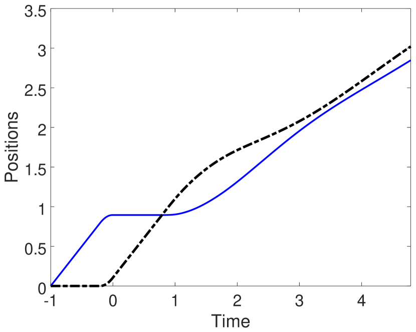
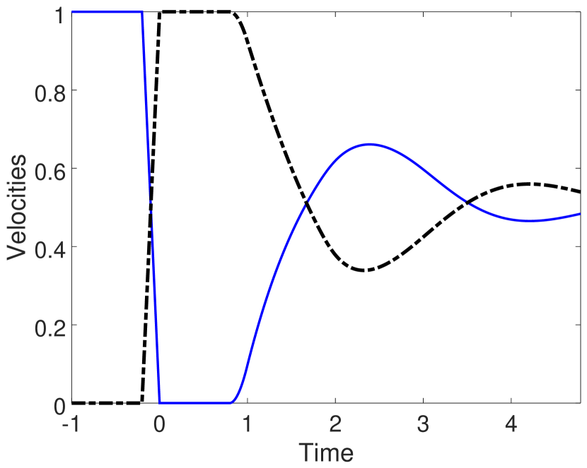
Figure 1. We simulate and plot Example 1 with $\tau=1$ and $\varepsilon=0.2$.

4.3. Example 2

Suppose that $\tau=1$, $\psi(x)=1/\sqrt{1+x^{2}}$ and

$$\left\{\begin{aligned} x^{(a)}(s)&=1+(1+s)^{2}&\text{ if }s\in[-1,0],\\ v^{(a)}(s)&=2(1+s)&\text{ if }s\in[-1,0],\\ x^{(b)}(s)&=(1+s)^{2}&\text{ if }s\in[-1,0],\\ v^{(b)}(s)&=2(1+s)&\text{ if }s\in[-1,0].\end{aligned}\right.$$ (4.8)

Note that $d_{V}(s)=0$ for all $s\in[-1,0]$ and yet we claim that

$$\max_{s\in[0,\tau]}d_{V}(s)>\frac{I_{0}}{10}.$$ (4.9)

We now prove this claim. Using the second inequality of (3.6) in the proof of Lemma 3.2 for $\mathbf{v}=1$, for each $t\in[0,1]$, we get

$$v^{(a)}(t)\geq e^{-t}v^{(a)}(0)+(1-e^{-t})\min_{c\in A}\min_{s\in[-\tau,0]}v^{(c)}(s)=2e^{-t}.$$

Then

$$v^{(a)}(t)\geq 2e^{-t}\geq 2e^{-1/2}\geq 2t$$ (4.10)

if $t\in[0,1/2]$ and the same holds for $v^{(b)}$. Therefore

$$x^{(a)}(t)-t^{2}\geq 2+\int_{0}^{t}2s\,ds-t^{2}=2$$

and we get

$$\frac{d}{dt}v^{(a)}(t) =\frac{2t-v^{(a)}(t)}{\sqrt{1+(t^{2}-x^{(a)}(t))^{2}}}\geq\sqrt{2}\frac{2t-v^{(a)}(t)}{1+x^{(a)}(t)-t^{2}}$$

where, as in (4.6), we are using that

$$\sqrt{2(1+X^{2})}\geq(1+|X|).$$

Now since

$$\frac{d}{dt}(1+x^{(a)}(t)-t^{2})=v^{(a)}(t)-2t$$

we get

$$v^{(a)}(t) \geq v^{(a)}(0)+\int_{0}^{t}(-\sqrt{2})\frac{v^{(a)}(s)-2s}{1+x^{(a)}(s)-s^{2}}\,ds$$

$$=2-\sqrt{2}\left(\ln\left(1+x^{(a)}(s)-s^{2}\right)\Big{|}_{0}^{t}\right)$$

$$=2-\sqrt{2}\ln\left(\frac{1+x^{(a)}(t)-t^{2}}{3}\right)$$

$$=2-\sqrt{2}\ln\left(\frac{1+2+\int_{0}^{t}v^{(a)}(s)\,ds-t^{2}}{3}\right)$$

$$=2-\sqrt{2}\ln\left(1+\frac{\int_{0}^{t}2\,ds-t^{2}}{3}\right)$$

$$=2-\sqrt{2}\ln\left(1+\frac{2t-t^{2}}{3}\right)$$

$$\geq 2-\sqrt{2}\ln\left(\frac{15}{4}\right)$$

for $t\in[0,1/2].$

Additionally, applying (4.3) to $v^{(b)}$ we have

$$x^{(b)}(t)-1-t^{2}\geq x^{(b)}(0)+\int_{0}^{t}v^{(b)}(s)\,ds-1-t^{2}\geq\int_{0}^{t}2s\,ds-t^{2}=0$$

and then

$$\frac{d}{dt}v^{(b)}(t) =\frac{2t-v^{(b)}(t)}{\sqrt{1+(1+t^{2}-x^{(b)}(t))^{2}}}\leq\frac{2t-v^{(b)}(t)}{1+x^{(b)}(t)-1-t^{2}}$$

because $2t-v^{(b)}(t)\leq 0$ and $\sqrt{1+X^{2}}\leq 1+|X|.$ Similarly to the case $v^{(a)}$, we get

$$v^{(b)}(t) \leq v^{(a)}(0)+\int_{0}^{t}(-1)\frac{v^{(b)}(s)-2s}{x^{(b)}(s)-s^{2}}\,ds$$

$$=2-\ln\left(x^{(b)}(t)-t^{2}\right)$$

$$\leq 2-\ln\left(1+\int_{0}^{t}v^{(b)}(s)\,ds-t^{2}\right).$$

Now assume

$$v^{(b)}(t_{0})=\min_{s\in[0,1/2]}v^{(b)}(s)$$

with $t_{0}\in[0,1/2]$. We claim that $v^{(b)}(t_{0})\leq\alpha:=1.58$. We proceed by contradiction and suppose

$$v^{(b)}(t)>\alpha$$

for each $t\in[0,1/2]$. Then

$$v^{(b)}(1/2) \leq 2-\ln\left(1+\int_{0}^{1/2}\alpha\,ds-\frac{1}{4}\right)$$

$$=2-\ln\left(1+\frac{\alpha}{2}-\frac{1}{4}\right)$$

$$<\alpha$$

and we obtain a contradiction. Finally

$$d_{V}(t_{0}) =v^{(a)}(t_{0})-v^{(b)}(t_{0})\geq 2-\sqrt{2}\ln\left(\frac{15}{4}\right)-\alpha>\frac{1}{10},$$

and we get inequality (4.9).

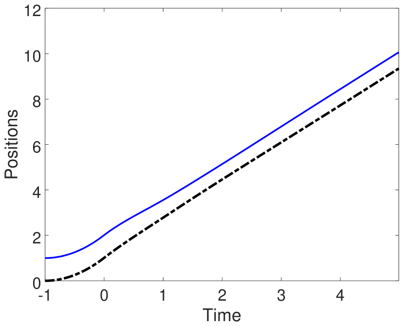
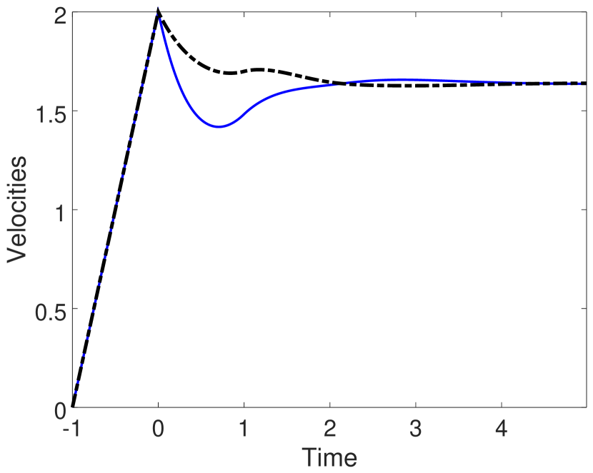
Figure 2. We simulate and plot Example 2

References

- [1] Young-Pil Choi and Jan Haskovec. Cucker-smale model with normalized communication weights and time delay. arXiv preprint arXiv:1608.06747, 2016.
- [2] Young-Pil Choi and Zhuchun Li. Emergent behavior of cucker–smale flocking particles with heterogeneous time delays. Applied Mathematics Letters, 86:49–56, 2018.
- [3] Yao-Li Chuang, Yuan R Huang, Maria R D’Orsogna, and Andrea L Bertozzi. Multi-vehicle flocking: scalability of cooperative control algorithms using pairwise potentials. In Proceedings 2007 IEEE international conference on robotics and automation, pages 2292–2299. IEEE, 2007.
- [4] Felipe Cucker and Steve Smale. Emergent behavior in flocks. IEEE Transactions on automatic control, 52(5):852–862, 2007.
- [5] Radek Erban, Jan Haskovec, and Yongzheng Sun. A cucker–smale model with noise and delay. SIAM Journal on Applied Mathematics, 76(4):1535–1557, 2016.
- [6] Seung-Yeal Ha, Jian-Guo Liu, et al. A simple proof of the cucker-smale flocking dynamics and mean-field limit. Communications in Mathematical Sciences, 7(2):297–325, 2009.
- [7] Jack K Hale. Theory of functional differential equations, volume 3 of. Applied Mathematical Sciences, 1977.
- [8] Cristina Pignotti and Emmanuel Trélat. Convergence to consensus of the general finite-dimensional cucker-smale model with time-varying delays. arXiv preprint arXiv:1707.05020, 2017.
- [9] Hal L Smith. An introduction to delay differential equations with applications to the life sciences, volume 57. Springer New York, 2011.
- [10] David JT Sumpter. Collective animal behavior. Princeton University Press, 2010.
- [11] Tamás Vicsek, András Czirók, Eshel Ben-Jacob, Inon Cohen, and Ofer Shochet. Novel type of phase transition in a system of self-driven particles. Physical review letters, 75(6):1226, 1995.