Generalized Passarino-Veltman reduction for relativistic quantum field theories at finite temperature and finite density

Abstract

The conventional Passarino-Veltman reduction (CPVR) is a systematic procedure based on the Lorentz symmetry, which can efficiently reduce the one-loop Feynman integrals (OLFIs) in the relativistic quantum field theories (RQFTs) at zero temperature and zero density. However, at finite temperature and finite density, the Lorentz symmetry is explicitly broken due to a rest reference frame of the many-body system in which the temperature and density are measured, rendering the CPVR not applicable any more to reduce OLFIs therein. In this paper, we report a generalized Passarino-Veltman reduction (GPVR), which can simplify the OLFIs in the RQFTs at finite temperature and finite density. The GPVR can analyze the OLFIs in a wide range of physical systems described by the RQFTs at finite temperature and finite density, such as quark-gluon plasma in nuclear physics.

1 Introduction

One-loop Feynman diagrams (OLFDs) play an extremely important role in calculating the transition amplitudes and correlation functions of many subfields of physics, including particle physics, nuclear physics and condensed matter physics Weinberg ; Gale ; Fetter ; Abrikosov ; Mahan . The one-by-one evaluation of OLFDs is often a time-consuming and error-prone process, therefore a very significant problem is how to most efficiently perform the OLFD calculations. Based on the Lorentz symmetry, the conventional Passarino-Veltman reduction (CPVR) CPVRS provides a powerful framework for simplifying the OLFDs Ellis ; Denner2006 . With the help of CPVR, a huge number of OLFDs can be automatically assembled from a small number of generic scalar integrals CPVRS ; Ellis ; Denner2006 . Owing to this advantage, the CPVR triggered many variants Denner2006 ; Ezawa1992 ; Tarasov1996 ; Aguila2004 ; Hameren2005 ; Beanger2006 ; Ellis2006 ; Denner2003 ; Battistel2006 ; HRC2012 ; Battistel2012 ; Oldenborgh1990 and program packages Oldenborgh1990 ; FeynArts1990 ; FeynCalc1991 ; LoopTools1999 ; QCDLoop2008 ; PackageX2015 for automatic algebraic calculation, and has been widely applied in numerous processes of high energy physics.

The precondition of applying CPVR CPVRS and its variants Ellis ; Denner2006 ; Ezawa1992 ; Tarasov1996 ; Aguila2004 ; Hameren2005 ; Beanger2006 ; Ellis2006 ; Denner2003 ; Battistel2006 ; HRC2012 ; Battistel2012 ; Oldenborgh1990 is that the physical systems of interest must respect the Lorentz symmetry, which is satisfied only in relativistic quantum field theories (RQFTs) at zero temperature and zero density (chemical potential). In the RQFTs at finite temperature and finite density, the Lorentz symmetry is explicitly broken because finite temperature or finite density specifies a rest reference frame of the many-body system in which the temperature and density are measured Gale . Consequently, the CPVR is not applicable any more to reduce OLFDs in the RQFTs at finite temperature or finite density. A natural question follows that what the counterpart of CPVR is in the RQFTs at finite temperature and finite density. On the other hand, it is known that the OLFDs in the RQFTs at finite temperature and finite density are more complicated than that at zero temperature and zero density. However, there have only been sparse attempts Rehberg1996PRC ; Rehberg1996AOP ; HRC2018 aiming at generalizing the CPVR to its counterpart at finite temperature and finite density. From both the theoretical interest and application-driven consideration, a systematic generalized Passarino-Veltman reduction (GPVR) to evaluate the OLFDs in the RQFTs at finite temperature and finite density is in need.

Motivated by these, we present a generalized reduction for simplifying the OLFDs in the RQFTs at finite temperature and finite density. The framework of GPVR for OLFDs can be straightforwardly extended from up to three-point to arbitrary-point, and hence can simplify a huge amount of OLFDs in a wide range of physical systems described by the RQFTs at finite temperature and finite density, such as quark-gluon plasma in nuclear physics.

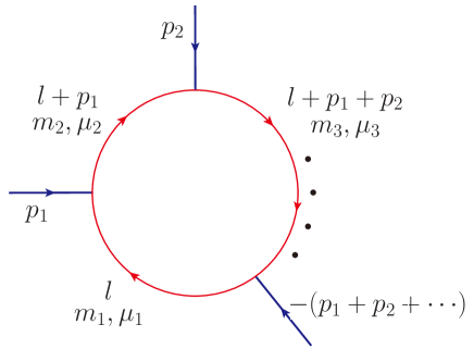
Figure 1: Generic $n$-point one-loop Feynman diagram with external momenta $p_{n}=(p_{n}^{0},\boldsymbol{p}_{n})=(p_{n}^{0},p_{n}^{i})$. The momentum of the first internal propagator is denoted by $l=(l^{0},\boldsymbol{l})=(l^{0},l^{i})$. In addition, $m_{n}$ and $\mu_{n}$ represent the mass and density of the $n$-th propagator, respectively.

2 One-loop generic scalar and tensor integrals

For the sake of simplicity and without loss of generality, we focus on the one-loop Feynman integrals (OLFIs) up to three-point in the RQFT at finite temperature and finite density, which can be decomposed into linear combinations of a series of one-loop generic scalar integrals

$$A_{0} =\int\frac{d^{D}l}{i\pi^{D/2}}\frac{1}{\mathscr{P}(l,p;m_{1},\mu_{1})},$$ (1)

$$B_{0} =\int\frac{d^{D}l}{i\pi^{D/2}}\frac{1}{\mathscr{P}(l,0;m_{1},\mu_{1})\mathscr{P}(l,p_{1};m_{2},\mu_{2})},$$ (2)

$$C_{0} =\int\frac{d^{D}l}{i\pi^{D/2}}\frac{1}{\mathscr{P}(l,0;m_{1},\mu_{1})\mathscr{P}(l,p_{1};m_{2},\mu_{2})\mathscr{P}(l,p_{1}+p_{2};m_{3},\mu_{3})},\$$ (3)

and one-loop generic tensor integrals

$$A^{\rho} =\int\frac{d^{D}l}{i\pi^{D/2}}\frac{l^{\rho}}{\mathscr{P}(l,p;m_{1},\mu_{1})},$$ (4)

$$B^{\rho};B^{\rho\sigma} =\int\frac{d^{D}l}{i\pi^{D/2}}\frac{l^{\rho};l^{\rho}l^{\sigma}}{\mathscr{P}(l,0;m_{1},\mu_{1})\mathscr{P}(l,p_{1};m_{2},\mu_{2})},$$ (5)

$$C^{\rho};C^{\rho\sigma};C^{\rho\sigma\tau} =\int\frac{d^{D}l}{i\pi^{D/2}}\frac{l^{\rho};l^{\rho}l^{\sigma};l^{\rho}l^{\sigma}l^{\tau}}{\mathscr{P}(l,0;m_{1},\mu_{1})\mathscr{P}(l,p_{1};m_{2},\mu_{2})\mathscr{P}(l,p_{1}+p_{2};m_{3},\mu_{3})},$$ (6)

where

$$\mathscr{P}(l,p;m_{n},\mu_{n}) =(l^{0}+p^{0}+\mu_{n})^{2}-\left[(\boldsymbol{l}+\boldsymbol{p})^{2}+m_{n}^{2}\right],$$ (7)

and the arguments of $\{A_{0};A^{\rho}\}$, $\{B_{0};B^{\rho};B^{\rho\sigma}\}$, and $\{C_{0};C^{\rho};C^{\rho\sigma};C^{\rho\sigma\tau}\}$ are $(p;m_{1},\mu_{1})$, $(p_{1};m_{1},\mu_{1};m_{2},\mu_{2})$, and $(p_{1},p_{2};m_{1},\mu_{1};m_{2},\mu_{2};m_{3},\mu_{3})$, respectively.

In these definitions (see Figure 1), $l=(l^{0},\boldsymbol{l})=(l^{0},l^{i})$ is the momentum of the first internal propagator, $p_{n}=(p_{n}^{0},\boldsymbol{p}_{n})=(p_{n}^{0},p_{n}^{i})$ are the external momenta, $m_{n}$ and $\mu_{n}$ denote the mass and density of the $n$-th internal propagators, respectively. In the Matsubara formalism Matsubara , the temperature are encoded into the time-component of internal momentum. Throughout this paper, we work in natural units where $\hbar=c=k_{B}=1$ and use the Greek (Roman) letters to denote the spacetime (spatial) components.

In the limit of zero temperature and zero density, these generic OLFIs restore the counterpart in the CPVR. However, at finite temperature and finite density, as a consequence of explicit breaking of the Lorentz symmetry, the largest continuous spacetime symmetry in $D$ dimension is the $\mathrm{SO}(D-1)$ spatial rotation symmetry, instead of the $\mathrm{SO}(1,D-1)$ (proper normal) Lorentz symmetry. The breaking of Lorentz symmetry leads to two crucial consequences regarding incompleteness in both tensor structures and elementary OLFIs in the RQFTs at finite temperature and density. Firstly, the Lorentz-covariant tensor structures are no longer complete to expand these generic tensor integrals which are not Lorentz-covariant. Secondly, the generic scalar integrals $A_{0}(p;m_{1},\mu_{1})$, $B_{0}(p_{1};m_{1},\mu_{1};m_{2},\mu_{2})$, and $C_{0}(p_{1},p_{2};m_{1},\mu_{1};m_{2},\mu_{2};m_{3},\mu_{3})$ are incomplete to expand all the generic one-loop tensor integrals due to the breaking of Lorentz symmetry.

The first incompleteness can be complemented by introducing an extra $D$-dimensional constant vector $u^{\rho}=(1;0,\cdots,0)$. This constant vector plays a central role in accounting for the absence of Lorentz covariance due to the presence of a rest reference frame at finite temperature and finite density Gale . Interestingly, this auxiliary vector was also introduced in developing FeynOnium for automatic calculations in non-relativistic effective field theories Shtabovenko . Treating the spacetime components of generic tensor integrals on the same footing CPVRS ; Ellis ; Denner2006 and adding the effect of Lorentz-symmetry-breaking in terms of the constant vector, the generic tensor integrals can be decomposed as that in the following section. For the second incompleteness, several elementary bubble tensor integrals $B^{0};B^{00}(p_{1};m_{1},\mu_{1};m_{2},\mu_{2})$ and elementary triangle tensor integrals $C^{0};C^{00};C^{000}(p_{1},p_{2};m_{1},\mu_{1};m_{2},\mu_{2};m_{3},\mu_{3})$ must be introduced to form a complete set of elementary integrals. These two observations motivate us to go beyond the applicability of previous works CPVRS ; Rehberg1996PRC ; Rehberg1996AOP ; HRC2018 and to develop a GPVR partially by combining the triumphs of them.

3 Reduction of generic tensor integrals

The essential procedure of CPVR is to decompose the generic tensor integrals into the corresponding generic scalar integrals. The similar story holds for the GPVR, but the substantial difference is that the generic tensor integrals must be decomposed into the corresponding generic scalar integrals and purely time-component of generic tensor integrals. In the following, we present the detailed reduction of generic tensor integrals, respectively.

3.1 Reduction of generic tadpole tensor integral $A^{\rho}(p;m_{1},\mu_{1})$

In the one-point OLFI, the time-component and spatial-component of generic tadpole tensor integral $A^{\rho}(p;m_{1},\mu_{1})$ read

$$A^{0}(p;m_{1},\mu_{1}) =\int\frac{d^{D}l}{i\pi^{D/2}}\frac{(l^{0}+p^{0}+\mu_{1})-(p^{0}+\mu_{1})}{\mathscr{P}(l,p;m_{1},\mu_{1})},$$ (8)

$$A^{i}(p;m_{1},\mu_{1}) \equiv\int\frac{d^{D}l}{i\pi^{D/2}}\frac{(l^{i}+p^{i})-p^{i}}{\mathscr{P}(l,p;m_{1},\mu_{1})}.$$ (9)

After taking the asymmetry of integrands over symmetric domain of integrals into account, one has two relations

$$\int\frac{d^{D}l}{i\pi^{D/2}}\frac{(l^{0}+p^{0}+\mu_{1})}{\mathscr{P}(l,p;m_{1},\mu_{1})} =0,$$ (10)

$$\int\frac{d^{D}l}{i\pi^{D/2}}\frac{(l^{i}+p^{i})}{\mathscr{P}(l,0;m_{1},\mu_{1})} =0,$$ (11)

which lead further to

$$A^{0}(p;m_{1},\mu_{1}) =\int\frac{d^{D}l}{i\pi^{D/2}}\frac{-(p^{0}+\mu_{1})}{\mathscr{P}(l,p;m_{1},\mu_{1})}=-(\mu_{1}+p^{0})A_{0}(p;m_{1},\mu_{1}),$$ (12)

$$A^{i}(p;m_{1},\mu_{1}) =\int\frac{d^{D}l}{i\pi^{D/2}}\frac{-p^{i}}{\mathscr{P}(l,p;m_{1},\mu_{1})}=-p^{i}A_{0}(p;m_{1},\mu_{1}),$$ (13)

indicating that both $A^{0}(p;m_{1},\mu_{1})$ and $A^{i}(p;m_{1},\mu_{1})$ can be expressed by $A_{0}(p;m_{1},\mu_{1})$.

That is, the generic tadpole tensor integral $A^{\rho}(p;m_{1},\mu_{1})$ can be reduced to

$$A^{\rho}(p;m_{1},\mu_{1}) \equiv\int\frac{d^{D}l}{i\pi^{D/2}}\frac{l^{\rho}}{\mathscr{P}(l,p;m_{1},\mu_{1})}=-\left(\mu_{1}\delta^{\rho 0}+p^{\rho}\right)A_{0}(p;m_{1},\mu_{1}).$$ (14)

It is also interesting to note that the generic tadpole scalar integral

$$A_{0}(p;m_{1},\mu_{1}) \equiv\int\frac{d^{D}l}{i\pi^{D/2}}\frac{1}{\mathscr{P}(l,p;m_{1},\mu_{1})}=\int\frac{d^{D}l}{i\pi^{D/2}}\frac{1}{\mathscr{P}(l,0;m_{1},\mu_{1})}=A_{0}(0;m_{1},\mu_{1})$$ (15)

by shifting the loop momentum $l$ to $l-p_{1}$.

In short, the generic tadpole tensor integral $A^{\rho}(p;m_{1},\mu_{1})$ can be reduced to the generic tadpole scalar integral $A_{0}(p;m_{1},\mu_{1})=A_{0}(0;m_{1},\mu_{1})$.

3.2 Reduction of generic bubble tensor integral $B^{\rho}(p_{1};m_{1},\mu_{1};m_{2},\mu_{2})$

In the two-point OLFIs, the generic bubble tensor integral $B^{\rho}(p_{1};m_{1},\mu_{1};m_{2},\mu_{2})$ can be reduced as

$$B^{\rho}(p_{1};m_{1},\mu_{1};m_{2},\mu_{2}) =\int\frac{d^{D}l}{i\pi^{D/2}}\frac{l^{\rho}}{\mathscr{P}(l,0;m_{1},\mu_{1})\mathscr{P}(l,p_{1};m_{2},\mu_{2})}$$

$$=u^{\rho}\mathcal{B}_{1}+p_{1}^{\rho}\mathcal{B}_{2}$$ (16)

where the arguments $(p_{1};m_{1},\mu_{1};m_{2},\mu_{2})$ in the form factors $\mathcal{B}_{1}$ and $\mathcal{B}_{2}$ are omitted for short.

Contracting the genetic bubble tensor integral $B^{\rho}(p_{1};m_{1},\mu_{1};m_{2},\mu_{2})$ with $u_{\rho}$ and $p_{1\rho}$ gives rise to two equations,

$$\left(\begin{array}[]{cc}1&\hskip 14.22636ptp_{1}^{0}\\ \\ p_{1}^{0}&\hskip 14.22636ptp_{1}^{2}\\ \end{array}\right)\left(\begin{array}[]{c}\mathcal{B}_{1}\\ \\ \mathcal{B}_{2}\\ \end{array}\right) =\left(\begin{array}[]{c}\mathcal{F}_{1}\\ \\ \mathcal{F}_{2}\\ \end{array}\right),$$ (26)

where

$$\mathcal{F}_{1} =u_{\rho}B^{\rho}(p_{1};m_{1},\mu_{1};m_{2},\mu_{2})$$

$$=\int\frac{d^{D}l}{i\pi^{D/2}}\frac{u\cdot l}{\mathscr{P}(l,0;m_{1},\mu_{1})\mathscr{P}(l,p_{1};m_{2},\mu_{2})}$$

$$=\int\frac{d^{D}l}{i\pi^{D/2}}\frac{l^{0}}{\mathscr{P}(l,0;m_{1},\mu_{1})\mathscr{P}(l,p_{1};m_{2},\mu_{2})},$$ (27)

$$\mathcal{F}_{2} =p_{1\rho}B^{\rho}(p_{1};m_{1},\mu_{1};m_{2},\mu_{2})$$

$$=\frac{1}{2}\int\frac{d^{D}l}{i\pi^{D/2}}\frac{2p_{1}\cdot l}{\mathscr{P}(l,0;m_{1},\mu_{1})\mathscr{P}(l,p_{1};m_{2},\mu_{2})}.$$ (28)

By solving these two equations, the form factors $\mathcal{B}_{1}$ and $\mathcal{B}_{2}$ can be expressed in terms of $\mathcal{F}_{1}$ and $\mathcal{F}_{2}$. As for $\mathcal{F}_{1}$, it is straightforward that

$$\mathcal{F}_{1} =B^{0}(p_{1};m_{1},\mu_{1};m_{2},\mu_{2}).$$ (29)

As for $\mathcal{F}_{2}$, after utilizing the decomposition

$$2p_{1}\cdot l =2p_{1}^{0}l^{0}-2\boldsymbol{l}\cdot\boldsymbol{p}_{1}=2p_{1}^{0}l^{0}+\boldsymbol{l}^{2}+\boldsymbol{p}_{1}^{2}-(\boldsymbol{l}+\boldsymbol{p}_{1})^{2}$$

$$=\left\{\left(\mu_{1}^{2}-m_{1}^{2}\right)-\left[(\mu_{2}+p_{1}^{0})^{2}-m_{2}^{2}\right]+\boldsymbol{p}_{1}^{2}\right\}$$

$$\hskip 8.5359pt-2\left(\mu_{2}-\mu_{1}\right)l^{0}+\mathscr{P}(l,p_{1};m_{2},\mu_{2})-\mathscr{P}(l,0;m_{1},\mu_{1}),$$ (30)

we have

$$\mathcal{F}_{2} =\frac{\left\{\left(\mu_{1}^{2}-m_{1}^{2}\right)-\left[(\mu_{2}+p_{1}^{0})^{2}-m_{2}^{2}\right]+\boldsymbol{p}_{1}^{2}\right\}B_{0}(p_{1};m_{1},\mu_{1};m_{2},\mu_{2})}{2}$$

$$\hskip 8.5359pt-\left(\mu_{2}-\mu_{1}\right)B^{0}(p_{1};m_{1},\mu_{1};m_{2},\mu_{2})+\frac{A_{0}(0;m_{1},\mu_{1})-A_{0}(0;m_{2},\mu_{2})}{2}.$$ (31)

Briefly, the generic bubble tensor integral $B^{\rho}(p_{1};m_{1},\mu_{1};m_{2},\mu_{2})$ can be decomposed as linear combinations of tensor structures $u^{\rho}$ and $p_{1}^{\rho}$ with the form factors $\mathcal{B}_{1}$ and $\mathcal{B}_{2}$ being expressed by the generic tadpole scalar integral $A_{0}(p_{1};m_{1},\mu_{1})$, generic bubble scalar integral $B_{0}(p_{1};m_{1},\mu_{1};m_{2},\mu_{2})$, and a time-component of generic bubble tensor integral $B^{0}(p_{1};m_{1},\mu_{1};m_{2},\mu_{2})$.

3.3 Reduction of generic bubble tensor integral $B^{\rho\sigma}(p_{1};m_{1},\mu_{1};m_{2},\mu_{2})$

In the two-point OLFIs, the generic bubble tensor integral $B^{\rho}(p_{1};m_{1},\mu_{1};m_{2},\mu_{2})$ can be reduced as

$$B^{\rho\sigma}(p_{1};m_{1},\mu_{1};m_{2},\mu_{2}) =\int\frac{d^{D}l}{i\pi^{D/2}}\frac{l^{\rho}l^{\sigma}}{\mathscr{P}(l,0;m_{1},\mu_{1})\mathscr{P}(l,p_{1};m_{2},\mu_{2})}$$

$$=g^{\rho\sigma}\mathcal{B}_{00}+u^{\rho}u^{\sigma}\mathcal{B}_{11}+\left(u^{\rho}p_{1}^{\sigma}+p_{1}^{\rho}u^{\sigma}\right)\mathcal{B}_{12}+p_{1}^{\rho}p_{1}^{\sigma}\mathcal{B}_{22},$$ (32)

where $\mathcal{B}_{ab}=\mathcal{B}_{ba}$ and the arguments $(p_{1};m_{1},\mu_{1};m_{2},\mu_{2})$ in the form factors $\mathcal{B}_{1}$ and $\mathcal{B}_{2}$ are omitted for short.

Contracting the genetic bubble tensor integral $B^{\rho\sigma}(p_{1};m_{1},\mu_{1};m_{2},\mu_{2})$ with $g_{\rho\sigma}$, $u_{\rho}u_{\sigma}$, $u_{\rho}p_{1\sigma}$, and $p_{1\rho}p_{1\sigma}$ gives rise to four equations,

$$\left(\begin{array}[]{cccc}D&\hskip 14.22636pt1&\hskip 14.22636pt2p_{1}^{0}&\hskip 14.22636ptp_{1}^{2}\\ \\ 1&\hskip 14.22636pt1&\hskip 14.22636pt2p_{1}^{0}&\hskip 14.22636pt(p_{1}^{0})^{2}\\ \\ p_{1}^{0}&\hskip 14.22636ptp_{1}^{0}&\hskip 14.22636pt(p_{1}^{0})^{2}+p_{1}^{2}&\hskip 14.22636ptp_{1}^{0}p_{1}^{2}\\ \\ p_{1}^{2}&\hskip 14.22636pt(p_{1}^{0})^{2}&\hskip 14.22636pt2p_{1}^{0}p_{1}^{2}&\hskip 14.22636pt(p_{1}^{2})^{2}\\ \end{array}\right)\left(\begin{array}[]{c}\mathcal{B}_{00}\\ \\ \mathcal{B}_{11}\\ \\ \mathcal{B}_{12}\\ \\ \mathcal{B}_{22}\\ \end{array}\right)=\left(\begin{array}[]{c}\mathcal{F}_{00}\\ \\ \mathcal{F}_{11}\\ \\ \mathcal{F}_{12}\\ \\ \mathcal{F}_{22}\\ \end{array}\right),$$ (54)

where

$$\mathcal{F}_{00} =g_{\rho\sigma}B^{\rho\sigma}(p_{1};m_{1},\mu_{1};m_{2},\mu_{2})$$

$$=\int\frac{d^{D}l}{i\pi^{D/2}}\frac{l^{2}}{\mathscr{P}(l,0;m_{1},\mu_{1})\mathscr{P}(l,p_{1};m_{2},\mu_{2})},$$ (55)

$$\mathcal{F}_{11} =u_{\rho}u_{\sigma}B^{\rho\sigma}(p_{1};m_{1},\mu_{1};m_{2},\mu_{2})$$

$$=\int\frac{d^{D}l}{i\pi^{D/2}}\frac{(u\cdot l)(u\cdot l)}{\mathscr{P}(l,0;m_{1},\mu_{1})\mathscr{P}(l,p_{1};m_{2},\mu_{2})}$$

$$=\int\frac{d^{D}l}{i\pi^{D/2}}\frac{l^{0}l^{0}}{\mathscr{P}(l,0;m_{1},\mu_{1})\mathscr{P}(l,p_{1};m_{2},\mu_{2})},$$ (56)

$$\mathcal{F}_{12} =u_{\rho}p_{1\sigma}B^{\rho\sigma}(p_{1};m_{1},\mu_{1};m_{2},\mu_{2})$$

$$=\int\frac{d^{D}l}{i\pi^{D/2}}\frac{(u\cdot l)(p_{1}\cdot l)}{\mathscr{P}(l,0;m_{1},\mu_{1})\mathscr{P}(l,p_{1};m_{2},\mu_{2})}$$

$$=\int\frac{d^{D}l}{i\pi^{D/2}}\frac{l^{0}(p_{1}\cdot l)}{\mathscr{P}(l,0;m_{1},\mu_{1})\mathscr{P}(l,p_{1};m_{2},\mu_{2})},$$ (57)

$$\mathcal{F}_{22} =p_{1\rho}p_{1\sigma}B^{\rho\sigma}(p_{1};m_{1},\mu_{1};m_{2},\mu_{2})$$

$$=\int\frac{d^{D}l}{i\pi^{D/2}}\frac{(p_{1}\cdot l)^{2}}{\mathscr{P}(l,0;m_{1},\mu_{1})\mathscr{P}(l,p_{1};m_{2},\mu_{2})}.$$ (58)

By solving these four equations, the form factors $\mathcal{B}_{00}$, $\mathcal{B}_{11}$, $\mathcal{B}_{12}$, and $\mathcal{B}_{22}$ can be expressed in terms of $\mathcal{F}_{00}$, $\mathcal{F}_{11}$, $\mathcal{F}_{12}$, and $\mathcal{F}_{22}$. As for $\mathcal{F}_{00}$, after utilizing the decomposition

$$l^{2} =(l^{0})^{2}-\boldsymbol{l}^{2}=-\left(\mu_{1}^{2}-m_{1}^{2}\right)-2\mu_{1}l^{0}+\mathscr{P}(l,0;m_{1},\mu_{1}),$$ (59)

we have

$$\mathcal{F}_{00}= -\left(\mu_{1}^{2}-m_{1}^{2}\right)B_{0}(p_{1};m_{1},\mu_{1};m_{2},\mu_{2})$$

$$-2\mu_{1}B^{0}(p_{1};m_{1},\mu_{1};m_{2},\mu_{2})+A_{0}(0;m_{2},\mu_{2}).$$ (60)

It is straightforward to get

$$\mathcal{F}_{11} =B^{00}(p_{1};m_{1},\mu_{1};m_{2},\mu_{2}).$$ (61)

As for $\mathcal{F}_{12}$, after utilizing the decomposition

$$2l^{0}(p_{1}\cdot l) =\left\{\left(\mu_{1}^{2}-m_{1}^{2}\right)-\left[(\mu_{2}+p_{1}^{0})^{2}-m_{2}^{2}\right]+\boldsymbol{p}_{1}^{2}\right\}l^{0}-2\left(\mu_{2}-\mu_{1}\right)l^{0}l^{0}$$

$$\hskip 8.5359pt+\mathscr{P}(l,p_{1};m_{2},\mu_{2})l^{0}-\mathscr{P}(l,0;m_{1},\mu_{1})l^{0},$$ (62)

we have

$$\mathcal{F}_{12} =\frac{\left\{\left(\mu_{1}^{2}-m_{1}^{2}\right)-\left[(\mu_{2}+p_{1}^{0})^{2}-m_{2}^{2}\right]+\boldsymbol{p}_{1}^{2}\right\}}{2}B^{0}(p_{1};m_{1},\mu_{1};m_{2},\mu_{2})$$

$$\hskip 8.5359pt-\left(\mu_{2}-\mu_{1}\right)B^{00}(p_{1};m_{1},\mu_{1};m_{2},\mu_{2})+\frac{A^{0}(0;m_{1},\mu_{1})-A^{0}(p_{1};m_{2},\mu_{2})}{2}.$$ (63)

As for $\mathcal{F}_{22}$, after utilizing the decomposition

$$(2p_{1}\cdot l)^{2} =\left[\mathscr{P}(l,p_{1};m_{2},\mu_{2})-\mathscr{P}(l,0;m_{1},\mu_{1})\right]^{2}$$

$$\hskip 8.5359pt+\left\{\left(\mu_{1}^{2}-m_{1}^{2}\right)-\left[(\mu_{2}+p_{1}^{0})^{2}-m_{2}^{2}\right]+\boldsymbol{p}_{1}^{2}\right\}^{2}-4\left(\mu_{2}-\mu_{1}\right)^{2}l^{0}l^{0}$$

$$\hskip 8.5359pt-4\left(\mu_{2}-\mu_{1}\right)\left[\mathscr{P}(l,p_{1};m_{2},\mu_{2})-\mathscr{P}(l,0;m_{1},\mu_{1})\right]l^{0}$$

$$\hskip 8.5359pt+2\left\{\left(\mu_{1}^{2}-m_{1}^{2}\right)-\left[(\mu_{2}+p_{1}^{0})^{2}-m_{2}^{2}\right]+\boldsymbol{p}_{1}^{2}\right\}\left[\mathscr{P}(l,p_{1};m_{2},\mu_{2})-\mathscr{P}(l,0;m_{1},\mu_{1})\right]$$

$$\hskip 8.5359pt-4\left(\mu_{2}-\mu_{1}\right)\left\{\left(\mu_{1}^{2}-m_{1}^{2}\right)-\left[(\mu_{2}+p_{1}^{0})^{2}-m_{2}^{2}\right]+\boldsymbol{p}_{1}^{2}\right\}l^{0},$$ (64)

and performing the integrations

$$\int\frac{d^{D}l}{i\pi^{D/2}}\left[\frac{\mathscr{P}(l,p_{1};m_{2},\mu_{2})}{\mathscr{P}(l,0;m_{1},\mu_{1})}-1\right]$$

$$=\int\frac{d^{D}l}{i\pi^{D/2}}\left[\frac{2\left(\mu_{2}+p_{1}^{0}-\mu_{1}\right)(l^{0}+\mu_{1})+(\mu_{2}+p_{1}^{0}-\mu_{1})^{2}+\left(\boldsymbol{p}_{1}^{2}+m_{1}^{2}-m_{2}^{2}\right)-2\boldsymbol{l}\cdot\boldsymbol{p}_{1}}{\mathscr{P}(l,0;m_{1},\mu_{1})}\right]$$

$$=2\left(\mu_{2}+p_{1}^{0}-\mu_{1}\right)A^{0}(0;m_{1},\mu_{1})$$

$$\hskip 8.5359pt-\left\{\left(\mu_{1}^{2}-m_{1}^{2}\right)-\left[(\mu_{2}+p_{1}^{0})^{2}-m_{2}^{2}\right]+\boldsymbol{p}_{1}^{2}\right\}A_{0}(0;m_{1},\mu_{1}),$$ (65)

$$\int\frac{d^{D}l}{i\pi^{D/2}}\left[\frac{\mathscr{P}(l,0;m_{1},\mu_{1})}{\mathscr{P}(l,p_{1};m_{2},\mu_{2})}-1\right]$$

$$=\int\frac{d^{D}l}{i\pi^{D/2}}\left[\frac{-2\left(\mu_{2}+p_{1}^{0}-\mu_{1}\right)(l^{0}+\mu_{2}+p_{1}^{0})+(\mu_{2}+p_{1}^{0}-\mu_{1})^{2}+\left(\boldsymbol{p}_{1}^{2}-m_{1}^{2}+m_{2}^{2}\right)+2\boldsymbol{l}\cdot\boldsymbol{p}_{1}}{\mathscr{P}(l,p_{1};m_{2},\mu_{2})}\right]$$

$$=-2\left(\mu_{2}+p_{1}^{0}-\mu_{1}\right)A^{0}(p_{1};m_{2},\mu_{2})$$

$$\hskip 8.5359pt+\left\{\left(\mu_{1}^{2}-m_{1}^{2}\right)-\left[(\mu_{2}+p_{1}^{0})^{2}-m_{2}^{2}\right]+\boldsymbol{p}_{1}^{2}\right\}A_{0}(p_{1};m_{2},\mu_{2}).$$ (66)

we have

$$\mathcal{F}_{22} =\frac{\left\{\left(\mu_{1}^{2}-m_{1}^{2}\right)-\left[(\mu_{2}+p_{1}^{0})^{2}-m_{2}^{2}\right]+\boldsymbol{p}_{1}^{2}\right\}^{2}B_{0}(p_{1};m_{1},\mu_{1};m_{2},\mu_{2})}{4}$$

$$\hskip 8.5359pt+\left(\mu_{2}-\mu_{1}\right)^{2}B^{00}(p_{1};m_{1},\mu_{1};m_{2},\mu_{2})$$

$$\hskip 8.5359pt-\left(\mu_{2}-\mu_{1}\right)\left\{\left(\mu_{1}^{2}-m_{1}^{2}\right)-\left[(\mu_{2}+p_{1}^{0})^{2}-m_{2}^{2}\right]+\boldsymbol{p}_{1}^{2}\right\}B^{0}(p_{1};m_{1},\mu_{1};m_{2},\mu_{2})$$

$$\hskip 8.5359pt+\left[2\left(\mu_{2}+p_{1}^{0}-\mu_{1}\right)-\left(\mu_{2}-\mu_{1}\right)\right]\left[A^{0}(0;m_{1},\mu_{1})-A^{0}(p_{1};m_{2},\mu_{2})\right]$$

$$\hskip 8.5359pt-\frac{\left\{\left(\mu_{1}^{2}-m_{1}^{2}\right)-\left[(\mu_{2}+p_{1}^{0})^{2}-m_{2}^{2}\right]+\boldsymbol{p}_{1}^{2}\right\}}{2}\left[A_{0}(0;m_{1},\mu_{1})-A_{0}(p_{1};m_{2},\mu_{2})\right].$$ (67)

Consequently, the generic bubble tensor integral $B^{\rho\sigma}(p_{1};m_{1},\mu_{1};m_{2},\mu_{2})$ can be decomposed as linear combinations of tensor structures $g^{\rho\sigma}$, $u^{\rho}u^{\sigma}$, $\left(u^{\rho}p_{1}^{\sigma}+p_{1}^{\rho}u^{\sigma}\right)$ and $+p_{1}^{\rho}p_{1}^{\sigma}$ with the form factors $\mathcal{B}_{00}$, $\mathcal{B}_{11}$, $\mathcal{B}_{12}$, and $\mathcal{B}_{22}$ being expressed by the generic tadpole scalar integral $A_{0}(p_{1};m_{1},\mu_{1})$, generic bubble scalar integral $B_{0}(p_{1};m_{1},\mu_{1};m_{2},\mu_{2})$, and two time-components of generic bubble tensor integrals $B^{0}(p_{1};m_{1},\mu_{1};m_{2},\mu_{2})$ and $B^{00}(p_{1};m_{1},\mu_{1};m_{2},\mu_{2})$.

3.4 Reduction for generic triangle tensor integral $C^{\rho}(p_{1},p_{2};m_{1},\mu_{1};m_{2},\mu_{2};m_{3},\mu_{3})$

In the three-point OLFIs, the generic triangle tensor integral $C^{\rho}(p_{1},p_{2};m_{1},\mu_{1};m_{2},\mu_{2};m_{3},\mu_{3})$ can be reduced as

$$C^{\rho}(p_{1},p_{2};m_{1},\mu_{1};m_{2},\mu_{2};m_{3},\mu_{3})$$

$$\hskip 56.9055pt=\int\frac{d^{D}l}{i\pi^{D/2}}\frac{l^{\rho}}{\mathscr{P}(l,0;m_{1},\mu_{1})\mathscr{P}(l,p_{1};m_{2},\mu_{2})\mathscr{P}(l,p_{1}+p_{2};m_{3},\mu_{3})}$$

$$\hskip 56.9055pt=u^{\rho}\mathcal{C}_{1}+p_{1}^{\rho}\mathcal{C}_{2}+p_{2}^{\rho}\mathcal{C}_{3},$$ (68)

where the arguments $(p_{1},p_{2};m_{1},\mu_{1};m_{2},\mu_{2};m_{3},\mu_{3})$ in $\mathcal{C}_{1}$, $\mathcal{C}_{2}$, and $\mathcal{C}_{3}$ are omitted for short.

Contracting the genetic bubble tensor integral $C^{\rho}(p_{1},p_{2};m_{1},\mu_{1};m_{2},\mu_{2};m_{3},\mu_{3})$ with $u_{\rho}$, $p_{1\rho}$, and $p_{2\rho}$ gives rise to three equations,

$$\left(\begin{array}[]{ccc}1&\hskip 28.45274ptp_{1}^{0}&\hskip 28.45274ptp_{2}^{0}\\ \\ p_{1}^{0}&\hskip 28.45274ptp_{1}^{2}&\hskip 28.45274ptp_{1}\cdot p_{2}\\ \\ p_{2}^{0}&\hskip 28.45274ptp_{1}\cdot p_{2}&\hskip 28.45274ptp_{2}^{2}\\ \end{array}\right)\left(\begin{array}[]{c}\mathcal{C}_{1}\\ \\ \mathcal{C}_{2}\\ \\ \mathcal{C}_{3}\\ \end{array}\right)=\left(\begin{array}[]{c}\mathcal{G}_{1}\\ \\ \mathcal{G}_{2}\\ \\ \mathcal{G}_{3}\\ \end{array}\right),$$ (84)

where

$$\mathcal{G}_{1} =u_{\rho}C^{\rho}(p_{1},p_{2};m_{1},\mu_{1};m_{2},\mu_{2};m_{3},\mu_{3})$$

$$=\int\frac{d^{D}l}{i\pi^{D/2}}\frac{u\cdot l}{\mathscr{P}(l,0;m_{1},\mu_{1})\mathscr{P}(l,p_{1};m_{2},\mu_{2})\mathscr{P}(l,p_{1}+p_{2};m_{3},\mu_{3})}$$

$$=\int\frac{d^{D}l}{i\pi^{D/2}}\frac{l^{0}}{\mathscr{P}(l,0;m_{1},\mu_{1})\mathscr{P}(l,p_{1};m_{2},\mu_{2})\mathscr{P}(l,p_{1}+p_{2};m_{3},\mu_{3})},$$ (85)

$$\mathcal{G}_{2} =p_{1\rho}C^{\rho}(p_{1},p_{2};m_{1},\mu_{1};m_{2},\mu_{2};m_{3},\mu_{3})$$

$$=\int\frac{d^{D}l}{i\pi^{D/2}}\frac{p_{1}\cdot l}{\mathscr{P}(l,0;m_{1},\mu_{1})\mathscr{P}(l,p_{1};m_{2},\mu_{2})\mathscr{P}(l,p_{1}+p_{2};m_{3},\mu_{3})},$$ (86)

$$\mathcal{G}_{3} =p_{2\rho}C^{\rho}(p_{1},p_{2};m_{1},\mu_{1};m_{2},\mu_{2};m_{3},\mu_{3})$$

$$=\int\frac{d^{D}l}{i\pi^{D/2}}\frac{p_{2}\cdot l}{\mathscr{P}(l,0;m_{1},\mu_{1})\mathscr{P}(l,p_{1};m_{2},\mu_{2})\mathscr{P}(l,p_{1}+p_{2};m_{3},\mu_{3})}.$$ (87)

By solving these three equations, the form factors $\mathcal{C}_{1}$, $\mathcal{C}_{2}$, and $\mathcal{C}_{3}$ can be expressed in terms of $\mathcal{G}_{1}$, $\mathcal{G}_{2}$, and $\mathcal{G}_{3}$. As for $\mathcal{G}_{1}$, after utilizing the decomposition

$$\mathcal{G}_{1} =C^{0}(p_{1},p_{2};m_{1},\mu_{1};m_{2},\mu_{2};m_{3},\mu_{3}).$$ (88)

As for $\mathcal{G}_{2}$, after utilizing the decomposition

$$2p_{1}\cdot l =2p_{1}^{0}l^{0}-2\boldsymbol{l}\cdot\boldsymbol{p}_{1}=2p_{1}^{0}l^{0}+\boldsymbol{l}^{2}+\boldsymbol{p}_{1}^{2}-(\boldsymbol{l}+\boldsymbol{p}_{1})^{2}$$

$$=\left[\left(\mu_{1}^{2}-m_{1}^{2}\right)-\left((\mu_{2}+p_{1}^{0})^{2}-m_{2}^{2}\right)+\boldsymbol{p}_{1}^{2}\right]$$

$$\hskip 8.5359pt-2\left(\mu_{2}-\mu_{1}\right)l^{0}+\mathscr{P}(l,p_{1};m_{2},\mu_{2})-\mathscr{P}(l,0;m_{1},\mu_{1}),$$ (89)

we have

$$\mathcal{G}_{2} =\frac{\left[\left(\mu_{1}^{2}-m_{1}^{2}\right)-\left((\mu_{2}+p_{1}^{0})^{2}-m_{2}^{2}\right)+\boldsymbol{p}_{1}^{2}\right]}{2}C_{0}(p_{1},p_{2};m_{1},\mu_{1};m_{2},\mu_{2};m_{3},\mu_{3})$$

$$\hskip 8.5359pt-\left(\mu_{2}-\mu_{1}\right)C^{0}(p_{1},p_{2};m_{1},\mu_{1};m_{2},\mu_{2};m_{3},\mu_{3})$$

$$\hskip 8.5359pt+\frac{B_{0}(p_{1}+p_{2};m_{1},\mu_{1};m_{3},\mu_{3})-B_{0}(p_{2};m_{2},\mu_{2};m_{3},\mu_{3})}{2}.$$ (90)

As for $\mathcal{G}_{3}$, after utilizing the decomposition

$$2p_{2}\cdot l =\left\{\left[(\mu_{2}+p_{1}^{0})^{2}-m_{2}^{2}-\boldsymbol{p}_{1}^{2}\right]-\left[(\mu_{3}+p_{1}^{0}+p_{2}^{0})^{2}-m_{3}^{2}-(\boldsymbol{p}_{1}+\boldsymbol{p}_{2})^{2}\right]\right\}$$

$$\hskip 8.5359pt-2\left(\mu_{3}-\mu_{2}\right)l^{0}+\mathscr{P}(l,p_{1}+p_{2};3)-\mathscr{P}(l,p_{1};2),$$ (91)

we have

$$\mathcal{G}_{3} =\frac{\left[(\mu_{2}+p_{1}^{0})^{2}-m_{2}^{2}-\boldsymbol{p}_{1}^{2}\right]-\left[(\mu_{3}+p_{1}^{0}+p_{2}^{0})^{2}-m_{3}^{2}-(\boldsymbol{p}_{1}+\boldsymbol{p}_{2})^{2}\right]}{2}$$

$$\hskip 8.5359pt\times C_{0}(p_{1},p_{2};m_{1},\mu_{1};m_{2},\mu_{2};m_{3},\mu_{3})$$

$$\hskip 8.5359pt-\left(\mu_{3}-\mu_{2}\right)C^{0}(p_{1},p_{2};m_{1},\mu_{1};m_{2},\mu_{2};m_{3},\mu_{3})$$

$$\hskip 8.5359pt+\frac{B_{0}(p_{1};m_{1},\mu_{1};m_{2},\mu_{2})-B_{0}(p_{1}+p_{2};m_{1},\mu_{1};m_{3},\mu_{3})}{2}.$$ (92)

To sum up, the generic bubble tensor integral $C^{\rho}(p_{1},p_{2};m_{1},\mu_{1};m_{2},\mu_{2};m_{3},\mu_{3})$ can be decomposed as linear combinations of tensor structures $u^{\rho}$, $p_{1}^{\rho}$, and $p_{2}^{\rho}$ with the form factors $\mathcal{C}_{1}$, $\mathcal{C}_{2}$, and $\mathcal{C}_{2}$ being expressed by the generic bubble scalar integral $B_{0}(p_{1};m_{1},\mu_{1};m_{2},\mu_{2})$, $C_{0}(p_{1},p_{2};m_{1},\mu_{1};m_{2},\mu_{2};m_{3},\mu_{3})$, and a time-component of generic triangle tensor integral $C^{0}(p_{1},p_{2};m_{1},\mu_{1};m_{2},\mu_{2};m_{3},\mu_{3})$.

3.5 Reduction for generic triangle tensor integrals $C^{\rho\sigma}(p_{1},p_{2};m_{1},\mu_{1};m_{2},\mu_{2};m_{3},\mu_{3})$ and $C^{\rho\sigma\tau}(p_{1},p_{2};m_{1},\mu_{1};m_{2},\mu_{2};m_{3},\mu_{3})$

In the three-point OLFIs, two other genetic triangle tensor integrals can be reduced in the similar way as

$$C^{\rho\sigma}(p_{1},p_{2};m_{1},\mu_{1};m_{2},\mu_{2};m_{3},\mu_{3})$$

$$\hskip 56.9055pt=\int\frac{d^{D}l}{i\pi^{D/2}}\frac{l^{\rho}l^{\sigma}}{\mathscr{P}(l,0;m_{1},\mu_{1})\mathscr{P}(l,p_{1};m_{2},\mu_{2})\mathscr{P}(l,p_{1}+p_{2};m_{3},\mu_{3})}$$

$$\hskip 56.9055pt=g^{\rho\sigma}\mathcal{C}_{00}+u^{\rho}u^{\sigma}\mathcal{C}_{11}+\left(u^{\rho}p_{1}^{\sigma}+p_{1}^{\rho}u^{\sigma}\right)\mathcal{C}_{12}+\left(u^{\rho}p_{2}^{\sigma}+p_{2}^{\rho}u^{\sigma}\right)\mathcal{C}_{13}$$

$$\hskip 65.44142pt+p_{1}^{\rho}p_{1}^{\sigma}\mathcal{C}_{22}+\left(p_{1}^{\rho}p_{2}^{\sigma}+p_{2}^{\rho}p_{1}^{\sigma}\right)\mathcal{C}_{23}+p_{2}^{\rho}p_{2}^{\sigma}\mathcal{C}_{33},$$

and

$$C^{\rho\sigma\tau}(p_{1},p_{2};m_{1},\mu_{1};m_{2},\mu_{2};m_{3},\mu_{3})$$

$$\hskip 56.9055pt=\int\frac{d^{D}l}{i\pi^{D/2}}\frac{l^{\rho}l^{\sigma}l^{\tau}}{\mathscr{P}(l,0;m_{1},\mu_{1})\mathscr{P}(l,p_{1};m_{2},\mu_{2})\mathscr{P}(l,p_{1}+p_{2};m_{3},\mu_{3})}$$

$$\hskip 56.9055pt=\left(g^{\rho\sigma}u^{\tau}+g^{\sigma\tau}u^{\rho}+g^{\tau\rho}u^{\sigma}\right)\mathcal{C}_{001}$$

$$\hskip 65.44142pt+\left(g^{\rho\sigma}p_{1}^{\tau}+g^{\sigma\tau}p_{1}^{\rho}+g^{\tau\rho}p_{1}^{\sigma}\right)\mathcal{C}_{002}$$

$$\hskip 65.44142pt+\left(g^{\rho\sigma}p_{2}^{\tau}+g^{\sigma\tau}p_{2}^{\rho}+g^{\tau\rho}p_{2}^{\sigma}\right)\mathcal{C}_{003}$$

$$\hskip 65.44142pt+u^{\rho}u^{\sigma}u^{\tau}\mathcal{C}_{111}+p_{1}^{\rho}p_{1}^{\sigma}p_{1}^{\tau}\mathcal{C}_{222}+p_{2}^{\rho}p_{2}^{\sigma}p_{2}^{\tau}\mathcal{C}_{333}$$

$$\hskip 65.44142pt+\left(u^{\rho}u^{\sigma}p_{1}^{\tau}+u^{\rho}p_{1}^{\sigma}u^{\tau}+p_{1}^{\rho}u^{\sigma}u^{\tau}\right)\mathcal{C}_{112}$$

$$\hskip 65.44142pt+\left(u^{\rho}u^{\sigma}p_{2}^{\tau}+u^{\rho}p_{2}^{\sigma}u^{\tau}+p_{2}^{\rho}u^{\sigma}u^{\tau}\right)\mathcal{C}_{113}$$

$$\hskip 65.44142pt+\left(p_{1}^{\rho}p_{1}^{\sigma}u^{\tau}+p_{1}^{\rho}u^{\sigma}p_{1}^{\tau}+u^{\rho}p_{1}^{\sigma}p_{1}^{\tau}\right)\mathcal{C}_{122}$$

$$\hskip 65.44142pt+\left(p_{2}^{\rho}p_{2}^{\sigma}u^{\tau}+p_{2}^{\rho}u^{\sigma}p_{2}^{\tau}+u^{\rho}p_{2}^{\sigma}p_{2}^{\tau}\right)\mathcal{C}_{133}$$

$$\hskip 65.44142pt+\left(p_{1}^{\rho}p_{1}^{\sigma}p_{2}^{\tau}+p_{1}^{\rho}p_{2}^{\sigma}p_{1}^{\tau}+p_{2}^{\rho}p_{1}^{\sigma}p_{1}^{\tau}\right)\mathcal{C}_{223}$$

$$\hskip 65.44142pt+\left(p_{2}^{\rho}p_{2}^{\sigma}p_{1}^{\tau}+p_{2}^{\rho}p_{1}^{\sigma}p_{2}^{\tau}+p_{1}^{\rho}p_{2}^{\sigma}p_{2}^{\tau}\right)\mathcal{C}_{233}$$

$$\hskip 65.44142pt+\left(u^{\rho}p_{1}^{\sigma}p_{2}^{\tau}+u^{\rho}p_{2}^{\sigma}p_{1}^{\tau}+p_{1}^{\rho}u^{\sigma}p_{2}^{\tau}+p_{1}^{\rho}p_{2}^{\sigma}u^{\tau}+p_{2}^{\rho}u^{\sigma}p_{1}^{\tau}+p_{2}^{\rho}p_{1}^{\sigma}u^{\tau}\right)\mathcal{C}_{123},$$

where the form factors satisfy $\mathcal{C}_{ab}=\mathcal{C}_{ba}$, $\mathcal{C}_{abc}=\mathcal{C}_{acb}=\mathcal{C}_{bac}=\mathcal{C}_{bca}=\mathcal{C}_{cab}=\mathcal{C}_{cba}$ and the arguments $(p_{1},p_{2};m_{1},\mu_{1};m_{2},\mu_{2};m_{3},\mu_{3})$ in them are omitted here for short. The form factors $\mathcal{C}_{ab}$ and $\mathcal{C}_{abc}$ can be expressed in terms of elementary scalar integrals and elementary tensor integrals up to three-point.

4 Summary and Discussion

In summary, all the generic tensor integrals up to three-point can be decomposed as linear combinations of tensor structures $u^{\alpha}$, $p_{1}^{\beta}$, $p_{2}^{\gamma}$, $p_{3}^{\delta}$, $g^{\mu\nu}$, and their hybrid terms with the form factors being expressed by three generic scalar integrals $A_{0}$, $B_{0}$, $C_{0}$, $B^{00}$, $C^{00}$, and $C^{000}$. It it noted that for RQFTs at finite temperature and density, the elementary scalar integrals up to three-point OLFIs had already been analytically calculated in the Matsubara formalism Rehberg1996AOP . After analytically performing the elementary tensor integrals $B^{0}$, $B^{00}$, $C^{0}$, $C^{00}$, and $C^{000}$ in the Matsubara formalism, one can reduce all the OLFDs up to three-point to these elementary OLFIs. In addition, the framework of GPVR for OLFIs can be straightforwardly extended to arbitrary-point, and hence can efficiently evaluate a huge amount of OLFIs in physical systems described by RQFTs at finite temperature and finite density, such as hot and dense quark matter QGP1 ; QGP2 , neutrino gas, the early Universe at large lepton chemical potential.

Due to the finite temperature and finite density, the Fermi-Dirac statistics or Bose-Einstein statistics enters the definition of generic OLFIs, the generic scalar integrals and purely time-components of generic tensor integrals should be calculated for purely fermion internal lines and boson internal lines, respectively. When the internal lines of OLFDs contain both fermions and bosons, the generic scalar integrals and purely time-components of generic tensor integrals can be obtained from either the purely fermion internal lines or the purely boson internal lines. Based on the GPVR in this work, computer program packages can be developed for automatic algebraic calculation like that in a generalization for non-relativistic effective field theories Shtabovenko and the CPVR for RQFTs Oldenborgh1990 ; FeynArts1990 ; FeynCalc1991 ; LoopTools1999 ; QCDLoop2008 ; PackageX2015 at zero temperature and zero density.

It is emphasized that both CPVR and GPVR are based on continuous spacetime symmetry of the system. For the CPVR, it is the $\mathrm{SO}(1,D-1)$ (proper normal) Lorentz symmetry. While for the GPVR, it is the $\mathrm{SO}(D-1)$ spatial rotation symmetry broken down from Lorentz symmetry. If the $\mathrm{SO}(D-1)$ symmetry further breaks down to the $\mathrm{SO}(D-2)$ symmetry, one can introduce another extra $D$-dimensional constant vector $v^{\rho}=(0;0,\cdots,0,1)$. Following a similar procedure, one can then reduce the generic tensor integrals after the symmetry-breaking of $\mathrm{SO}(D-1)$ spatial rotation. Furthermore, the specific value of the dimension of spacetime $D$ does not affect the GPVR in this work, for example, it is valid for two distinct dimensions of physical interest, $D=3$ or $D=4$. However, if the dimension of spacetime is $D=2$ or the continuous spacetime symmetry of a physical system is less than $\mathrm{SO}(2)$ in $D$ dimension, there is no advantage of applying CPVR or GPVR to simplify the generic tensor integrals. It is also noted that in the limit of zero temperature and zero density, the GPVR automatically goes back to the CPVR.

The GPVR presented here can also be generalized to the physical systems of condensed matter described by pseudo-relativistic QFTs at finite temperature and finite density, such as graphene Graphene in two spatial dimension and Dirac/Weyl semimetals TSM in three spatial dimesion. In addition, this work opens up a new realm for reductions in the absence of Lorentz symmetry. The generalizations include possible extensions for non-relativistic systems Shtabovenko and two-loop Feynman diagrams. However, these interesting problems are beyond the focus of this work and deserve further study in the future.

- (1) S. Weinberg, The Quantum Theory of Fields, (Cambridge University Press, 1995).
- (2) Joseph I. Kapusta and Charles Gale, Finite-temperature field theory: Principles and applications, 2nd ed. (Cambridge University Press, 2011).
- (3) A.L. Fetter and J.D. Walecka, Quantum theory of many-particle systems, (McGraw-Hill, New York, 1971).
- (4) A.A. Abrikosov, L.P. Gor’kov, and I.E. Dzyaloshinski, Methods of Quantum Field Theory in Statistical Physics, (Prentice-Hall, Engelwood Cliffs, 1963).
- (5) G.D. Mahan, Many-Particle Physics, 3rd ed. (Springer, New York, 2007).
- (6) G. Passarino and M.J.G. Veltman, One-loop corrections for annihilation into in the Weinberg model, Nucl. Phys. B 160 (1979) 151-207.
- (7) R.K. Ellis, Z. Kunszt, K. Melnikov, and G. Zanderighi, One-loop calculations in quantum field theory: From Feynman diagrams to unitarity cuts, Phys. Rept. 518 (2012) 141-250.
- (8) A. Denner and S. Dittmaier, Reduction schemes for one-loop tensor integrals, Nucl. Phys. B 734 (2006) 62-115.
- (9) Y. Ezawa, T. Hayashib, M. Kikugawac, J. Kodairac, T. Mutac, R. Najimad, J. Saitoe, S. Wakaizumif, T. Watanabeg, T. Yanoh, and M. Yonezawac, Brown-Feynman reduction of one-loop Feynman diagrams to scalar integrals with orthonormal basis tensors, Comput. Phys. Commun. 69 (1992) 15-45.
- (10) O.V. Tarasov, Connection between Feynman integrals having different values of the space-time dimension, Phys. Rev. D 54 (1996) 6479-6490.
- (11) F. del Aguila, R. Pittau, Recursive numerical calculus of one-loop tensor integrals, JHEP 07 (2004) 017.
- (12) A. van Hameren, J. Vollinga, S. Weinzierl, Automated computation of one-loop integrals in massless theories, Eur. Phys. J. C 41 (2005) 361-375.
- (13) G. Béanger, F. Boudjema, J. Fujimoto, T. Ishikawa, T. Kaneko, K. Kato, and Y. Shimizu, Automatic calculations in high energy physics and GRACE at one-loop, Phys. Rep. 430 (2006) 117-209.
- (14) R.K. Ellis, W.T. Giele, G. Zanderighi, Seminumerical evaluation of one-loop corrections, Phys. Rev. D 73 (2006) 014027.
- (15) A. Denner and S. Dittmaier, Reduction of one-loop tensor 5-point integrals, Nucl. Phys. B 658 (2003) 175-202.
- (16) O.A. Battistel and G. Dallabona, A systematization for one-loop 4D Feynman integrals, Eur. Phys. J. C 45 (2006) 721-743.
- (17) Y. Sun and H.-R. Chang, One loop integrals reduction, Chin. Phys. C 36 (2012) 1055-1064.
- (18) O.A. Battistel and G. Dallabona, A Systematization for One-Loop 4D Feynman Integrals-Different Species of Massive Fields, J. Mod. Phys. 3 (2012) 1408-1449.
- (19) G.J. van Oldenborgh, J.A. Vermaseren, New algorithms for one-loop integrals, Z. Phys. C 46 (1990) 425-437.
- (20) J. Küblbeck, M. Böhm, and A. Denner, Feyn arts-computer-algebraic generation of Feynman graphs and amplitudes, Comput. Phys. Commun. 60 (1990) 165-180.
- (21) R. Mertig, M. Böhm, and A. Denner, Feyn Calc-Computer-algebraic calculation of Feynman amplitudes, Comput. Phys. Commun. 64 (1991) 345-359.
- (22) T. Hahn and M. Pérez-Victoria, Automated one-loop calculations in four and D dimensions, Comput. Phys. Commun. 118 (1999) 153-165.
- (23) R.K. Ellis and G. Zanderighi, Scalar one-loop integrals for QCD, JHEP 02 (2008) 002.
- (24) Hiren H. Patel, Package-X: A Mathematica package for the analytic calculation of one-loop integrals, Comput. Phys. Commun. 197 (2015) 276-290.
- (25) P. Rehberg and S.P. Klevansky, and J. Hüfner, Hadronization in the SU(3) Nambu-Jona-Lasinio mode, Phys. Rev. C 53 (1996) 410.
- (26) P. Rehberg and S.P. Klevansky, One Loop Integrals at Finite Temperature and Density, Annals of Phys. 252 (1996) 422-457.
- (27) J. Zhou and H.-R. Chang, Dynamical correlation functions and the related physical effects in three-dimensional Weyl/Dirac semimetals, Phys. Rev. B 97 (2018) 075202.
- (28) T. Matsubara, A New Approach to Quantum-Statistical Mechanics, Prog. Theor. Phys. 14 (1955) 351-378.
- (29) N. Brambilla, H.S. Chung, V. Shtabovenko, and A. Vairo, FeynOnium: using FeynCalc for automatic calculations in Nonrelativistic Effective Field Theories, JHEP 11 (2019) 130.
- (30) Larry McLerran, The physics of the quark-gluon plasma, Rev. Mod. Phys. 58 (1986) 1021-1064.
- (31) J.I. Kapusta, Theoretical Overview of Quark Gluon Plasma, Nucl. Phys. B 862 (2011) 47-53.
- (32) A.H. Castro Neto, F. Guinea, N.M.R. Peres, K.S. Novoselov, and A.K. Geim, The electronic properties of graphene, Rev. Mod. Phys. 81 (2009) 109-162.
- (33) N.P. Armitage, E.J. Mele, and Ashvin Vishwanath, Weyl and Dirac semimetals in three-dimensional solids, Rev. Mod. Phys. 90 (2018) 015001.