Actuator Dynamics Compensation in Stabilization of Abstract Linear Systems

Abstract

This is the first part of four series papers, aiming at the problem of actuator dynamics compensation for linear systems. We consider the stabilization of a type of cascade abstract linear systems which model the actuator dynamics compensation for linear systems where both the control plant and its actuator dynamics can be infinite-dimensional. We develop a systematic way to stabilize the cascade systems by a full state feedback. Both the well-posedness and the exponential stability of the resulting closed-loop system are established in the abstract framework. A sufficient condition of the existence of compensator for ordinary differential equation (ODE) with partial differential equation (PDE) actuator dynamics is obtained. The feedback design is based on a novelly constructed upper-block-triangle transform and the Lyapunov function design is not needed in the stability analysis. As applications, an ODE with input delay and an unstable heat equation with ODE actuator dynamics are investigated to validate the theoretical results. The numerical simulations for the unstable heat system are carried out to validate the proposed approach visually.

Keywords:  Actuator dynamics compensation, cascade system, infinite-dimensional system, stabilization, Sylvester equation.

1 Introduction

System control through actuator dynamics can usually be modeled as a cascade control system which has been intensively investigated in the last decade. An early infinite-dimensional actuator dynamic compensation is the input time-delay compensation for finite-dimensional systems in the name of the Smith predictor ([24]) and its modifications ([1, 12]). In [9], the partial differential equation (PDE) backstepping method was developed to cope with the time-delay problem. Regarding the time-delay as the dynamics dominated by a transport equation, the input delays compensation problem comes down to the boundary control of an ODE-PDE cascade. Actually, the PDE backstepping method can compensate for various actuator dynamics which include but not limited to the general first order hyperbolic equation dynamics [9], the heat equation dynamics [10, 23, 25, 28], the wave equation dynamics [11, 23] and the Schrödinger equation dynamics [19]. However, the PDE backstepping transformation relies strongly on the choice of the target systems which are built on the basis of intuition not theory. This implies that an inappropriate target system may make the PDE backstepping method not be always working. What is more, since the kernel function of the backstepping transformation is usually governed by a PDE, there are some formidable difficulties for PDE backstepping method in dealing with some infinite-dimensional dynamics like those dominated by the Euler-Bernoulli beam equations, multi-dimensional PDEs, and even the one dimensional PDEs with variable coefficients.

In this paper, we propose a systematic and generic way to deal with the actuator dynamics compensation by stabilizing an abstract cascade linear system. The central effort focuses on the unification of various actuator dynamics compensations from a general abstract framework point of view. The problem is described by the following system:

$$\left\{\begin{array}[]{l}\displaystyle\dot{x}_{1}(t)=A_{1}x_{1}(t)+B_{1}C_{2}x_{2}(t),\ \ t>0,\cr\vskip 5.69054pt\cr\displaystyle\dot{x}_{2}(t)=A_{2}x_{2}(t)+B_{2}u(t),\ \ t>0,\end{array}\right.$$ (1.1)

where $A_{1}:X_{1}\to X_{1}$ is the operator of control plant, $A_{2}:X_{2}\to X_{2}$ is the operator of actuator dynamics, $B_{1}C_{2}:X_{2}\to X_{1}$ is the interconnection between the control plant and its control dynamics, $B_{2}:U_{2}\to X_{2}$ is the control operator, and $u(t)$ is the control. The state space and the control space are $X_{1}\times X_{2}$ and $U_{2}$, respectively. All the operators appeared in (1.1) can be unbounded. The main objective of this paper is to seek a state feedback to stabilize the abstract system (1.1) exponentially. We limit ourselves to the full state feedback because, thanks to the separation principle of linear systems, the output feedback law is straightforward once the state observer of system (1.1) is available. The observer design with sensor dynamics would be the next paper [5] of this series of studies before the last part on the control of uncertain systems [7].

It is well known that the cascade system can be decoupled by a block-upper-triangular transformation which is related to a Sylvester operator equation [16]. This inspires us to stabilize the cascade system by decoupling the cascade system first and then stabilizing the decoupled system. The system decoupling needs to solve the Sylvester operator equations which may be a difficult task particularly when the corresponding operators are unbounded. Fortunately, the problem becomes relatively easy provided at least one of $A_{1}$ and $A_{2}$ is bounded. In this way, numerous actuator dynamics dominated by the transport equation [9], wave equation [11], heat equation [10] as well as the Euler-Bernoulli beam equation [34] can be treated in a unified way. In this paper, this fact will be demonstrated through two different systems: an ODE system with input delay and an unstable heat system with ODE actuator dynamics. We point out that the considered stabilization of heat-ODE cascade system is an interesting and challenging problem because the actuator dynamics is finite-dimensional yet the control plant is of the infinite-dimension. In other words, what we need to do is to control an “infinite-dimensional” system via a “finite-dimensional” compensator. Compared with the ODE system with PDE actuator dynamics, the results about PDE system with ODE actuator dynamics are still scarce.

The rest of the paper is organized as follows: In Section 2, we demonstrate the main idea through an ODE cascade system. Sections 3 and 4 give some preliminary results about the similarity of operators and the Sylvester equation. Section 5 is devoted to the dynamics compensator design. The well-posedness and the exponential stability are also established. In Section 6, we apply the proposed method to the input delay compensation for an ODE system. Stabilization of an unstable heat equation by finite-dimensional actuator dynamics is considered in Section 7. Section 8 presents some numerical simulations, followed up conclusions in Section 9. For the sake of readability, some results that are less relevant to the dynamics compensator design are arranged in the Appendix.

Throughout the paper, the identity operator on the Hilbert space $X_{i}$ will be denoted by $I_{i},\ i=1,2$, respectively. The space of bounded linear operators from $X_{1}$ to $X_{2}$ is denoted by $\mathcal{L}(X_{1},X_{2})$. The spectrum, resolvent set, the range, the kernel and the domain of the operator $A$ are denoted by $\sigma(A)$, $\rho(A)$, ${\rm Ran}(A)$, ${\rm Ker}(A)$ and $D(A)$, respectively. The transpose of matrix $A$ is denoted by $A^{\top}$.

2 Finite-dimensional dynamics

In order to introduce our main idea clearly, we first consider system (1.1) in the finite-dimensional case. Suppose that $X_{1},X_{2}$, $U_{1}$ and $U_{2}$ are the Euclidean spaces, $C_{2}:X_{2}\to U_{1}$ and $B_{1}:U_{1}\to X_{1}$. We shall design a full state feedback to stabilize the cascade system (1.1). Although this problem can be achieved completely by the pole assignment theorem provided system (1.1) is controllable, when we come across that at least one of $A_{1}$ and $A_{2}$ is an operator in an infinite-dimensional Hilbert space, the problem would become very complicated. We thus need an alternative treatment that can be extended to the setting of infinite-dimensional framework.

We first divide the controller into two parts:

$$\left.\begin{array}[]{l}\displaystyle u(t)=K_{2}x_{2}(t)+u_{c}(t),\end{array}\right.$$ (2.1)

where $K_{2}\in\mathcal{L}(X_{2},U_{2})$ is chosen to make $A_{2}+B_{2}K_{2}$ Hurwitz and $u_{c}(t)$ is a new control to be designed. The main role played by the first part $K_{2}x_{2}(t)$ of the controller is to stabilize the $x_{2}$-subsystem. If $(A_{2},B_{2})$ is controllable, such a $K_{2}$ always exists. Under (2.1), the control plant (1.1) becomes

$$\left\{\begin{array}[]{l}\displaystyle\dot{x}_{1}(t)=A_{1}x_{1}(t)+B_{1}C_{2}x_{2}(t),\cr\vskip 5.69054pt\cr\displaystyle\dot{x}_{2}(t)=(A_{2}+B_{2}K_{2})x_{2}(t)+B_{2}u_{c}(t).\end{array}\right.$$ (2.2)

Now, we decouple system (2.2) by the block-upper-triangular transformation:

$$\begin{pmatrix}I_{1}&S\\ 0&I_{2}\end{pmatrix}\begin{pmatrix}A_{1}&B_{1}C_{2}\\ 0&A_{2}+B_{2}K_{2}\end{pmatrix}\begin{pmatrix}I_{1}&S\\ 0&I_{2}\end{pmatrix}^{-1}=\begin{pmatrix}A_{1}&S(A_{2}+B_{2}K_{2})-A_{1}S+B_{1}C_{2}\\ 0&A_{2}+B_{2}K_{2}\end{pmatrix},$$ (2.3)

where $S\in\mathcal{L}(X_{2},X_{1})$ is to be determined. Evidently, the system matrix of (2.2) is block-diagonalized if the matrix $S$ solves the matrix equation

$$A_{1}S-S(A_{2}+B_{2}K_{2})=B_{1}C_{2},$$ (2.4)

which is a well known Sylvester equation. An immediate consequence of this fact is that the controllability of the following pairs is equivalent:

$$\left(\begin{pmatrix}A_{1}&B_{1}C_{2}\\ 0&A_{2}+B_{2}K_{2}\end{pmatrix},\ \begin{pmatrix}0\\ B_{2}\end{pmatrix}\right)\ {\rm and}\ \left(\begin{pmatrix}A_{1}&0\\ 0&A_{2}+B_{2}K_{2}\end{pmatrix},\ \begin{pmatrix}SB_{2}\\ B_{2}\end{pmatrix}\right).$$ (2.5)

Owing to the block-diagonal structure, the stabilization of the second system of (2.5) is much easier than the first one. Indeed, since $A_{2}+B_{2}K_{2}$ is stable already, the controller $u_{c}(t)$ in (2.2) can be designed by stabilizing system $(A_{1},SB_{2})$ only:

$$u_{c}(t)=(K_{1},0)\begin{pmatrix}I_{1}&S\\ 0&I_{2}\end{pmatrix}\begin{pmatrix}x_{1}(t)\\ x_{2}(t)\end{pmatrix}=K_{1}Sx_{2}(t)+K_{1}x_{1}(t),$$ (2.6)

where $K_{1}\in\mathcal{L}(X_{1},U_{2})$ is chosen to make $A_{1}+SB_{2}K_{1}$ Hurwitz. In view of (2.1), the controller of the original system (1.1) is therefore designed as

$$u(t)=K_{2}x_{2}(t)+K_{1}x_{1}(t)+K_{1}Sx_{2}(t),$$ (2.7)

which leads to the closed-loop of system (1.1):

$$\left\{\begin{array}[]{l}\displaystyle\dot{x}_{1}(t)=A_{1}x_{1}(t)+B_{1}C_{2}x_{2}(t),\cr\vskip 5.69054pt\cr\displaystyle\dot{x}_{2}(t)=(A_{2}+B_{2}K_{2}+B_{2}K_{1}S)x_{2}(t)+B_{2}K_{1}{x}_{1}(t).\end{array}\right.$$ (2.8)

Lemma 2.1.

Let $X_{1},X_{2}$, $U_{1}$ and $U_{2}$ be Euclidean spaces, and let $A_{j}\in\mathcal{L}(X_{j})$, $B_{j}\in\mathcal{L}(U_{j},X_{j})$, $C_{2}\in\mathcal{L}(X_{2},U_{1})$ and $K_{j}\in\mathcal{L}(X_{j},U_{2})$, $j=1,2$. Suppose that $A_{2}+B_{2}K_{2}$ and $A_{1}+SB_{2}K_{1}$ are Hurwitz, and $S\in\mathcal{L}(X_{2},X_{1})$ is the solution of the Sylvester equation (2.4). Then, the closed-loop system (2.8) is stable in $X_{1}\times X_{2}$.

Proof.

Let

$$\mathcal{A}_{1}=\begin{pmatrix}A_{1}&B_{1}C_{2}\\ B_{2}K_{1}&A_{2}+B_{2}K_{2}+B_{2}K_{1}S\end{pmatrix}$$ (2.9)

and

$$\mathcal{A}_{2}=\begin{pmatrix}A_{1}+SB_{2}K_{1}&0\\ B_{2}K_{1}&A_{2}+B_{2}K_{2}\end{pmatrix}.$$ (2.10)

Then, the matrices $\mathcal{A}_{1}$ and $\mathcal{A}_{2}$ are similar each other. Since both $A_{2}+B_{2}K_{2}$ and $A_{1}+SB_{2}K_{1}$ are Hurwitz, $\mathcal{A}_{2}$ is Hurwitz and hence $\mathcal{A}_{1}$ is Hurwitz as well. This completes the proof. ∎

To sum up, the scheme of the actuator dynamics compensator design for system (1.1) consists of three steps: (a)  Find $K_{2}\in\mathcal{L}(X_{2},U_{2})$ to stabilize system $(A_{2},B_{2})$; (b)  Solve the Sylvester equation (2.4); (c)  Find $K_{1}\in\mathcal{L}(X_{1},U_{2})$ to stabilize system $(A_{1},SB_{2})$. By the pole assignment, the step (a) is almost straightforward. When the solution of Sylvester equation (2.4) is available, the step (c) is straightforward too. As for the step (b), we have the following Lemma 2.2.

Lemma 2.2.

([20]) Let $X_{1},X_{2}$, $U_{1}$ and $U_{2}$ be Euclidean spaces, and let $A_{j}\in\mathcal{L}(X_{j})$, $B_{j}\in\mathcal{L}(U_{j},X_{j})$, $C_{2}\in\mathcal{L}(X_{2},U_{1})$ and $K_{2}\in\mathcal{L}(X_{2},U_{2})$, $j=1,2$. Suppose that

$$\sigma(A_{1})\cap\sigma(A_{2}+B_{2}K_{2})=\emptyset.$$ (2.11)

Then, the Sylvester equation (2.4) admits a unique solution $S\in\mathcal{L}(X_{2},X_{1})$ which can be represented as

$$S=\frac{1}{2\pi i}\int_{\Gamma}(A_{1}-\lambda)^{-1}B_{1}C_{2}(A_{2}+B_{2}K_{2}-\lambda)^{-1}d\lambda,$$ (2.12)

where $\Gamma$ is a smooth contour around $\sigma(A_{1})$ and separated from $\sigma(A_{2}+B_{2}K_{2})$, with positive orientation.

3 Preliminaries on abstract systems

In order to extend the results in Section 2 to infinite-dimensional systems, we present some preliminary background on abstract infinite-dimensional systems. We first introduce the dual space with respect to a pivot space, which has been discussed extensively in [27] particularly for those systems with unbounded control and observation operators.

Suppose that $X$ is a Hilbert space and $A:D(A)\subset X\to X$ is a densely defined operator with $\rho(A)\neq\emptyset$. Then, $A$ can determine two Hilbert spaces: $(D(A),\|\cdot\|_{1})$ and $([D(A^{*})]^{\prime},\|\cdot\|_{-1})$, where $[D(A^{*})]^{\prime}$ is the dual space of $D(A^{*})$ with respect to the pivot space $X$, and the norms $\|\cdot\|_{1}$ and $\|\cdot\|_{-1}$ are defined by

$$\left\{\begin{array}[]{l}\displaystyle\|x\|_{1}=\|(\beta-A)x\|_{X},\ \ \forall\ x\in D(A),\cr\vskip 5.69054pt\cr\displaystyle\|x\|_{-1}=\displaystyle\|(\beta-A)^{-1}x\|_{X},\ \ \forall\ x\in X,\end{array}\right.\ \ \beta\in\rho(A).$$ (3.1)

These two spaces are independent of the choice of $\beta\in\rho(A)$ since different choices of $\beta$ lead to equivalent norms. For brevity, we denote the two spaces as $D(A)$ and $[D(A^{*})]^{\prime}$ in the sequel. The adjoint of $A^{*}\in\mathcal{L}(D(A^{*}),X)$, denoted by $\tilde{A}$, is defined as

$$\langle\tilde{A}x,y\rangle_{[D(A^{*})]^{\prime},D(A^{*})}=\langle x,A^{*}y\rangle_{X},\ \ \forall\ x\in X,y\in D(A^{*}).$$ (3.2)

It is evident that $\tilde{A}x=Ax$ for any $x\in D(A)$. Hence, $\tilde{A}\in\mathcal{L}(X,[D(A^{*})]^{\prime})$ is an extension of $A$. Since $A$ is densely defined, the extension is unique. By [27, Proposition 2.10.3], for any $\beta\in\rho(A)$, we have $(\beta-\tilde{A})\in\mathcal{L}(X,[D(A^{*})]^{\prime})$ and $(\beta-\tilde{A})^{-1}\in\mathcal{L}([D(A^{*})]^{\prime},X)$ which imply that $\beta-\tilde{A}$ is an isomorphism from $X$ to $[D(A^{*})]^{\prime}$. If $A$ generates a $C_{0}$-semigroup $e^{At}$ on $X$, then, so is for its extension $\tilde{A}$ and $e^{\tilde{A}t}=(\beta-\tilde{A})e^{At}(\beta-\tilde{A})^{-1}$.

Suppose that $Y$ is an output Hilbert space and $C\in\mathcal{L}(D(A),Y)$. The $\Lambda$-extension of $C$ with respect to $A$ is defined by

$$\left\{\begin{array}[]{l}\displaystyle C_{\Lambda}x=\lim\limits_{\lambda\rightarrow+\infty}C\lambda(\lambda-{A})^{-1}x,\ \ x\in D(C_{\Lambda}),\cr\vskip 5.69054pt\cr\displaystyle D(C_{\Lambda})=\{x\in X\ |\ \mbox{the above limit exists}\}.\end{array}\right.$$ (3.3)

Define the norm

$$\|x\|_{D(C_{\Lambda})}=\|x\|_{X}+\sup_{\lambda\geq\lambda_{0}}\|C\lambda(\lambda-{A})^{-1}x\|_{Y},\ \ \forall\ x\in D(C_{\Lambda}),$$ (3.4)

where $\lambda_{0}\in{\mathbb{R}}$ satisfies $[\lambda_{0},\infty)\subset\rho(A)$. By [30, Proposition 5.3], $D(C_{\Lambda})$ with the norm $\|\cdot\|_{D(C_{\Lambda})}$ is a Banach space and $C_{\Lambda}\in\mathcal{L}(D(C_{\Lambda}),Y)$. Moreover, there exist continuous embeddings:

$$D(A)\hookrightarrow D(C_{\Lambda})\hookrightarrow X\hookrightarrow[D(A^{*})]^{\prime}.$$ (3.5)

For other concepts of the admissibility for both control and observation operators, and the regular linear systems, we refer to [29, 30, 31].

Definition 1.

Suppose that $X$ is a Hilbert space and $A_{j}:D(A_{j})\subset X\to X$ is a densely defined operator with $\rho(A_{j})\neq\emptyset$, $j=1,2$. We say that the operators $A_{1}$ and $A_{2}$ are similar with the transformation $P$, denoted by $A_{1}\sim_{P}A_{2}$, if the operator $P\in\mathcal{L}(X)$ is invertible and satisfies

$$\left.\begin{array}[]{l}\displaystyle PA_{1}P^{-1}=A_{2}\ \ \mbox{and}\ \ D(A_{2})=PD(A_{1}).\end{array}\right.$$ (3.6)

Suppose that $A_{1}\sim_{P}A_{2}$. Then, $A_{1}^{*}\sim_{P^{-1*}}A_{2}^{*}$ and in particular, $P^{*}D(A_{2}^{*})=D(A_{1}^{*})$. Obviously, $A_{1}\sim_{P}A_{2}$ implies that $A_{1}$ generates a $C_{0}$-semigroup $e^{A_{1}t}$ on $X$ if and only if $A_{2}$ generates a $C_{0}$-semigroup $e^{A_{2}t}$ on $X$. More specifically, $Pe^{A_{1}t}P^{-1}=e^{A_{2}t}$.

Lemma 3.1.

Let $X$ and $U$ be Hilbert spaces. Suppose that the operator $A_{j}:D(A_{j})\subset X\to X$ generates a $C_{0}$-semigroup $e^{A_{j}t}$ on $X$ and $B_{j}\in\mathcal{L}(U,[D(A_{j}^{*})]^{\prime})$, $j=1,2$. If $A_{1}\sim_{P}A_{2}$ and

$$\left.\begin{array}[]{l}\displaystyle\langle B_{2}u,x\rangle_{[D(A_{2}^{*})]^{\prime},D(A_{2}^{*})}=\langle B_{1}u,P^{*}x\rangle_{[D(A_{1}^{*})]^{\prime},D(A_{1}^{*})},\ \ \forall\ \ u\in U,x\in D(A_{2}^{*}),\end{array}\right.$$ (3.7)

then, the following assertions hold true:

(i). $B_{1}$ is admissible for $e^{A_{1}t}$ if and only if $B_{2}$ is admissible for $e^{A_{2}t}$;

(ii). $(A_{1},B_{1})$ is exactly (or approximately) controllable if and only if $(A_{2},B_{2})$ is exactly (or approximately) controllable.

Proof.

We first prove (i). For any $f\in L_{\rm loc}^{2}([0,\infty);U)$ and $\phi\in D(A_{2}^{*})$, it follows from (3.7) that

$$\begin{array}[]{l}\left\langle e^{\tilde{A}_{2}(t-s)}B_{2}f(s),\phi\right\rangle_{[D(A_{2}^{*})]^{\prime},D(A_{2}^{*})}\displaystyle=\left\langle B_{2}f(s),e^{{A}_{2}^{*}(t-s)}\phi\right\rangle_{[D(A_{2}^{*})]^{\prime},D(A_{2}^{*})}\cr\vskip 5.69054pt\cr\displaystyle=\left\langle B_{1}f(s),P^{*}e^{{A}_{2}^{*}(t-s)}\phi\right\rangle_{[D(A_{1}^{*})]^{\prime},D(A_{1}^{*})}\displaystyle=\left\langle B_{1}f(s),P^{*}e^{{A}_{2}^{*}(t-s)}P^{*-1}P^{*}\phi\right\rangle_{[D(A_{1}^{*})]^{\prime},D(A_{1}^{*})}\cr\vskip 5.69054pt\cr\displaystyle=\left\langle B_{1}f(s),e^{{A}_{1}^{*}(t-s)}P^{*}\phi\right\rangle_{[D(A_{1}^{*})]^{\prime},D(A_{1}^{*})}=\displaystyle\left\langle e^{\tilde{A}_{1}(t-s)}B_{1}f(s),P^{*}\phi\right\rangle_{[D(A_{1}^{*})]^{\prime},D(A_{1}^{*})}\end{array}$$ (3.8)

for any $t>0$ and $0\leq s\leq t$. Define the operator $\Phi_{j}(t)\in\mathcal{L}(L_{\rm loc}^{2}([0,\infty);U),[D(A_{j}^{*})]^{\prime})$ by

$$\begin{array}[]{l}\displaystyle\Phi_{j}(t)f=\int_{0}^{t}e^{\tilde{A}_{j}(t-s)}B_{j}f(s)ds,\ \ \forall\ \ f\in L_{\rm loc}^{2}([0,\infty);U),\ \forall\ t>0,\ j=1,2.\end{array}$$ (3.9)

Then, it follows from (3.8) that

$$\begin{array}[]{l}\displaystyle\left\langle\Phi_{2}(t)f,\phi\right\rangle_{[D(A_{2}^{*})]^{\prime},D(A_{2}^{*})}=\int_{0}^{t}\left\langle e^{\tilde{A}_{2}(t-s)}B_{2}f(s),\phi\right\rangle_{[D(A_{2}^{*})]^{\prime},D(A_{2}^{*})}ds\cr\vskip 5.69054pt\cr=\displaystyle\int_{0}^{t}\left\langle e^{\tilde{A}_{1}(t-s)}B_{1}f(s),P^{*}\phi\right\rangle_{[D(A_{1}^{*})]^{\prime},D(A_{1}^{*})}ds=\displaystyle\left\langle\int_{0}^{t}e^{\tilde{A}_{1}(t-s)}B_{1}f(s)ds,P^{*}\phi\right\rangle_{[D(A_{1}^{*})]^{\prime},D(A_{1}^{*})}\cr\vskip 5.69054pt\cr\displaystyle=\left\langle\Phi_{1}(t)f,P^{*}\phi\right\rangle_{[D(A_{1}^{*})]^{\prime},D(A_{1}^{*})}.\end{array}$$ (3.10)

When $B_{1}$ is admissible for $e^{A_{1}t}$, we have $\Phi_{1}(t)f\in X$ and thus

$$P\Phi_{1}(t)f\in X,\ \ \forall\ t>0.$$ (3.11)

Combining (3.10) and (3.11), we arrive at

$$\begin{array}[]{l}\displaystyle\left\langle\Phi_{2}(t)f,\phi\right\rangle_{[D(A_{2}^{*})]^{\prime},D(A_{2}^{*})}=\left\langle\Phi_{1}(t)f,P^{*}\phi\right\rangle_{X}=\displaystyle\left\langle P\Phi_{1}(t)f,\phi\right\rangle_{[D(A_{2}^{*})]^{\prime},D(A_{2}^{*})},\end{array}$$ (3.12)

and hence,

$$\Phi_{2}(t)f=P\Phi_{1}(t)f\ \ \mbox{in}\ \ [D(A_{2}^{*})]^{\prime},\ \forall\ t>0$$ (3.13)

due to the arbitrariness of $\phi$. (3.11) and (3.13) imply that $\Phi_{2}(t)f\in X$ for any $t>0$ which means that $B_{2}$ is admissible for $e^{A_{2}t}$.

When $B_{2}$ is admissible for $e^{A_{2}t}$, $\Phi_{2}(t)f\in X$ and thus

$$P^{-1}\Phi_{2}(t)f\in X,\ \ \forall\ t>0.$$ (3.14)

Combining (3.10) and (3.14), we have

$$\begin{array}[]{l}\displaystyle\left\langle P^{-1}\Phi_{2}(t)f,P^{*}\phi\right\rangle_{[D(A_{1}^{*})]^{\prime},D(A_{1}^{*})}=\left\langle\Phi_{2}(t)f,\phi\right\rangle_{[D(A_{2}^{*})]^{\prime},D(A_{2}^{*})}=\displaystyle\left\langle\Phi_{1}(t)f,P^{*}\phi\right\rangle_{[D(A_{1}^{*})]^{\prime},D(A_{1}^{*})},\end{array}$$ (3.15)

and hence,

$$P^{-1}\Phi_{2}(t)f=\Phi_{1}(t)f\ \mbox{ in }\ [D(A_{1}^{*})]^{\prime},\ \ \forall\ t>0$$ (3.16)

due to the arbitrariness of $\phi$. (3.14) and (3.16) imply that $\Phi_{1}(t)f\in X$ for any $t>0$ and hence $B_{1}$ is admissible for $e^{A_{1}t}$.

We next prove (ii). By the proof of (i), the equality (3.13) always holds provided $B_{1}$ is admissible for $e^{A_{1}t}$ or $B_{2}$ is admissible for $e^{A_{2}t}$. Since $P\in\mathcal{L}(X)$ is invertible, we conclude that ${\rm Ran}({\Phi_{1}(t)})=X$ if and only if ${\rm Ran}(\Phi_{2}(t))=X$ ( or $\overline{{\rm Ran}(\Phi_{1}(t))}=X$ if and only if $\overline{{\rm Ran}(\Phi_{2}(t))}=X$ ). This completes the proof of the lemma. ∎

Remark 3.1.

When $B_{1}$ and $B_{2}$ are bounded, (3.7) implies that $B_{2}=PB_{1}$. In this case, systems $(A_{1},B_{1})$ and $(PA_{1}P^{-1},PB_{1})$ have the same controllability, which is the same as the finite-dimensional counterpart.

By the separation principle of the linear systems, a fair amount of closed-loop systems resulting from the observer based output feedback can be converted into a cascade system. The same thing also takes place in the actuator dynamics compensation. At the end of this section, we consider the well-posedness and stability of general cascade systems, which is useful for the well-posedness and stability analysis of the closed-loop system. Moreover, it can simplify and unify the proofs in [3, 4, 35].

Lemma 3.2.

Let $X_{1},X_{2}$ and $U_{1}$ be Hilbert spaces. Suppose that $A_{j}$ generates a $C_{0}$-semigroup $e^{A_{j}t}$ on $X_{j}$, $B_{1}\in\mathcal{L}(U_{1},[D(A_{1}^{*})]^{\prime})$ is admissible for $e^{A_{1}t}$ and $C_{2}\in\mathcal{L}(D(A_{2}),U_{1})$ is admissible for $e^{A_{2}t}$, $j=1,2$. Let

$$\mathcal{A}=\begin{pmatrix}\tilde{A}_{1}&B_{1}C_{2\Lambda}\\ 0&\tilde{A}_{2}\end{pmatrix},\left.\begin{array}[]{l}\displaystyle D(\mathcal{A})=\left\{(x_{1},x_{2})^{\top}\in X_{1}\times D(A_{2})\ |\ \tilde{A}_{1}x_{1}+B_{1}C_{2\Lambda}x_{2}\in X_{1}\right\}.\end{array}\right.$$ (3.17)

Then, the operator $\mathcal{A}$ generates a $C_{0}$-semigroup $e^{\mathcal{A}t}$ on $X_{1}\times X_{2}$. In addition, if we suppose further that $e^{A_{j}t}$ is exponentially stable in $X_{j}$, $j=1,2$, then, $e^{\mathcal{A}t}$ is exponentially stable in $X_{1}\times X_{2}$.

Proof.

The operator $\mathcal{A}$ is associated with the following system:

$$\left\{\begin{array}[]{ll}\displaystyle\dot{x}_{1}(t)=A_{1}x_{1}(t)+B_{1}C_{2}x_{2}(t),\cr\vskip 5.69054pt\cr\displaystyle\dot{x}_{2}(t)=A_{2}x_{2}(t).\end{array}\right.$$ (3.18)

Since $x_{2}$-subsystem is independent of $x_{1}$-subsystem, for any $(x_{1}(0),x_{2}(0))^{\top}\in D(\mathcal{A})$, we solve (3.18) to obtain $x_{2}(t)=e^{A_{2}t}x_{2}(0)$. Moreover, it follows from [27, Proposition 2.3.5, p.30], [27, Proposition 4.3.4, p.124] and the admissibility of $C_{2}$ for $e^{A_{2}t}$ that $x_{2}\in C^{1}([0,\infty);X_{2})$ and

$$C_{2}x_{2}(\cdot)=C_{2}e^{A_{2}\cdot}x_{2}(0)\in{H}^{1}_{\rm loc}([0,\infty);U_{1}).$$ (3.19)

Since $\tilde{A}_{1}x_{1}(0)+B_{1}C_{2}x_{2}(0)\in X_{1}$, by the admissibility of $B_{1}$ for $e^{A_{1}t}$, [27, Proposition 4.2.10, p.120] and (3.19), it follows that the solution of the $x_{1}$-subsystem satisfies $x_{1}\in C^{1}([0,\infty);X_{1})$. Therefore, system (3.18) admits a unique continuously differentiable solution $(x_{1},x_{2})^{\top}\in C^{1}([0,\infty);X_{1}\times X_{2})$ for any $(x_{1}(0),x_{2}(0))^{\top}\in D(\mathcal{A})$. By [18, Theorem 1.3, p.102], the operator $\mathcal{A}$ generates a $C_{0}$-semigroup $e^{\mathcal{A}t}$ on $X_{1}\times X_{2}$.

We next show the exponential stability. Suppose that $(x_{1},x_{2})^{\top}\in C^{1}([0,\infty);X_{1}\times X_{2})$ is a classical solution of system (3.18). Since $e^{A_{j}t}$ is exponentially stable in $X_{j}$, there exist two positive constants $\omega_{j}$ and $L_{j}$ such that

$$\left\|e^{A_{j}t}\right\|\leq L_{j}e^{-\omega_{j}t},\ \ \forall\ t\geq 0,\ \ j=1,2.$$ (3.20)

Hence,

$$\|x_{2}(t)\|_{X_{2}}\leq L_{2}e^{-\omega_{2}t}\|x_{2}(0)\|_{X_{2}},\ \ \forall\ t\geq 0.$$ (3.21)

By the admissibility of $C_{2}$ for $e^{A_{2}t}$ and [27, Proposition 4.3.6, p.124], it follows that

$$v_{\omega}\in L^{2}([0,\infty);U_{1}),\ \ v_{\omega}(t)=e^{\omega t}C_{2}x_{2}(t),\ \ 0<\omega<\omega_{2}.$$ (3.22)

We combine [29, Remark 2.6], (3.20), (3.22) and the admissibility of $B_{1}$ for $e^{A_{1}t}$ to get

$$\left\|\int_{0}^{t}e^{A_{1}(t-s)}B_{1}v_{\omega}(s)ds\right\|_{X_{1}}\leq M\|v_{\omega}\|_{L^{2}([0,\infty);U_{1})},\ \ \forall\ t>0,$$ (3.23)

where $M>0$ is a constant independent of $t$. On the other hand, the solution of the $x_{1}$-subsystem is

$$x_{1}(t)=e^{A_{1}t}x_{1}(0)+\int_{0}^{t}e^{A_{1}(t-s)}B_{1}C_{2}x_{2}(s)ds\in X_{1}.$$ (3.24)

Combining (3.20), (3.22) and (3.23), for any $0<\theta<1$, we have

$$\begin{array}[]{l}\left\|\displaystyle\int_{0}^{t}e^{A_{1}(t-s)}B_{1}C_{2}x_{2}(s)ds\right\|_{X_{1}}\leq\left\|\displaystyle\int_{0}^{\theta t}e^{A_{1}(t-s)}B_{1}C_{2}x_{2}(s)ds\right\|_{X_{1}}+\left\|\displaystyle\int_{\theta t}^{t}e^{A_{1}(t-s)}B_{1}C_{2}x_{2}(s)ds\right\|_{X_{1}}\cr\vskip 5.69054pt\cr\leq\left\|\displaystyle e^{A_{1}(1-\theta)t}\int_{0}^{\theta t}e^{A_{1}(\theta t-s)}B_{1}C_{2}x_{2}(s)ds\right\|_{X_{1}}+e^{-\omega\theta t}\left\|\displaystyle\int_{\theta t}^{t}e^{A_{1}(t-s)}B_{1}v_{\omega}(s)ds\right\|_{X_{1}}\cr\vskip 5.69054pt\cr\leq L_{1}e^{-\omega_{1}(1-\theta)t}M\|C_{2}x_{2}\|_{L^{2}([0,\infty);U_{1})}+e^{-\omega\theta t}M\|v_{\omega}\|_{L^{2}([0,\infty);U_{1})},\end{array}$$

which, together with (3.21), (3.24) and (3.20), leads to the exponential stability of $(x_{1}(t),x_{2}(t))$ in $X_{1}\times X_{2}$. The proof is complete. ∎

Similarly to Lemma 3.2, we obtain immediately Lemma 3.3.

Lemma 3.3.

Let $X_{1},X_{2}$ and $U_{2}$ be Hilbert spaces. Suppose that $A_{j}$ generates a $C_{0}$-semigroup $e^{A_{j}t}$ on $X_{j}$, $B_{2}\in\mathcal{L}(U_{2},[D(A_{2}^{*})]^{\prime})$ is admissible for $e^{A_{2}t}$ and $C_{1}\in\mathcal{L}(D(A_{1}),U_{2})$ is admissible for $e^{A_{1}t}$, $j=1,2$. Let

$$\mathcal{A}_{1}=\begin{pmatrix}\tilde{A}_{1}&0\\ B_{2}C_{1\Lambda}&\tilde{A}_{2}\end{pmatrix},\begin{array}[]{l}\displaystyle D(\mathcal{A}_{1})=\left\{(x_{1},x_{2})^{\top}\in D(A_{1})\times X_{2}\ |\ \tilde{A}_{2}x_{2}+B_{2}C_{1\Lambda}x_{1}\in X_{2}\right\}.\end{array}$$ (3.25)

Then, the operator $\mathcal{A}_{1}$ generates a $C_{0}$-semigroup $e^{\mathcal{A}_{1}t}$ on $X_{1}\times X_{2}$. Moreover, if we suppose further that $e^{A_{i}t}$ is exponentially stable in $X_{j}$, $j=1,2$, then, $e^{\mathcal{A}_{1}t}$ is exponentially stable in $X_{1}\times X_{2}$.

Proof.

The proof is almost the same as Lemma 3.2 and we omit the details. ∎

4 Sylvester equations

In view of (2.4), we need extend the Sylvester equation to the infinite-dimensional cases. For this purpose, we first give the definition of the solution of Sylvester equation.

Definition 2.

Let $X_{1}$, $X_{2}$ and $U_{1}$ be Hilbert spaces and $A_{j}:D(A_{j})\subset X_{j}\to X_{j}$ be a densely defined operator with $\rho(A_{j})\neq\emptyset$, $j=1,2$. Suppose that $B_{1}\in\mathcal{L}(U_{1},[D(A_{1}^{*})]^{\prime})$ and $C_{2}\in\mathcal{L}(D(A_{2}),U_{1})$. We say that the operator $S$ is a solution of the Sylvester equation

$$\left.\begin{array}[]{l}\displaystyle{A}_{1}S-S{A}_{2}=B_{1}C_{2}\ \ \mbox{on}\ \ D(A_{2}),\end{array}\right.$$ (4.1)

if $S\in\mathcal{L}(X_{2},X_{1})$ and the following equality holds

$$\tilde{A}_{1}Sx_{2}-S{A}_{2}x_{2}=B_{1}C_{2}x_{2},\ \ \forall\;x_{2}\in D(A_{2}),$$ (4.2)

where $\tilde{A}_{1}$ is an extension of $A_{1}$ given by (3.2).

Lemma 4.1.

Suppose that $X_{j}$, $U_{j}$ and $Y_{j}$ are Hilbert spaces, $A_{j}:D(A_{j})\subset X_{j}\to X_{j}$ is a densely defined operator with $\rho(A_{j})\neq\emptyset$, $B_{j}\in\mathcal{L}(U_{j},[D(A_{j}^{*})]^{\prime})$ and $C_{j}\in\mathcal{L}(D(A_{j}),Y_{j})$, $j=1,2$. Let

$$X_{jB_{j}}=D(A_{j})+(\lambda_{j}-\tilde{A}_{j})^{-1}B_{j}U_{j},\ \ \lambda_{j}\in\rho(A_{j}),\ \ j=1,2.$$ (4.3)

Then, $X_{jB_{j}}$ is independent of $\lambda_{j}$ and can be characterized as

$$X_{jB_{j}}=\left\{x_{j}\in X_{j}\ |\ \tilde{A}_{j}x_{j}+B_{j}u_{j}\in X_{j},\ u_{j}\in U_{j}\right\},\ \ j=1,2.$$ (4.4)

Suppose further that $Y_{2}=U_{1}$ and $S\in\mathcal{L}(X_{2},X_{1})$ is a solution of the Sylvester equation (4.1) in the sense of Definition 2. Then, the following assertions hold true:

(i). If $(A_{1},B_{1},C_{1})$ is a regular linear system, then, $C_{1\Lambda}S\in\mathcal{L}(D(A_{2}),Y_{1})$;

(ii). If $(A_{2},B_{2},C_{2})$ is a regular linear system, then, there exists an extension of $S$, still denoted by $S$, such that $SB_{2}\in\mathcal{L}(U_{2},[D(A_{1}^{*})]^{\prime})$ and

$$\tilde{A}_{1}Sx_{2}-S\tilde{A}_{2}x_{2}=B_{1}C_{2\Lambda}x_{2},\ \ \forall\;x_{2}\in X_{2B_{2}}.$$ (4.5)

Proof.

The definition of the space $X_{jB_{j}}$ and its characterization (4.4) can be obtained by [22, Section 2.2] and [30, Remark 7.3] directly.

The proof of (i). Since $S$ solves the Sylvester equation (4.1), for any $x_{2}\in D(A_{2})$, we have $\alpha Sx_{2}-\tilde{A}_{1}Sx_{2}+S{A}_{2}x_{2}=\alpha Sx_{2}-B_{1}C_{2}x_{2}$ with $\alpha\in\rho(A_{1})$. That is

$$Sx_{2}=(\alpha-\tilde{A}_{1})^{-1}S(\alpha-A_{2})x_{2}-(\alpha-\tilde{A}_{1})^{-1}B_{1}C_{2}x_{2},\ \ \forall\ x_{2}\in D(A_{2}).$$ (4.6)

Since $(A_{1},B_{1},C_{1})$ is a regular linear system and $S\in\mathcal{L}(X_{2},X_{1})$, (4.6) implies that $C_{1\Lambda}S\in\mathcal{L}(D(A_{2}),Y_{1})$.

The proof of (ii). In terms of the solution $S\in\mathcal{L}(X_{2},X_{1})$ of (4.1), we define the operator $\tilde{S}$ by

$$\tilde{S}=B_{1}C_{2\Lambda}(\beta-\tilde{A}_{2})^{-1}+(\beta-\tilde{A}_{1})S(\beta-\tilde{A}_{2})^{-1},\ \ \beta\in\rho(A_{2}).$$ (4.7)

For any $x_{2}\in X_{2}$, since $(\beta-\tilde{A}_{2})^{-1}x_{2}\in D(A_{2})$, it follows from (4.2) that

$$\begin{array}[]{ll}\displaystyle\tilde{S}x_{2}&\displaystyle=B_{1}C_{2\Lambda}(\beta-\tilde{A}_{2})^{-1}x_{2}-\tilde{A}_{1}S(\beta-\tilde{A}_{2})^{-1}x_{2}+\beta S(\beta-\tilde{A}_{2})^{-1}x_{2}\cr\vskip 5.69054pt\cr&\displaystyle=-S\tilde{A}_{2}(\beta-\tilde{A}_{2})^{-1}x_{2}+S\beta(\beta-\tilde{A}_{2})^{-1}x_{2}\cr\vskip 5.69054pt\cr&\displaystyle=S(\beta-\tilde{A}_{2})(\beta-\tilde{A}_{2})^{-1}x_{2}=Sx_{2},\end{array}$$ (4.8)

which implies that $\tilde{S}$ is an extension of $S$. On the other hand, by the regularity of $(A_{2},B_{2},C_{2})$ and the definition (4.7), we can conclude that $(\beta-\tilde{A}_{2})^{-1}B_{2}\in\mathcal{L}(U_{2},D(C_{2\Lambda}))$ and

$$\begin{array}[]{l}\displaystyle\tilde{S}B_{2}\displaystyle=B_{1}C_{2\Lambda}(\beta-\tilde{A}_{2})^{-1}B_{2}+\beta S(\beta-\tilde{A}_{2})^{-1}B_{2}-\tilde{A}_{1}S(\beta-\tilde{A}_{2})^{-1}B_{2},\end{array}$$ (4.9)

which implies that $\tilde{S}B_{2}\in\mathcal{L}(U_{2},[D(A_{1}^{*})]^{\prime})$. Moreover, for any $u_{2}\in U_{2}$, it follows from (4.8) and (4.9) that

$$\begin{array}[]{l}\displaystyle\tilde{A}_{1}\tilde{S}[(\beta-\tilde{A}_{2})^{-1}B_{2}u_{2}]-B_{1}C_{2\Lambda}[(\beta-\tilde{A}_{2})^{-1}B_{2}u_{2}]=\tilde{S}\beta(\beta-\tilde{A}_{2})^{-1}B_{2}u_{2}-\tilde{S}B_{2}u_{2}\cr\vskip 5.69054pt\cr=\tilde{S}\beta(\beta-\tilde{A}_{2})^{-1}B_{2}u_{2}-\tilde{S}(\beta-\tilde{A}_{2})(\beta-\tilde{A}_{2})^{-1}B_{2}u_{2}=\tilde{S}\tilde{A}_{2}[(\beta-\tilde{A}_{2})^{-1}B_{2}u_{2}].\end{array}$$ (4.10)

Due to the arbitrariness of $u_{2}$, (4.10) implies that $\tilde{S}$ solves the Sylvester equation (4.1) on $(\beta-\tilde{A}_{2})^{-1}B_{2}U_{2}$. Since $\tilde{S}|_{X_{2}}=S$, (4.2) and (4.3), we can obtain (4.5) easily with replacement of $S$ by $\tilde{S}$. The proof is complete. ∎

Lemma 4.2.

Let $X_{1}$, $X_{2}$ and $U_{1}$ be Hilbert spaces and let $A_{1}:D(A_{1})\subset X_{1}\to X_{1}$ be a densely defined operator with $\rho(A_{1})\neq\emptyset$. Suppose that $A_{2}\in\mathcal{L}(X_{2})$, $C_{2}\in\mathcal{L}(X_{2},U_{1})$, $B_{1}\in\mathcal{L}(U_{1},[D(A_{1}^{*})]^{\prime})$ and

$$\sigma(A_{1})\cap\sigma(A_{2})=\emptyset.$$ (4.11)

Then, the Sylvester equation (4.1) admits a solution $S\in\mathcal{L}(X_{2},X_{1})$ in the sense of Definition 2.

Proof.

Since $\tilde{A}_{1}\in\mathcal{L}(X_{1},[D(A_{1}^{*})]^{\prime})$ and $B_{1}C_{2}\in\mathcal{L}(X_{2},[D(A_{1}^{*})]^{\prime})$, it follows from [16, Lemma 22] and (4.11) that the following Sylvester equation

$$\tilde{A}_{1}S-S{A}_{2}=B_{1}C_{2}$$ (4.12)

admits a unique solution $S\in\mathcal{L}(X_{2},[D(A_{1}^{*})]^{\prime})$ in the sense that $S(X_{2})=S(D(A_{2}))\subset D(\tilde{A}_{1})=X_{1}$ and

$$\tilde{A}_{1}Sx_{2}-S{A}_{2}x_{2}=B_{1}C_{2}x_{2},\ \ \forall\ x_{2}\in X_{2}.$$ (4.13)

By a simple computation, we have

$$S=(\alpha-\tilde{A}_{1})^{-1}S(\alpha-A_{2})-(\alpha-\tilde{A}_{1})^{-1}B_{1}C_{2},\ \ \alpha\in\rho(A_{1}),$$ (4.14)

which, together with the fact $(\alpha-\tilde{A}_{1})^{-1}\in\mathcal{L}([D(A_{1}^{*})]^{\prime},X_{1})$, implies that $S\in\mathcal{L}(X_{2},X_{1})$. This shows that $S$ is a solution of equation (4.1) in the sense of Definition 2. The proof is complete. ∎

Lemma 4.3.

Let $X_{1}$, $X_{2}$ and $U_{1}$ be Hilbert spaces and let $A_{2}:D(A_{2})\subset X_{2}\to X_{2}$ be a densely defined operator with $\rho(A_{2})\neq\emptyset$. Suppose that $A_{1}\in\mathcal{L}(X_{1})$, $B_{1}\in\mathcal{L}(U_{1},X_{1})$, $C_{2}\in\mathcal{L}(D(A_{2}),U_{1})$ and (4.11) holds. Then, the Sylvester equation (4.1) admits a solution $S\in\mathcal{L}(X_{2},X_{1})$ in the sense of Definition 2.

Proof.

Since $A_{2}$ is densely defined and $\rho(A_{2})\neq\emptyset$, $A_{2}$ is closed. It follows from [27, Proposition 2.8.1, p.53] that $A_{2}^{**}=A_{2}$ and thus $\widetilde{A_{2}^{*}}\in\mathcal{L}(X_{2},[D(A_{2})]^{\prime})$, where $\widetilde{A_{2}^{*}}$ is an extension of $A_{2}^{*}$ given by (3.2). Moreover, it follows from [33, Theorem 5.12, p.99] and (4.11) that $\sigma(A^{*}_{1})\cap\sigma(A^{*}_{2})=\emptyset$. By Lemma 4.2, there exists a solution $\Pi\in\mathcal{L}(X_{1},X_{2})$ to the Sylvester equation $\Pi A_{1}^{*}-A_{2}^{*}\Pi=C_{2}^{*}B_{1}^{*}$. In particular, for any $x_{2}\in D(A_{2})$, $x_{1}\in X_{1}$,

$$\left.\begin{array}[]{l}\displaystyle\langle\widetilde{A_{2}^{*}}\Pi x_{1},x_{2}\rangle_{[D(A_{2})]^{\prime},D(A_{2})}-\langle\Pi{A}_{1}^{*}x_{1},x_{2}\rangle_{X_{2}}=-\langle C_{2}^{*}B_{1}^{*}x_{1},x_{2}\rangle_{[D(A_{2})]^{\prime},D(A_{2})}.\end{array}\right.$$ (4.15)

That is

$$\left.\begin{array}[]{l}\displaystyle\langle x_{1},\Pi^{*}A_{2}x_{2}\rangle_{X_{1}}-\langle x_{1},{A}_{1}\Pi^{*}x_{2}\rangle_{X_{1}}=-\langle x_{1},B_{1}C_{2}x_{2}\rangle_{X_{1}}.\end{array}\right.$$ (4.16)

Since $x_{1}$ is arbitrary, the equality $\Pi^{*}A_{2}x_{2}-{A}_{1}\Pi^{*}x_{2}=-B_{1}C_{2}x_{2}$ holds in $X_{1}$ for any $x_{2}\in D(A_{2})$. Therefore, $S=\Pi^{*}\in\mathcal{L}(X_{2},X_{1})$ is a solution of equation (4.1). The proof is complete. ∎

5 Actuator dynamics compensation

This section is devoted to the extension of the results in Section 2 from finite-dimensional systems to the infinite-dimensional ones.

Assumption 5.1.

Let $X_{1}$, $X_{2}$, $U_{1}$ and $U_{2}$ be Hilbert spaces. The operator $A_{j}$ generates a $C_{0}$-semigroup $e^{A_{j}t}$ on $X_{j}$, $B_{j}\in\mathcal{L}(U_{j},[D(A_{j}^{*})]^{\prime})$ is admissible for $e^{A_{j}t}$ and $C_{2}\in\mathcal{L}(D(A_{2}),U_{1})$ is admissible for $e^{A_{2}t}$, $j=1,2$. In addition, $\sigma(A_{1})\cap\sigma(A_{2})=\emptyset$ and the semigroup $e^{A_{2}t}$ is exponentially stable in $X_{2}$.

Since the stabilization and compensation of the actuator dynamics are two different issues, we assume additionally that the semigroup $e^{A_{2}t}$ is exponentially stable, which is just for avoidance of the confusion. Indeed, one just needs to stabilize the system before the actuator dynamics compensation when $e^{A_{2}t}$ is not exponentially stable. Since $e^{A_{2}t}$ is exponentially stable already, the full state feedback of system (1.1) can be designed, inspired by (2.7), as

$$u(t)=K_{1\Lambda}x_{1}(t)+K_{1\Lambda}Sx_{2}(t),$$ (5.1)

where the operator $S\in\mathcal{L}(X_{2},X_{1})$ is a solution of the Sylvester equation

$$A_{1}S-SA_{2}=B_{1}C_{2},$$ (5.2)

and $K_{1}\in\mathcal{L}(D(A_{1}),U_{2})$ is selected such that $A_{1}+{S}B_{2}K_{1\Lambda}$ generates an exponentially stable $C_{0}$-semigroup on $X_{1}$. Under controller (5.1), we obtain the closed-loop system:

$$\left\{\begin{array}[]{l}\displaystyle\dot{x}_{1}(t)=A_{1}x_{1}(t)+B_{1}C_{2\Lambda}x_{2}(t),\cr\vskip 5.69054pt\cr\displaystyle\dot{x}_{2}(t)=(A_{2}+B_{2}K_{1\Lambda}S)x_{2}(t)+B_{2}K_{1\Lambda}{x}_{1}(t).\end{array}\right.$$ (5.3)

Define

$$\left\{\begin{array}[]{l}\displaystyle\mathscr{A}=\begin{pmatrix}\tilde{A}_{1}&B_{1}C_{2\Lambda}\\ B_{2}K_{1\Lambda}&\tilde{A}_{2}+B_{2}K_{1\Lambda}S\end{pmatrix},\cr\vskip 5.69054pt\cr\displaystyle D(\mathscr{A})=\left\{\begin{pmatrix}x_{1}\\ x_{2}\end{pmatrix}\in X_{1}\times X_{2}\ \Big{|}\ \begin{array}[]{l}\tilde{A}_{1}x_{1}+B_{1}C_{2\Lambda}x_{2}\in X_{1}\\ \displaystyle B_{2}K_{1\Lambda}x_{1}+(\tilde{A}_{2}+B_{2}K_{1\Lambda}S)x_{2}\in X_{2}\\ \end{array}\right\}.\end{array}\right.$$ (5.4)

Then, the closed-loop system (5.3) can be written as

$$\frac{d}{dt}(x_{1}(t),x_{2}(t))^{\top}=\mathscr{A}(x_{1}(t),x_{2}(t))^{\top}.$$ (5.5)

In view of (2.10), we define the operator

$$\mathscr{A}_{S}=\begin{pmatrix}\tilde{A}_{1}+{S}B_{2}K_{1\Lambda}&0\\ B_{2}K_{1\Lambda}&\tilde{A}_{2}\end{pmatrix}$$ (5.6)

with

$$D(\mathscr{A}_{S})=\left\{(x_{1},x_{2})^{\top}\in X_{1}\times X_{2}\ |\ (\tilde{A}_{1}+{S}B_{2}K_{1\Lambda})x_{1}\in X_{1},\tilde{A}_{2}x_{2}+B_{2}K_{1\Lambda}x_{1}\in X_{2}\right\}.$$ (5.7)

Theorem 5.1.

In addition to Assumption 5.1, suppose that $A_{1}\in\mathcal{L}(X_{1})$ and $(A_{2},B_{2},C_{2})$ is a regular linear system. Then, the Sylvester equation (5.2) admits a solution $S\in\mathcal{L}(X_{2},X_{1})$ in the sense of Definition 2 such that $SB_{2}\in\mathcal{L}(U_{2},X_{1})$. If we suppose further that there is a $K_{1}\in\mathcal{L}(X_{1},U_{2})$ such that $A_{1}+{S}B_{2}K_{1}$ generates an exponentially stable $C_{0}$-semigroup $e^{(A_{1}+{S}B_{2}K_{1})t}$ on $X_{1}$, then, the operator $\mathscr{A}$ defined by (5.4) generates an exponentially stable $C_{0}$-semigroup $e^{\mathscr{A}t}$ on $X_{1}\times X_{2}$.

Proof.

Since $A_{1}\in\mathcal{L}(X_{1})$, it follows that $B_{1}\in\mathcal{L}(U_{1},X_{1})$ and $K_{1}=K_{1\Lambda}\in\mathcal{L}(X_{1},U_{2})$. By Lemmas 4.1 and 4.3, the Sylvester equation (5.2) admits a solution $S\in\mathcal{L}(X_{2},X_{1})$ such that $SB_{2}\in\mathcal{L}(U_{2},X_{1})$ and

$${A}_{1}Sx_{2}-S\tilde{A}_{2}x_{2}=B_{1}C_{2\Lambda}x_{2},\ \ \forall\;x_{2}\in X_{2B_{2}},$$ (5.8)

where $X_{2B_{2}}$ is defined by (4.3) or equivalently by (4.4). Moreover, $SB_{2}K_{1}\in\mathcal{L}(X_{1})$ and thus

$$D(\mathscr{A}_{S})=\left\{(x_{1},x_{2})^{\top}\in X_{1}\times X_{2}\ |\ \tilde{A}_{2}x_{2}+B_{2}K_{1}x_{1}\in X_{2}\right\}.$$ (5.9)

We claim that $\mathscr{A}\sim_{\mathbb{S}}\mathscr{A}_{S}$, i.e.,

$$\left.\begin{array}[]{l}\displaystyle\mathbb{S}\mathscr{A}\mathbb{S}^{-1}=\mathscr{A}_{S}\ \ \mbox{and}\ \ D(\mathscr{A}_{S})=\mathbb{S}D(\mathscr{A}),\end{array}\right.$$ (5.10)

where the transformation $\mathbb{S}$ is given by

$$\left.\begin{array}[]{l}\displaystyle\mathbb{S}\left({x}_{1},{x}_{2}\right)^{\top}=\left({x}_{1}+S{x}_{2},\ {x}_{2}\right)^{\top},\ \ \forall\ ({x}_{1},{x}_{2})^{\top}\in X_{1}\times X_{2}.\end{array}\right.$$ (5.11)

Obviously, $\mathbb{S}\in\mathcal{L}(X_{1}\times X_{2})$ is invertible and its inverse is given by

$$\left.\begin{array}[]{l}\displaystyle\mathbb{S}^{-1}\left({x}_{1},{x}_{2}\right)^{\top}=\left({x}_{1}-S{x}_{2},{x}_{2}\right)^{\top},\ \ \forall\left({x}_{1},{x}_{2}\right)^{\top}\in X_{1}\times X_{2}.\end{array}\right.$$ (5.12)

For any $(x_{1},x_{2})^{\top}\in D(\mathscr{A}_{S})$, we have $\tilde{A}_{2}x_{2}+B_{2}K_{1}x_{1}\in X_{2}$ and $K_{1}x_{1}\in U_{2}$. It follows from (4.4) and the regularity of $(A_{2},B_{2},C_{2})$ that $x_{2}\in X_{2B_{2}}\subset D(C_{2\Lambda})$. As a result, $B_{1}C_{2\Lambda}x_{2}\in X_{1}$ and thus

$$A_{1}(x_{1}-Sx_{2})+B_{1}C_{2\Lambda}x_{2}\in X_{1}.$$ (5.13)

Since

$$B_{2}K_{1}(x_{1}-Sx_{2})+\tilde{A}_{2}x_{2}+B_{2}K_{1}Sx_{2}=\tilde{A}_{2}x_{2}+B_{2}K_{1}x_{1}\in X_{2},$$ (5.14)

we combine (5.12), (5.13), (5.14) and (5.4) to get $\mathbb{S}^{-1}(x_{1},x_{2})^{\top}\in D(\mathscr{A})$. Consequently, $D(\mathscr{A}_{S})\subset\mathbb{S}D(\mathscr{A})$ due to the arbitrariness of $(x_{1},x_{2})^{\top}\in D(\mathscr{A}_{S})$. On the other hand, for any $(x_{1},x_{2})^{\top}\in D(\mathscr{A})$, By (5.9), (5.11) and $\tilde{A}_{2}x_{2}+B_{2}K_{1}(x_{1}+Sx_{2})\in X_{2}$, we get $\mathbb{S}(x_{1},x_{2})^{\top}\in D(\mathscr{A}_{S})$ and thus $\mathbb{S}D(\mathscr{A})\subset D(\mathscr{A}_{S})$. We have therefore obtained that $D(\mathscr{A}_{S})=\mathbb{S}D(\mathscr{A})$.

For any $(x_{1},x_{2})^{\top}\in D(\mathscr{A}_{S})$, it follows from (5.9), (4.4) and the regularity of $(A_{2},B_{2},C_{2})$ that $x_{2}\in X_{2B_{2}}$. By virtue of (5.8), a straightforward computation shows that $\mathbb{S}\mathscr{A}\mathbb{S}^{-1}(x_{1},x_{2})^{\top}=\mathscr{A}_{S}(x_{1},x_{2})^{\top}$ for any $(x_{1},x_{2})^{\top}\in D(\mathscr{A}_{S})$. Consequently, $\mathscr{A}$ and $\mathscr{A}_{S}$ are similar each other.

Since the $C_{0}$-semigroups $e^{(A_{1}+{S}B_{2}K_{1})t}$ on $X_{1}$ and $e^{A_{2}t}$ on $X_{2}$ are exponentially stable, $K_{1}\in\mathcal{L}(X_{1},U_{2})$ and $B_{2}$ is admissible for $e^{A_{2}t}$, it follows from Lemma 3.3 that the operator $\mathscr{A}_{S}$ generates an exponentially stable $C_{0}$-semigroup $e^{\mathscr{A}_{S}t}$ on $X_{1}\times X_{2}$. By the similarity of $\mathscr{A}_{S}$ and $\mathscr{A}$, the operator $\mathscr{A}$ generates an exponentially stable $C_{0}$-semigroup $e^{\mathscr{A}t}$ on $X_{1}\times X_{2}$ as well. This completes the proof of the theorem. ∎

When $X_{1}$ is finite-dimensional, we can characterize the existence of the feedback gain $K_{1}$ through the system (1.1) itself.

Corollary 5.1.

In addition to Assumption 5.1, suppose that $X_{1}$ is finite-dimensional, $(A_{2},B_{2},C_{2})$ is a regular linear system and system (1.1) is approximately controllable. Then, there exist $S\in\mathcal{L}(X_{2},X_{1})$ and $K_{1}\in\mathcal{L}(X_{1},U_{2})$ such that the operator $\mathscr{A}$ defined by (5.4) generates an exponentially stable $C_{0}$-semigroup $e^{\mathscr{A}t}$ on $X_{1}\times X_{2}$.

Proof.

By Lemmas 4.3 and 4.1, the Sylvester equation (5.2) admits a solution $S\in\mathcal{L}(X_{2},X_{1})$ such that $SB_{2}\in\mathcal{L}(U_{2},X_{1})$ and (4.5) holds. Define

$$\mathcal{A}_{S}=\begin{pmatrix}A_{1}&0\\ 0&\tilde{A}_{2}\end{pmatrix}\ \ \mbox{with}\ \ D(\mathcal{A}_{S})=X_{1}\times D(A_{2}),\ \mathcal{B}_{2}=\begin{pmatrix}0\\ B_{2}\end{pmatrix},\ \mathcal{B}_{S}=\begin{pmatrix}SB_{2}\\ B_{2}\end{pmatrix}.$$ (5.15)

A simple computation shows that $\mathcal{A}\sim_{\mathbb{S}}\mathcal{A}_{S}$, i.e., $\mathbb{S}\mathcal{A}\mathbb{S}^{-1}=\mathcal{A}_{S}$ and $D(\mathcal{A}_{S})=\mathbb{S}D(\mathcal{A})$, where the operator $\mathcal{A}$ is given by (3.17) and $\mathbb{S}$ is given by (5.11). Moreover, $\mathcal{B}_{S}=\mathbb{S}\mathcal{B}_{2}$ satisfies

$$\left.\begin{array}[]{l}\displaystyle\left\langle\mathcal{B}_{S}u,\begin{pmatrix}x_{1}\\ x_{2}\end{pmatrix}\right\rangle_{[D(\mathcal{A}_{S}^{*})]^{\prime},D(\mathcal{A}_{S}^{*})}=\left\langle\mathcal{B}_{2}u,\mathbb{S}^{*}\begin{pmatrix}x_{1}\\ x_{2}\end{pmatrix}\right\rangle_{[D(\mathcal{A}^{*})]^{\prime},D(\mathcal{A}^{*})},\forall\ u\in U_{2},\begin{pmatrix}x_{1}\\ x_{2}\end{pmatrix}\in D(\mathcal{A}_{S}^{*}).\end{array}\right.$$

By Lemma 3.1 and the approximate controllability of system $(\mathcal{A},\mathcal{B}_{2})$, system $(\mathcal{A}_{S},\mathcal{B}_{S})$ is approximately controllable. Thanks to the block-diagonal structure of $\mathcal{A}_{S}$, it follows from Lemma 10.2 of Appendix that the finite-dimensional system $(A_{1},SB_{2})$ is controllable. By the pole assignment theorem, there exists a $K_{1}\in\mathcal{L}(X_{1},U_{2})$ to stabilize system $(A_{1},SB_{2})$. By Theorem 5.1, $\mathscr{A}$ generates an exponentially stable $C_{0}$-semigroup $e^{\mathscr{A}t}$ on $X_{1}\times X_{2}$. ∎

Theorem 5.2.

In addition to Assumption 5.1, suppose that $A_{2}\in\mathcal{L}(X_{2})$, $K_{1}\in\mathcal{L}(D(A_{1}),U_{2})$ and $(A_{1},B_{1},K_{1})$ is a regular linear system. Then, the Sylvester equation (5.2) admits a solution $S\in\mathcal{L}(X_{2},X_{1})$ in the sense of Definition 2 and $SB_{2}\in\mathcal{L}(U_{2},X_{1})$. If we suppose further that $K_{1}$ stabilizes system $(A_{1},{S}B_{2})$ in the sense of [32, Definition 3.1], then, the operator $\mathscr{A}$ defined by (5.4) generates an exponentially stable $C_{0}$-semigroup $e^{\mathscr{A}t}$ on $X_{1}\times X_{2}$.

Proof.

Since $(A_{1},B_{1},K_{1})$ is a regular linear system, by Lemmas 4.1 and 4.2, the Sylvester equation (4.1) admits a solution $S\in\mathcal{L}(X_{2},X_{1})$ such that $K_{1\Lambda}S\in\mathcal{L}(X_{2},U_{2})$ and

$$\tilde{A}_{1}Sx_{2}-S{A}_{2}x_{2}=B_{1}C_{2}x_{2},\ \ \forall\ \ x_{2}\in X_{2}.$$ (5.16)

Since $A_{2}\in\mathcal{L}(X_{2})$ and $B_{2}\in\mathcal{L}(U_{2},X_{2})$, we have $SB_{2}\in\mathcal{L}(U_{2},X_{1})$ and $D(\mathscr{A}_{S})$ in (5.7) becomes

$$D(\mathscr{A}_{S})=\left\{(x_{1},x_{2})^{\top}\in X_{1}\times X_{2}\ |\ \tilde{A}_{1}x_{1}+{S}B_{2}K_{1\Lambda}x_{1}\in X_{1},B_{2}K_{1\Lambda}x_{1}\in X_{2}\right\}.$$ (5.17)

Similarly to (5.10), we claim that $\mathscr{A}\sim_{\mathbb{S}}\mathscr{A}_{S}$, i.e., $\mathbb{S}\mathscr{A}\mathbb{S}^{-1}=\mathscr{A}_{S}$ and $D(\mathscr{A}_{S})=\mathbb{S}D(\mathscr{A})$, where the transformation $\mathbb{S}\in\mathcal{L}(X_{1}\times X_{2})$ is given by (5.11). Actually, for any $(x_{1},x_{2})^{\top}\in D(\mathscr{A}_{S})$, it follows from (5.16) that

$$\tilde{A}_{1}(x_{1}-Sx_{2})+B_{1}C_{2}x_{2}=\tilde{A}_{1}x_{1}-SA_{2}x_{2}=(\tilde{A}_{1}x_{1}+SB_{2}K_{1\Lambda}x_{1})-S(B_{2}K_{1\Lambda}x_{1}+A_{2}x_{2}),$$ (5.18)

which, together with $S\in\mathcal{L}(X_{2},X_{1})$, $A_{2}\in\mathcal{L}(X_{2})$ and (5.17), leads to $\tilde{A}_{1}(x_{1}-Sx_{2})+B_{1}C_{2}x_{2}\in X_{1}$. Since $K_{1\Lambda}S\in\mathcal{L}(X_{2},U_{2})$, $B_{2}\in\mathcal{L}(U_{2},X_{2})$ and $B_{2}K_{1\Lambda}x_{1}\in X_{2}$, we have

$$B_{2}K_{1\Lambda}(x_{1}-Sx_{2})+{A}_{2}x_{2}+B_{2}K_{1\Lambda}Sx_{2}={A}_{2}x_{2}+B_{2}K_{1\Lambda}x_{1}\in X_{2}.$$ (5.19)

In view of (5.4) and $\mathbb{S}^{-1}(x_{1},x_{2})^{\top}=(x_{1}-Sx_{2},x_{2})^{\top}$, we can conclude that $\mathbb{S}^{-1}(x_{1},x_{2})^{\top}\in D(\mathscr{A})$. Consequently, $D(\mathscr{A}_{S})\subset\mathbb{S}D(\mathscr{A})$ due to the arbitrariness of $(x_{1},x_{2})^{\top}\in D(\mathscr{A}_{S})$.

On the other hand, for any $(x_{1},x_{2})^{\top}\in D(\mathscr{A})$, since $K_{1\Lambda}S\in\mathcal{L}(X_{2},U_{2})$, $S\in\mathcal{L}(X_{2},X_{1})$, $B_{2}\in\mathcal{L}(U_{2},X_{2})$ and $A_{2}\in\mathcal{L}(X_{2})$, (5.4) yields $B_{2}K_{1\Lambda}x_{1}\in X_{2}$ and $B_{2}K_{1\Lambda}Sx_{2}\in X_{2}$. As a result,

$$B_{2}K_{1\Lambda}(x_{1}+Sx_{2})\in X_{2}\ \ \mbox{and}\ \ {S}B_{2}K_{1\Lambda}(x_{1}+Sx_{2})\in X_{1}.$$ (5.20)

It follows from (5.16) and (5.4) that

$$\tilde{A}_{1}(x_{1}+Sx_{2})=(\tilde{A}_{1}x_{1}+B_{1}C_{2}x_{2})+SA_{2}x_{2}\in X_{1}.$$ (5.21)

Combining (5.20), (5.21) and (5.17), we can conclude that $\mathbb{S}(x_{1},x_{2})^{\top}=(x_{1}+Sx_{2},x_{2})^{\top}\in D(\mathscr{A}_{S})$ and thus $\mathbb{S}D(\mathscr{A})\subset D(\mathscr{A}_{S})$. Consequently, we obtain $D(\mathscr{A}_{S})=\mathbb{S}D(\mathscr{A})$. By a straightforward computation, we also have $\mathbb{S}\mathscr{A}\mathbb{S}^{-1}(x_{1},x_{2})^{\top}=\mathscr{A}_{S}(x_{1},x_{2})^{\top}$ for any $(x_{1},x_{2})^{\top}\in D(\mathscr{A}_{S})$. This shows that $\mathscr{A}$ and $\mathscr{A}_{S}$ are similar each other.

Since $K_{1}\in\mathcal{L}(D(A_{1}),U_{2})$ stabilizes system $(A_{1},{S}B_{2})$ exponentially, the operator $\tilde{A}_{1}+{S}B_{2}K_{1\Lambda}$ generates an exponentially stable $C_{0}$-semigroup $e^{(\tilde{A}_{1}+{S}B_{2}K_{1\Lambda})t}$ on $X_{1}$ and $K_{1}$ is admissible for $e^{(\tilde{A}_{1}+{S}B_{2}K_{1\Lambda})t}$. Since $e^{A_{2}t}$ is exponentially stable and $B_{2}\in\mathcal{L}(U_{2},X_{2})$, it follows from Lemma 3.3 that the operator $\mathscr{A}_{S}$ generates an exponentially stable $C_{0}$-semigroup $e^{\mathscr{A}_{S}t}$ on $X_{1}\times X_{2}$. By the similarity of $\mathscr{A}_{S}$ and $\mathscr{A}$, the operator $\mathscr{A}$ generates an exponentially stable $C_{0}$-semigroup $e^{\mathscr{A}t}$ on $X_{1}\times X_{2}$ as well. This completes the proof of the theorem. ∎

At the end of this section, let us summarize the scheme of the actuator dynamics compensation. Given an actuator dynamics compensation problem, we can design a compensator through five steps:

• Formulate the control plant as the abstract form (1.1);

• Find $K_{2}$ to stabilize system $(A_{2},B_{2})$;

• Solve the Sylvester equation $A_{1}S-S(A_{2}+B_{2}K_{2})=B_{1}C_{2}$;

• Find $K_{1}$ to stabilize system $(A_{1},SB_{2})$;

• With $K_{1}$, $K_{2}$ and $S$ at hand, the controller is designed as

  $$u(t)=K_{2\Lambda}x_{2}(t)+K_{1\Lambda}x_{1}(t)+K_{1\Lambda}Sx_{2}(t).$$ (5.22)

We need an explicit expression of the solution of the Sylvester operator equation to get the controller. Generally speaking, it is not easy to solve the Sylvester equation. However, under some reasonable additional assumptions, we still can obtain the solution analytically or numerically even for the cascade system involving a multi-dimensional PDE. (see, e.g., [14] and [15]). In particular, when the system (1.1) consists of an ODE and a one-dimensional PDE, the problem becomes quite easy. Indeed, if $X_{1}$ is $n$-dimensional, we can suppose that

$$Sx_{2}=\begin{pmatrix}\langle x_{2},\Phi_{1}\rangle_{X_{2}}\\ \langle x_{2},\Phi_{2}\rangle_{X_{2}}\\ \vdots\\ \langle x_{2},\Phi_{n}\rangle_{X_{2}}\\ \end{pmatrix}:=\langle x_{2},\Phi\rangle_{X_{2}},\ \ \forall\ x_{2}\in X_{2},$$ (5.23)

where $\Phi=(\Phi_{1},\Phi_{2},\cdots,\Phi_{n})^{\top}$ with $\Phi_{j}\in X_{2}$, $j=1,2,\cdots,n$. Inserting (5.23) into the corresponding Sylvester equation, we will arrive at a vector-valued ODE with respect to the variable $\Phi$. When $X_{2}$ is of $m$-dimension, we can suppose that

$$Sh=\sum_{j=1}^{m}\Psi_{j}h_{j}:=\langle\Psi,h\rangle_{X_{2}},\ \ \forall\ h=(h_{1},h_{2},\cdots,h_{m})^{\top}\in X_{2},$$ (5.24)

where $\Psi=(\Psi_{1},\Psi_{2},\cdots,\Psi_{m})^{\top}$ with $\Psi_{j}\in X_{1}$, $j=1,2,\cdots,m$. Inserting (5.24) into the corresponding Sylvester equation will lead to a vector-valued ODE as well. Thanks to the ODE theory and numerical analysis theory [26], in both cases, the solution $S$ can be obtained analytically or numerically. In this way, we can stabilize the ODE with actuator dynamics, dominated by the transport equation [9], wave equation [11], heat equation [10] as well as the Schrödinger equation [19], in a unified way. More importantly, the more complicated problem that stabilize the PDEs with ODE actuator dynamics can still be addressed effectively. To validate the effectiveness of the developed method, the proposed scheme of controller design will be applied to stabilization of ODE-transport cascade and heat-ODE cascade in sections 6 and 7, respectively.

Remark 5.1.

Another interesting question is to extend Theorems 5.1 and 5.2 to the case where both $A_{1}$ and $A_{2}$ are unbounded. There are still many difficulties to achieve this problem in the general abstract framework. One of the reasons is that the general Sylvester equation with unbounded operators is hard to be solved. In addition, the proof of well-posedness and exponential stability is also difficult. However, the main idea of the developed approach is still helpful to the actuator dynamics compensation with the unbounded $A_{1}$ and $A_{2}$. This will be considered in the third paper [6] of this series works.

6 ODEs with input delay

In this section, we apply the proposed approach to the input delay compensation for ODEs. Consider the following linear system in the state space $X_{1}={\mathbb{R}}^{n}$:

$$\left.\begin{array}[]{l}\dot{x}_{1}(t)=A_{1}x_{1}(t)+B_{1}u(t-\tau),\ \ \tau>0,\end{array}\right.$$ (6.1)

where $A_{1}\in\mathcal{L}(X_{1})$ is the system operator, $B_{1}\in\mathcal{L}({\mathbb{R}},X_{1})$ is the control operator, and $u:[-\tau,\infty)\rightarrow{\mathbb{R}}$ is the scalar control that is delayed by $\tau$ units of time. It should be pointed out that the input delay compensation problem (6.1) has been considered via many approaches such as the spectrum assignment approach in [8], the “reduction approach” in [1] and the PDE backstepping method in [9]. In this section, we re-consider this problem and show our differences with other approaches. Let

$$w(x,t)=u(t-x),\ \ x\in[0,\tau],\ \ t\geq 0.$$ (6.2)

Then, system (6.1) can be written as

$$\left\{\begin{array}[]{l}\displaystyle\dot{x}_{1}(t)=A_{1}x_{1}(t)+B_{1}w(\tau,t),\ \ t>0,\cr\vskip 5.69054pt\cr\displaystyle w_{t}(x,t)+w_{x}(x,t)=0,\ \ x\in[0,\tau],\ \ t>0,\cr\vskip 5.69054pt\cr\displaystyle w(0,t)=u(t),\ \ t\geq 0,\end{array}\right.$$ (6.3)

which clearly shows why the time-delay is infinite-dimensional and (6.3) now is delay free. In order to write system (6.3) into the abstract form (1.1), we define $A_{2}:D(A_{2})\subset L^{2}[0,\tau]\to L^{2}[0,\tau]$ by

$$\left.\begin{array}[]{l}A_{2}f=-f^{\prime},\ \ \forall\ f\in D(A_{2})=\left\{f\in H^{1}(0,\tau)\ |\ f(0)=0\right\},\end{array}\right.$$ (6.4)

and define $B_{2}q=q\delta(\cdot)$ for any $q\in{\mathbb{R}}$, where $\delta(\cdot)$ is the Dirac distribution. System (6.3) can be written as the abstract form:

$$\left\{\begin{array}[]{l}\dot{x}_{1}(t)=A_{1}x_{1}(t)+B_{1}C_{2}w(\cdot,t),\cr\vskip 5.69054pt\cr w_{t}(\cdot,t)=A_{2}w(\cdot,t)+B_{2}u(t),\end{array}\right.$$ (6.5)

where $C_{2}f=f(\tau)$ for all $f\in D(A_{2})$. Define the vector-valued function $\Phi:[0,\tau]\to{\mathbb{R}}^{n}$ by $\Phi(x)=(\Phi_{1}(x),\Phi_{2}(x),\cdots,\Phi_{n}(x))^{\top}$ for any $x\in[0,\tau]$, where $\Phi_{j}\in L^{2}[0,\tau]$ will be determined later, $j=1,2,\cdots,n$. Suppose that the solution of Sylvester equation (5.2) takes the form (5.23). Then, $\Phi(\cdot)$ satisfies

$$\dot{\Phi}(x)=A_{1}\Phi(x),\ \ \Phi(\tau)=B_{1}.$$ (6.6)

We solve (6.6) to obtain the solution of Sylvester equation (5.2)

$$Sf=\int_{0}^{\tau}e^{A_{1}(x-\tau)}B_{1}f(x)dx,\ \ \ \forall\ f\in L^{2}[0,\tau].$$ (6.7)

As a result,

$$SB_{2}q=q\int_{0}^{\tau}e^{A_{1}(x-\tau)}B_{1}\delta(x)dx=e^{-A_{1}\tau}B_{1}q,\ \ \forall\ q\in{\mathbb{R}}.$$ (6.8)

If there exists a $K\in\mathcal{L}(X_{1},\mathbb{R})$ such that $A_{1}+B_{1}K$ is Hurwitz, then the operator $A_{1}+e^{-A_{1}\tau}B_{1}Ke^{A_{1}\tau}$ is also Hurwitz due to the invertibility of $e^{-A_{1}\tau}$. Since $e^{A_{2}t}$ is exponentially stable already, by (5.22), the controller is then designed as

$$u(t)=K_{1}\int_{0}^{\tau}e^{A_{1}(x-\tau)}B_{1}w(x,t)dx+K_{1}{x}_{1}(t),\ K_{1}=Ke^{A_{1}\tau},$$ (6.9)

which leads to the closed-loop system:

$$\left\{\begin{array}[]{l}\displaystyle\dot{x}_{1}(t)=A_{1}x_{1}(t)+B_{1}w(\tau,t),\ \ t>0,\cr\vskip 5.69054pt\cr\displaystyle w_{t}(x,t)+w_{x}(x,t)=0,\ \ x\in[0,\tau],\ \ t>0,\cr\vskip 5.69054pt\cr\displaystyle w(0,t)=K\int_{0}^{\tau}e^{A_{1}x}B_{1}w(x,t)dx+Ke^{A_{1}\tau}{x}_{1}(t),\ \ t\geq 0.\end{array}\right.$$ (6.10)

By (6.2), the controller (6.9) can be rewritten as

$$\begin{array}[]{ll}u(t)\displaystyle\displaystyle=K\left[e^{A_{1}\tau}x_{1}(t)+\int_{t-\tau}^{t}e^{A_{1}(t-\sigma)}B_{1}u(\sigma)d\sigma\right],\ \ t\geq\tau,\end{array}$$ (6.11)

which is the same as those obtained by the spectrum assignment approach in [8], the “reduction approach” in [1] and the PDE backstepping method in [9].

It is seen that in our approach, we never need the target system as that by the backstepping approach. This avoids the possibility that when the target system is not chosen properly, there is no state feedback control and even if the target system is good enough, there is difficulty in solving PDE kernel equation for the backstepping transformation. Another advantage of the proposed approach is that we never construct the Lyapunov function in the stability analysis, which avoids another difficulty of construction of the Lyapunov function. Finally, we point out that the proposed approach is still working for the unbounded operator $A_{1}$, which will be considered in detail in the third paper [6] of this series works.

7 Heat equation with ODE dynamics

In this section, we consider the stabilization of an unstable heat equation with $m$-dimensional ODE actuator dynamics as follows:

$$\left\{\begin{array}[]{l}\displaystyle w_{t}(x,t)=w_{xx}(x,t)+\mu w(x,t),\ \ x\in(0,1),\ t>0,\cr\vskip 5.69054pt\cr\displaystyle w(0,t)=0,\ w_{x}(1,t)=C_{2}x_{2}(t),\ \ t\geq 0,\cr\vskip 5.69054pt\cr\displaystyle\dot{x}_{2}(t)=A_{2}x_{2}(t)+B_{2}u(t),\ \ t>0,\end{array}\right.$$ (7.1)

where $w(\cdot,t)$ is the state of the heat system, $\mu>0$, $A_{2}\in{\mathbb{R}}^{m\times m}$ is the system matrix of the actuator dynamics, $C_{2}\in\mathcal{L}({\mathbb{R}}^{m},{\mathbb{R}})$ represents the connection, $B_{2}\in\mathcal{L}({\mathbb{R}},{\mathbb{R}}^{m})$ is the control operator and $u(t)$ is the control. We assume without loss of the generality that $A_{2}$ is Hurwitz. Compared with the stabilization of finite-dimensional systems through infinite-dimensional dynamics in existing literature, stabilization of infinite-dimensional unstable system through finite-dimensional dynamics is a difficult problem and the corresponding result is very scarce.

Define the operator $A_{1}:D(A_{1})\subset L^{2}[0,1]\to L^{2}[0,1]$ by

$$\left\{\begin{array}[]{l}A_{1}f(\cdot)=f^{\prime\prime}(\cdot)+\mu f(\cdot),\ \ \forall\ f\in D(A_{1}),\cr\vskip 5.69054pt\cr D(A_{1})=\left\{f\in H^{2}(0,1)\mid f(0)=f^{\prime}(1)=0\right\},\end{array}\right.$$ (7.2)

and the operator $B_{1}:\mathbb{R}:\to[D(A_{1}^{*})]^{\prime}$ by $B_{1}c=c\delta(\cdot-1)$ for any $c\in\mathbb{R}$, where $\delta(\cdot)$ is the Dirac distribution. With these operators at hand, system (7.1) can be written as the abstract form:

$$\left\{\begin{array}[]{l}w_{t}(\cdot,t)=A_{1}w(\cdot,t)+B_{1}C_{2}x_{2}(t),\cr\vskip 5.69054pt\cr\dot{x}_{2}(t)=A_{2}x_{2}(t)+B_{2}u(t).\end{array}\right.$$ (7.3)

Let $\Psi(\cdot)=(\Psi_{1}(\cdot),\Psi_{2}(\cdot),\cdots,\Psi_{m}(\cdot))^{\top}$ be a vector-valued function over $[0,1]$, where $\Psi_{j}\in L^{2}[0,1]$ will be determined later, $j=1,2,\cdots,m$. Suppose that the solution of Sylvester equation (5.2) takes the form (5.24). Then, a straightforward computation shows that $\Psi(\cdot)$ satisfies

$$\left.\begin{array}[]{l}\displaystyle\Psi^{\prime\prime}(x)=(A_{2}^{*}-\mu)\Psi(x),\ \ \displaystyle\Psi(0)=0,\ \ \Psi^{\prime}(1)=-C_{2}^{\top}.\end{array}\right.$$ (7.4)

Solve system (7.4) to obtain the solution

$$\left.\begin{array}[]{l}\displaystyle\Psi(x)=-\sinh Gx(G\cosh G)^{-1}C_{2}^{\top},\ \ G^{2}=A_{2}^{*}-\mu,\ x\in[0,1].\end{array}\right.$$ (7.5)

By (5.24), the solution of Sylvester equation (5.2) is

$$Sh=\langle h,\Psi(\cdot)\rangle_{{\mathbb{R}}^{m}}=\sum_{i=1}^{m}\Psi_{i}(\cdot)h_{i},\ \ \ \forall\ h=(h_{1},h_{2},\cdots,h_{m})^{\top}\in{\mathbb{R}}^{m}.$$ (7.6)

According to the scheme of the compensator design at the end of section 5, we need to stabilize system $(A_{1},SB_{2})$ which is associated with the following system:

$$\left\{\begin{array}[]{ll}\displaystyle z_{t}(x,t)=z_{xx}(x,t)+\mu z(x,t)+b(x)u(t),\ \ x\in(0,1),\ t>0,\cr\vskip 5.69054pt\cr\displaystyle z(0,t)=z_{x}(1,t)=0,\ \ t\geq 0,\end{array}\right.$$ (7.7)

where $\mu>0$, $z(\cdot,t)$ is the new state, $u(t)$ is the control and

$$b(\cdot)q=SB_{2}q=q\sum_{i=1}^{m}\Psi_{i}(\cdot)b_{2i},\ \ B_{2}=(b_{21},b_{22},\cdots,b_{2m})^{\top},\ \ \forall\ q\in{\mathbb{R}}.$$ (7.8)

Inspired by [2, 17, 21], system (7.7) can be stabilized by the finite-dimensional spectral truncation technique. Let

$$\phi_{n}(x)=\sqrt{2}\sin\sqrt{\lambda_{n}}x,\ \ \lambda_{n}=\left(n-\frac{1}{2}\right)^{2}\pi^{2},\ \ x\in[0,1],\ \ n\geq 1.$$ (7.9)

Then, $\{\phi_{n}(\cdot)\}_{n=1}^{\infty}$ forms an orthonormal basis for $L^{2}[0,1]$ and satisfies

$$\left.\begin{array}[]{l}\phi_{n}^{\prime\prime}(x)=-\lambda_{n}\phi_{n}(x),\ \ \phi_{n}(0)=\phi^{\prime}_{n}(1)=0,\ \ \ n=1,2,\cdots.\end{array}\right.$$ (7.10)

The function $b(\cdot)$ and the solution $z(\cdot,t)$ of (7.7) can be represented as

$$\left.\begin{array}[]{l}\displaystyle b(\cdot)=\sum\limits_{n=1}^{\infty}b_{n}\phi_{n}(\cdot),\ \ b_{n}=\displaystyle\int_{0}^{1}b(x)\phi_{n}(x)dx,\ \ n=1,2,\cdots\end{array}\right.$$ (7.11)

and

$$\left.\begin{array}[]{l}\displaystyle z(\cdot,t)=\sum\limits_{n=1}^{\infty}z_{n}(t)\phi_{n}(\cdot),\ \ z_{n}(t)=\displaystyle\int_{0}^{1}z(x,t)\phi_{n}(x)dx,\ \ n=1,2,\cdots.\end{array}\right.$$ (7.12)

By (7.7), (7.9) and (7.10), it follows that

$$\begin{array}[]{rl}\dot{z}_{n}(t)=&\displaystyle\int_{0}^{1}z_{t}(x,t)\phi_{n}(x)dx=\displaystyle\int_{0}^{1}\left[z_{xx}(x,t)+\mu z(x,t)+b(x)u(t)\right]\phi_{n}(x)dx\cr\vskip 5.69054pt\cr=&(-\lambda_{n}+\mu)z_{n}(t)+b_{n}u(t).\end{array}$$ (7.13)

If we choose the integer $N$ large enough such that

$$(-\lambda_{n}+\mu)<0,\ \ \forall\ n>N,$$ (7.14)

then, $z_{n}(t)$ is stable for all $n>N$. It is therefore sufficient to consider $z_{n}(t)$ for $n\leq N$, which satisfy the following finite-dimensional system:

$$\dot{Z}_{N}(t)=\Lambda_{N}Z_{N}(t)+B_{N}u(t),\ \ Z_{N}(t)=(z_{1}(t),\cdots,z_{N}(t))^{\top},$$ (7.15)

where $\Lambda_{N}$ and $B_{N}$ are defined by

$$\left\{\begin{array}[]{l}\Lambda_{N}={\rm diag}(-\lambda_{1}+\mu,\cdots,-\lambda_{N}+\mu),\cr\vskip 5.69054pt\cr B_{N}=\left(b_{1},b_{2},\cdots,b_{N}\right)^{\top}.\end{array}\right.$$ (7.16)

In this way, the stabilization of system (7.7) amounts to stabilizing the finite-dimensional system (7.15). If there exists an $L_{N}=(l_{1},l_{2},\cdots,l_{N})\in\mathcal{L}({\mathbb{R}}^{N},{\mathbb{R}})$ such that $\Lambda_{N}{+}B_{N}L_{N}$ is Hurwitz, then it follows from Lemma 10.1 in Appendix that the operator $A_{1}+SB_{2}K_{N}$ generates an exponentially stable $C_{0}$-semigroup on $L^{2}[0,1]$, where $K_{N}\in\mathcal{L}(L^{2}[0,1],{\mathbb{R}})$ is given by

$$K_{N}:f\to\int_{0}^{1}f(x)\left[\sum_{k=1}^{N}l_{k}\phi_{k}(x)\right]dx,\ \ \forall\ f\in L^{2}[0,1].$$ (7.17)

Taking (5.1) and (7.6) into account, the controller of system (7.1) can be designed as

$$u(t)=K_{N}[Sx_{2}(t)+w(\cdot,t)]=K_{N}\left[\langle\Psi(\cdot),x_{2}(t)\rangle_{{\mathbb{R}}^{m}}+w(\cdot,t)\right],$$ (7.18)

which leads to the closed-loop system:

$$\left\{\begin{array}[]{l}\displaystyle w_{t}(x,t)=w_{xx}(x,t)+\mu w(x,t),\ \ x\in(0,1),\ \ t>0,\cr\vskip 5.69054pt\cr\displaystyle w(0,t)=0,\ w_{x}(1,t)=C_{2}x_{2}(t),\ \ t\geq 0,\cr\vskip 5.69054pt\cr\displaystyle\dot{x}_{2}(t)=A_{2}x_{2}(t)+B_{2}K_{N}[\langle\Psi(\cdot),x_{2}(t)\rangle_{{\mathbb{R}}^{m}}+w(\cdot,t)],\ \ t>0,\end{array}\right.$$ (7.19)

where $\Psi(\cdot)$ and $K_{N}$ are given by (7.5) and (7.17), respectively.

Theorem 7.1.

Suppose that system (7.1) is approximately controllable, $A_{2}$ is Hurwitz, $\sigma(A_{1})\cap\sigma(A_{2})=\emptyset$, and the constants $\mu$ and $N$ satisfy (7.14). Then, there exists an $L_{N}=(l_{1},l_{2},\cdots,l_{N})\in\mathcal{L}({\mathbb{R}}^{N},{\mathbb{R}})$ such that, for any initial state $(w(\cdot,0),x_{2}(0))^{\top}\in L^{2}[0,1]\times{\mathbb{R}}^{m}$, the closed-loop system (7.19) admits a unique solution $(w,x_{2})^{\top}\in C([0,\infty);L^{2}[0,1]\times{\mathbb{R}}^{m})$ which decays to zero exponentially in $L^{2}[0,1]\times{\mathbb{R}}^{m}$ as $t\to\infty$.

Proof.

We first show that $\Psi(\cdot)$ defined by (7.5) makes sense under the assumptions. Indeed, (7.5) can be rewritten as

$$\left.\begin{array}[]{l}\displaystyle\Psi(x)=-x\mathcal{G}(xG)(\cosh G)^{-1}C_{2}^{\top},\ x\in[0,1],\end{array}\right.$$ (7.20)

where

$$\mathcal{G}(s)=\left\{\begin{array}[]{ll}\displaystyle\frac{\sinh s}{s},&s\neq 0,s\in\mathbb{C},\\ 1,&s=0.\end{array}\right.$$ (7.21)

By [13, Definition 1.2, p.3], both $\mathcal{G}(xG)$ and $\cosh G$ are always well defined. It suffices to prove that $\cosh G$ is invertible. Since $\sigma(A_{1})\cap\sigma(A_{2})=\emptyset$ and $A_{1}=A_{1}^{*}$, a simple computation shows that

$$\sigma(G^{2})\cap\sigma(A_{1}^{*}-\mu)=\emptyset,\ \ G^{2}=A_{2}^{*}-\mu$$ (7.22)

and

$$\sigma(A_{1}^{*}-\mu)=\left\{-\left(n-\frac{1}{2}\right)^{2}\pi^{2}\ \Big{|}\ n\in\mathbb{N}\right\}.$$ (7.23)

For any $\lambda\in\sigma(G)$, we have $\lambda^{2}\in\sigma(G^{2})$ and hence $\lambda^{2}\notin\sigma(A_{1}^{*}-\mu)$. This implies that $\lambda\notin\left\{\left(n-\frac{1}{2}\right)\pi i\ |\ n\in\mathbb{Z}\right\}$ and hence $\cosh\lambda\neq 0$. Consequently, $\cosh G$ is invertible. The function $\Psi(\cdot)$ is well defined.

By a simple computation, the operator $S$ given by (7.6) and (7.5) solves the Sylvester equation (5.2) and $SB_{2}$ given by (7.8) satisfies $SB_{2}\in\mathcal{L}(\mathbb{R},L^{2}[0,1])$. Define $\mathcal{A}=\begin{pmatrix}\tilde{A}_{1}&B_{1}C_{2}\\ 0&{A}_{2}\end{pmatrix}$ and $\mathcal{B}_{2}=\begin{pmatrix}0\\ B_{2}\end{pmatrix}\in\mathcal{L}({\mathbb{R}},L^{2}[0,1]\times{\mathbb{R}}^{m})$. Then, $(\mathcal{A},\mathcal{B}_{2})$ is approximately controllable. Similarly to the proof of Corollary 5.1, it follows from Lemma 3.1 that the pair $(\mathbb{S}\mathcal{A}\mathbb{S}^{-1},\mathbb{S}\mathcal{B}_{2})=\left(\begin{pmatrix}\tilde{A}_{1}&0\\ 0&{A}_{2}\end{pmatrix},\begin{pmatrix}SB_{2}\\ B_{2}\end{pmatrix}\right)$ is approximately controllable as well where the invertible transformation $\mathbb{S}$ is given by

$$\left.\begin{array}[]{l}\displaystyle\mathbb{S}\left(f,x_{2}\right)^{\top}=\left(f+Sx_{2},\ x_{2}\right)^{\top},\ \ \forall\ (f,{x}_{2})^{\top}\in L^{2}[0,1]\times{\mathbb{R}}^{m}.\end{array}\right.$$ (7.24)

Thanks to the block-diagonal structure of $\mathbb{S}\mathcal{A}\mathbb{S}^{-1}$ and Lemma 10.2 in Appendix, system $(A_{1},SB_{2})$ is approximately controllable. By (7.8), system $(A_{1},b(\cdot))$ is approximately controllable as well. Since $\{\phi_{n}(\cdot)\}_{n=1}^{\infty}$ defined by (7.9) forms an orthonormal basis for $L^{2}[0,1]$, we then conclude that

$$b_{n}=\displaystyle\int_{0}^{1}b(x)\phi_{n}(x)dx\neq 0,\ \ n=1,2,\cdots,N,$$ (7.25)

which, together with (7.16), implies that the finite-dimensional linear system $(\Lambda_{N},B_{N})$ is controllable. As a result, there exists an $L_{N}=(l_{1},l_{2},\cdots,l_{N})\in\mathcal{L}({\mathbb{R}}^{N},{\mathbb{R}})$ such that $\Lambda_{N}{+}B_{N}L_{N}$ is Hurwitz. By Lemma 10.1, the operator $A_{1}+SB_{2}K_{N}$ generates an exponentially stable $C_{0}$-semigroup on $L^{2}[0,1]$. This completes the proof by Theorem 5.2. ∎

8 Numerical simulations

In this section, we carry out some simulations for system (7.19) to validate our theoretical results. We choose

$$A_{2}=\begin{pmatrix}-1&0\\ 0&-2\end{pmatrix},\ B_{2}=\begin{pmatrix}1\\ 1\end{pmatrix},\ \ C_{2}=(1,1),\ \ \mu=10.$$ (8.1)

It is easily to check that the assumptions in Theorem 7.1 are fulfilled with $N=1$. The initial states of system (7.19) are chosen as $x_{2}(0)=(1,1)^{\top}$ and $w(x,0)=\sin\pi x$ for any $x\in[0,1]$. The finite difference scheme is adopted in discretization. The time and space steps are taken as $4\times 10^{-5}$ and $10^{-2}$, respectively. The numerical results are programmed in Matlab. We assign the poles to get the gains $\Lambda_{N}=7.5326$, $B_{N}=0.3130$ and $L_{N}=-30.4541$, which yield $\sigma(\Lambda_{N}+B_{N}L_{N})=\{-2\}$.

The solution of the open-loop system (7.1) with $u=0$ is plotted in Figure 1 (a) and (b) which show that the control free system is indeed unstable. The trajectory of state feedback law $u(t)$ is plotted in Figure 1 (c). The state $w(\cdot,t)$ of the closed-loop system (7.19) is plotted in Figure 2 (a) and the state $x_{2}(t)$ is plotted in Figure 2 (b). Comparing Figure 1 with Figure 2, it is found that the proposed approach is very effective and the controller is smooth.

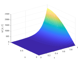
(a) $w(x,t)$.

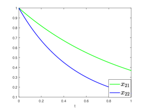
(b) $x_{2}(t)=(x_{21}(t),x_{22}(t))^{\top}$.

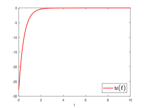
(c) Controller.

Figure 1: Solution of open-loop (7.1) and feedback law.

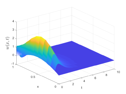
(a) $w(x,t)$.

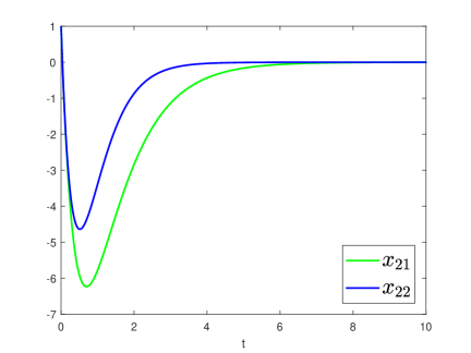
(b) $x_{2}(t)=(x_{21}(t),x_{22}(t))^{\top}$.

Figure 2: Solution of closed-loop (7.19).

9 Conclusions

In this paper, we develop a systematic method to compensate the actuator dynamics dominated by general abstract linear systems. A scheme of full state feedback law design is proposed. As a result, a sufficient condition of the existence of compensator for ODE with PDE actuator dynamics is obtained and the existing results about stabilization of ODE with actuator dynamics dominated by the transport equation [9], wave equation [11], heat equation [10] as well as the Schrödinger equation [19] can be treated in a unified way. More importantly, the more complicated problem that stabilize the infinite-dimensional system through finite-dimensional actuator dynamics can still be addressed effectively. We present two examples to demonstrate the effectiveness of the proposed approach. One is on input delay compensation for ODE system and another is for unstable heat equation with ODE actuator dynamics.

It should be pointed out that the proposed approach in Theorems 5.1 and 5.2 is not limited to the examples considered in Sections 6 and 7. In [34], it has been applied to the stabilization of ODEs with actuator dynamics dominated by Euler-Bernoulli beam equation. More importantly, the approach opens up a new road leading to the stabilization of cascade systems particularly for those systems which consist of ODE and multi-dimensional PDE.

Furthermore, the main idea of the approach is still applicable to the stabilization of PDE-PDE cascade systems like those arising from PDEs with input delay. This will be considered in the third paper [6] of this series works. The present paper focuses only on the full state feedback. After being investigated in the next paper [5] of this series studies for the state observer design through sensor dynamics, the output feedback will become straightforward by the separation principle of the linear systems.

10 Appendix

Lemma 10.1.

Let the operator $A_{1}$ be given by (7.2), $SB_{2}$, $b(\cdot)$ be given by (7.8) and $\phi_{n}(\cdot)$, $\lambda_{n}$ be given by (7.9). Suppose that the integer $N$ satisfies (7.14), $\Lambda_{N}$, $B_{N}$ is given by (7.16) and there exists an $L_{N}=(l_{1},l_{2},\cdots,l_{N})\in\mathcal{L}({\mathbb{R}}^{N},{\mathbb{R}})$ such that $\Lambda_{N}{+}B_{N}L_{N}$ is Hurwitz. Then, the operator $A_{1}+SB_{2}K_{N}$ generates an exponentially stable $C_{0}$-semigroup on $L^{2}[0,1]$, where $K_{N}$ is given by (7.17).

Proof.

Since $A_{1}$ generates an analytic semigroup $e^{A_{1}t}$ on $L^{2}[0,1]$ and $SB_{2}K_{N}$ is bounded, it follows from [18, Corollary 2.3, p.81] that $A_{1}+SB_{2}K_{N}$ also generates an analytic semigroup on $L^{2}[0,1]$. The proof will be accomplished if we can show that $\sigma(A_{1}+SB_{2}K_{N})\subset\{s\ |\ {\rm Re}(s)<0\}$. For any $\lambda\in\sigma(A_{1}+SB_{2}K_{N})$, we consider the characteristic equation $(A_{1}+SB_{2}K_{N})f=\lambda f$ with $f\neq 0$.

When $f\in{\rm Span}\{\phi_{1},\phi_{2},\cdots,\phi_{N}\}$, set $f=\sum_{j=1}^{N}f_{j}\phi_{j}$. The characteristic equation becomes

$$\sum_{j=1}^{N}f_{j}A_{1}\phi_{j}+b\sum_{j=1}^{N}f_{j}K_{N}\phi_{j}=\sum_{j=1}^{N}\lambda f_{j}\phi_{j}.$$ (10.1)

Since $A_{1}\phi_{j}=(-\lambda_{j}+\mu)\phi_{j}$ and

$$K_{N}\phi_{j}=\int_{0}^{1}\phi_{j}(x)\left[\sum_{k=1}^{N}l_{k}\phi_{k}(x)\right]dx=l_{j},\ \ j=1,2,\cdots,N,$$ (10.2)

the equation (10.1) takes the form

$$\sum_{j=1}^{N}f_{j}(-\lambda_{j}+\mu)\phi_{j}+b\sum_{j=1}^{N}f_{j}l_{j}=\sum_{j=1}^{N}\lambda f_{j}\phi_{j}.$$ (10.3)

Take the inner product with $\phi_{n}$, $n=1,2,\cdots,N$ on equation (10.3) to obtain

$$f_{n}(-\lambda_{n}+\mu)+b_{n}\sum_{j=1}^{N}f_{j}l_{j}=\lambda f_{n},\ \ n=1,2,\cdots,N,$$ (10.4)

which, together with (7.16), leads to

$$(\lambda-\Lambda_{N}-B_{N}L_{N})\begin{pmatrix}f_{1}\\ f_{2}\\ \vdots\\ f_{N}\end{pmatrix}=0.$$ (10.5)

Since $(f_{1},f_{2},\cdots,f_{N})\neq 0$, we have

$${\rm Det}(\lambda-\Lambda_{N}-B_{N}L_{N})=0.$$ (10.6)

Hence, $\lambda\in\sigma(\Lambda_{N}{+}B_{N}L_{N})\subset\{s\ |\ {\rm Re}(s)<0\}$ since $\Lambda_{N}{+}B_{N}L_{N}$ is Hurwitz.

When $f\notin{\rm Span}\{\phi_{1},\phi_{2},\cdots,\phi_{N}\}$, there exists a $j_{0}>N$ such that $\displaystyle\int_{0}^{1}f(x)\phi_{j_{0}}(x)dx\neq 0$. Take the inner product with $\phi_{j_{0}}$ on equation $(A_{1}+SB_{2}K_{N})f=\lambda f$ to get

$$(-\lambda_{j_{0}}+\mu)\int_{0}^{1}f(x)\phi_{j_{0}}(x)dx=\lambda\int_{0}^{1}f(x)\phi_{j_{0}}(x)dx,$$ (10.7)

which implies that $\lambda=-\lambda_{j_{0}}+\mu<0$. Therefore, $\lambda\in\sigma(A_{1}+SB_{2}K_{N})\subset\{s\ |\ {\rm Re}(s)<0\}$. The proof is complete. ∎

Lemma 10.2.

Let $A_{j}$ be the generator of a $C_{0}$-semigroup $e^{A_{j}t}$ on $X_{j}$, $j=1,2$. Suppose that $U$ is the control space and $B_{j}\in\mathcal{L}(U,[D(A_{j}^{*})]^{\prime})$ is admissible for $e^{A_{j}t}$, $j=1,2$. Suppose further that $\sigma(A_{1})\cap\sigma(A_{2})=\emptyset$ and system $\left({\rm diag}(A_{1},A_{2}),\begin{pmatrix}B_{1}\\ B_{2}\end{pmatrix}\right)$ is approximately controllable. Then, both $(A_{1},B_{1})$ and $(A_{2},B_{2})$ are approximately controllable.

Proof.

By assumption, system $({\rm diag}(A_{1}^{*},A_{2}^{*}),(B_{1}^{*},B_{2}^{*}))$ is approximately observable. We use the argument of proof by contradiction. If either system $(A_{1},B_{1})$ or $(A_{2},B_{2})$ were not approximately controllable, we assume without loss of the generality that system $(A_{1},B_{1})$ were not approximately controllable. Then, system $(A_{1}^{*},B_{1}^{*})$ would not be approximately observable. Hence, there exists $0\neq x_{10}\in X_{1}$ such that $B_{1}^{*}e^{A_{1}^{*}t}x_{10}\equiv 0$ on $[0,\tau]$ for some time $\tau>0$. As a result, $(B_{1}^{*},B_{2}^{*})e^{{\rm diag}(A_{1}^{*},A_{2}^{*})t}(x_{10},0)^{\top}\equiv 0$ over $[0,\tau]$, that is, ${\rm Ker}\left((B_{1}^{*},B_{2}^{*})e^{{\rm diag}(A_{1}^{*},A_{2}^{*})t}\right)\neq\{0\}$. This contradicts to the fact that system $({\rm diag}(A_{1}^{*},A_{2}^{*}),(B_{1}^{*},B_{2}^{*}))$ is approximately observable. The proof is complete. ∎

References

- [1] Z. Artstein, Linear systems with delayed controls: A reduction, IEEE Transactions on Automatic Control, 27(1982), 869-879.
- [2] J.M. Coron and E. Trélat, Global steady-state controllability of one dimensional semilinear heat equations, SIAM Journal on Control and Optimization, 43(2004), 549-569.
- [3] H. Feng, B.Z. Guo and X.H. Wu, Trajectory planning approach to output tracking for a 1-d wave equation, IEEE Transactions on Automatic Control, 65(2020), 1841-1854.
- [4] H. Feng and B.Z. Guo, A new active disturbance rejection control to output feedback stabilization for a one-dimensional anti-stable wave equation with disturbance, IEEE Transactions on Automatic Control, 62(2017), 3774-3787.
- [5] H. Feng, X.H. Wu and B.Z. Guo, Dynamics compensation in observation of abstract linear systems, to be submitted ( as the second part of this series of studies).
- [6] H. Feng, Delays compensations for regular linear systems, to be submitted ( as the third part of this series of studies).
- [7] H. Feng and B.Z. Guo, Extended dynamics observer for linear systems with disturbance, to be submitted ( as the last part of this series of studies).
- [8] W.H. Kwon and A.E. Pearson, Feedback stabilization of linear systems with delayed control, IEEE Transactions on Automatic Control, 25(1980), 266-269.
- [9] M. Krstic and A. Smyshlyaev, Backstepping boundary control for first order hyperbolic PDEs and application to systems with actuator and sensor delays, Systems Control Letters, 57(2008), 750-758.
- [10] M. Krstic, Compensating actuator and sensor dynamics governed by diffusion PDEs, Systems Control Letters, 58(2009), 372-377.
- [11] M. Krstic, Compensating a string PDE in the actuation or in sensing path of an unstable ODE, IEEE Transactions on Automatic Control, 54(2009), 1362-1368.
- [12] A.Z. Manitius and A.W. Olbrot, Finite spectrum assignment problem for systems with delays, IEEE Transactions on Automatic Control, 24(1979), 541-553.
- [13] N.J. Higham, Functions of Matrices Theory and Computation, SIAM, Philadelphia, 2008.
- [14] L. Paunonen, The role of exosystems in output regulation, IEEE Transactions on Automatic Control, 59(2014), 2301-2305.
- [15] L. Paunonen and S. Pohjolainen, The internal model principle for systems with unbounded control and observation, SIAM Journal on Control and Optimization, 52(2014), 3967-4000.
- [16] V.Q. Phóng, The operator equation with unbounded operators and and related abstract Cauchy problems, Mathematische Zeitschrift, 208(1991), 567-588.
- [17] C. Prieur and E. Trélat, Feedback stabilization of a 1-d linear reaction-diffusion equation with delay boundary control, IEEE Transactions on Automatic Control, 64(2019), 1415-1425.
- [18] A. Pazy, Semigroups of Linear Operators and Applications to Partial Differential Equations, Springer-Verlag, New York, 1983.
- [19] B. Ren, J.M. Wang and M. Krstic, Stabilization of an ODE-Schrödinger cascade, Systems Control Letters, 62(2013), 503-510.
- [20] M. Rosenblum, On the operator equation , Duke Mathematical Journal, 23(1956), 263-270.
- [21] D.L. Russell, Controllability and stabilizability theory for linear partial differential equations: recent progress and open questions, SIAM Review, 20(1978), 639-739.
- [22] D. Salamon, Infinite-dimensional systems with unbounded control and observation: a functional analytic approach, Transactions of American Mathematical Society, 300(1987), 383-431.
- [23] G.A. Sustoa and M. Krstic, Control of PDE-ODE cascades with Neumann interconnections, Journal of the Franklin Institute, 347(2010), 284-314.
- [24] O.J. M. Smith, A controller to overcome dead time, ISA J, 6(1959), 28-33.
- [25] S. Tang and C. Xie, State and output feedback boundary control for a coupled PDE-ODE system, Systems Control Letters, 60(2011), 540-545.
- [26] J.W. Thomas, Numerical Partial Differential Equations: Conservation Laws and Elliptic Equations, Springer-Verlag, New York, 1999.
- [27] M. Tucsnak and G. Weiss, Observation and Control for Operator Semigroups, Birkhäuser, Basel, 2009.
- [28] J.M. Wang, J.J. Liu, B. Ren and J. Chen. Sliding mode control to stabilization of cascaded heat PDE-ODE systems subject to boundary control matched disturbance, Automatica, 52(2015), 23-34.
- [29] G. Weiss, Admissibility of unbounded control operators, SIAM Journal on Control and Optimization, 27(1989), 527-545.
- [30] G. Weiss, Regular linear systems with feedback, Mathematics of Control, Signals, and Systems, 7(1994), 23-57.
- [31] G. Weiss, Admissible observation operators for linear semigroups, Israel Journal of Mathematgics, 65(1989), 17-43.
- [32] G. Weiss and R. Curtain, Dynamic stabilization of regular linear systems, IEEE Transactions on Automatic Control, 42(1997), 4-21.
- [33] J. Weidmann, Linear Operators in Hilbert Spaces, Springer-Verlag, New York, 1980.
- [34] X.H. Wu and H. Feng, Exponential stabilization of ODE system with Euler-Bernoulli beam actuator dynamics, SCIENCE CHINA Information Sciences, to appear.
- [35] H.C. Zhou and B.Z. Guo, Unknown input observer design and output feedback stabilization for multi-dimensional wave equation with boundary control matched uncertainty, Journal of Differential Equations, 263(2017), 2213-2246.