Variance-Reduced Splitting Schemes for Monotone Stochastic Generalized Equations

Abstract

We consider monotone inclusion problems where the operators may be expectation-valued, a class of problems that subsumes convex stochastic optimization problems as well as subclasses of stochastic variational inequality and equilibrium problems. A direct application of splitting schemes is complicated by the need to resolve problems with expectation-valued maps at each step, a concern that is addressed by using sampling. Accordingly, we propose an avenue for addressing uncertainty in the mapping: Variance-reduced stochastic modified forward-backward splitting scheme (vr-SMFBS). In constrained settings, we consider structured settings when the map can be decomposed into an expectation-valued map $A$ and a maximal monotone map $B$ with a tractable resolvent. We show that the proposed schemes are equipped with a.s. convergence guarantees, linear (strongly monotone $A$) and $\mathcal{O}(1/k)$ (monotone $A$) rates of convergence while achieving optimal oracle complexity bounds. The rate statements in monotone regimes appear to be amongst the first and rely on leveraging the Fitzpatrick gap function for monotone inclusions. Furthermore, the schemes rely on weaker moment requirements on noise and allow for weakening unbiasedness requirements on oracles in strongly monotone regimes. Preliminary numerics on a class of two-stage stochastic variational inequality problems reflect these findings and show that the variance-reduced schemes outperform stochastic approximation schemes and sample-average approximation approaches. The benefits of attaining deterministic rates of convergence become even more salient when resolvent computation is expensive.

I Introduction

The generalized equation (alternately referred to as the inclusion problem) represents a crucial mathematical object in decision and control theory, representing a set-valued generalization to the more standard root-finding problem which requires solving $F(x)=0$, where $F:\mathbb{R}^{n}\to\mathbb{R}^{n}$ is single-valued. Specifically, if $T$ is a set-valued map, defined as $T:\mathbb{R}^{n}\rightrightarrows\mathbb{R}^{n}$, and $T$ is characterized by a distinct structure in that it can be cast as the sum of two operators $A$ and $B$, then the generalized equation (GE) takes the form

$$0\in T(x)\triangleq A(x)+B(x).$$ (GE)

Here $A:\mathbb{R}^{n}\to\mathbb{R}^{n}$ is a single-valued map and $B:\mathbb{R}^{n}\rightrightarrows\mathbb{R}^{n}$ is a set-valued map. While such objects have a storied history, an excellent overview was first provided by Robinson [1]. Generalized equations have been extensively examined since the 70s when Rockafellar [2] developed a proximal point scheme for a generalized equation characterized by monotone operators. In fact, this scheme subsumes a range of well known schemes such as the augmented Lagrangian method [3], Douglas-Rachford splitting [4], amongst others. It can be observed that a large class of optimization and equilibrium problems can be modeled as (GE), including the necessary conditions of nonlinear programming problems, variational inequality and complementarity problems, and a broad range of equilibrium problems (cf. [1]). Under suitable requirements on $A$ and $B$, a range of splitting methods can be developed and has represented a vibrant area of research over the last two decades [4, 5, 6, 7].

In this paper, we consider addressing the stochastic counterpart of generalized equations, a class of problems that has seen recent study via sample-average approximation (SAA) techniques [8]. Formally, the stochastic generalized equation requires an $x\in\mathbb{R}^{n}$ such that

$$0\in\mathbb{E}[T(x,\xi(\omega))]\triangleq\mathbb{E}[A(x,\xi(\omega))]+B(x),$$ (SGE)

where the components of the map $A$ are denoted by $A_{i}$, $i=1,\dots,n$, $\xi:\Omega\to\mathbb{R}^{d}$ is a random variable, $A_{i}:\mathbb{R}^{n}\times\Omega\rightrightarrows\mathbb{R}^{n}$ is a set-valued map, $\mathbb{E}[\cdot]$ denotes the expectation, and the associated probability space is given by $(\Omega,{\cal F},\mathbb{P})$. In the remainder of this paper, we refer to $A(x,\xi(\omega))$ by $A(x,\omega)$. The expectation of a set-valued map leverages the Aumann integral [9] and is formally defined as $\mathbb{E}[A_{i}(x,\xi(\omega))]=\left\{\int v_{i}(\omega)dP(\omega)\mid\quad v_{i}(\omega)\in A_{i}(x,\xi(\omega))\right\}.$ Consequently, the expectation $\mathbb{E}[A(x,\omega)]$ can be defined as a Cartesian product of the sets $\mathbb{E}[A_{i}(x,\omega)]$, defined as $\mathbb{E}[A(x,\omega)]\ \triangleq\ \prod_{i=1}^{n}\mathbb{E}[A_{i}(x,\omega)].$ We motivate (SGE) by considering some examples. Consider the stochastic convex optimization problem [10, 11, 12] given by ${\displaystyle\min_{x\in\mathcal{X}}}\,\mathbb{E}[g(x,\omega)],$ where $g(\bullet,\omega)$ is a differentiable convex function for every $\omega$ and $\mathcal{X}$ is a closed and convex set. Such a problem can be equivalently stated as $0\in T(x)\triangleq\mathbb{E}[G(x,\omega)]+\mathcal{N}_{\mathcal{X}}(x)$, where $G(x,\omega)=\nabla g(x,\omega)$ and $\mathcal{N}_{\mathcal{X}}(x)$ denotes the normal cone of $\mathcal{X}$ at $x$. In fact, the single-valued stochastic variational inequality problems [13, 14, 15] can be cast as stochastic inclusions as well as seen by $0\in T(x)\triangleq\mathbb{E}[F(x,\omega)]+\mathcal{N}_{\mathcal{X}}(x)$, where $F(\bullet,\omega)$ is a realization of the mapping. This introduces a pathway for examining stochastic analogs of traffic equilibrium [16] and Nash equilibrium problems [17] as well as a myriad of other problems subsumed by variational inequality problems [18]. We describe two problems that have seen recent study which can also be modeled as SGEs, allowing for developing new computational techniques.

I-A Two motivating examples

(a) A subclass of stochastic multi-leader multi-follower games. Consider a class of multi-leader multi-follower games [19, 20, 21, 22] with ${\bf N}$ leaders, denoted by $\{1,\cdots,{\bf N}\}$ and $M$ followers, given by $\{1,\cdots,{\bf M}\}.$ In general, this class of games is challenging to analyze since the player problems are nonconvex and early existence statements have relied on eliminating follower-level decisions, leading to a noncooperative game with convex nonsmooth player problems. Adopting a similar approach in examining a stochastic generalization of a quadratic setting examined in [23] with a single follower where ${\bf M}=1$, suppose the follower problem is

$$\min_{y_{i}\,\geq\,l_{i}(x_{i})} \quad\tfrac{1}{2}y_{i}^{\mathsf{T}}Q_{i}y_{i}-b_{i}(x_{i})^{\mathsf{T}}y_{i}, {}_{i}(x_{i})$$ (Follow)

where $Q_{i}$ is a positive definite and diagonal matrix, $b_{i}(\bullet)$ and $l_{i}(\bullet)$ are affine functions. Suppose the leaders compete in a Cournot game in which the $i$th leader solves

$$\min_{x_{i}\,\in\,\mathcal{X}_{i}} \quad c_{i}(x_{i})-\mathbb{E}[p(X,\omega)x_{i}]+a_{i}y_{i}(x_{i}), {}_{i}(x_{-i})$$ (Leader)

where $c_{i}:\mathcal{X}_{i}\to\mathbb{R}$ is a smooth convex function, the inverse-demand function $p(\bullet)$ is defined as $p(X)\triangleq d(\omega)-r(\omega)X$, $d(\omega),r(\omega)>0$ for every $\omega\in\Omega$, $X\triangleq\sum_{i=1}^{N}x_{i}$, $y_{i}(x_{i})$ denotes a best-response of follower $i$, and $\mathcal{X}_{i}$ is a closed and convex set in $\mathbb{R}$. Follower $i$’s best-response $y_{i}(x)$, given leader-level decisions $x$, can be derived by considering the necessary and sufficient conditions of optimality:

$$y_{i}(x_{i})=\max\{Q_{i}^{-1}b_{i}(x_{i}),l_{i}(x_{i})\}.$$

Consequently, we may eliminate the follower-level decision in the leader level problem, leading to a nonsmooth stochastic Nash equilibrium problem given by the following:

$$\begin{aligned} \min_{x_{i}\in\mathcal{X}_{i}}&c_{i}(x_{i})-\mathbb{E}[p(X,\omega)x_{i}]\\ &+{a_{i}^{\mathsf{T}}\max\{Q_{i}^{-1}b_{i}(x_{i}),l_{i}(x_{i})\}}.\end{aligned} {}_{i}(x_{-i})$$ (Leader)

Under convexity of $b_{i}(\bullet)$ and $l_{i}(\bullet)$, and suitable assumptions on $Q_{i}$ and $a_{i}$, the expression $a_{i}^{\mathsf{T}}\max\{Q_{i}^{-1}b_{i}(x_{i}),l_{i}(x_{i})\}$ is a convex function in $x_{i}$, a fact that follows from observing that this term is a scaling of the maximum of two convex functions. Consequently, the necessary and sufficient equilibrium conditions of this game are given by $0\in\nabla_{x_{i}}c_{i}(x_{i})+\mathbb{E}[r(\omega)(X+x_{i})-d(\omega)]+\partial_{x_{i}}h_{i}(x_{i})+\mathcal{N}_{\mathcal{X}_{i}}(x_{i})$ for $i=1,\ldots,{\bf N}$ where $h_{i}(\bullet)$, defined as $h_{i}(x_{i})\triangleq a_{i}^{\mathsf{T}}\max\{Q_{i}^{-1}b_{i}(x_{i}),l_{i}(x_{i})\}$, is a convex function in $x_{i}$. Then the necessary and sufficient equilibrium conditions are given by

$$0 \in T(x)\triangleq A(x)+B(x),$$ (SGE_mlf)

$$\mbox{ where }A(x) \triangleq G(x)+R(x),B(x)\triangleq D(x)+\mathcal{N}_{\mathcal{X}}(x).$$

Here $G(x)\triangleq(c_{i}^{\prime}(x_{i}))_{i=1}^{N}$, $R(x)\triangleq\mathbb{E}[r(\omega)(X{\bf 1}+x)-d(\omega){\bf 1}]$ and $D(x)\triangleq\mathbb{E}[\partial_{x_{i}}h_{i}(x_{i})]$. We observe that $G$ is a monotone map while $D(x)$ is the Cartesian product of the expectations of subdifferentials of convex functions, implying that $D$ is also monotone. Furthermore, $R$ is monotone since $\nabla_{x}R(x)=\mathbb{E}[r(\omega)(\mathbf{I}+{\bf 1}{\bf 1}^{\mathsf{T}})]\succeq 0.$ Since $\mathcal{N}_{\mathcal{X}}$ is a normal cone of a convex set, it is also a monotone map, implying that $T$ is monotone.

(b) Model predictive control (MPC) with probabilistic and risk constraints. Model-predictive control (MPC) is a framework for the control of complex systems [24]. It obviates the challenging derivation/computation of a feedback control law with repeated resolution of a finite-horizon constrained optimization problem. Contending with uncertainty has prompted the development of several approaches: (i) Robust approaches. Robust frameworks for MPC [25, 26, 27, 28, 29, 30] often require bounded and deterministic descriptions of uncertainty, a property inherited from robust optimization [31]; (ii) Probabilistic framework. Under a probabilistic representation of the uncertainty, chance-constrained MPC framework [32, 33, 34, 35, 36, 37] can be adopted, allowing for shaping the probability distribution of system states. Such avenues have assumed relevance in settings such as climate control, process control, power systems operation, and vehicle path planning (cf. [38] for an excellent survey). Suppose the dynamics are captured by a linear discrete-time system, defined as

$${\mathbf{x}}_{t+1}=A(\delta){\mathbf{x}}_{t}+B_{u}(\delta){\mathbf{u}}_{t}+B_{w}(\delta){\mathbf{w}}_{t},$$ (1)

where ${\mathbf{x}}_{0}$ is given, ${\mathbf{x}}_{t}\in{\cal X}$ denotes the state of the system at time $k$, ${\mathbf{u}}_{t}\in{\cal U}\subseteq\mathbb{R}^{m}$ represents the control input vector at time $t$, and ${\mathbf{w}}_{t}\in\mathbb{R}^{p}$ is an unmeasurable disturbance signal at time $t$. In addition, ${\cal X}$ and ${\cal U}$ represent the set of states and controls, respectively while the random matrices $A(\delta),B_{u}(\delta),B_{w}(\delta)$ lie in $\mathbb{R}^{n\times n},\mathbb{R}^{n\times m}$, and $\mathbb{R}^{n\times p}$, respectively. We assume access to the distributions governing $\delta$ and ${\mathbf{w}}_{k}$. Suppose ${\color[rgb]{0,0,0}{{\boldsymbol{\pi}}}}\triangleq\{\pi_{0}(\cdot),\cdots,\pi_{N-1}(\cdot)\}$ represents feedback-control policy where $\pi_{i}:\mathbb{R}^{n}\to\mathcal{U}\subseteq\mathbb{R}^{m}$ denotes the state feedback control law for $i=0,1,\cdots,N-1$. We may then formally define the value function $\mathcal{V}_{N}$ as $\mathcal{V}_{N}({\mathbf{x}},{\color[rgb]{0,0,0}{{\boldsymbol{\pi}}}})\triangleq\mathbb{E}_{{\mathbf{x}}_{0}}\left[\sum_{i=1}^{N}J({\mathbf{x}}_{i},{\mathbf{u}}_{i})+J_{N}({\mathbf{x}}_{N})\right]$ where $\mathbb{E}_{{\mathbf{x}}_{0}}[\bullet]\triangleq\mathbb{E}[\bullet\mid{\mathbf{x}}_{0}].$ In addition, suppose ${\cal X}_{c}$ denotes a set of undesirable outcomes. The resulting chance-constrained stochastic control problem requires determining the feedback-control law ${\color[rgb]{0,0,0}{{\boldsymbol{\pi}}}}$ that minimizes $\mathcal{V}_{N}({\mathbf{x}},{\color[rgb]{0,0,0}{{\boldsymbol{\pi}}}})$ subject to the prescribed dynamics and probabilistic requirements on the state. This problem is challenging, motivating the construction of a finite-horizon open-loop counterpart. To this end, we define ${\mathbf{x}}_{t,T}$ and ${\mathbf{u}}_{t,T}$ as ${\mathbf{x}}_{t,T}\triangleq\{{\mathbf{x}}_{t},\cdots,{\mathbf{x}}_{t+T-1)}\}$ and ${\mathbf{u}}_{t,T}\triangleq\{{\mathbf{u}}_{t},\cdots,{\mathbf{u}}_{t+T-1)}\}$, respectively while the finite-horizon value function at the $t$-th step looking $T$ periods ahead, denoted by $\mathcal{V}_{t,T}({\mathbf{x}}_{t,T},{\mathbf{u}}_{t,T})$, is defined as $\mathcal{V}_{t,T}({\mathbf{x}}_{t,T},{\mathbf{u}}_{t,T})\triangleq\mathbb{E}_{{\mathbf{x}}_{t}}\left[\sum_{i=t+1}^{T}J({\mathbf{x}}_{i},{\mathbf{u}}_{i})\right]$ where $T\ll N$. Given a horizon $T$, the resulting MPC framework [39] requires minimizing $\mathcal{V}_{t,T}({\mathbf{x}}_{t,T},{\mathbf{u}}_{t,T})$ subject to the prescribed dynamics and the probabilistic state-constraints, given ${\mathbf{x}}_{t}$. A formal definition of the chance-constrained stochastic control problem (CC-SC) and its finite-horizon counterpart (CC-MPC${}_{t}^{T}$) is provided next.

$$\framebox{$\begin{aligned} &\ \mbox{\bf(CC-SC)}\max_{{\color[rgb]{0,0,0}{{\boldsymbol{\pi}}}},{\mathbf{x}}}\ \mathcal{V}_{N}({\mathbf{x}},{\color[rgb]{0,0,0}{{\boldsymbol{\pi}}}})\\ \mbox{s.t.}&\ \mathbb{P}_{{\mathbf{x}}_{0}}\left\{\omega:{\mathbf{x}}_{i}\in{\cal X}_{c},\forall i\in[1;N]\right\}\leq\epsilon\\ &\ \text{ where ${\mathbf{x}}_{k}$ evolves as per \eqref{eq:linear_system}}.\end{aligned}$}\ \framebox{$\begin{aligned} &\,\mbox{\bf(CC-MPC${}_{t}^{T}$)}\ \max_{\tiny{\mathbf{u}}_{t,T},{\mathbf{x}}_{t,T}}\ \mathcal{V}_{t,T}({\mathbf{x}}_{t,T},u_{t,T})\\ \mbox{s.t.}&\ \mathbb{P}_{{\mathbf{x}}_{t}}\left\{\omega:{\mathbf{x}}_{i}\in{\cal X}_{c},\forall i\in[k;T]\right\}\leq\epsilon\\ &\ \text{ where ${\mathbf{x}}_{t}$ evolves as per \eqref{eq:linear_system}}\end{aligned}$}.$$

The control decision ${\mathbf{u}}_{t}$ is obtained from resolving (CC-MPC_t,T) and is then applied to the system after which the window is moved ahead. The resulting problem (CC-MPC_t+1,T) is then resolved when $t+T<N$ (alternately, the horizon $T$ is reduced appropriately). This formulation is relatively flexbile and and can be used to address diverse types of objectives and constraints. In general, the problem (CC-MPC${}_{t}^{T}$) is challenging, owing to the presence of the chance constraint. The probability function can be recast as an expectation of an indicator function over a set but this leads to discontinuous integrands. Recently, the second author has developed avenues where under prescribed assumptions under which the following holds [40].

$$\mathbb{P}\left[\zeta\in\mathcal{K}\mid\zeta\in{\bf K}({\mathbf{x}})\right]=\mathbb{E}_{\xi}\left[F({\mathbf{x}},\xi)\right],$$ (2)

where $\mathcal{K}$ is a set in $\mathbb{R}^{n}$ symmetric about the origin, ${\bf K}({\mathbf{x}})$ is defined as ${\bf K}({\mathbf{x}})\triangleq\{\zeta:c({\mathbf{x}},\zeta)\geq 0\}$, $T\in\mathbb{R}^{d\times n}$, and

$$c({\mathbf{x}},\zeta)\triangleq\left\{\begin{aligned} &1-|\zeta^{\mathsf{T}}{\mathbf{x}}|^{m},\quad\mbox{Setting A}\\ &T{\mathbf{x}}-\zeta.\quad\qquad\mbox{Setting B}\end{aligned}\right.$$

The integrand $F(\bullet,\xi)$ is defined appropriately in Settings A and B where in each case, it is shown that $\xi$. In fact, we can then show that a composition of $\mathbb{E}[F(\bullet,\xi)]$ is convex; e.g. in Setting A, $1/\mathbb{E}[F(\bullet,\xi)]$ is convex. For expository ease, we may recast (CC-MPC${}_{t}^{T}$) as the following chance-constrained problem (CCP) and provide its necessary and sufficient optimality conditions in (SGE_ccp).

$$\framebox{$\begin{aligned} &\ \mbox{\bf(CCP)}\min_{{\mathbf{x}}}\mathbb{E}_{\omega}[h({\mathbf{x}},\omega)]\\ &\mbox{s.t.}\ g({\mathbf{x}})\leq 0,\quad(\lambda)\end{aligned}$}\quad\overset{\mbox{(Reg. conds)}}{\equiv}\quad\framebox{$\begin{aligned} &\,\mbox{\bf(SGE${}_{\rm ccp}$)}\quad\mbox{Find ${\mathbf{z}}\triangleq(x,\lambda)$ such that}\\ &0\in T({\mathbf{z}})\triangleq H({\mathbf{z}})+\mathcal{N}_{\mathcal{Z}}({\mathbf{z}}),\end{aligned}$}.$$

where $g({\mathbf{x}})\triangleq\tfrac{1}{\mathbb{E}_{\xi}[F({\mathbf{x}},\xi)]}-\tfrac{1}{(1-\epsilon)}$, $\mathcal{Z}\triangleq\mathcal{X}\times\mathbb{R}^{+}_{m}$, $\mathcal{N}_{\mathcal{Z}}(z)$ denotes normal cone of $\mathcal{Z}$ at $z$, $H$ is a monotone set-valued map defined as

$$H({\mathbf{x}},\lambda)\triangleq\left\{\nabla_{x}f({\mathbf{x}})+\lambda\partial_{x}g({\mathbf{x}})\right\}\times\{g({\mathbf{x}})\}.$$

We close by noting that monotone inclusions with expectation-valued operators are of crucial relevance in decision and control problems, providing a strong motivation for addressing their tractable resolution.

I-B Related work.

We provide a brief review of prior research.

TABLE I: Variance-reduced vs Stochastic operator-splitting schemes for SGEs

Alg/Prob.	$A,B$	Biased	$\gamma_{k}$; $N_{k}$	Statements
[41]	$L_{A}$, MM	N	SS, NS; 1	$x_{k}\xrightarrow[a.s]{k\to\infty}x^{*}\in\mathcal{X}^{*}$
[41]	$L_{A}$, $\sigma_{A}$, $\mu_{B}$	N	SS, NS; 1	$\mathbb{E}[\|x_{k}-x^{*}\|^{2}]\leq\mathcal{O}(1/k)$
[42]	$L_{A}$, MM	N	SS, NS; 1	$x_{k}\xrightarrow[a.s]{k\to\infty}x^{*}\in\mathcal{X}^{*}$
(vr-SMFBS)	$\sigma_{A}$, MM	Y	$\gamma$;$\lfloor\rho^{-(k+1)}\rfloor$ $\rho<1$	$x_{k}\xrightarrow[a.s]{k\to\infty}x^{*}$ $\mathbb{E}[\|x_{k}-x^{*}\|^{2}]\leq\mathcal{O}(q^{k})$ Sample-complexity: $\mathcal{O}(1/\epsilon)$
(vr-SMFBS)	$L_{A}$, MM	N	$\gamma$;$\lfloor k^{a}\rfloor$ $a>1$	$x_{k}\xrightarrow[a.s]{k\to\infty}x^{*}\in\mathcal{X}^{*}$ $\mathbb{E}[G(\bar{x}_{k})]\leq\mathcal{O}(1/k)$ Sample-complexity: $\mathcal{O}(1/\epsilon^{2+\delta})$

• $L_{A}$: Lipschitz constant of $A$, MM: Maximal monotone

• $\sigma_{A},\mu_{B}$: strong monotonicity constants of $A$ and $B$

• SS: square-summable, NS: non-summable

(a) Stochastic operator splitting schemes. The regime where the maps are expectation-valued has seen relatively less study [43]. Stochastic proximal gradient schemes [44, 45, 46, 47, 48] are an instance of stochastic operator splitting techniques where $A$ is either the gradient or the subdifferential operator. In the context of monotone inclusions, when $A$ is a more general monotone operator, a.s. convergence of the iterates has been proven in  [42] and  [41] when $A$ is Lipschitz and expectation-valued while $B$ is maximal monotone. In fact, in our prior work [49], we prove a.s. convergence and derive an optimal rate in terms of the gap function in the context of stochastic variational inequality problems with structured operators. Stability analysis [50] and two-timescale variants [51] have also been examined. A rate statement of $\mathcal{O}(\tfrac{1}{k})$ in terms of mean-squared error has also been provided when $A$ is additionally strongly monotone in [41]. A more general problem which finds a zero of the sum of three maximally monotone operators is proposed in [52]. A comparison of rate statements for stochastic operator-splitting schemes is provided in Table I from which we note that (vr-SMBFS) is equipped with deterministic (optimal) rate statements, optimal or near-optimal sample-complexity, a.s. convergence guarantees, and does not require imposing a conditional unbiasedness requirement on the oracle in the strongly monotone regime. We believe our rate statements are amongst the first in maximal monotone settings (to the best of our knowledge).

(b) Other related schemes. A natural approach for resolving SGEs is via sample-average approximation [53, 54]. It proves the weak a.s. convergence and establishes the rate of convergence in expectation under strong monotonicity assumption.

I-C Gaps and resolution.

1. Poorer empirical performance when resolvents are costly. Deterministic schemes for strongly monotone and monotone generalized equations display linear and $\mathcal{O}(1/k)$ rate in resolvent operations while stochastic analogs display rates of $\mathcal{O}(1/k)$ and $\mathcal{O}(1/\sqrt{k})$, respectively. This leads to far poorer practical behavior particularly when the resolvent is challenging to compute, e.g., in strongly monotone regimes, the complexity in resolvent operations can increase from $\mathcal{O}(\log(1/\epsilon))$ to $\mathcal{O}(1/\epsilon)$. The proposed scheme (vr-SMBFS) achieve deterministic rates of convergence with either identical or slightly worse oracle complexities in both monotone and strongly monotone regimes, allowing for run-times comparable to deterministic counterpart.

2. Absence of rate statements for monotone operators. To the best of our knowledge, there appear to be no non-asymptotic rate statements available in monotone regimes. In (vr-SMBFS), rate statements are now provided.

3. Biased oracles. In many settings, conditional unbiasedness of the oracle may be harder to impose and one may need to impose weaker assumptions. Our proposed scheme allows for possibly biased oracles in some select settings.

4. State-dependent bounds on subgradients and second moments. Many subgradient and stochastic approximation schemes impose bounds of the form $\mathbb{E}[\|G(x,\omega)\|^{2}]\leq M^{2}$ where $G(x,\omega)\in T(x,\omega)$ or $\mathbb{E}[\|w\|^{2}\mid x]\leq\nu^{2}$ where $w=\nabla_{x}f(x,\omega)-\nabla_{x}f(x)$. Both sets of assumptions are often challenging to impose non-compact regimes. Our scheme can accommodate state-dependent bounds to allow for non-compact domains.

I-D Outline and contributions.

We now articulate our contributions. In Section III, we consider the resolution of monotone inclusions in structured regimes where the map can be expressed as the sum of two maps, facilitating the use of splitting. In this context, when one of the maps is expectation-valued while the other has a cheap resolvent, we consider a scheme where a sample-average of the expectation-valued map is utilized in the forward step. When the sample-size is increased at a suitable rate, the sequence of iterates is shown to converge a.s. to a solution of the constrained stochastic generalized equation in both monotone and strongly monotone regimes. In addition, the resulting sequence of iterates converges either at a linear rate (strongly monotone) or at a rate of $\mathcal{O}(1/k)$ (maximal monotone), leading to optimal oracle complexities of $\mathcal{O}(1/\epsilon)$ and $\mathcal{O}(1/\epsilon^{2+\delta})$ ($\delta>0$), respectively. Notably, the strong monotonicity claim is made without an unbiasedness requirement on the oracle while weaker state-dependent noise requirements are assumed througout. Rate statements in maximally monotone regimes rely on using the Fitzpatrick gap function for inclusion problems. We believe that the rate statements in monotone regimes are amongst the first. In addition, we provide some background in Section II while preliminary numerics are presented in Section IV.

I-E Comments on variance-reduced schemes.

Before proceeding, we briefly digress regarding the term variance-reduced.

(i) Terminology and applicability. The moniker “variance-reduced” reflects the usage of increasing accurate approximations of the expectation-valued map, as opposed to noisy sampled variants that are used in single sample schemes. The resulting schemes are often referred to as mini-batch SA schemes and often achieve deterministic rates of convergence. This work draws inspiration from the early work by Friedlander and Schmidt [55] and Byrd et al. [56] which demonstrated how increasing sample-sizes can enable achieving deterministic rates of convergence. Similar findings regarding the nature of sampling rates have been presented in [57]. This avenue has proven particularly useful in developing accelerated gradient schemes for smooth [47, 58] and nonsmooth [46] convex/nonconvex stochastic optimization, variance-reduced quasi-Newton schemes [59, 60], amongst others. Schemes such as SVRG [61] and SAGA [62] also achieve deterministic rates of convergence but are customized for finite sum problems unlike mini-batch schemes that can process expectations over general probability spaces. Unlike in mini-batch schemes where increasing batch-sizes are employed, in schemes such as SVRG, the entire set of samples is periodically employed for computing a step.

(ii) Weaker assumptions and stronger statements. The proposed variance-reduced framework has several crucial benefits that can often not be reaped in the single-sample regime. For instance, rate statements are derived in monotone regimes which have hitherto been unavailable. Second, a.s. convergence guarantees are obtained and in some cases require far weaker moment assumptions. Finally, since the schemes allow for deterministic rates, this leads to far better practical behavior as the numerics reveal.

(iii) Sampling requirements. Naturally, variance-reduced schemes can generally be employed only when sampling is relatively cheap compared to the main computational step (such as computing a projection or a prox.) In terms of overall sample-complexity, the proposed schemes are near optimal. As $k$ becomes large, one might question how one might contend with $N_{k}$ tending to $+\infty$. This issue does not arise since most schemes of this form are meant to provide $\epsilon$-approximations. For instance, if $\epsilon=10^{-3}$, then such a scheme requires approximately $\mathcal{O}(10^{3})$ steps (in monotone settings). Since $N_{k}\approx\lfloor k^{a}\rfloor$ and $a>1$, we require approximately $(\mathcal{O}(10^{3}))^{1+a}$ samples in total. In a setting where multi-core architecture is ubiquitous, such requirements are not terribly onerous particularly since computational costs have been reduced from $\mathcal{O}(10^{6})$ (single-sample) to $\mathcal{O}(10^{3})$. It is worth noting that finite-sum problems routinely have $10^{9}$ or more samples and competing schemes such as SVRG would require taking the full batch-size intermittently, which means they use $\mathcal{O}(10^{9})$ samples at least to achieve the same accuracy as our scheme.

II Background

In this section, we provide some background on splitting schemes, building a foundation for the subsequent sections.
Consider the generalized equation

$$0\in T(x)\triangleq A(x)+B(x).$$ (GE)

If the resolvent of either $A$ or $B$ (or both) is tractable, then splitting schemes assume relevance. Notable instances include Douglas-Rachford splitting [4, 6], Peaceman-Rachford splitting [5, 6], and Forward-Backward splitting (FBS) [6, 7]. (a) Douglas-Rachford Splitting [4, 6]. In this scheme, the resolvent of $A$ and $B$ can be separately evaluated to generate a sequence defined as follows.

$$\begin{aligned} x_{k+\frac{1}{2}}&\coloneqq(\mathbf{I}+\gamma A)^{-1}(x_{k})\\ x_{k+1}&\coloneqq(\mathbf{I}+\gamma B)^{-1}(2x_{k+\frac{1}{2}}-x_{k})+x_{k}-x_{k+\frac{1}{2}}.\end{aligned}$$ (DRS)

(b) Peaceman-Rachford Splitting [5, 6]. In contrast, in the Peaceman-Rachford splitting method, the the roles of $A$ and $B$ are exchanged in each iteration, given by the following.

$$\begin{aligned} x_{k+\frac{1}{2}}&\coloneqq(\mathbf{I}+\gamma B)^{-1}(\mathbf{I}-\gamma A)(x_{k}),\\ x_{k+1}&\coloneqq(\mathbf{I}+\gamma A)^{-1}(\mathbf{I}-\gamma B)(x_{k+\frac{1}{2}}).\end{aligned}$$

(c) Forward-backward splitting [6, 7]. Moreover, if the resolvent of $B$ is easier to evaluate and $A$ and $B$ are maximal monotone, the forward-backward splitting method [6, 7] was applied to convex optimization in [63]:

$$x_{k+1}\coloneqq(\mathbf{I}+\gamma B)^{-1}(\mathbf{I}-\gamma A)(x_{k}).$$

In [42], a stochastic variant of the FBS method, developed for strongly monotone maps, is equipped with a rate of $\mathcal{O}(1/k)$ while in [41], maximal monotone regimes are examined and a.s. convergence statements are provided. A drawback of (FBS) is the requirement of either a strong monotonicity assumption on $A^{-1}$, or that $A$ be Lipschitz continuous on $\mbox{dom}(A)=\mathbb{R}^{n}$ and $T$ be strongly monotone; this motivated the modified FBS scheme where convergence was proven when $A$ is monotone and Lipschitz [64].

$$\begin{aligned} x_{k+\frac{1}{2}}&\coloneqq(\mathbf{I}+\gamma B)^{-1}(\mathbf{I}-\gamma A)(x_{k}),\\ x_{k+1}&\coloneqq x_{k+\frac{1}{2}}-\gamma(A(x_{k+\frac{1}{2}})-A(x_{k})).\end{aligned}$$

In Section III, we develop a variance-reduced stochastic MFBS scheme where $A$ is Lipschitz and monotone, $A(x)\triangleq\mathbb{E}[A(x,\omega)]$, and $B$ is maximal monotone with a tractable resolvent; we derive linear and sublinear convergence under strongly monotone and merely monotone $A$, respectively, achieving deterministic rates of convergence.

III Stochastic Modified Forward-Backward Splitting Schemes

In this section we analyze stochastic (operator) splitting schemes. In the case where $A(x)\triangleq\mathbb{E}[A(x,\omega)]$, $A:\mathbb{R}^{n}\times\Omega\to\mathbb{R}^{n}$, and $B$ has a cheap resolvent, we develop a variance-reduced splitting framework. In Section III-A, we provide some background and outline the assumptions and derive convergence theory for monotone and strongly monotone settings in Section III-B and  III-C, respectively.

III-A Background and assumptions

Akin to other settings that employ stochastic approximation, we assume the presence of a stochastic first-order oracle for operator $A$ that produces a sample $A(x,\omega)$ given a vector $x$. Such a sample is core to developing a variance-reduced modified forward-backward splitting (vr-SMFBS) scheme reliant on $\tfrac{\sum_{j=1}^{N_{k}}A(x_{k},\omega_{j,k})}{N_{k}}$ to approximate $\mathbb{E}[A(x_{k},\omega)]$ at iteration $k$. Given an $x_{0}\in\mathbb{R}^{n}$, we formally define such a scheme next.

$$\begin{aligned} x_{k+\frac{1}{2}}&\coloneqq(\mathbf{I}+\gamma B)^{-1}(x_{k}-\gamma A_{k}),\\ x_{k+1}&\coloneqq x_{k+\frac{1}{2}}-\gamma(A_{k+\frac{1}{2}}-A_{k}),\end{aligned}$$

where $A_{k}\triangleq\tfrac{\sum_{j=1}^{N_{k}}A(x_{k},\omega_{j,k})}{N_{k}}$, $A_{k+\frac{1}{2}}\triangleq\tfrac{\sum_{j=1}^{N_{k}}A(x_{k+{1}/{2}},\omega_{j,{k+{1}/{2}}})}{N_{k}}$ are estimators of $A(x_{k})$ and $A(x_{k+\frac{1}{2}})$, respectively. We assume the following on operators $A$ and $B$.

Assumption 1.

The operator $A$ is single-valued, monotone and $L$-Lipschitz on $\mathbb{R}^{n}$, i.e., $\forall x,y\in\mathbb{R}^{n}$, $\|A(x)-A(y)\|\leq L\|x-y\|$ and $(A(x)-A(y))^{\mathsf{T}}(x-y)\geq 0$; the operator $B$ is maximal monotone on $\mathbb{R}^{n}$.

Suppose $\mathcal{F}_{k}$ denotes the history up to iteration $k$, i.e., $\mathcal{F}_{0}=\{x_{0}\}$,

$$\mathcal{F}_{k} \triangleq\left\{x_{0},\{A(x_{0},\omega_{j,0})\}_{j=1}^{N_{0}},\{A(x_{\frac{1}{2}},\omega_{j,\frac{1}{2}})\}_{j=1}^{N_{0}},\cdots,\{A(x_{k-1},\omega_{j,k-1})\}_{j=1}^{N_{k-1}},\right.$$

$$\left.\{A(x_{k-\frac{1}{2}},\omega_{j,k-\frac{1}{2}})\}_{j=1}^{N_{k-1}}\right\},\mathcal{F}_{k+\frac{1}{2}}\triangleq\mathcal{F}_{k}\cup\{A(x_{k},\omega_{j,k})\}_{j=1}^{N_{k}}.$$

Suppose $w_{k}\triangleq A(x_{k},\omega_{k})-A(x_{k})$, $\bar{w}_{k}\triangleq\tfrac{\sum_{j=1}^{N_{k}}(A(x_{k},\omega_{j,k})-A(x_{k}))}{N_{k}}$, $w_{k+\frac{1}{2}}\triangleq A(x_{k+\frac{1}{2}},\omega_{k+\frac{1}{2}})-A(x_{k+\frac{1}{2}})$ and $\bar{w}_{k+\frac{1}{2}}\triangleq\tfrac{\sum_{j=1}^{N_{k}}(A(x_{k+\frac{1}{2}},\omega_{j,{k+\frac{1}{2}}})-A(x_{k+\frac{1}{2}}))}{N_{k}}$, where $N_{k}$ denotes the batch-size of samples $A(x,\omega_{j,k})$ at iteration $k$. We impose the following bias and moment assumptions on $\bar{w}_{k}$ and $\bar{w}_{k+1/2}$. Note that Assumption 2(ii) is weakened in the strongly monotone regime, allowing for biased oracles.

Assumption 2.

At iteration $k$, the following hold in an a.s. sense: (i) The conditional means $\mathbb{E}[w_{k}\mid\mathcal{F}_{k}]$ and $\mathbb{E}[w_{k+\frac{1}{2}}\mid\mathcal{F}_{k+\frac{1}{2}}]$ are zero for all $k$ in an a.s. sense; (ii) The conditional second moments are bounded in an a.s. sense as follows, i.e. there exists $\nu_{1},\nu_{2}$ such that $\mathbb{E}[\|w_{k}\|^{2}\mid\mathcal{F}_{k}]\leq\nu_{1}^{2}\|x_{k}\|^{2}+\nu_{2}^{2}$ and $\mathbb{E}[\|w_{k+{1}/{2}}\|^{2}\mid\mathcal{F}_{k+{1}/{2}}]\leq\nu_{1}^{2}\|x_{k+1/2}\|^{2}+\nu_{2}^{2}$ for all $k$ in an a.s. sense.

When the feasible set $\mathcal{X}$ is possibly unbounded, the assumption that the conditional second moment $w_{k}$ is uniformly bounded a.s. is often a stringent requirement. Instead, we impose a state-dependent assumption on $w_{k}$. We conclude this subsection by defining a residual function for a generalized equation.

Lemma 1 (Residual function for (GE)).

Suppose $\gamma>0$, $T=A+B$, and

$$r_{\gamma}(x)\triangleq\|x-(\mathbf{I}+\gamma B)^{-1}(x-\gamma A(x))\|.$$

Then $r_{\gamma}$ is a residual function for (GE).

Proof.

By definition, $r_{\gamma}(x)=0$ if and only if $x=(\mathbf{I}+\gamma B)^{-1}(x-\gamma A(x)).$ This can be interpreted as follows, leading to the conclusion that $x\in T^{-1}(0)$.

$$x=((\mathbf{I}+\gamma B)^{-1}(x-\gamma A(x))$$

$$\Leftrightarrow x-\gamma A(x)\in(\mathbf{I}+\gamma B)(x)\Leftrightarrow 0\in A(x)+B(x).$$

∎

We conclude this subsection with two lemmas [65] crucial for proving claims of almost sure convergence.

Lemma 2.

Let $v_{k}$, $u_{k}$, $\delta_{k}$, $\psi_{k}$ be nonnegative random variables adapted to $\sigma$-algebra $\mathcal{F}_{k}$, and let the following relations hold almost surely:

$$\mathbb{E}[v_{k+1}\mid\mathcal{F}_{k}]\leq(1+u_{k})v_{k}-\delta_{k}+\psi_{k},\quad\forall k;$$

$$\quad\sum_{k=0}^{\infty}u_{k}<\infty,\mbox{ and }\sum_{k=0}^{\infty}\psi_{k}<\infty.$$

Then a.s., $\lim_{k\to\infty}v_{k}=v$ and $\sum_{k=0}^{\infty}\delta_{k}<\infty,$ where $v\geq 0$ is a random variable.

Lemma 3.

Consider a sequence $v_{k}$ of nonnegative random variables adapted to the $\sigma$-algebra $\mathcal{F}_{k}$ and satisfying $\mathbb{E}[v_{k+1}\mid\mathcal{F}_{k}]\leq(1-a_{k})v_{k}+b_{k}$ for $k\geq 0$ where $a_{k}\in[0,1],b_{k}\geq 0$ for every $k\geq 0$ and $\sum_{k=0}^{\infty}a_{k}=\infty,\quad\sum_{k=0}^{\infty}b_{k}<\infty,\mbox{and}\lim_{k\to\infty}\tfrac{b_{k}}{a_{k}}=0.$ Then $v_{k}\to 0$ a.s. as $k\to\infty$.

III-B Convergence analysis under merely monotone $A$

In this subsection, we derive a.s. convergence guarantees and rate statements. First, we prove the a.s. convergence of the sequence generated by this scheme. We start with a lemma.

Lemma 4.

Consider a sequence $\{x_{k}\}$ generated by (vr-SMFBS). Let Assumptions 1 and 2 hold. Suppose $\gamma\leq\tfrac{1}{2\tilde{L}}$ and $\tilde{L}^{2}\triangleq L^{2}+\tfrac{4\nu_{1}^{2}}{N_{0}}$. Then for any $k\geq 0$,

$$\mathbb{E}[\|x_{k+1} -x^{*}\|^{2}\mid\mathcal{F}_{k}]\leq\left(1+\tfrac{25\gamma^{2}\nu_{1}^{2}}{N_{k}}\right)\|x_{k}-x^{*}\|^{2}$$

$$+\tfrac{25\gamma^{2}\nu_{1}^{2}\|x^{*}\|^{2}}{N_{k}}+{\tfrac{17\gamma^{2}\nu_{2}^{2}}{2N_{k}}}-\tfrac{r^{2}_{\gamma}(x_{k})}{4}.$$

Proof.

From the definition of $x_{k+\frac{1}{2}}$ and $x_{k+1}$, we have

$$\begin{aligned} x_{k+\frac{1}{2}}&+\gamma v_{k+\frac{1}{2}}=x_{k}-\gamma(u_{k}+\bar{w}_{k}),\\ x_{k+1}&=x_{k+\frac{1}{2}}-\gamma(u_{k+\frac{1}{2}}+\bar{w}_{k+\frac{1}{2}}-u_{k}-\bar{w}_{k}).\end{aligned}$$

where $u_{k}=A(x_{k}),u_{k+\frac{1}{2}}=A(x_{k+\frac{1}{2}}),v_{k+\frac{1}{2}}\in B(x_{k+\frac{1}{2}})$. From $0\in A(x^{*})+B(x^{*})$,

$$u^{*}+v^{*}=0,\mbox{ where }u^{*}=A(x^{*}),\quad v^{*}\in B(x^{*})$$

We have the following equality:

$$\quad\|x_{k}-x^{*}\|^{2}=\|x_{k}-x_{k+\frac{1}{2}}+x_{k+\frac{1}{2}}-x_{k+1}+x_{k+1}-x^{*}\|^{2}$$

$$=\|x_{k}-x_{k+\frac{1}{2}}\|^{2}+\|x_{k+\frac{1}{2}}-x_{k+1}\|^{2}+\|x_{k+1}-x^{*}\|^{2}$$

$$+2(x_{k}-x_{k+\frac{1}{2}})^{\mathsf{T}}(x_{k+\frac{1}{2}}-x^{*})$$

$$+2(x_{k+\frac{1}{2}}-x_{k+1})^{\mathsf{T}}(x_{k+1}-x^{*})$$

$$=\|x_{k}-x_{k+\frac{1}{2}}\|^{2}+\|x_{k+\frac{1}{2}}-x_{k+1}\|^{2}+\|x_{k+1}-x^{*}\|^{2}$$

$$+2(x_{k}-x_{k+\frac{1}{2}})^{\mathsf{T}}(x_{k+\frac{1}{2}}-x^{*})-2\|x_{k+\frac{1}{2}}-x_{k+1}\|^{2}$$

$$+2(x_{k+\frac{1}{2}}-x_{k+1})^{\mathsf{T}}(x_{k+\frac{1}{2}}-x^{*})$$

$$=\|x_{k}-x_{k+\frac{1}{2}}\|^{2}-\|x_{k+\frac{1}{2}}-x_{k+1}\|^{2}+\|x_{k+1}-x^{*}\|^{2}$$

$$+2(x_{k}-x_{k+1})^{\mathsf{T}}(x_{k+\frac{1}{2}}-x^{*})$$

$$=\|x_{k}-x_{k+\frac{1}{2}}\|^{2}-\gamma^{2}\|u_{k+\frac{1}{2}}+\bar{w}_{k+\frac{1}{2}}-u_{k}-\bar{w}_{k}\|^{2}$$

$$+\|x_{k+1}-x^{*}\|^{2}+2\gamma(u_{k+\frac{1}{2}}+v_{k+\frac{1}{2}}+\bar{w}_{k+\frac{1}{2}})^{\mathsf{T}}(x_{k+\frac{1}{2}}-x^{*}).$$ (3)

By Lemma 1, $r_{\gamma}$ is a residual function for (GE), defined as $r_{\gamma}(x)\triangleq\|x-((\mathbf{I}+\gamma B)^{-1}(x-\gamma A(x))\|$. It follows that

$$r_{\gamma}^{2}(x_{k})=\|x_{k}-(\mathbf{I}+\gamma B)^{-1}(x_{k}-\gamma A(x_{k}))\|^{2}$$

$$=\|x_{k}-x_{k+\frac{1}{2}}+x_{k+\frac{1}{2}}-(\mathbf{I}+\gamma B)^{-1}(x_{k}-\gamma A(x_{k}))\|^{2}$$

$$\leq 2\|x_{k}-x_{k+\frac{1}{2}}\|^{2}$$

$$+2\|(\mathbf{I}+\gamma B)^{-1}(x_{k}-\gamma A_{k})-(\mathbf{I}+\gamma B)^{-1}(x_{k}-\gamma A(x_{k}))\|^{2}$$

$$\leq 2\|x_{k}-x_{k+\frac{1}{2}}\|^{2}+2\gamma^{2}\|\bar{w}_{k}\|^{2},$$

where the last inequality holds because $(\mathbf{I}+\gamma B)^{-1}$ is a non-expansive operator. Consequently, we have that

$$-\|x_{k}-x_{k+\frac{1}{2}}\|^{2} \leq-\tfrac{1}{2}r_{\gamma}^{2}(x_{k})+\gamma^{2}\|\bar{w}_{k}\|^{2}.$$ (4)

Following (3), we have

$$\quad\|x_{k+1}-x^{*}\|^{2}=\|x_{k}-x^{*}\|^{2}-\|x_{k}-x_{k+\frac{1}{2}}\|^{2}$$

$$+\gamma^{2}\|u_{k+\frac{1}{2}}+\bar{w}_{k+\frac{1}{2}}-u_{k}-\bar{w}_{k}\|^{2}$$

$$-2\gamma(u_{k+\frac{1}{2}}+v_{k+\frac{1}{2}}+\bar{w}_{k+\frac{1}{2}})^{T}(x_{k+\frac{1}{2}}-x^{*})$$

$$=\|x_{k}-x^{*}\|^{2}-\|x_{k}-x_{k+\frac{1}{2}}\|^{2}$$

$$+\gamma^{2}\|u_{k+\frac{1}{2}}+\bar{w}_{k+\frac{1}{2}}-u_{k}-\bar{w}_{k}\|^{2}$$

$$-2\gamma(u_{k+\frac{1}{2}}+v_{k+\frac{1}{2}})^{\mathsf{T}}(x_{k+\frac{1}{2}}-x^{*})-2\gamma\bar{w}_{k+\frac{1}{2}}^{\mathsf{T}}(x_{k+\frac{1}{2}}-x^{*})$$

$$\leq\|x_{k}-x^{*}\|^{2}-\|x_{k}-x_{k+\frac{1}{2}}\|^{2}+2\gamma_{k}^{2}\|u_{k+\frac{1}{2}}-u_{k}\|^{2}$$

$$+2\gamma_{k}^{2}\|\bar{w}_{k+\frac{1}{2}}-\bar{w}_{k}\|^{2}-2\gamma(u_{k+\frac{1}{2}}+v_{k+\frac{1}{2}})^{\mathsf{T}}(x_{k+\frac{1}{2}}-x^{*})$$

$$-2\gamma\bar{w}_{k+\frac{1}{2}}^{\mathsf{T}}(x_{k+\frac{1}{2}}-x^{*})$$

$$\leq\|x_{k}-x^{*}\|^{2}-(1-2\gamma^{2}L^{2})\|x_{k}-x_{k+\frac{1}{2}}\|^{2}$$

$$-2\gamma\underbrace{(u_{k+\frac{1}{2}}+v_{k+\frac{1}{2}})^{\mathsf{T}}(x_{k+\frac{1}{2}}-x^{*})}_{\mbox{\tiny$\geq 0$}}$$

$$+2\gamma^{2}\|\bar{w}_{k+\frac{1}{2}}-\bar{w}_{k}\|^{2}-2\gamma\bar{w}_{k+\frac{1}{2}}^{\mathsf{T}}(x_{k+\frac{1}{2}}-x^{*})$$ (5)

$$\leq\|x_{k}-x^{*}\|^{2}-\left(\tfrac{1}{2}-2\gamma^{2}L^{2}\right)\|x_{k}-x_{k+\frac{1}{2}}\|^{2}$$

$$+2\gamma^{2}\|\bar{w}_{k}-\bar{w}_{k+\frac{1}{2}}\|^{2}+2\gamma\bar{w}_{k+\frac{1}{2}}^{\mathsf{T}}(x^{*}-x_{k+\frac{1}{2}})$$

$$-\tfrac{1}{2}\|x_{k}-x_{k+\frac{1}{2}}\|^{2}$$

$$\overset{\eqref{eq-s1}}{\leq}\|x_{k}-x^{*}\|^{2}-\left(\tfrac{1}{2}-2\gamma^{2}L^{2}\right)\|x_{k}-x_{k+\frac{1}{2}}\|^{2}$$

$$+2\gamma^{2}\|\bar{w}_{k}-\bar{w}_{k+\tfrac{1}{2}}\|^{2}+2\gamma\bar{w}_{k+\frac{1}{2}}^{\mathsf{T}}(x^{*}-x_{k+\frac{1}{2}})$$

$$-\tfrac{1}{4}r^{2}_{\gamma}(x_{k})+\tfrac{1}{2}\gamma^{2}\|\bar{w}_{k}\|^{2}$$

$$\leq\|x_{k}-x^{*}\|^{2}-\left(\tfrac{1}{2}-2\gamma^{2}L^{2}\right)\|x_{k}-x_{k+\frac{1}{2}}\|^{2}+\tfrac{9}{2}\gamma^{2}\|\bar{w}_{k}\|^{2}$$

$$+4\gamma^{2}\|\bar{w}_{k+\frac{1}{2}}\|^{2}+2\gamma\bar{w}_{k+\frac{1}{2}}^{\mathsf{T}}(x^{*}-x_{k+\frac{1}{2}})-\tfrac{1}{4}r^{2}_{\gamma}(x_{k}).$$

Taking expectations conditioned on $\mathcal{F}_{k}$, we obtain the following bound:

$$\mathbb{E}[\|x_{k+1}-x^{*}\|^{2}\mid\mathcal{F}_{k}]\leq\|x_{k}-x^{*}\|^{2}$$

$$-(\tfrac{1}{2}-2\gamma^{2}L^{2}){\mathbb{E}[}\|x_{k}-x_{k+\frac{1}{2}}\|^{2}{\mid\mathcal{F}_{k}]}$$

$$+\mathbb{E}[\mathbb{E}[4\gamma^{2}\|\bar{w}_{k+\frac{1}{2}}\|^{2}\mid\mathcal{F}_{k+\frac{1}{2}}]\mid\mathcal{F}_{k}]+\mathbb{E}\left[\tfrac{9}{2}\gamma^{2}\|\bar{w}_{k}\|^{2}\mid\mathcal{F}_{k}\right]$$

$$-\mathbb{E}[\mathbb{E}[2\gamma\bar{w}_{k+\frac{1}{2}}^{\mathsf{T}}(x_{k+\frac{1}{2}}-x^{*})\mid\mathcal{F}_{k+\frac{1}{2}}]\mid\mathcal{F}_{k}]-\tfrac{1}{4}r^{2}_{\gamma}(x_{k})$$

$$\leq\|x_{k}-x^{*}\|^{2}-(\tfrac{1}{2}-2\gamma^{2}L^{2})\mathbb{E}[\|x_{k}-x_{k+\frac{1}{2}}\|^{2}{\mid\mathcal{F}_{k}]}$$

$$+{\tfrac{4\gamma^{2}(\nu_{1}^{2}{\mathbb{E}[}\|x_{k+\frac{1}{2}}\|^{2}{\mid\mathcal{F}_{k}]}+\nu^{2}_{2})}{N_{k}}+\tfrac{\frac{9}{2}\gamma^{2}(\nu_{1}^{2}\|x_{k}\|^{2}+\nu^{2}_{2})}{N_{k}}}-\tfrac{1}{4}r^{2}_{\gamma}(x_{k})$$

$$\leq\|x_{k}-x^{*}\|^{2}-(\tfrac{1}{2}-2\gamma^{2}L^{2}){\mathbb{E}[}\|x_{k}-x_{k+\frac{1}{2}}\|^{2}{\mid\mathcal{F}_{k}]}$$

$$+\tfrac{4\gamma^{2}(2\nu_{1}^{2}{\mathbb{E}[}\|x_{k}-x_{k+\frac{1}{2}}\|^{2}{\mid\mathcal{F}_{k}]}+2\nu_{1}^{2}\|x_{k}\|^{2}+\nu^{2}_{2})}{N_{k}}$$

$$+\tfrac{\frac{9}{2}\gamma^{2}(\nu_{1}^{2}\|x_{k}\|^{2}+\nu^{2}_{2})}{N_{k}}-\tfrac{1}{4}r^{2}_{\gamma}(x_{k})$$

$$\leq\|x_{k}-x^{*}\|^{2}-(\tfrac{1}{2}-2\gamma^{2}L^{2}-\tfrac{8\gamma^{2}\nu_{1}^{2}}{N_{k}}){\mathbb{E}[}\|x_{k}-x_{k+\frac{1}{2}}\|^{2}{\mid\mathcal{F}_{k}]}$$

$$+{\tfrac{\tfrac{25}{2}\gamma^{2}(2\nu_{1}^{2}\|x_{k}-x^{*}\|^{2}+2\nu_{1}^{2}\|x^{*}\|^{2})}{N_{k}}+{\tfrac{17\gamma^{2}\nu_{2}^{2}}{2N_{k}}}}-\tfrac{r^{2}_{\gamma}(x_{k})}{4}$$

$$\leq\left(1+\tfrac{25\gamma^{2}\nu_{1}^{2}}{N_{k}}\right)\|x_{k}-x^{*}\|^{2}+\tfrac{25\gamma^{2}\nu_{1}^{2}\|x^{*}\|^{2}}{N_{k}}+{\tfrac{17\gamma^{2}\nu_{2}^{2}}{2N_{k}}}-\tfrac{r^{2}_{\gamma}(x_{k})}{4},$$

where the penultimate inequality follows from noting that $\tfrac{1}{2}-2\gamma^{2}L^{2}-\tfrac{8\gamma^{2}\nu_{1}^{2}}{N_{k}}\geq\tfrac{1}{2}-2\gamma^{2}(L^{2}+\tfrac{4\nu_{1}^{2}}{N_{0}}))\geq 0$, if $\gamma\leq\tfrac{1}{2\tilde{L}}$ and $\tilde{L}^{2}\triangleq L^{2}+\tfrac{4\nu_{1}^{2}}{N_{0}}.$ ∎

Theorem 1 (a.s. convergence of (vr-SMFBS)).

Consider a sequence $\{x_{k}\}$ generated by (vr-SMFBS). Let Assumptions 1 and 2 hold. Suppose $\gamma\leq\tfrac{1}{2\tilde{L}}$ and $\tilde{L}^{2}\triangleq L^{2}+\tfrac{4\nu_{1}^{2}}{N_{0}}$, where $\{N_{k}\}$ is a non-decreasing sequence, and $\sum_{k=0}^{\infty}\tfrac{1}{N_{k}}<M$. Then for any $x_{0}\in\mathbb{R}^{n}$, $\{x_{k}\}$ converges to a solution $x^{*}\in\mathcal{X}^{*}\triangleq T^{-1}(0)$ in an a.s. sense.

Proof.

We may now apply Lemma 2 which allows us to claim that $\{\|x_{k}-x^{*}\|\}$ is convergent for any $x^{*}\in\mathcal{X}^{*}$ and $\sum_{k}r_{\gamma}(x_{k})^{2}<\infty$ in an a.s. sense. Therefore, in an a.s. sense, we have

$$\lim_{k\to\infty}r^{2}_{\gamma}(x_{k})=0.$$

Since $\{\|x_{k}-x^{*}\|^{2}\}$ is a convergent sequence in an a.s. sense, $\{x_{k}\}$ is bounded a.s. and has a convergent subsequence. Consider any convergent subsequence of $\{x_{k}\}$ with index set denoted by ${\cal K}$ and suppose its limit point is denoted by $\bar{x}$. We have that $\lim_{k\in{\cal K}}r_{\gamma}(x_{k})=r_{\gamma}({\bar{x}})=0$ a.s. since $r_{\gamma}(\cdot)$ is a continuous function. It follows that $\bar{x}$ is a solution to $0\in T(x)$. Consequently, some convergent subsequence of $\{x_{k}\}_{k\geq 0}$ , denoted by $\mathcal{K}$, satisfies $\lim_{k\in\mathcal{K}}x_{k}=\bar{x}\in\mathcal{X}^{*}$ a.s.. Since $\{\|x_{k}-x^{*}\|\}$ is convergent a.s. for any $x^{*}\in\mathcal{X}^{*}$, it follows that $\{\|x_{k}-\bar{x}\|^{2}\}$ is convergent a.s. and its unique limit point is zero. Thus every subsequence of $\{x_{k}\}$ converge a.s. to $\bar{x}$ which leads to the claim that the entire sequence of $\{x_{k}\}$ is convergent to a point $\bar{x}\in\mathcal{X}^{*}$. ∎

When the sampling process is computationally expensive (i.e., such as in the queueing systems or PDE, etc.), we prove the following corollary regarding (vr-SMFBS) with $N_{k}=1$ for every $k$.

Corollary 1 (a.s. convergence under single sample).

Consider a sequence $\{x_{k}\}$ generated by (vr-SMFBS). Let Assumptions 1 and 2 hold. Suppose $\sum_{k}^{\infty}\gamma_{k}=\infty$, $\sum_{k}^{\infty}\gamma_{k}^{2}<\infty$ and $N_{k}=1$ for every $k\in\mathbb{Z}_{+}$. In addition, suppose $A$ is co-coercive with constant $c$ and strictly monotone. Furthermore, suppose $\gamma_{k}\leq\min\left\{\tfrac{1}{4cL^{2}},\tfrac{1}{\sqrt{2(L^{2}+4\nu_{1}^{2})}}\right\}$. Then $\{x_{k}\}$ converges to a solution $x^{*}\in\mathcal{X}^{*}\triangleq T^{-1}(0)$ in an a.s. sense.

To establish the rate under maximal monotonicity, we need introduce a metric for ascertaining progress. In strongly monotone regimes, the mean-squared error serves as such a metric while the function value represents such a metric in optimization regimes. In merely monotone variational inequality problems, a special case of monotone inclusion problems, the gap function has proved useful (cf. [66, 18]). When considering the more general monotone inclusion problem, Borwein and Dutta presented a gap function [67], inspired by the Fitzpatrick function [68, 69].

Definition 1 (Gap function).

Given a set-valued mapping $T:\mathbb{R}^{n}\rightrightarrows\mathbb{R}^{n}$, then the gap function $G$ associated with the inclusion problem $0\in T(x)$ is defined as

$$G(x)\triangleq\sup_{y\in\mathrm{dom}(T)}\sup_{z\in T(y)}z^{\mathsf{T}}(x-y),\quad\forall x\in\mathbb{R}^{n}.$$

The gap function is nonnegative for all $x\in\mathbb{R}^{n}$ and is zero if and only if $0\in T(x)$. To derive the convergence rate under maximal monotonicity, we require boundedness of the domain of $T$ as formalized by the next assumption.

Assumption 3.

The domain of $T$ is bounded, i.e. $\|x\|\leq D_{T},\quad\forall x\in\{v\in\mathbb{R}^{n}\mid T(v)\neq\emptyset\}.$

Clearly, from the definition, a convex gap function can be extended-valued and its domain is contingent on the boundedness properties of dom $T$. When dom $T$ is bounded, the gap function is globally defined but when dom $T$ is unbounded, one resolution is based on the notion of restricted merit functions, first introduced in [70]. In this approach, the gap function is defined on a bounded set which belongs to dom $T$. In such instances, a local rate of convergence can be obtained.
We begin by establishing an intermediate result.

Lemma 5.

Let Assumptions 1 and 2 hold. Suppose $\{x_{k}\}$ denotes a sequence generated by (vr-SMBFS). Then for all $y\in\mathrm{dom}(T)$, $z\in T(y)$ and all $k\geq 0$,

$$2 \gamma z^{\mathsf{T}}(x_{k+\frac{1}{2}}-y)\leq\|x_{k}-y\|^{2}-\|x_{k+1}-y\|^{2}$$

$$-(1-2\gamma^{2}L^{2})\|x_{k}-x_{k+\frac{1}{2}}\|^{2}+2\gamma^{2}\|\bar{w}_{k+\frac{1}{2}}-\bar{w}_{k}\|^{2}$$

$$+2\gamma\bar{w}_{k+\frac{1}{2}}^{\mathsf{T}}(y-x_{k+\frac{1}{2}}).$$

Proof.

According to (5) and replacing $x^{*}$ with $y\in\mathrm{dom}(T)$, we have that

$$2 \gamma z^{\mathsf{T}}(x_{k+\frac{1}{2}}-y)\leq\|x_{k}-y\|^{2}-\|x_{k+1}-y\|^{2}$$

$$-(1-2\gamma^{2}L^{2})\|x_{k}-x_{k+\frac{1}{2}}\|^{2}+2\gamma^{2}\|\bar{w}_{k+\frac{1}{2}}-\bar{w}_{k}\|^{2}$$

$$-2\gamma\bar{w}_{k+\frac{1}{2}}^{\mathsf{T}}(x_{k+\frac{1}{2}}-y)$$

$$\leq\|x_{k}-y\|^{2}-\|x_{k+1}-y\|^{2}-(1-2\gamma^{2}L^{2})\|x_{k}-x_{k+\frac{1}{2}}\|^{2}$$

$$+2\gamma^{2}\|\bar{w}_{k+\frac{1}{2}}-\bar{w}_{k}\|^{2}+2\gamma\bar{w}_{k+\frac{1}{2}}^{\mathsf{T}}(y-x_{k+\frac{1}{2}}).$$ (6)

∎

Invoking Lemma 5, we derive a rate statement for $\bar{x}_{K}$, an average of the iterates $\{x_{k+1/2}\}$ generated by (vr-SMFBS) over the window constructed from $0$ to $K-1$:

$$\bar{x}_{K}\triangleq\tfrac{\sum_{k=0}^{K-1}x_{k+\frac{1}{2}}}{K}.$$ (7)

Proposition 1 (Rate statement under monotonicity).

Consider the (vr-SMFBS) scheme. Suppose $x_{0}\in\mathbb{R}^{n}$ and let $\{\bar{x}_{K}\}$ be defined in (7). Let Assumptions 1 – 3 hold. Suppose $\gamma\leq\tfrac{1}{2\tilde{L}}$ and $\tilde{L}^{2}\triangleq L^{2}+\tfrac{4\nu_{1}^{2}}{N_{0}}$, $\{N_{k}\}$ is a non-decreasing sequence, and $\sum_{k=0}^{\infty}N_{k}<M$.
(a) For any $K\geq 1$, $\mathbb{E}[G(\bar{x}_{K})]=\mathcal{O}\left(\tfrac{1}{K}\right).$
(b) Suppose $N_{k}=\lfloor k^{a}\rfloor$, for $a>1$. Then the oracle complexity to compute an $\bar{x}_{K+1}$ such that $\mathbb{E}[G(\bar{x}_{K+1})\leq\epsilon$ is bounded as $\sum_{k=0}^{K}N_{k}\leq\mathcal{O}\left(\tfrac{1}{\epsilon^{a+1}}\right).$

Proof.

(a) We first define an auxiliary sequence $\{u_{k}\}$ such that

$$u_{k+1}:=u_{k}-\gamma\bar{w}_{k+\frac{1}{2}},$$

where $u_{0}\in\mathbb{R}^{n}$. We may then express the last term on the right in (6) as follows.

$$2 \gamma\bar{w}_{k+\frac{1}{2}}^{\mathsf{T}}({y}-x_{k+\frac{1}{2}})=2\gamma\bar{w}_{k+\frac{1}{2}}^{\mathsf{T}}({y}-u_{k})$$

$$+2\gamma\bar{w}_{k+\frac{1}{2}}^{\mathsf{T}}(u_{k}-x_{k+\frac{1}{2}})$$

$$=\|u_{k}-y\|^{2}-\|u_{k+1}-y\|^{2}+\gamma^{2}\|\bar{w}_{k+\frac{1}{2}}\|^{2}$$

$$+2\gamma\bar{w}_{k+\frac{1}{2}}^{\mathsf{T}}(u_{k}-x_{k+\frac{1}{2}}).$$ (8)

Invoking Lemma 5 and summing over $k$, we have

$$\sum_{k=0}^{K-1}2\gamma z^{\mathsf{T}}(x_{k+\frac{1}{2}}-y) \leq\|x_{0}-y\|^{2}+2\gamma^{2}\sum_{k=0}^{K-1}\|\bar{w}_{k}-\bar{w}_{k+\frac{1}{2}}\|^{2}$$

$$+2\gamma\sum_{k=0}^{K-1}\bar{w}_{k+\frac{1}{2}}^{\mathsf{T}}({y}-x_{k+\frac{1}{2}}).$$ (9)

Dividing (9) by $K$, we obtain the following.

$$\quad\tfrac{1}{K}\sum_{k=0}^{K-1}2\gamma z^{\mathsf{T}}(x_{k+\frac{1}{2}}-y)\leq\tfrac{1}{K}\|x_{0}-y\|^{2}+$$

$$\tfrac{2\gamma^{2}\sum_{k=0}^{K-1}\|\bar{w}_{k}-\bar{w}_{k+\frac{1}{2}}\|^{2}}{K}+\tfrac{\sum_{k=0}^{K-1}2\gamma\bar{w}_{k+\frac{1}{2}}^{\mathsf{T}}({y}-x_{k+\frac{1}{2}})}{K}.$$ (10)

Using (8) in (10) and invoking (7), it follows that

$$\quad\gamma z^{\mathsf{T}}(\bar{x}_{K}-y)\leq\tfrac{1}{2K}\|x_{0}-y\|^{2}$$

$$+\tfrac{2\gamma^{2}\sum_{k=0}^{K-1}\|\bar{w}_{k}-\bar{w}_{k+\frac{1}{2}}\|^{2}}{2K}+\tfrac{\sum_{k=0}^{K-1}2\gamma\bar{w}_{k+\frac{1}{2}}^{\mathsf{T}}({y}-x_{k+\frac{1}{2}})}{2K}$$

$$\leq\tfrac{1}{2K}\|x_{0}-y\|^{2}+\tfrac{2\gamma^{2}\sum_{k=0}^{K-1}\|\bar{w}_{k}-\bar{w}_{k+\frac{1}{2}}\|^{2}}{2K}$$

$$+\tfrac{\|u_{0}-y\|^{2}+\sum_{k=0}^{K-1}(\gamma^{2}\|\bar{w}_{k+\frac{1}{2}}\|^{2}+2\gamma\bar{w}_{k+\frac{1}{2}}^{\mathsf{T}}(u_{k}-x_{k+\frac{1}{2}}))}{2K}.$$

Taking supremum over $z\in T(y)$ and $y\in\mathrm{dom}(T)$ and leveraging the compactness of dom$(T)$, we obtain the following inequality.

$$\quad\gamma\sup_{y\in\mathrm{dom}(T)}\sup_{z\in T(y)}z^{\mathsf{T}}(\bar{x}_{K}-y)$$

$$\leq\tfrac{2D_{T}^{2}+\|x_{0}\|^{2}+\|u_{0}\|^{2}}{K}+\tfrac{\gamma^{2}\sum_{k=0}^{K-1}(2\|\bar{w}_{k}-\bar{w}_{k+\frac{1}{2}}\|^{2}+\|\bar{w}_{k+\frac{1}{2}}\|^{2})}{2K}$$

$$+\tfrac{\gamma\sum_{k=0}^{K-1}\bar{w}_{k+\frac{1}{2}}^{\mathsf{T}}(u_{k}-x_{k+\frac{1}{2}})}{K}.$$

By invoking the definition of $G(x)$ and letting $D\triangleq 2D_{T}^{2}+\|x_{0}\|^{2}+\|u_{0}\|^{2}$, we obtain the following relation.

$$\gamma G(\bar{x}_{K}) \leq\tfrac{D^{2}}{K}+\tfrac{\gamma^{2}\sum_{k=0}^{K-1}(2\|\bar{w}_{k}-\bar{w}_{k+\frac{1}{2}}\|^{2}+\|\bar{w}_{k+\frac{1}{2}}\|^{2})}{2K}$$

$$+\tfrac{\gamma\sum_{k=0}^{K-1}\bar{w}_{k+\frac{1}{2}}^{\mathsf{T}}(u_{k}-x_{k+\frac{1}{2}})}{K}.$$ (11)

Before proceeding, we establish bounds for $x_{k}$ and $x_{k+\frac{1}{2}}$. From Proposition 1, we know $\{x_{k}\}$ converges to $x^{*}$ which indicates $\|x_{k}-x^{*}\|$ is bounded. We denote this bound by $\|x_{k}-x^{*}\|\leq D_{*}$. By definition of $x_{k+\frac{1}{2}}$, it follow that

$$\|x_{k+\frac{1}{2}}-x^{*}\|=\left\|(\mathbf{I}+\gamma B)^{-1}(x_{k}-\gamma A(x_{k}))\right.$$

$$\left.-(\mathbf{I}+\gamma B)^{-1}(x^{*}-\gamma A(x^{*}))\right\|$$

$$\leq\|(x_{k}-\gamma A(x_{k}))-(x^{*}-\gamma A(x^{*}))\|$$

$$\leq(1+\gamma L)\|x_{k}-x^{*}\|\leq(1+\gamma L)D_{*},$$

where the first inequality follows from that $(\mathbf{I}+\gamma B)^{-1}$ is a non-expansive operator. Taking expectations on both sides of (11), leads to the following inequality.

$$\mathbb{E} [\gamma G(\bar{x}_{K})]\leq{\tfrac{D^{2}}{K}}+\tfrac{\gamma^{2}\sum_{k=0}^{K-1}2\mathbb{E}[\|\bar{w}_{k}-\bar{w}_{k+\frac{1}{2}}\|^{2}]+2\mathbb{E}[\|\bar{w}_{k+\frac{1}{2}}\|^{2}]}{2K}$$

$$+\tfrac{\gamma\sum_{k=0}^{K-1}\mathbb{E}[\bar{w}_{k+\frac{1}{2}}^{\mathsf{T}}({u_{k}}-x_{k+\frac{1}{2}})]}{K}$$

$$\leq\tfrac{{2D^{2}}+{\gamma^{2}}\sum_{k=0}^{K-1}\tfrac{{\nu_{1}^{2}(4\|x_{k}\|^{2}+6\|x_{k+\frac{1}{2}}\|^{2})+10\nu_{2}^{2}}}{N_{k}}}{2K}$$

$$\leq\tfrac{{2D^{2}}+{\gamma^{2}}\sum_{k=0}^{K-1}\tfrac{{\nu_{1}^{2}((8+12(1+\gamma L)^{2})D_{*}^{2}+20\|x^{*}\|^{2})+10\nu_{2}^{2}}}{N_{k}}}{2K}$$ (12)

$$\leq\tfrac{2D^{2}+\gamma^{2}M({{\nu_{1}^{2}((8+12(1+\gamma L)^{2})D_{*}^{2}+20\|x^{*}\|^{2})+10\nu_{2}^{2}}})}{2K}{=\tfrac{\widehat{C}}{K}},$$

by defining $\widehat{C}\triangleq(2D^{2}+\\ \gamma^{2}M({{\nu_{1}^{2}((8+12(1+\gamma L)^{2})D_{*}^{2}+20\|x^{*}\|^{2})+10\nu_{2}^{2}}}))/2$. It follows that $\mathbb{E}[G(\bar{x}_{K})]\leq\widehat{C}/(\gamma K)=\mathcal{O}(1/K).$
(b) For $\epsilon$ sufficiently small and when $\widetilde{C}$ is an appropriate constant, the result follows.

$$\sum_{k=0}^{K}N_{k} \leq\sum_{k=0}^{\lceil(\widehat{C}/\epsilon)\rceil}N_{k}\leq\sum_{k=0}^{\lceil(\widehat{C}/\epsilon)\rceil}k^{a}\leq\int_{k=0}^{(\widehat{C}/\epsilon)+1}x^{a}dx$$

$$\leq\tfrac{((\widehat{C}/\epsilon)+1)^{a+1}}{a+1}\leq\left(\tfrac{\widetilde{C}}{\epsilon^{a+1}}\right).$$

∎

Comment. A rate statement for the last iterate can also be derived as well as shown in [71, 72]. Let $K_{\epsilon}\triangleq\inf\{k\geq 1:\mathbb{E}[r_{\gamma}^{2}(x_{k})]\leq\epsilon\}$ where finiteness of $K_{\epsilon}$ can be shown a finite number, allowing for showing that $\mathbb{E}[r^{2}_{\gamma}(x_{K_{\epsilon}})]\leq\mathcal{O}\left(\tfrac{1}{K_{\epsilon}}\right)$. Therefore for $K\geq K_{\epsilon}$ iterations, we obtain a rate $\mathbb{E}[r^{2}_{\gamma}(x_{K})]$. However, this avenue produces a local rate since we remain unclear regarding the number of steps required to satisfy $\mathbb{E}[r^{2}_{\gamma}(x_{K})]\leq\epsilon$.

III-C Convergence analysis under strongly monotone $A$

In this subsection, we conduct an analysis under a strong monotonicity requirement.

Assumption 4.

The mapping $A$ is $\sigma$-strongly monotone, i.e., $(A(x)-A(y))^{\mathsf{T}}(x-y)\geq\sigma\|x-y\|^{2},\quad\forall x,y\in\mathbb{R}^{n}.$

The following lemma is essential to our rate of convergence analysis.

Lemma 6.

Let Assumptions 1 and 4 hold. Then the following holds for every $k$.

$$\|x_{k+1} -x^{*}\|^{2}\leq(1-\sigma\gamma+\gamma^{2})\|x_{k}-x^{*}\|^{2}$$

$$-(1-2\gamma^{2}(L^{2}+\tfrac{1}{2})-2\sigma\gamma)\|x_{k}-x_{k+\frac{1}{2}}\|^{2}$$

$$+(4\gamma^{2}+2)\|\bar{w}_{k+\frac{1}{2}}\|^{2}+4\gamma^{2}\|\bar{w}_{k}\|^{2}.$$ (13)

Proof.

According to Assumption 4, we have

$$-2 \gamma(u_{k+\frac{1}{2}}+v_{k+\frac{1}{2}})^{\mathsf{T}}(x_{k+\frac{1}{2}}-x^{*})\leq-2\gamma\sigma\|x_{k+\frac{1}{2}}-x^{*}\|^{2}$$

$$\leq 2\gamma\sigma\|x_{k+\frac{1}{2}}-x_{k}\|^{2}-\gamma\sigma\|x_{k}-x^{*}\|^{2}.$$ (14)

Using (14) in (5), we deduce

$$\|x_{k+1}-x^{*}\|^{2}\leq\|x_{k}-x^{*}\|^{2}-(1-2\gamma^{2}L^{2})\|x_{k}-x_{k+\frac{1}{2}}\|^{2}$$

$$-2\gamma\sigma\|x_{k+\frac{1}{2}}-x^{*}\|^{2}+2\gamma^{2}\|\bar{w}_{k+\frac{1}{2}}-\bar{w}_{k}\|^{2}$$

$$-2\gamma\bar{w}_{k+\frac{1}{2}}^{\mathsf{T}}(x_{k+\frac{1}{2}}-x^{*})$$

$$\leq\|x_{k}-x^{*}\|^{2}-(1-2\gamma^{2}L^{2})\|x_{k}-x_{k+\frac{1}{2}}\|^{2}$$

$$+2\gamma\sigma\|x_{k+\frac{1}{2}}-x_{k}\|^{2}-\gamma\sigma\|x_{k}-x^{*}\|^{2}+2\gamma^{2}\|\bar{w}_{k+\frac{1}{2}}-\bar{w}_{k}\|^{2}$$

$$-2\gamma\bar{w}_{k+\frac{1}{2}}^{\mathsf{T}}(x_{k+\frac{1}{2}}-x^{*})$$

$$\leq(1-\sigma\gamma)\|x_{k}-x^{*}\|^{2}-(1-2\gamma^{2}L^{2}-2\sigma\gamma)\|x_{k}-x_{k+\frac{1}{2}}\|^{2}$$

$$+2\gamma^{2}\|\bar{w}_{k+\frac{1}{2}}-\bar{w}_{k}\|^{2}-2\gamma\bar{w}_{k+\frac{1}{2}}^{\mathsf{T}}(x_{k+\frac{1}{2}}-x^{*})$$

$$\leq(1-\sigma\gamma)\|x_{k}-x^{*}\|^{2}-(1-2\gamma^{2}L^{2}-2\sigma\gamma)\|x_{k}-x_{k+\frac{1}{2}}\|^{2}$$

$$+4\gamma^{2}\|\bar{w}_{k+\frac{1}{2}}\|^{2}+4\gamma^{2}\|\bar{w}_{k}\|^{2}-2\gamma\bar{w}_{k+\frac{1}{2}}^{\mathsf{T}}(x_{k+\frac{1}{2}}-x^{*})$$

$$=(1-\sigma\gamma)\|x_{k}-x^{*}\|^{2}-(1-2\gamma^{2}L^{2}-2\sigma\gamma)\|x_{k}-x_{k+\frac{1}{2}}\|^{2}$$

$$+4\gamma^{2}\|\bar{w}_{k+\frac{1}{2}}\|^{2}+4\gamma^{2}\|\bar{w}_{k}\|^{2}-2\gamma\bar{w}_{k+\frac{1}{2}}^{\mathsf{T}}(x_{k+\frac{1}{2}}-x_{k})$$

$$-2\gamma\bar{w}_{k+\frac{1}{2}}^{\mathsf{T}}(x_{k}-x^{*})$$

$$\leq(1-\sigma\gamma+\gamma^{2})\|x_{k}-x^{*}\|^{2}+(4\gamma^{2}+2)\|\bar{w}_{k+\frac{1}{2}}\|^{2}$$

$$-(1-2\gamma^{2}(L^{2}+\tfrac{1}{2})-2\sigma\gamma)\|x_{k}-x_{k+\frac{1}{2}}\|^{2}+4\gamma^{2}\|\bar{w}_{k}\|^{2}.$$

∎

Theorem 2 (a.s. convergence without unbiasedness).

Let Assumptions 1, 2(ii) and 4 hold. Consider a sequence $\{x_{k}\}$ generated by (vr-SMBFS). Suppose $N_{0}\geq\tfrac{2(24\gamma^{2}+8)\nu_{1}^{2}}{\sigma\gamma}$, $\gamma<\min\left\{\tfrac{\sigma}{4},\tfrac{1}{20\sigma},\tfrac{\sqrt{7}}{4\tilde{L}}\right\}$, $\{N_{k}\}$ is a non-decreasing sequence, and $\sum_{k}\tfrac{1}{N_{k}}<\infty$, ${\tilde{L}}^{2}=L^{2}+\tfrac{1}{2}$. Then $\{x_{k}\}$ converges to $x^{*}$ in an a.s. sense.

Proof.

By taking conditional expectations on both sides of (6), we obtain the following relation by invoking Assumption 2(ii) and defining $\tilde{L}^{2}=L^{2}+\tfrac{1}{2}$.

$$\mathbb{E} [\|x_{k+1}-x^{*}\|^{2}\mid\mathcal{F}_{k}]\leq(1-\sigma\gamma+\gamma^{2})\|x_{k}-x^{*}\|^{2}$$

$$-(1-2\gamma^{2}{\tilde{L}}^{2}-2\sigma\gamma)\|x_{k}-x_{k+\frac{1}{2}}\|^{2}$$

$$+(4\gamma^{2}+2)\mathbb{E}[\|\bar{w}_{k+\frac{1}{2}}\|^{2}\mid\mathcal{F}_{k}]+4\gamma^{2}\mathbb{E}[\|\bar{w}_{k}\|^{2}\mid\mathcal{F}_{k}]$$

$$\leq(1-\sigma\gamma+\gamma^{2})\|x_{k}-x^{*}\|^{2}$$

$$-(1-2\gamma^{2}{\tilde{L}}^{2}-2\sigma\gamma)\|x_{k}-x_{k+\frac{1}{2}}\|^{2}+4\gamma^{2}\mathbb{E}[\|\bar{w}_{k}\|^{2}\mid\mathcal{F}_{k}]$$

$$+(4\gamma^{2}+2)\mathbb{E}[\mathbb{E}[\|\bar{w}_{k+\frac{1}{2}}\|^{2}\mid\mathcal{F}_{k+\frac{1}{2}}]\mid\mathcal{F}_{k}]$$

$$\leq(1-\sigma\gamma+\gamma^{2})\|x_{k}-x^{*}\|^{2}$$

$$-(1-2\gamma^{2}{\tilde{L}}^{2}-2\sigma\gamma)\|x_{k}-x_{k+\frac{1}{2}}\|^{2}$$

$$+\tfrac{(4\gamma^{2}+2)(\nu_{1}^{2}\|x_{k+\frac{1}{2}}\|^{2}+\nu_{2}^{2})}{N_{k}}+\tfrac{4\gamma^{2}(\nu_{1}^{2}\|x_{k}\|^{2}+\nu_{2}^{2})}{N_{k}}.$$

We now derive bounds on the last two terms, leading to the following inequality.

$$\mathbb{E} [\|x_{k+1}-x^{*}\|^{2}\mid\mathcal{F}_{k}]\leq(1-\sigma\gamma+\gamma^{2})\|x_{k}-x^{*}\|^{2}$$

$$-(1-2\gamma^{2}{\tilde{L}}^{2}-2\sigma\gamma)\|x_{k}-x_{k+\frac{1}{2}}\|^{2}$$

$$+\tfrac{(4\gamma^{2}+2)(\nu_{1}^{2}\|x_{k+\frac{1}{2}}\|^{2}+\nu_{2}^{2})}{N_{k}}+\tfrac{4\gamma^{2}(\nu_{1}^{2}\|x_{k}\|^{2}+\nu_{2}^{2})}{N_{k}}$$

$$\leq(1-\sigma\gamma+\gamma^{2})\|x_{k}-x^{*}\|^{2}$$

$$-(1-2\gamma^{2}{\tilde{L}}^{2}-2\sigma\gamma)\|x_{k}-x_{k+\frac{1}{2}}\|^{2}$$

$$+\tfrac{(4\gamma^{2}+2)(2\nu_{1}^{2}\|x_{k+\frac{1}{2}}-x_{k}\|^{2})}{N_{k}}+\tfrac{(12\gamma^{2}+4)\nu_{1}^{2}\|x_{k}\|^{2}+(12\gamma^{2}+4)\nu_{2}^{2})}{N_{k}}$$

$$\leq(1-\sigma\gamma+\gamma^{2})\|x_{k}-x^{*}\|^{2}$$

$$-(1-2\gamma^{2}{\tilde{L}}^{2}-2\sigma\gamma)\|x_{k}-x_{k+\frac{1}{2}}\|^{2}$$

$$+\tfrac{(8\gamma^{2}+4)(\nu_{1}^{2}\|x_{k+\frac{1}{2}}-x_{k}\|^{2})}{N_{k}}$$

$$+\tfrac{(24\gamma^{2}+8)\nu_{1}^{2}(\|x_{k}-x^{*}\|^{2}+\|x^{*}\|^{2})+(12\gamma^{2}+4)\nu_{2}^{2})}{N_{k}}$$

$$\leq\left(1-\sigma\gamma+\gamma^{2}+\tfrac{(24\gamma^{2}+8)\nu_{1}^{2}}{N_{0}}\right)\|x_{k}-x^{*}\|^{2}$$

$$-\left(1-2\gamma^{2}{\tilde{L}}^{2}-2\sigma\gamma-\tfrac{(8\gamma^{2}+4)\nu_{1}^{2}}{N_{0}}\right)\|x_{k}-x_{k+\frac{1}{2}}\|^{2}+\delta_{k}$$

$$\leq\left(1-\sigma\gamma+\gamma^{2}+\tfrac{(24\gamma^{2}+8)\nu_{1}^{2}}{N_{0}}\right)\|x_{k}-x^{*}\|^{2}$$

$$-\left(1-2\gamma^{2}\tilde{L}^{2}-2\sigma\gamma-\tfrac{(24\gamma^{2}+8)\nu_{1}^{2}}{N_{0}}\right)\|x_{k}-x_{k+\frac{1}{2}}\|^{2}+\delta_{k}$$

$$\leq\left(1-\tfrac{1}{2}\sigma\gamma+\gamma^{2}\right)\|x_{k}-x^{*}\|^{2}$$

$$-\left(1-2\gamma^{2}\tilde{L}^{2}-\tfrac{5}{2}\sigma\gamma\right)\|x_{k}-x_{k+\frac{1}{2}}\|^{2}+\delta_{k},$$ (15)

where $\delta_{k}\triangleq\tfrac{(24\gamma^{2}+8)\nu_{1}^{2}\|x^{*}\|^{2}+(12\gamma^{2}+4)\nu_{2}^{2}}{N_{k}}$ and the final inequality follows from $N_{0}\geq\tfrac{2(24\gamma^{2}+8)\nu_{1}^{2}}{\sigma\gamma}$. We observe that

$$\left(1-\tfrac{1}{2}\sigma\gamma+\gamma^{2}\right)=\left(1-\gamma(\tfrac{\sigma}{2}-\gamma)\right)\overset{\tiny\gamma<\frac{\sigma}{4}}{<}\left(1-\tfrac{\gamma\sigma}{4}\right)<1$$

$$\left(1-\tfrac{1}{2}\sigma\gamma+\gamma^{2}\right)\overset{\tiny\gamma<\frac{2}{\sigma}}{>}(1-1+\gamma^{2})>0$$

$${-}\left(1-2\gamma^{2}\tilde{L}^{2}-\tfrac{5}{2}\sigma\gamma\right)\overset{\tiny\gamma<\frac{1}{20\sigma}}{<}-\left(\tfrac{7}{8}-2\gamma^{2}\tilde{L}^{2}\right)\overset{\tiny\gamma^{2}<\frac{7}{16\tilde{L}^{2}}}{<}0.$$

In other words, if $\gamma<\min\left\{\tfrac{\sigma}{4},\tfrac{1}{20\sigma},\tfrac{\sqrt{7}}{4\tilde{L}}\right\}$, (15) can be further bounded by $(1-a_{k})\|x_{k}-x^{*}\|^{2}+\delta_{k}$ where $a_{k}=\tfrac{\gamma\sigma}{4}$ for all $k$ and $a_{k},\delta_{k}$ satisfy Lemma 3. Consequently, $\|x_{k}-x^{*}\|^{2}\to 0$ in an a.s. sense as $k\to\infty$.

∎

Next we provide rate and complexity statements involving (vr-SMFBS) under geometrically increasing $N_{k}$.

Proposition 2 (Linear convergence).

Let Assumptions 1, 2(ii) and 4 hold. Consider a sequence $\{x_{k}\}$ generated by (vr-SMBFS). Suppose $N_{0}\geq\tfrac{2(24\gamma^{2}+8)\nu_{1}^{2}}{\sigma\gamma}$, $\gamma<\min\left\{\tfrac{\sigma}{4},\tfrac{1}{20\sigma},\tfrac{\sqrt{7}}{4\tilde{L}}\right\},\sum_{k}\tfrac{1}{N_{k}}<\infty$, ${\tilde{L}}^{2}=L^{2}+\tfrac{1}{2}$, $\|x^{0}-x^{*}\|\leq D_{0}$ and $N_{k}\triangleq N_{0}\lfloor\rho^{-(k+1)}\rfloor$ for all $k>0$. Then the following hold.

(a) Suppose $q\triangleq(1-\tfrac{\sigma\gamma}{4})<1$. Then $\mathbb{E}[\|x_{k}-x^{*}\|^{2}]\leq\tilde{D}\tilde{\rho}^{k}$ where $\tilde{D}>0$ and $\tilde{\rho}=\max\{q,\rho\}$ if $q\neq\rho$ and $\tilde{\rho}\in(q,1)$ if $q=\rho$.

(b) Suppose $x_{K+1}$ is such that $\mathbb{E}[\|x_{K+1}-x^{*}\|^{2}]\leq\epsilon$. Then the oracle complexity is $\sum_{k=0}^{K}N_{k}\leq\mathcal{O}\left(\frac{1}{\epsilon}\right).$

Proof.

(a) By taking unconditional expectations on both sides of (15), we obtain

$$\mathbb{E}[\|x_{k+1}-x^{*}\|^{2}] \leq q\mathbb{E}[\|x_{k}-x^{*}\|^{2}]+\tfrac{D}{N_{k}},$$ (16)

where $D\triangleq(24\gamma^{2}+8)\nu_{1}^{2}\|x^{*}\|^{2}+(12\gamma^{2}+4)\nu_{2}^{2}$ and $q\triangleq(1-\tfrac{\sigma\gamma}{4})$. Recall that $N_{k}$ can be bounded as seen next.

$$N_{k}=N_{0}\lfloor\rho^{-(k+1)}\rfloor\geq N_{0}\left\lceil\tfrac{1}{2}\rho^{-(k+1)}\right\rceil\geq\tfrac{N_{0}}{2}\rho^{-(k+1)}.$$ (17)

We now consider three cases.

(i): $q<\rho<1$. Using (17) in (16) and defining $\bar{D}\triangleq\tfrac{2D}{N_{0}}$ and $\tilde{D}\triangleq D_{0}+\bar{D}$, we obtain

$$\mathbb{E}[\| x_{k+1}-x^{*}\|^{2}]\leq q\mathbb{E}[\|x_{k}-x^{*}\|^{2}]+\tfrac{D}{N_{k}}$$

$$\leq q\mathbb{E}[\|x_{k}-x^{*}\|^{2}]+\tfrac{2D}{N_{0}}\rho^{k+1}$$

$$\leq q^{k+1}\|x_{0}-x^{*}\|+\bar{D}\sum_{j=1}^{k+1}q^{k+1-j}\rho^{j}$$

$$\leq D_{0}q^{k+1}+\bar{D}\rho^{k+1}\sum_{j=1}^{k+1}(\tfrac{q}{\rho})^{k+1-j}\leq\tilde{D}\rho^{k+1}.$$

(ii): $\rho<q<1$. Akin to (i) and defining $\tilde{D}$ apprioriately, $\mathbb{E}[\|x_{k+1}-x^{*}\|^{2}]\leq\tilde{D}q^{k+1}$.

(iii): $\rho=q<1$. If $\tilde{\rho}\in(q,1)$ and $\widehat{D}>\tfrac{1}{\ln(\tilde{\rho}/q)^{e}}$, proceeding similarly we obtain

$$\mathbb{E}[ \|x_{k+1}-x^{*}\|^{2}]\leq q^{k+1}\mathbb{E}[\|x_{0}-x^{*}\|^{2}]+\bar{D}\sum_{j=1}^{k+1}q^{k+1}$$

$$\leq D_{0}q^{k+1}+\bar{D}\sum_{j=1}^{k+1}q^{k+1}=D_{0}q^{k+1}+\bar{D}(k+1)q^{k+1}$$

$$\overset{\tiny\mbox{\cite[cite]{[\@@bibref{}{ahmadi2016analysis}{}{}, Lemma~{}4]}}}{\leq}\tilde{D}\tilde{\rho}^{k+1},\mbox{ where }\tilde{D}\triangleq(D_{0}+\bar{D}\cdot\widehat{D}).$$

Thus, $\{x_{k}\}$ converges linearly in an expected-value sense.
(b) Case (i): If $q<\rho<1$. From (a), it follows that

$$\mathbb{E}[\|x_{K+1}-x^{*}\|^{2}] \leq\tilde{D}\rho^{K+1}\leq\ \epsilon\Longrightarrow K\geq\log_{1/\rho}(\tilde{D}/\epsilon)-1.$$

If $K=\lceil\log_{1/\rho}(\tilde{D}/\epsilon)\rceil-1$, then (vr-SMFBS) requires $\sum_{k=0}^{K}N_{k}$ evaluations. Since $N_{k}=N_{0}\lfloor\rho^{-(k+1)}\rfloor\leq N_{0}\rho^{-(k+1)}$, then we have

$$\quad\sum_{k=0}^{\lceil\log_{1/\rho}(\tilde{D}/\epsilon)\rceil-1} N_{0}\rho^{-(k+1)}=\sum_{t=1}^{\lceil\log_{1/\rho}(\tilde{D}/\epsilon)\rceil}N_{0}\rho^{-t}$$

$$\leq\tfrac{N_{0}}{\rho^{2}\left(\tfrac{1}{\rho}-1\right)}\left(\tfrac{1}{\rho}\right)^{\lceil\log_{1/\rho}(\tilde{D}/\epsilon)\rceil}$$

$$\leq\tfrac{N_{0}}{\rho\left(\tfrac{1}{\rho}-1\right)}\left(\tfrac{1}{\rho}\right)^{\log_{1/\rho}(\tilde{D}/\epsilon)+1}$$

$$\leq\tfrac{N_{0}}{\left(1-\rho\right)}\left(\tfrac{1}{\rho}\right)^{\log_{1/\rho}(\tilde{D}/\epsilon)}\leq\tfrac{N_{0}}{(1-\rho)}\left(\tfrac{\tilde{D}}{\epsilon}\right).$$

We omit cases (ii) and (iii) which lead to similar complexities. ∎

Remark. We comment on our findings next.
(a) Rates and asymptotics. We believe that the findings fill important gaps in terms of providing rate statements for monotone inclusions. In particular, the rate statement in monotone regimes relies on utilizing a lesser known gap function while the variance-reduced schemes achieve deterministic rates of convergence. In addition, the oracle complexities are near-optimal.
(b) Algorithm parameters. Akin to more traditional first-order schemes, these schemes rely on utilizing constant steplengths and leverage problem parameters such as Lipschitz and strong monotonicity constants. We believe that by using diminishing steplength sequences, we may be able to derive weaker rate statements that do not rely on problem parameters.
(c) Expectation-valued $B$. We may consider a setting where $B$ is expectation-valued and the resolvent operation is approximated via stochastic approximation.

IV Numerical Results

In this section, we apply the proposed schemes on a 2-stage SVI problem described in Section I-A (Example b).
Problem parameters for 2-stage SVI. We generate a set of $J$ i.i.d samples $\{\xi_{i}\}^{J}_{i=1}$, where $\xi_{i}\sim U[-5,0]$. Suppose $h_{i}(\omega)=\xi_{i}$ for $i=1,\cdots,J$. In addition, $c_{i}(x_{i})=\tfrac{1}{2}m_{i}x_{i}^{2}+\ell_{i}{x_{i}}$, $M\in\mathbb{R}^{J\times J}$ is a diagonal matrix with nonnegative elements $M=\mbox{diag}(m_{1},\dots,m_{J})$ while $\ell=[\ell_{1},\dots,\ell_{J}]^{\mathsf{T}}\in\mathbb{R}^{J}$ where $\ell_{i}\in U(2,3)$. Furthermore, the inverse demand function $p$ is defined as $p(X)=d-rX$ where $d=1$ and $r=1$. Thus $G(x)$, as defined in Section 1.1 (b), can be simplified as $G(x)=Mx+\ell$. In this setting, $A(x)=Mx+\ell+R(x)+D^{\epsilon}(x)$ and $B(x)=\mathcal{N}_{\mathcal{X}}(x)$, where $\mathcal{X}\triangleq\mathbb{R}_{J}^{+}$. The Lipschitz of $A$ is given by $L=L_{B}+L_{R}+L_{D}^{\epsilon}$ where $L_{B}=\max_{i}m_{i}$, $L_{R}=r\|\mathbf{I}+{\bf 1}{\bf 1}^{\mathsf{T}}\|$ and $L_{D}^{\epsilon}=\tfrac{1}{\epsilon}$. All the schemes are implemented in MATLAB on a PC with 16GB RAM and 6-Core Intel Core i7 processor (2.6GHz).

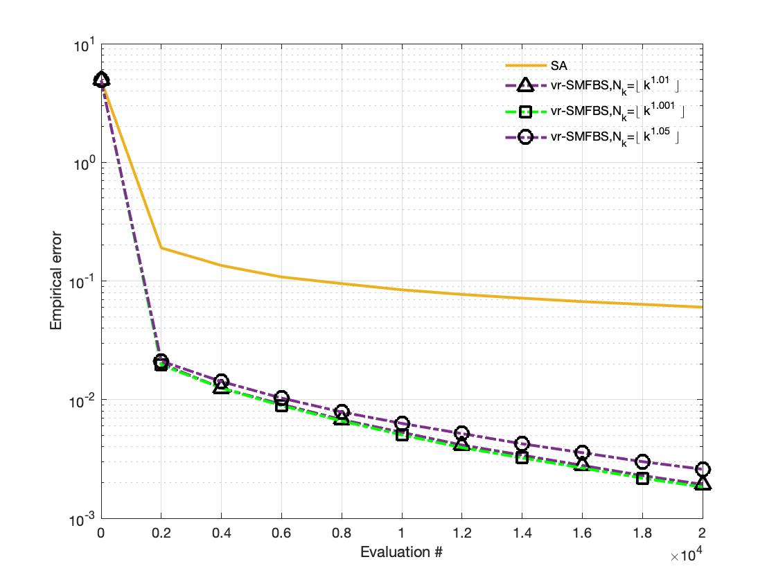
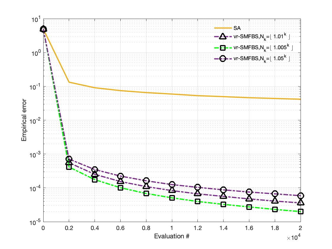
Figure 1: Trajectories for (SA) and (vr-SMBFS) (up: monotone; down: s-monotone)

We describe the three schemes being compared and specify their algorithm parameters. Solution quality is compared by estimating the residual function $\texttt{res}(x)=\|x-\Pi_{\mathcal{X}}(x-\gamma A(x))\|$.

IV-A Algorithm specifications.

(i) (SA): Stochastic approximation scheme. The (SA) scheme utilizes the following update.

$$x_{k+1}:=\Pi_{\mathcal{X}}\left[x_{k}-\gamma_{k}A(x_{k},\omega_{k})\right],$$ (SA)

where $A(x_{k})=\mathbb{E}[A(x_{k},\omega_{k})]$, and $\gamma_{k}\triangleq\tfrac{1}{\sqrt{k}}$. $x_{0}$ is randomly generated in $[0,1]^{J}$.

(ii) (vr-SMFBS): Variance-reduction stochastic modified forward-backward scheme. We choose a constant $\gamma=\tfrac{1}{4L}$ which satisfies the steplength assumption and we assume $N_{k}=\lfloor k^{1.01}\rfloor$ for merely monotone problems, $N_{k}=\lfloor 1.01^{k+1}\rfloor$ for strongly monotone problems.

IV-B Performance comparison and insights.

In Fig. 1, we compare both schemes under mere monotonicity and strong monotonicity, respectively and examine sensitivities to the sample growth rate. Standard SA schemes may struggle when the problem is ill-conditioned and we examine the performance of the schemes in such regimes and provide the results in for merely monotone and strongly monotone settings in Tables II and III, respectively.

TABLE II: Comparison of (vr-SMFBS) with (SA)

merely monotone, 20000 evaluations
$L$	vr-SMFBS			SA
	error	time	CI	error	time	CI
1e1	1.6e-3	2.6	[1.3e-3,1.8e-3]	5.3e-2	2.7	[5.0e-2,5.7e-2]
1e2	1.9e-3	2.6	[1.6e-3,2.1e-3]	6.1e-2	2.7	[5.8e-2,6.4e-2]
1e3	2.2e-3	2.6	[2.0e-3,2.5e-3]	7.6e-2	2.5	[7.3e-2,7.9e-2]
1e4	5.9e-3	2.6	[5.4e-3,6.2e-3]	9.4e-2	2.6	[9.0e-1,9.7e-1]
Complicated $\mathcal{X}$, merely monotone, 2000 evaluations
1e2	1.9e-3	6.8	[1.6e-3,2.0e-3]	6.0e-2	232	[5.7e-2,6.3e-2]

TABLE III: Comparison of (vr-SMFBS) with (SA)

strongly monotone, 20000 evaluations
$L$	vr-SMFBS			SA
	error	time	CI	error	time	CI
1e1	1.5e-5	2.6	[1.2e-5,1.7e-5]	2.9e-2	2.5	[2.7e-2,3.1e-2]
1e2	3.6e-5	2.5	[3.3e-5,3.9e-5]	4.1e-2	2.5	[3.8e-2,4.4e-2]
1e3	5.6e-5	2.5	[4.2e-6,4.7e-6]	5.5e-2	2.4	[5.2e-2,5.7e-2]
1e4	7.4e-5	2.5	[7.1e-5,7.7e-5]	6.0e-2	2.5	[5.7e-2,6.3e-2]
Complicated $\mathcal{X}$, strongly monotone, 2000 evaluations
1e3	5.6e-5	18	[4.2e-6,4.7e-6]	5.5e-2	234	[5.2e-2,5.8e-2]

Key findings. (vr-SMFBS) trajectories are characterized by significantly smaller empirical errors than (SA). There is little impact on (vr-SMFBS) when varying the sample growth rate. Moreover, (vr-SMFBS) appears to cope better with large Lipchitz constant. Since we utilize the analytical $L$ to set $\gamma$, we see smaller steps for large $L$. To show the efficiency of (vr-SMFBS) with complicated feasible set, we change $\mathcal{X}\triangleq\{x\in\mathbb{R}_{J}^{+}\mid\sum_{i}x_{i}\leq 10\}$ which leads to computationally expensive projection steps. As seen in the last row of Tables II and III, (vr-SMFBS) takes far less time than (SA).

IV-C Comparison with SAA schemes

To show the performance of our proposed schemes , we consider the (SAA) scheme used in [74]. Let $(\omega_{1i})_{i=1}^{J},(\omega_{2i})_{i=1}^{J}$, $\dots,(\omega_{\nu i})_{i=1}^{J}$ denote independent identically distributed (i.i.d.) samples. Then, with (SAA) we solve the following formulation of problem:

$$\left\{\begin{aligned} 0&\leq x_{i}\perp c_{i}^{\prime}(x_{i})+r\cdot(X+x_{i})-d+\tfrac{1}{\nu}\sum_{l=1}^{\nu}\lambda_{i}(\omega_{li})\geq 0\\ 0&\leq y_{i}(\omega_{li})\perp h_{i}(\omega_{li})+\lambda_{i}(\omega_{li})\geq 0\\ 0&\leq\lambda_{i}(\omega_{li})\perp x_{i}-y_{i}(\omega_{li})+\epsilon\lambda_{i}(\omega_{li})\geq 0,\ \forall l=1,\dots,\nu\end{aligned}\right\}$$

$$\forall i=1,\dots,J.$$

This problem is cast as a linear complementarity problem (LCP), allowing for utilizing PATH [75] to compute a solution. We compare (SAA) with (vr-SMFBS) in Table IV. From the results, we observe that although the empirical errors of both schemes are similar, the (SAA) scheme takes far longer than (vr-SMFBS) when using a large number of samples. In fact, (vr-SMFBS) scale well with overall number of evaluations.

TABLE IV: Comparison of (SAA) with (vr-SMFBS) (u: s-monotone, d: monotone)

$\nu$	SAA		vr-SMFBS
	time/s	res	time/s	res
1000	0.7	4.5e-4	0.3	4.8e-4
2000	3.3	3.5e-4	0.5	2.3e-4
4000	6.2	1.6e-4	0.6	1.0e-4
10000	32.7	3.7e-5	1.2	3.4e-5
20000	117.7	2.8e-5	2.5	1.5e-5

$\nu$	SAA		vr-SMFBS
	time/s	res	time/s	res
1000	0.7	5.6e-2	0.3	2.7e-2
2000	3.0	3.4e-2	0.5	2.0e-2
4000	5.8	2.2e-2	0.6	1.2e-2
10000	61.8	7.8e-3	1.2	5.3e-3
20000	115.0	2.5e-3	2.6	1.9e-3

V Concluding remarks

Monotone inclusions represent an important class of problems and their stochastic counterpart subsumes a large class of stochastic optimization and equilibrium problems. Such objects arise in optimization, game-theoretic, and model-predictive control problems afflicted by uncertainty. We propose a variance-reduced splitting framework for resolving such problems when the map is structured. Under suitable assumptions on the sample-size, we prove that the scheme displays a.s. convergence guarantees and achieves optimal linear and sublinear rates in strongly monotone and monotone regimes while achieving either optimal or near-optimal sample-complexities. By incorporating state-dependent bounds on noise and weakening unbiasedness requirements (in strongly monotone settubfs), we develop techniques that can accommodate far more general settings. Preliminary numerics on a class of two-stage stochastic variational inequality problems suggest that the scheme outperform stochastic approximation schemes, as well as sample-average approximation approaches.

References

- [1] S. M. Robinson, Generalized Equations, pp. 346–367. Berlin, Heidelberg: Springer Berlin Heidelberg, 1983.
- [2] R. T. Rockafellar, “Monotone operators and the proximal point algorithm,” SIAM Journal on Control and Optimization, vol. 14, no. 5, pp. 877–898, 1976.
- [3] R. Glowinski and P. Le Tallec, Augmented Lagrangian and operator-splitting methods in nonlinear mechanics, vol. 9. SIAM, 1989.
- [4] J. Douglas and H. H. Rachford, “On the numerical solution of heat conduction problems in two and three space variables,” Transactions of the American mathematical Society, vol. 82, no. 2, pp. 421–439, 1956.
- [5] D. W. Peaceman and H. H. Rachford, Jr, “The numerical solution of parabolic and elliptic differential equations,” Journal of the Society for industrial and Applied Mathematics, vol. 3, no. 1, pp. 28–41, 1955.
- [6] P.-L. Lions and B. Mercier, “Splitting algorithms for the sum of two nonlinear operators,” SIAM Journal on Numerical Analysis, vol. 16, no. 6, pp. 964–979, 1979.
- [7] G. B. Passty, “Ergodic convergence to a zero of the sum of monotone operators in Hilbert space,” Journal of Mathematical Analysis and Applications, vol. 72, no. 2, pp. 383–390, 1979.
- [8] X. Chen, A. Shapiro, and H. Sun, “Convergence analysis of sample average approximation of two-stage stochastic generalized equations,” SIAM Journal on Optimization, vol. 29, no. 1, pp. 135–161, 2019.
- [9] R. J. Aumann, “Integrals of set-valued functions,” Journal of Mathematical Analysis and Applications, vol. 12, no. 1, pp. 1–12, 1965.
- [10] G. B. Dantzig, “Linear programming under uncertainty,” in Stochastic programming, pp. 1–11, Springer, 2010.
- [11] J. R. Birge and F. Louveaux, Introduction to stochastic programming. Springer Science & Business Media, 2011.
- [12] A. Shapiro, D. Dentcheva, and A. Ruszczyński, Lectures on stochastic programming: modeling and theory. SIAM, 2014.
- [13] H. Jiang and H. Xu, “Stochastic approximation approaches to the stochastic variational inequality problem,” IEEE Transactions on Automatic Control, vol. 53, no. 6, pp. 1462–1475, 2008.
- [14] A. Juditsky, A. Nemirovski, and C. Tauvel, “Solving variational inequalities with stochastic mirror-prox algorithm,” Stochastic Systems, vol. 1, no. 1, pp. 17–58, 2011.
- [15] U. V. Shanbhag, “Stochastic variational inequality problems: Applications, analysis, and algorithms,” in Theory Driven by Influential Applications, pp. 71–107, INFORMS, 2013.
- [16] U. Ravat and U. V. Shanbhag, “On the existence of solutions to stochastic quasi-variational inequality and complementarity problems,” Mathematical Programming, vol. 165, no. 1, pp. 291–330, 2017.
- [17] U. Ravat and U. V. Shanbhag, “On the characterization of solution sets of smooth and nonsmooth convex stochastic nash games,” SIAM Journal on Optimization, vol. 21, no. 3, pp. 1168–1199, 2011.
- [18] F. Facchinei and J.-S. Pang, Finite-dimensional variational inequalities and complementarity problems. Springer Science & Business Media, 2007.
- [19] H. D. Sherali, “A multiple leader Stackelberg model and analysis,” Operations Research, vol. 32, no. 2, pp. 390–404, 1984.
- [20] J.-S. Pang and M. Fukushima, “Quasi-variational inequalities, generalized Nash equilibria, and multi-leader-follower games,” Computational Management Science, vol. 2, no. 1, pp. 21–56, 2005.
- [21] C.-L. Su, “Analysis on the forward market equilibrium model,” Operations Research Letters, vol. 35, no. 1, pp. 74–82, 2007.
- [22] A. A. Kulkarni and U. V. Shanbhag, “An existence result for hierarchical Stackelberg v/s Stackelberg games,” IEEE Transactions on Automatic Control, vol. 60, no. 12, pp. 3379–3384, 2015.
- [23] M. Herty, S. Steffensen, and A. Thünen, “Solving quadratic multi-leader-follower games by smoothing the follower’s best response,” Optimization Methods and Software, pp. 1–28, 2020.
- [24] J. B. Rawlings, D. Q. Mayne, and M. Diehl, Model predictive control: theory, computation, and design, vol. 2. Nob Hill Publishing Madison, WI, 2017.
- [25] D. A. Allan, C. N. Bates, M. J. Risbeck, and J. B. Rawlings, “On the inherent robustness of optimal and suboptimal nonlinear MPC,” Systems Control Lett., vol. 106, pp. 68–78, 2017.
- [26] A. Bemporad and M. Morari, “Robust model predictive control: A survey,” in Robustness in identification and control, pp. 207–226, Springer, 1999.
- [27] F. A. Cuzzola, J. C. Geromel, and M. Morari, “An improved approach for constrained robust model predictive control,” Automatica, vol. 38, no. 7, pp. 1183–1189, 2002.
- [28] S. Hojjatinia, C. M. Lagoa, and F. Dabbene, “Identification of switched autoregressive exogenous systems from large noisy datasets,” Internat. J. Robust Nonlinear Control, vol. 30, no. 15, pp. 5777–5801, 2020.
- [29] M. Chamanbaz, F. Dabbene, and C. M. Lagoa, “Probabilistically robust AC optimal power flow,” IEEE Trans. Control Netw. Syst., vol. 6, no. 3, pp. 1135–1147, 2019.
- [30] C. Feng, F. Dabbene, and C. M. Lagoa, “A kinship function approach to robust and probabilistic optimization under polynomial uncertainty,” IEEE Trans. Automat. Control, vol. 56, no. 7, pp. 1509–1523, 2011.
- [31] A. Ben-Tal, L. El Ghaoui, and A. Nemirovski, Robust optimization. Princeton university press, 2009.
- [32] P. K. Mishra, S. S. Diwale, C. N. Jones, and D. Chatterjee, “Reference tracking stochastic model predictive control over unreliable channels and bounded control actions,” Automatica J. IFAC, vol. 127, pp. 109512, 10, 2021.
- [33] J. Zhang and T. Ohtsuka, “Stochastic model predictive control using simplified affine disturbance feedback for chance-constrained systems,” IEEE Control Syst. Lett., vol. 5, no. 5, pp. 1633–1638, 2021.
- [34] Y. Tan, Q. Cao, L. Li, T. Hu, and M. Su, “A chance-constrained stochastic model predictive control problem with disturbance feedback,” J. Ind. Manag. Optim., vol. 17, no. 1, pp. 67–79, 2021.
- [35] L. Hewing and M. N. Zeilinger, “Scenario-based probabilistic reachable sets for recursively feasible stochastic model predictive control,” IEEE Control Syst. Lett., vol. 4, no. 2, pp. 450–455, 2020.
- [36] A. Groß, C. Wittwer, and M. Diehl, “Stochastic model predictive control of photovoltaic battery systems using a probabilistic forecast model,” Eur. J. Control, vol. 56, pp. 254–264, 2020.
- [37] L. Hewing, K. P. Wabersich, and M. N. Zeilinger, “Recursively feasible stochastic model predictive control using indirect feedback,” Automatica J. IFAC, vol. 119, pp. 109095, 7, 2020.
- [38] A. Mesbah, “Stochastic model predictive control: An overview and perspectives for future research,” IEEE Control Systems Magazine, vol. 36, no. 6, pp. 30–44, 2016.
- [39] E. Camacho and C. Alba, Model Predictive Control. Advanced Textbooks in Control and Signal Processing, Springer London, 2013.
- [40] I. E. Bardakci, A. Jalilzadeh, C. Lagoa, and U. V. Shanbhag, “Probability maximization via minkowski functionals: Convex representations and tractable resolution,” arXiv preprint arXiv:1802.09682, 2018.
- [41] L. Rosasco, S. Villa, and B. C. Vũ, “Stochastic forward–backward splitting for monotone inclusions,” Journal of Optimization Theory and Applications, vol. 169, no. 2, pp. 388–406, 2016.
- [42] P. L. Combettes and J.-C. Pesquet, “Stochastic approximations and perturbations in forward-backward splitting for monotone operators,” Pure and Applied Functional Analysis, vol. 1, no. 1, pp. 13–37, 2016.
- [43] A. Ruszczyński, “Decomposition methods in stochastic programming,” Mathematical Programming, vol. 79, no. 1-3, pp. 333–353, 1997.
- [44] M. Schmidt, N. L. Roux, and F. R. Bach, “Convergence rates of inexact proximal-gradient methods for convex optimization,” in Advances in neural information processing systems, pp. 1458–1466, 2011.
- [45] S. Ghadimi, G. Lan, and H. Zhang, “Mini-batch stochastic approximation methods for nonconvex stochastic composite optimization,” Mathematical Programming, vol. 155, no. 1-2, Ser. A, pp. 267–305, 2016.
- [46] A. Jalilzadeh, U. V. Shanbhag, J. H. Blanchet, and P. W. Glynn, “Smoothed variable sample-size accelerated proximal methods for nonsmooth stochastic convex programs,” arXiv preprint arXiv:1803.00718, 2018.
- [47] A. Jofré and P. Thompson, “On variance reduction for stochastic smooth convex optimization with multiplicative noise,” Mathematical Programming, vol. 174, no. 1-2, pp. 253–292, 2019.
- [48] L. Rosasco, S. Villa, and B. C. Vũ, “Convergence of stochastic proximal gradient algorithm,” Applied Mathematics & Optimization, pp. 1–27, 2019.
- [49] S. Cui and U. V. Shanbhag, “On the analysis of reflected gradient and splitting methods for monotone stochastic variational inequality problems,” in 55th IEEE Conference on Decision and Control, CDC 2016, Las Vegas, NV, USA, December 12-14, 2016, pp. 4510–4515, IEEE, 2016.
- [50] V. G. Yaji and S. Bhatnagar, “Analysis of stochastic approximation schemes with set-valued maps in the absence of a stability guarantee and their stabilization,” IEEE Trans. Autom. Control., vol. 65, no. 3, pp. 1100–1115, 2020.
- [51] V. G. Yaji and S. Bhatnagar, “Stochastic recursive inclusions in two timescales with nonadditive iterate-dependent markov noise,” Math. Oper. Res., vol. 45, no. 4, pp. 1405–1444, 2020.
- [52] V. Cevher, B. C. Vũ, and A. Yurtsever, “Stochastic forward Douglas-Rachford splitting method for monotone inclusions,” in Large-Scale and Distributed Optimization, pp. 149–179, Springer, 2018.
- [53] X. Chen, R. J.-B. Wets, and Y. Zhang, “Stochastic variational inequalities: residual minimization smoothing sample average approximations,” SIAM Journal on Optimization, vol. 22, no. 2, pp. 649–673, 2012.
- [54] A. Shapiro and H. Xu, “Stochastic mathematical programs with equilibrium constraints, modelling and sample average approximation,” Optimization, vol. 57, no. 3, pp. 395–418, 2008.
- [55] M. P. Friedlander and M. Schmidt, “Hybrid deterministic-stochastic methods for data fitting,” SIAM Journal on Scientific Computing, vol. 34, no. 3, pp. A1380–A1405, 2012.
- [56] R. H. Byrd, G. M. Chin, J. Nocedal, and Y. Wu, “Sample size selection in optimization methods for machine learning,” Mathematical Programming, vol. 134, no. 1, pp. 127–155, 2012.
- [57] R. Pasupathy, P. Glynn, S. Ghosh, and F. S. Hashemi, “On sampling rates in simulation-based recursions,” SIAM Journal on Optimization, vol. 28, no. 1, pp. 45–73, 2018.
- [58] S. Ghadimi, G. Lan, and H. Zhang, “Mini-batch stochastic approximation methods for nonconvex stochastic composite optimization,” Mathematical Programming, vol. 155, no. 1-2, pp. 267–305, 2016.
- [59] R. Bollapragada, D. Mudigere, J. Nocedal, H. M. Shi, and P. T. P. Tang, “A progressive batching L-BFGS method for machine learning,” in Proceedings of the 35th International Conference on Machine Learning, ICML 2018, Stockholmsmässan, Stockholm, Sweden, July 10-15, 2018 (J. G. Dy and A. Krause, eds.), vol. 80 of Proceedings of Machine Learning Research, pp. 619–628, PMLR, 2018.
- [60] A. Jalilzadeh, A. Nedic, U. V. Shanbhag, and F. Yousefian, “A variable sample-size stochastic quasi-newton method for smooth and nonsmooth stochastic convex optimization,” Mathematics of Operations Research (to appear), https://arxiv.org/abs/1804.05368, 2020.
- [61] R. Johnson and T. Zhang, “Accelerating stochastic gradient descent using predictive variance reduction,” in Advances in Neural Information Processing Systems (C. J. C. Burges, L. Bottou, M. Welling, Z. Ghahramani, and K. Q. Weinberger, eds.), vol. 26, pp. 315–323, Curran Associates, Inc., 2013.
- [62] A. Defazio, F. Bach, and S. Lacoste-Julien, “SAGA: A fast incremental gradient method with support for non-strongly convex composite objectives,” in Advances in Neural Information Processing Systems (Z. Ghahramani, M. Welling, C. Cortes, N. Lawrence, and K. Q. Weinberger, eds.), vol. 27, pp. 1646–1654, Curran Associates, Inc., 2014.
- [63] S.-P. Han and G. Lou, “A parallel algorithm for a class of convex programs,” SIAM Journal on Control and Optimization, vol. 26, no. 2, pp. 345–355, 1988.
- [64] P. Tseng, “A modified forward-backward splitting method for maximal monotone mappings,” SIAM Journal on Control and Optimization, vol. 38, no. 2, pp. 431–446, 2000.
- [65] B. T. Polyak, Introduction to optimization. Optimization Software New York, 1987.
- [66] T. Larsson and M. Patriksson, “A class of gap functions for variational inequalities,” Mathematical Programming, vol. 64, no. 1, Ser. A, pp. 53–79, 1994.
- [67] J. M. Borwein and J. Dutta, “Maximal monotone inclusions and Fitzpatrick functions,” Journal of Optimization Theory and Applications, vol. 171, no. 3, pp. 757–784, 2016.
- [68] J. M. Borwein and J. D. Vanderwerff, Convex functions: constructions, characterizations and counterexamples, vol. 109. Cambridge University Press Cambridge, 2010.
- [69] S. Fitzpatrick, “Representing monotone operators by convex functions,” in Workshop/Miniconference on Functional Analysis and Optimization, pp. 59–65, Centre for Mathematics and its Applications, Mathematical Sciences Institute, The Australian National University, 1988.
- [70] Y. Nesterov, “Dual extrapolation and its applications to solving variational inequalities and related problems,” Mathematical Programming, vol. 109, no. 2, pp. 319–344, 2007.
- [71] A. Iusem, A. Jofré, R. I. Oliveira, and P. Thompson, “Extragradient method with variance reduction for stochastic variational inequalities,” SIAM Journal on Optimization, vol. 27, no. 2, pp. 686–724, 2017.
- [72] R. Bot, P. Mertikopoulos, M. Staudigl, and P. Vuong, “Mini-batch forward-backward-forward methods for solving stochastic variational inequalities,” Stochastic Systems, 2020.
- [73] H. Ahmadi, On the analysis of data-driven and distributed algorithms for convex optimization problems. The Pennsylvania State University, 2016.
- [74] J. Jiang, Y. Shi, X. Wang, and X. Chen, “Regularized two-stage stochastic variational inequalities for cournot-nash equilibrium under uncertainty,” arXiv preprint arXiv:1907.07317, 2019.
- [75] S. P. Dirkse and M. C. Ferris, “The path solver: a nommonotone stabilization scheme for mixed complementarity problems,” Optimization Methods and Software, vol. 5, no. 2, pp. 123–156, 1995.