Quaternion-Based Self-Attentive Long Short-term User Preference Encoding for Recommendation

Abstract.

Quaternion space has brought several benefits over the traditional Euclidean space: Quaternions (i) consist of a real and three imaginary components, encouraging richer representations; (ii) utilize Hamilton product which better encodes the inter-latent interactions across multiple Quaternion components; and (iii) result in a model with smaller degrees of freedom and less prone to overfitting. Unfortunately, most of the current recommender systems rely on real-valued representations in Euclidean space to model either user’s long-term or short-term interests. In this paper, we fully utilize Quaternion space to model both user’s long-term and short-term preferences. We first propose a QUaternion-based self-Attentive Long term user Encoding (QUALE) to study the user’s long-term intents. Then, we propose a QUaternion-based self-Attentive Short term user Encoding (QUASE) to learn the user’s short-term interests. To enhance our models’ capability, we propose to fuse QUALE and QUASE into one model, namely QUALSE, by using a Quaternion-based gating mechanism. We further develop Quaternion-based Adversarial learning along with the Bayesian Personalized Ranking (QABPR) to improve our model’s robustness. Extensive experiments on six real-world datasets show that our fused QUALSE model outperformed 11 state-of-the-art baselines, improving 8.43% at HIT@1 and 10.27% at NDCG@1 on average compared with the best baseline.

1. Introduction

Recommender Systems (Resnick and Varian, 1997) have become the heart of many online applications such as e-commerce, music/video streaming services, social media, etc. Recommender systems proactively helped (i) users to explore new/unseen items, (ii) potentially the users stay longer on the applications, and (iii) companies increase their revenue.

Matrix Factorization techniques (Koren et al., 2009; Hu et al., 2008; He et al., 2016) extracted features of users and items to compute their similarity. Recently, deep neural network boosted performance of a recommender system by providing non-linearity which helped modeling complex relationships between users and items (He et al., 2017b). However, these prior works only focused on a user and a target item without considering the user’s previously consumed items, some of which may be related to the target item. While some prior works (Koren, 2008; Kabbur et al., 2013) largely premised on unordered user interactions, users’ interests are intrinsically dynamic and evolving. Based on the observation, (He et al., 2017a; Rendle et al., 2010; Tang and Wang, 2018; Kang and McAuley, 2018; Hidasi et al., 2016) followed two paradigms to capture a user’s sequential pattern: (i) short-term item-item transitions, or (ii) long-term item-item transitions.

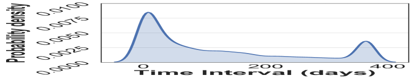
(a) Video Games

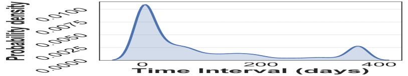
(b) Toys and Games

Figure 1. Density distribution of item-item similarity scores on Amazon Video Games, and Toys and Games datasets.

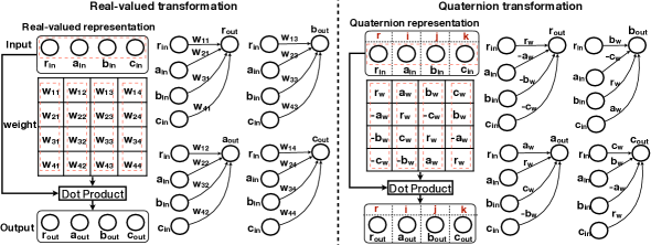
Figure 2. Comparison between real-valued transformation (Left) and Quaternion transformation (Right). We replace Hamilton product in Quaternion space with an equivalent dot product in real space for an easy reference.

However, user’s interests can be highly diverse, so modeling only either short-term or long-term user intent does not fully capture the user’s preferences, producing less effective recommendation results. To illustrate the point, we conducted an empirical analysis on Amazon Video Games, and Toys and Games datasets. First, we represent each item by a multi-hot encoding, where item $j$ is represented by a vector $t\in\mathbb{R}^{m}$, position $i=1$ if user $i$ consumed the current item, and $m$ denotes the total number of users in a dataset. For each user, her consumed items are sorted in the chronological order. Then, we calculated a cosine similarity score between each item and each of its previously consumed items. Then we selected the largest cosine similarity score per item per user. Figure 1 presents the density distribution of the consumed time interval (x-axis) between each pair of item and its most similar previously consumed item. We observe that there exists a bimodal distribution, where one (left) peak lays at a relative short-term period and the other (right) peak locates in a long-term period. The observation confirms that both long-term and short-term preferences played important roles on the user’s current purchasing intent. We observe the same phenomenon from the other four datasets described in Section 6.

Based on the observation, we propose a Quaternion-based neural recommender system that models both long-term and short-term user preferences. Unlike the prior works (Zhou et al., 2019; Yu et al., 2019) which rely on Euclidean space, our proposed recommender system models both user’s long-term and short-term preferences in a hypercomplex system (i.e., Quaternion Space) to further improve the recommendation quality. Concretely, we utilize Quaternion representations for all users, items and neural transformations in our proposed models. There are numerous benefits of the Quaternion utilization over the traditional real-valued representations in Euclidean space: (1) Quaternion numbers/vectors consist of a real component and three imaginary components (i.e. $\bm{i,j,k}$), encouraging a richer extent of expressiveness; (2) instead of using dot product in Euclidean space, Quaternion numbers/vectors operate on Hamilton product, which matches across multiple (inter-latent) Quaternion components and strengthens their inter-latent interactions, leading to a higher expressive model; (3) the weight sharing nature of Hamilton product leads to a model with a smaller number of parameters.

To illustrate these benefits of the Quaternion utilization, we show a comparison of a transformation process with Quaternion representations vs. real-valued representations in Figure 2. In Euclidean space, different output dimensions are produced by multiplying the same input with different weights. Given a real-valued 4-dimensional vector $[r_{in},a_{in},b_{in},c_{in}]$, it takes a total of 16 parameters (i.e. 16 degrees of freedom) to transform into $[r_{out},a_{out},b_{out},$ $c_{out}]$. For Quaternion transformation, the input vector now is represented with 4 components, where $r_{in}$ is the value of the real component, $a_{in}$, $b_{in}$, $c_{in}$ are the corresponding values of the three imaginary parts $\bm{i}$, $\bm{j}$, $\bm{k}$. Due to the weight sharing nature of Hamilton product (refer to the Equa (3) in Section 4), different output dimensions take different combinations of the same input with only 4 weighting parameters {$r_{w},a_{w},b_{w},c_{w}$}. The Quaternions provide a better inter-dependencies interaction coding and reduce 75% of the number of parameters compared with real-valued representations in Euclidean space (e.g., 4 unique parameters vs. 16 parameters).

To our best of knowledge, we are the first work that fully utilizes Quaternion space in modeling both user’s long-term and short term interests. Furthermore, to increase our model’s robustness, we propose a Quaternion-based Adversarial attack on Bayesian Personalized Ranking (QABPR) loss. As far as we know, we are the first, applying adversarial attack on Quaternion representations in the recommendation domain.

We summarize our contributions in the paper as follows:

• We propose novel Quaternion based models to learn a user’s long-term and short-term interests more effectively. As a part of our framework, we propose Quaternion self-attention that works in Quaternion space.

• We propose a Quaternion-based Adversarial attack on BPR-loss to further improve the robustness of our model.

• We conduct extensive experiments to demonstrate the effectiveness of our models against 11 strong state-of-the-art baselines on six real-world datasets.

2. Related Work

General Recommenders. Matrix Factorization is the most popular method to encode global user representations by using unordered user-item interactions (Hu et al., 2008; Koren et al., 2009; Zhang et al., 2016). Its basic idea is to represent users and items by latent factors and use dot product to learn the user-item affinity. Despite their success, they cannot model non-linear user-item relationships due to the linear nature of dot product. To overcome the limitation, neural network based recommenders were recently introduced (He et al., 2017b; Vinh Tran et al., 2019; Tran et al., 2019b; Ebesu et al., 2018). (He et al., 2017b) combined a generalized matrix factorization component and a non-linear user-item interactions via a MLP architecture. (Ma et al., 2018; Liang et al., 2018; Ma et al., 2019b) substituted the MLP architecture with the auto-encoder design. (Xin et al., 2019; Tran et al., 2019a) used memory augmentation to learn different user-item latent relationship. When non-existed users come with some observed interactions (i.e., recently created user accounts with some item interactions), the recommenders need to be rebuilt to generate their representations. To avoid these issues, current works encode users by combining the users’ consumed item embeddings in two main streams: (i) taking average of the consumed items’ latent representations (Koren, 2008; Kabbur et al., 2013), or (ii) attentively summing (He et al., 2018b) the consumed items’ embeddings.

Despite their success, general recommenders mostly consider all users’ unordered consumed items, and produce global/long-term user representations, which are supposed to be static, or changed slowly. Thus, they failed to capture the user’s dynamic behavior, that is captured by the user’s short-term preference (see Figure 1).

Sequential Recommenders. Sequential recommendation is known for its superiority to capture temporal dependencies between historical items (Ma et al., 2019a). Early works relied on Markov Chains to capture item-item sequential patterns (Feng et al., 2015; Rendle et al., 2010; He et al., 2017a). Other works exploited the convolution architecture to capture more complex temporal dependencies (Tang and Wang, 2018). These methods used short-term item dependencies to model a user’s dynamic interest. Other sequential recommenders focused on modeling long-term user preferences using RNN-based architectures (Hidasi et al., 2016; Wu et al., 2017; Li et al., 2017; Liu et al., 2016). However, modeling either long-term user interests or short-term user interests is suboptimal since they concurrently affect a user’s intent (Figure 1). Recent works combined both long and short-term user preferences in real-valued representations to obtain satisfactory results (Kang and McAuley, 2018; Zhou et al., 2019; Yu et al., 2019).

Compared with the prior works which used real-valued representations , we propose Quaternion-based models to capture the user’s long-term and short-term interests. Quaternion was first introduced by (Hamilton, 1844) and it has recently shown its effectiveness over real-valued representations in NLP and computer vision domains (Zhu et al., 2018; Gaudet and Maida, 2018; Parcollet et al., 2019a; Tay et al., 2019). We acknowledge that QCF model (Zhang et al., 2019) is the first Quaternion-based recommender. However, the authors used it as a simple extension of the matrix factorization method, where users and items are Quaternion embeddings. Thus, the benefits of Quaternion representation were not fully exploited in their network. Furthermore, they designed the model for a general recommendation problem, which has an inherent limitation of only modeling the user’s global interest.

3. Problem Definition

Denote U={$u_{1},u_{2},...,u_{m}$} as a set of all users where $m=|U|$ is the total number of users, and P={$p_{1},p_{2},...,p_{n}$} as a set of all items where $n=|P|$ is the total number of items. Bold versions of those variables, which we will introduce in the following sections, indicate their respective latent representations/embeddings. Each user $u_{i}\in U$ consumes items in $P$, denoted by a chronological list $T^{(u_{i})}$. We denote $L^{(u_{i})}$ as the chronological list of long-term consumed items of $u_{i}$, and $S^{(u_{i})}$ as the chronological list of short-term consumed items of $u_{i}$ (i.e. $s$ most recently consumed items in chronological order of the user $u_{i}$), $L^{u_{i}}\cup S^{u_{i}}=T^{(u_{i})}$. Note that bold versions of $\bm{i},\bm{j},\bm{k}$ are used to indicate the three imaginary parts of a Quaternion, while their subscript versions are used as indices.

In this work, we propose and build Quaternion-based recommender systems by using both long-term and short-term user interests, denoted as $P(p_{j}|L^{(u_{i})},S^{(u_{i})})$. Under an assumption that $L^{(u_{i})}$ and $S^{(u_{i})}$ are independent given the target item $p_{j}$, we model $P(p_{j}|L^{(u_{i})},S^{(u_{i})})$ by modeling the user’s long-term interest $P(p_{j}|L^{(u_{i})})$ and short-term interest $P(p_{j}|S^{(u_{i})})$ separately by using two different Quaternion-based neural networks. Then, we automatically fuse the two models to build a more effective recommender system.

4. Preliminary on Quaternion

In this section, we cover important background on Quaternion Algebra and Quaternion Operators that we use to design our models.

Quaternion number: In mathematics, Quaternions are a hypercomplex number system. A Quaternion number X in a Quaternion space $\mathbb{H}$ is formed by a real component (r) and three imaginary components as follows:

(1) $$X=r+a\bm{i}+b\bm{j}+c\bm{k},$$

where $\bm{ijk}=\bm{i^{2}}=\bm{j^{2}}=\bm{k^{2}}=-1$. The non-commutative multiplication rules of quaternion numbers are: $\bm{ij}=\bm{k}$, $\bm{jk}=\bm{i}$, $\bm{ki}=\bm{j}$, $\bm{ji}=-\bm{k}$, $\bm{kj}=-\bm{i}$, $\bm{ik}=-\bm{j}$. In Equa (1), $r,a,b,c$ are real numbers $\in\mathbb{R}$. Note that we can extend $r,a,b,c$ to real-valued vectors to obtain a Quaternion embedding, which we use to represent each user/item’s latent features and conduct neural transformations. Operations on Quaternion embeddings are similar to Quaternion numbers.

Component-wise Quaternion Operators: Let $f$ define an algebraic operator in real space $\mathbb{R}$. The component-wise Quaternion operator $f$ on two Quaternions $X,Y\in\mathbb{H}$ is defined as:

(2) $$f(X,Y)=f(r_{X},r_{Y})+f(a_{X},a_{Y})\bm{i}+f(b_{X},b_{Y})\bm{j}+f(c_{X},c_{Y})\bm{k}$$

For instance, if $f$ is an addition operator (i.e. $f(a,b)=a+b$), then $f(X,Y)$ returns a component-wise Quaternion addition between $X$ and $Y$. If $f$ is a dot product operator (i.e. $f(a,b)=a^{T}b$), then $f(X,Y)$ returns a component-wise Quaternion dot product between $X$ and $Y$. A similar description is applied when $f$ is either subtraction, scalar multiplication, product, softmax, or concatenate operator, .etc.

Hamilton Product: The Hamilton product (denoted by the $\otimes$ symbol) of two Quaternions $X\in\mathbb{H}$ and $Y\in\mathbb{H}$ is defined as:

(3) $$X\otimes Y= (r_{X}r_{Y}-a_{X}a_{Y}-b_{X}b_{Y}-c_{X}c_{Y})\;+$$

$$(r_{X}a_{Y}+a_{X}r_{Y}+b_{X}c_{Y}-c_{X}b_{Y})\bm{i}\;+$$

$$(r_{x}b_{Y}-a_{X}c_{Y}+b_{X}r_{Y}+c_{X}a_{Y})\bm{j}\;+$$

$$(r_{X}c_{Y}+a_{X}b_{Y}-b_{X}a_{Y}+c_{X}r_{Y})\bm{k}$$

Activation function on Quaternions: Similar to (Parcollet et al., 2019b; Gaudet and Maida, 2018), we use a split activation function because of its stability and simplicity. Split activation function $\beta$ on a Quaternion $X$ is defined as:

(4) $$\beta(X)=\alpha(r)+\alpha(a)\bm{i}+\alpha(b)\bm{j}+\alpha(c)\bm{k}$$

, where $\alpha$ is any standard activation function for real values.

Concatenate four components of a Quaternion: concatenates all four Quaternion components into one real-valued vector:

(5) $$=[r_{X},a_{X},b_{X},c_{X}]$$

5. Our proposed models

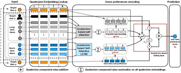
Figure 3. Our proposed architecture for modeling both long and short-term user interests using Quaternion representations.

Figure 3 shows an overview of our proposals. First, our QUaternion-based self-Attentive Long term user Encoding (QUALE) learns a user’s long-term interest by using long-term consumed items and the target item. Second, our QUaternion-based self-Attentive Short term user Encoding (QUASE) encodes the user’s short-term intent by using short-term consumed items and the target item. Then our QUaternion-based self-Attentive Long Short term user Encoding (QUALSE) fuses both of the user preferences by using a Quaternion-based gating layer. We describe each component as follows:

5.1. QUaternion-based self-Attentive Long term user encoding (our QUALE model)

The most widely used technique for modeling the user long-term interests is the Asymmetric-SVD (ASVD) (Koren, 2008) model. Its basic idea is to encode each user and item by latent representations where the user representation is encoded by summing latent representations of the user’s interacted items. To an extent, we propose a QUaternion-based self-Attentive Long term user Encoding (QUALE). QUALE represents each user and each item as Quaternion embeddings. Then, we encode each user by attentively summing Quaternion embeddings of her interacted items as follows:

(6) $$\bm{u_{i}}^{(long)}=\sum^{|L^{(u_{i})}|}_{k=1}\alpha_{k}\times\bm{p_{k}}^{(long)}\vspace{-2pt}$$

where $\bm{u_{i}}^{(long)},\bm{p_{k}}^{(long)}\in\mathbb{H}$. The summation “$\sum$” and the multiplication “$\times$” are Quaternion component-wise operators, which are calculated by using Equa (2). We use our proposed Quaternion personalized self-attention mechanism to assign attentive scores $\alpha_{k}\in\mathbb{H}$ for different long-term items $p_{k}$.

Our QUALE model has four layers: Input, Quaternion Embedding, Encoding, and Output layers. We detail each layer as follows:

5.1.1. Input

QUALE requires a target user $u_{i}$, a target item $p_{j}$, and the user’s list of $l$ long-term items $L^{(u_{i})}$ with $|L^{(u_{i})}|=l$. $l$ could be simply set to the maximum number of long-term items among all the users in a dataset. However, we observed that only several users in our datasets consumed an extremely large number of items compared to the majority of users. Hence, we set $l$ to the upper bound of the boxplot approach (i.e. Q3 + 1.5IQR, where Q3 is the third quartile, and IQR is the Interquartile range of the sequence length distribution of all users). If a user has consumed less than $l$ items, we pad the list with zeroes until its length reaches $l$.

5.1.2. Quaternion Embedding layer

It holds two Quaternion embedding matrices: a user context Quaternion embedding matrix $\mathcal{U}^{(long)}\in\mathbb{H}^{m\times d}$, and an item Quaternion embedding matrix $\mathcal{P}^{(long)}$ $\in$ $\mathbb{H}^{n\times d}$. Here, $m$ and $n$ are the respective number of users and items in the system. $d$ is the Quaternion embedding size, and is measured by the total size of real-valued vectors of four Quaternion components ($d=|r|+|a|+|b|+|c|$, and $|r|=|a|=|b|=|c|=d/4$). By passing the target user $u_{i}$, the target item $p_{j}$, and long-term items $p_{k}$ in the Input layer through the two respective Quaternion embedding matrices, we obtain the corresponding user context Quaternion embedding $\bm{q_{i}}^{(long)}$, target item Quaternion embedding $\bm{p_{j}}^{(long)}$ and long-term item Quaternion embeddings $\bm{p_{k}}^{(long)}$.

5.1.3. Encoding layer

Its main goal is to compute attentive scores for $l$ Quaternion item embeddings in Equa (6). To do so, we propose a Quaternion personalized self-attention mechanism as follows:

We first compute the Hamilton product between each long-term item Quaternion embedding $\bm{p_{k}}^{(long)}$ ($k=\overline{1,l}$) and the Quaternion context embedding $\bm{q_{i}}^{(long)}$ of the target user $u_{i}$. Next, we use Equa (2) to multiply the results with the scaling factor $1/\sqrt{d}$ to eliminate the scaling effects. Then, we apply Component-wise Softmax (Equa (2)) to obtain Quaternion attention scores as follows:

(7)

.

To obtain the attentive long-term user encoding $\bm{u_{i}}^{(long)}$ of the user $u_{i}$, we first perform the component-wise product between the attention scores $[\alpha_{1},\alpha_{2},...,\alpha_{l}]$ obtained in Equa (7) with its corresponding item Quaternion embeddings $[p_{1}^{(long)},p_{2}^{(long)},$ $...,p_{l}^{(long)}]$. Then we sum them up to obtain $\bm{u_{i}}^{(long)}$ as follows:

(8) $$\bm{u_{i}}^{(long)}=\sum_{k=1}^{l}\alpha_{k}\times\bm{p_{k}}^{(long)}\vspace{-2pt}$$

Our proposed Quaternion personalized self-attention mechanism vs. the existing self-attention mechanism: Our proposed Quaternion personalized self-attention mechanism is different from the self-attention mechanism that has been widely used in the NLP tasks in two aspects. First, unlike the prior work (Zhong et al., 2018), which uses a single global context to assign attentive scores for different dialogue states, our attention mechanism provides personalized contexts for different users. In the recommendation domain, the long-term/general user interests are supposed to be changed slowly, but user interests are various across users. In other words, a user’s long-term context is quite static, but different from another user. Hence, using personalized contexts for different users is better than using a single global context, which is not personalized. Second, our attention mechanism adopts Hamilton product and works for Quaternion embeddings as input, instead of the real-valued embeddings like traditional self-attention mechanisms.

5.1.4. Output

We produce a long-term preference score $o^{(long)}_{ij}$ between the target user $u_{i}$ and the target item $p_{j}$ by computing the Component-wise dot product between the user long-term Quaternion encoding $\bm{u_{i}}^{(long)}$ obtained in Equa (8) and the target item Quaternion embedding $\bm{p_{j}}^{(long)}$. This results in a Quaternion score . To obtain a real-valued scalar preference score used in the parameter estimation phase, we compute the average of the scalar values of four Quaternion components by following (Zhang et al., 2019):

(9) $$o^{(\text{long})}_{ij}=\text{Average}(\text{ComponentDot}(\bm{u_{i}}^{(long)},\bm{p_{j}}^{(long)}))$$

5.2. QUaternion-based self-Attentive Short term user Encoding (our QUASE model)

RNN-based models have gained a lot of attention because of their capability to capture item-to-item relationships (Zhou et al., 2019; Wu et al., 2017; Okura et al., 2017). However, due to its limitation in modeling a long sequence, we only exploit the RNN architecture to encode a user’s short-term interest. Recently, (Parcollet et al., 2019b) has introduced a Quaternion LSTM (QLSTM) model and has shown its efficiency and effectiveness over a traditional real-valued LSTM model. However, QLSTM used only the last hidden state as a latent summary of the input, which is suboptimal. To an extent, we propose a Quaternion-based self-Attentive LSTM model to learn a user’s short-term interest. We name our proposal as a QUaternion-based self-Attentive Short term user Encoding (QUASE). QUASE has 4 layers: Input, Quaternion Embedding, Encoding, and Output layers. We describe each layer as follows:

5.2.1. Input

A target item $p_{j}$, and the chronological list of $s$ short-term consumed items $S^{(u_{i})}$ of the target user $u_{i}$ with $|S^{(u_{i})}|=s$, where $s$ represents the maximum number of short-term items among all the users in a dataset. If a user has consumed less than $s$ items, we pad the list with zeroes until its length reaches $s$.

5.2.2. Quaternion Embedding layer

It holds an item Quaternion Embedding matrix $\mathcal{P}^{(short)}$ $\in\mathbb{H}^{n\times d}$. By passing the target item $p_{j}$, and $s$ short-term items in the $S^{(u_{i})}$ of the target user $u_{i}$ through $P^{short}$, we obtain their corresponding Quaternion embeddings $\bm{p_{j}}^{(short)}$, and {$\bm{p_{1}}^{(short)},\bm{p_{2}}^{(short)},...,\bm{p_{s}}^{(short)}$}.

5.2.3. Encoding layer

In this layer, we adapt the recently introduced Quaternion-based LSTM to model the item-item sequential transition. Denote $\bm{p_{t}^{(short)}}$ is the Quaternion embedding of the $t^{th}$ short-term item $p_{t}\in S^{(u_{i})}$ ($t=\overline{1,s}$). Let $f_{t},i_{t},o_{t},c_{t}$, and $h_{t}$ be the forget gate, input gate, output gate, cell state, and the hidden state of a Quaternion LSTM cell at time step $t$, respectively. We compute these variables as follows:

(10) $$f_{t} =\sigma(W_{f}\otimes\bm{p_{t}}^{(short)}+R_{f}\otimes\bm{h_{t-1}}+g_{f})$$

$$i_{t} =\sigma(W_{i}\otimes\bm{p_{t}}^{(short)}+R_{i}\otimes\bm{h_{t-1}}+g_{i})$$

$$o_{t} =\sigma(W_{o}\otimes\bm{p_{t}}^{(short)}+R_{o}\otimes\bm{h_{t-1}}+g_{o})$$

$$c_{t} =f_{t}\times c_{t-1}+i_{t}\times\text{tanh}(W_{c}\otimes\bm{p_{t}}^{(short)}+R_{c}\otimes\bm{h_{t-1}}+g_{c})$$

$$h_{t} =o_{t}\times tanh(c_{t})$$

, where $W_{f},R_{f},W_{i},R_{i},W_{o},R_{o},W_{c},R_{c}$ are Quaternion weight matrices. $g_{f},g_{i},g_{o},g_{c}$ are Quaternion bias vectors. $f_{t},i_{t},o_{t},c_{t},h_{t}$ are Quaternion vectors. The “$\times$” sign denotes a component-wise product operator, which is calculated using Equa (2). sigmoid $\sigma$ and tanh are split activation functions and are computed using the Equa (4).

Using Equa (10), given $s$ short-term consumed items $p_{1},p_{2},...,p_{s}$, we obtain their respective output Quaternion hidden states $\bm{h_{1}},\bm{h_{2}},$ $...,\bm{h_{s}}$. Then, we propose a Quaternion self-attention mechanism to combine all $s$ output Quaternion hidden states before using it to predict the next item. Different from the long-term user preferences where they are supposed to be static or changed very slowly, the short-term user interests are dynamic and changed quickly. Hence, using a static user context for each user to make personalized attention like what we did for the QUALE model is not ideal. Instead, we define a Quaternion global context vector to capture the sequential transition patterns from item to item among all the users. Denote $q$ as a Quaternion global context vector, the Quaternion-based self-attention score of each hidden state $h_{t}$ is measured by:

(11) $$\begin{bmatrix}\alpha_{1}^{(short)}\\ \alpha_{2}^{(short)}\\ \dots\\ \alpha_{s}^{(short)}\\ \end{bmatrix}=\text{ComponentSoftmax}\begin{pmatrix}\begin{bmatrix}{\bm{h_{1}}\otimes\bm{q}}/{\sqrt{d}}\\ {\bm{h_{2}}\otimes\bm{q}}/{\sqrt{d}}\\ \dots\\ {\bm{h_{t}}\otimes\bm{q}}/{\sqrt{d}}\\ \end{bmatrix}\end{pmatrix}$$

, where $\alpha_{1}^{(short)},\alpha_{2}^{(short)},...,\alpha_{s}^{(short)}$ are Quaternion numbers. To achieve the final short-term user Quaternion encoding, we perform a component-wise product between the Quaternion hidden states and their respective Quaternion attention scores, followed by a Hamilton product with a Quaternion weight matrix $W$ and the split activation function tanh:

(12) $$\bm{u_{i}}^{(short)}=tanh\bigg{(}W\otimes\bigg{(}\sum_{t=1}^{s}\alpha_{t}^{(short)}\times\bm{h_{t}}\bigg{)}\bigg{)}\vspace{-2pt}$$

Note that we also designed a Quaternion self-Attentive GRU , but its performance was slightly worse than the Quaternion self-Attentive LSTM (see Table 2 in Section 6). Thus, we only described the Quaternion self-Attentive LSTM due to space limitation.

5.2.4. Output

Similar to Equa (9), we produce the user $u_{i}$ short-term preference score $o_{ij}^{(short)}$ over the target item $p_{j}$ as follows:

(13) $$o_{ij}^{(short)}=Average\big{(}ComponentDot(\bm{u_{i}}^{(short)},\bm{p_{j}}^{(short)})\big{)}$$

5.3. QUaternion-based self-Attentive Long Short term user Encoding (QUALSE): a Fusion of QUASE and QUALE models

In this part, we aim to combine both user’s long-term and short-term preferences modeling parts into one model, namely QUALSE, fusing QUALE and QUASE models. Inspired by the gated mechanism in LSTM (Hochreiter and Schmidhuber, 1997) to balance the contribution of the current input and the previous hidden state, we propose a personalized Quaternion gated mechanism to fuse the long-term and short-term user interests learned in QUALE and QUASE models. Our personalized gating proposal is different to the traditional gating mechanism in two folds. First, gating weights in our proposal are in Quaternion space and the transformations are computed using the Hamilton product. Second, as users’ behaviors differ from a user to another user, we additionally input the target user embeddings $\bm{u_{i}}$ to let the gating layer assign personalized scores for different users. The long-term and short-term interest fusion is computed as follows:

(14)

, where $W_{g}^{(1)},W_{g}^{(2)}$, and $W_{g}^{(3)}$ are Quaternion weight matrices, $\bm{u_{i}}^{(long)}$ and $\bm{u_{i}}^{(short)}$ are the user’s long-term Quaternion encoding and short-term Quaternion encoding obtained in Equa (8) and (12), respectively. $[\cdot\;,\cdot]$ is the component-wise concatenate (Equa (2)) of two input Quaternion vectors. To compute the long-term gate $\gamma_{ij}^{(long)}$, $\bm{u_{i}}$ and $\bm{p_{j}}$ are introduced as an additional user context Quaternion embedding and a target item context Quaternion embedding to let the model know which long-term or short-term interests are more relevant. To measure the final output $o_{ij}$, since $\gamma_{ij}^{(long)}$ is a Quaternion vector while $o_{ij}^{(long)}$ and $o_{ij}^{(short)}$ are scalar values, we reconstruct the user’s long-term interest by computing $\bm{u_{i}}^{(long)}\times\bm{p_{j}}^{(long)}$ and the short-term interest by measuring $\bm{u_{i}}^{(short)}\times\bm{p_{j}}^{(short)}$, which are also Quaternion vectors. Finally, to combine multiple dimensional features from the weighted long-term and short-term interest Quaternion vectors, we concatenate all their components, denoted by $[\cdot]$ (Equa (5)), and use two real-valued weight vectors $W_{o}^{(1)}$ and $W_{o}^{(2)}$ to produce a fused preference score as a scalar real number. Note that in QUALSE, QUASE and QUALE hold separated item memory to increase the their flexibility.

5.4. Parameter Estimation

5.4.1. Training with Bayesian Personalized Ranking (BPR) loss

Given a Quaternion matrix $E\in\mathbb{H}^{(m+n)\times d}$ as the Quaternion embeddings of all users and items in the system, and $\Theta$ as other parameters of the model, we aim to minimize the following BPR loss function:

(15)

, where ($i$, $j^{+}$, $j^{-}$) is a triplet of a target user, a target item, and a negative item that is randomly sampled from the items set $P$. $\mathcal{D}$ denotes all the training instances. $o_{ij^{+}}$ and $o_{ij^{-}}$ are the respective positive and negative preference scores, that are computed by Equa (9), (13), (14), corresponding to QUALE, QUASE and QUALSE models. $\lambda_{\Theta}$ and $\lambda_{E}$ are regularization hyper-parameters.

5.4.2. Training with Quaternion Adversarial attacks

Previous works have shown that neural networks are vulnerable to adversarial noise (He et al., 2018a; Kurakin et al., 2017). Therefore, to increase the robustness of our models, we propose a Quaternion Adversarial attack on BPR loss, namely QABPR. QABPR inherits from traditional adversarial attacks for computer visions (Kurakin et al., 2017) and recommendation systems (He et al., 2018a) but differs from them: QABPR applies for Quaternion space, while the formers apply for real-valued space. To our best of knowledge, ours is the first work using adversarial training on Quaternion space in the recommendation domain.

In QABPR, we first define learnable Quaternion perturbation noise $\delta$ on user and item Quaternion embeddings. Then, we perform the Quaternion component-wise addition (Equa (2)) to obtain crafted Quaternion embeddings. The learnable Quaternion noise $\delta$ is optimized such that the model mis-ranks between positive items and negative items (i.e. negative items have higher preference scores than positive items). Particularly, a max player learns $\delta$ by maximizing the following cost function under the $L_{2}$ attack:

(16)

where $\epsilon$ is a noise magnitude hyper-parameter. $E^{*}$ and $\Theta^{*}$ are optimal values of $E$ and $\Theta$ that are pre-learned in Equa (15) and are fixed in Equa (16). ${E^{*}}+\delta$ is the crafted Quaternion embeddings. $\lambda_{\Theta}\|\Theta\|_{2}$ and $\lambda_{E}\|E\|_{2}$ in Equa (15) are ignored in Equa (16) as they become constant terms. $\lambda_{\delta}\|\delta\|_{2}$ is the noise regularization term.

Solving Equa (16) is expensive. Hence, we adopt the Fast Gradient Method (Kurakin et al., 2017) to approximate $\delta$ as follows:

(17)

Then, a min player aims to minimize the following cost functions that incorporate both non-adversarial and adversarial examples:

(18) $$\mathcal{L} {}_{QABPR}(\mathcal{D}|E,E+\delta^{*},\Theta)$$

$$=\operatorname*{\bf{argmin}}_{E,\Theta}\bigg{(}\mathcal{L}_{BPR}(\mathcal{D}|E,\Theta)+\lambda_{adv}\mathcal{L}_{BPR}(\mathcal{D}|E+\delta^{*},\Theta)\bigg{)}$$

where $\delta^{*}$ is the adversarial noise that is already learned in Equa (17), and is fixed in Equa (18). $\lambda_{adv}$ is a hyper-parameter to balance the effect of the partial adversarial loss. Training QABPR now becomes playing a minimax game, where the min and max players play alternatively. We stop the game after a fixed number of epochs (i.e. 30 epochs) and report results based on the best validation performance.

Note that we name our QUALE, QUASE, and QUALSE trained with QABPR loss as AQUALE, AQUASE, and AQUALSE with “A” denotes “adversarial”, respectively.

6. Empirical Study

In this section, we design experiments to answer the following research questions:

• RQ1: How do our proposals work compared to the baselines?

• RQ2: How do a user’s long-term, short-term preference encoding models and the fused model perform?

• RQ3: Is using Quaternion representation helpful and why?

• RQ4: Are the gating fusion mechanism and the Quaternion BPR adversarial training helpful?

Table 1. Datasets’ statistics with # of long-term items $l$.

Dataset	# of users	# of items	# of actions (density %)	l
Toys Games	36k	55k	251k (0.013%)	1,112
Cellphone Accessories	47k	45k	262k (0.012%)	109
Pet Supplies	25k	23k	160k (0.027%)	176
Video Games	24k	20k	196k (0.040%)	856
Apps for Android	79k	18k	555k (0.038%)	478
Yelp	22k	21k	481k (0.104%)	930

Table 2. HIT@100 and NDCG@100 of all models. Best performances are in bold, best baseline’s results are underlined. The last two lines show the relative improvement of QUALSE and AQUALSE compared to the best baseline’s results.

	Methods	Toys Games		Cellphone Acc.		Pet Supplies		Video Games		Apps for Android		Yelp
		HIT	NDCG	HIT	NDCG	HIT	NDCG	HIT	NDCG	HIT	NDCG	HIT	NDCG
(a)	AASVD	0.4343	0.1809	0.5640	0.2443	0.5523	0.2307	0.5503	0.2229	0.7149	0.3182	0.7212	0.3580
(b)	QCF	0.3869	0.1560	0.5514	0.2328	0.5319	0.2194	0.5217	0.1956	0.6638	0.2864	0.6774	0.3119
(c)	NeuMF++	0.3969	0.1553	0.5467	0.2291	0.5255	0.2174	0.4944	0.1934	0.6635	0.2791	0.6810	0.3208
(d)	NAIS	0.4331	0.1796	0.5648	0.2427	0.5569	0.2302	0.5587	0.2303	0.7076	0.3138	0.7277	0.3573
(e)	FPMC	0.3370	0.1335	0.4805	0.1970	0.4405	0.1812	0.5065	0.1980	0.6659	0.2847	0.6704	0.3204
(f)	AGRU	0.3747	0.1400	0.5211	0.2030	0.4690	0.1798	0.5337	0.1958	0.6969	0.2960	0.4722	0.1995
(g)	ALSTM	0.3886	0.1419	0.5159	0.2052	0.4630	0.1685	0.5156	0.1928	0.7043	0.2883	0.5644	0.2519
(h)	Caser	0.3889	0.1507	0.5747	0.2289	0.4786	0.1859	0.5502	0.1967	0.7098	0.3124	0.6718	0.3201
(i)	SASRec	0.4009	0.1545	0.5579	0.2239	0.5238	0.2124	0.5472	0.2107	0.6706	0.2781	0.7193	0.3381
(j)	SLi-Rec	0.4267	0.1823	0.5661	0.2387	0.5502	0.2311	0.5438	0.2276	0.7062	0.3117	0.7201	0.3516
(k)	ALSTM+AASVD	0.4394	0.1864	0.5701	0.2475	0.5542	0.2326	0.5502	0.2328	0.7173	0.3207	0.7222	0.3594
Our proposals
	QUALE	0.4696	0.1997	0.6042	0.2685	0.5826	0.2483	0.5981	0.2503	0.7281	0.3248	0.7391	0.3723
	QUASE (GRU)	0.4080	0.1632	0.5612	0.5807	0.2438	0.5413	0.2246	0.2207	0.7198	0.3223	0.6917	0.3324
	QUASE (LSTM)	0.4095	0.1664	0.5844	0.2475	0.5453	0.2263	0.5591	0.2261	0.7300	0.3300	0.6929	0.3311
	QUALSE	0.4760	0.2043	0.6127	0.2777	0.5913	0.2539	0.6018	0.2551	0.7373	0.3364	0.7442	0.3781
	AQUALE	0.4831	0.2055	0.6105	0.2748	0.5902	0.2553	0.6045	0.2593	0.7346	0.3306	0.7440	0.3786
	AQUASE (LSTM)	0.4495	0.1847	0.6056	0.2572	0.5520	0.2329	0.5762	0.2351	0.7285	0.3292	0.7048	0.3450
	AQUALSE	0.4921	0.2098	0.6204	0.2842	0.6011	0.2612	0.6137	0.2605	0.7477	0.3440	0.7448	0.3814
Imprv. of QUALSE		+8.33%	+9.60%	+6.61%	+12.20%	+6.18%	+9.16%	+7.71%	+9.58%	+2.79%	+4.90%	+2.27%	+5.20%
Imprv. of AQUALSE		+11.99%	+12.55%	+7.95%	+14.83%	+7.94%	+12.30%	+9.84%	+11.90%	+4.24%	+7.27%	+2.35%	+6.12%

6.1. Datasets

We evaluate all models on six public benchmark datasets collected from two real world systems as follows:

• Amazon datasets (He and McAuley, 2016): As top-level product categories on Amazon are treated as independent datasets (Kang and McAuley, 2018), we use 5 different Amazon category datasets to vary the sparsity, variability, and data size: Apps for Android, Cellphone Accessories, Pet Supplies, Toys and Games, and Video Games.

• Yelp dataset: This is a user rating dataset on businesses. We use the dataset obtained from (He et al., 2016).

For data preprocessing, we adopted a popular k-core preprocessing step (He and McAuley, 2016) (with $k$=5), filtering out users and items with less than 5 interactions. All observed ratings are considered as positive interactions and the remaining as negative interactions. The maximum number of short-term items is set to $s=5$ in all datasets as it covers the short-term peak (see Figure 1). Table 1 summarizes the statistics of all datasets, as well as their number of long-term items $l$.

6.2. State-of-the-art Baselines

We compared our proposed models with 11 strong state-of-the-art recommendation models as follows:

• AASVD: It is an attentive version of the well-known Asymmetric SVD model (ASVD) (Koren, 2008), where real-valued self-attention is applied to measure attentive contribution of previously consumed items by a user.

• QCF (Zhang et al., 2019): It is a state-of-the-art recommender that represents users/items by Quaternion embeddings.

• NeuMF++ (He et al., 2017b): It models non-linear user-item interactions by using a MLP and a Generalized MF (GMF) component. We pretrained MLP and GMF to obtain NeuMF’s best performance.

• NAIS (He et al., 2018b): It is an extension of ASVD where contribution of consumed items to the target item is attentively assigned. We adopt $NAIS_{prod}$ version as it led to its best results.

• FPMC (Rendle et al., 2010): It is a state-of-the-art sequential recommender. It uses the first-order Markov to model the transition between the next item and the previously consumed items.

• AGRU: It is an extension of the well-known GRU4Rec (Hidasi et al., 2016), where we use an attention mechanism to combine different hidden states. We experiment with two attention mechanisms: real-valued self-attention, and real-valued prod attention proposed by (He et al., 2018b). Then we report its best performance.

• ALSTM: It is a LSTM based model. Similar to AGRU, we experiment with the real-valued self-attention and the prod attention (He et al., 2018b), and then report its best results.

• Caser (Tang and Wang, 2018): It embedded a sequence of recently consumed items into an “image” in time and latent spaces, and uses convolution neural network to learn sequential patterns as local features of an image using different horizontal and vertical filters.

• SASRec (Kang and McAuley, 2018): It is a strong sequential recommender model. It uses the self-attention mechanism with a multi-head design to identify relevant items for next predictive items.

• Sli-Rec (Yu et al., 2019): It uses a time-aware controller to control the state transition. Then it uses an attention-based framework to fuse a user’s long-term and short-term preferences.

• ALSTM+AASVD: It is our implementation that resembles the same architecture as our proposed Quaternion fusion approach, except that it uses Euclidean space instead of Quaternion space. The purpose of implementing and using it as a baseline is to present the effectiveness of our framework and Quaternion representations over the real-valued representations.

First four baselines (AASVD, QCF, NeuMF++, and NAIS) are classified as user’s long-term interest encoding models. Next four baselines (FPMC, AGRU, ALSTM, and Caser) are user’s short-term interest encoding models, and SASRec, SLi-Rec, and ALSTM+AASVD encode both user’s long-term and short-term intents. Note that we performed an experiment with DIEN (Zhou et al., 2019) (i.e. a long short-term modeling baseline) based on the authors’ public source code, which produced surprisingly low results, so we omit its detailed results. We also experimented with ASVD, LSTM, GRU and Quaternion LSTM but do not report their results due to space limitation and their worse results. Similarly, we omit BPR (Rendle et al., 2009) and FISM (Kabbur et al., 2013) results due to their less impressive performance.

6.3. Experimental Settings

Protocol: We adopt a well-known and practical 70/10/20 splitting proportions to divide each dataset into train/validation (or development)/test sets (Tran et al., 2018; Liang et al., 2018). All user-item interactions are sorted in ascending order in terms of the interaction time. Then, the first 70% of all interactions are used for training, the next 10% of all interactions are used for development, and the rest is used for testing. We follow (Wang et al., 2019; Xin et al., 2019) to sample 1,000 unobserved items that the target user has not interacted before, and rank all her positive items with these 1,000 unobserved items for testing models.

Evaluation metrics: We evaluate the performances of all models by using two well-known metrics: Hit Ratio (HIT@N), and Normalized Discounted Cumulative Gain (NDCG@N). HIT@N measures whether all the test items are in the recommended list or not, while NDCG@N takes into account the position of the test items, and assigns higher scores if test items are at top-rank positions.

Hyper-parameters Settings: All models are trained with Adam optimizer (Kingma and Ba, 2015). A learning rate is chosen from {0.001, 0.0005}, and regularization hyperparameters are chosen from {0, 0.1, 0.001, 0.0001}. An embedding size $d$ is chosen from {32, 48, 64, 96, 128}. Note that for Quaternion embeddings, each component value is a vector of size $\frac{d}{4}$. The number of epochs is 30. The batch size is 256. The number of MLP layers in NeuMF++ is tuned from {1, 2, 3}. The number of negative samples per one positive instance is 4 for training models. The settings of Caser, NAIS, SASRec are followed by their reported default settings. In training with QABPR loss, the regularization $\lambda_{adv}$ is set to 1. The noise magnitude $\epsilon$ is chosen from {0.5, 1, 2}. The adversarial noise is added only in training process, and is initialized as zero. All hyper-parameters are tuned by using the validation set.

6.4. Experimental Results

6.4.1. RQ1: Performance comparison

Table 2 shows that our proposed fused models QUALSE and AQUALSE outperformed all the compared baselines. On average, QUALSE improved Hit@100 by 5.65% and NDCG@100 by 8.44% compared to the best baseline’s performances. AQUALSE gains additional improvement over QUALSE, enhancing Hit@100 by 7.39% and NDCG@100 by 10.83% on average compared to the best baseline. The improvement of our proposals over the baselines is significant under the Directional Wilcoxon signed-rank test (p-value $<0.015$). We also observed similar results on all six datasets when we measure Hit@1 and NDCG@1. In particular, our QUALSE improved Hit@1 by 6.87% and NDCG@1 by 8.71% on average compared with the best baseline. AQUALSE improved Hit@1 by 8.43% and NDCG@1 by 10.27% on average compared with the best baseline, confirming its consistent effectiveness.

6.4.2. Varying top-N recommendation list and embedding size:

To further provide detailed effectiveness of our proposals, we compare QUALSE and AQUALSE models with the top-5 baselines when varying the embedding size from {32, 48, 64, 96, 128} and the top-N recommendation list from {10, 20, 50, 100}.

Figure 4(a) shows that even with small top-N values (e.g., @10), our models consistently outperformed all the compared baselines in the Video Games dataset, improving the ranking performance by a large margin of 9.25%$\sim$12.30% on average. Specifically, at top-N=10 in Video Games dataset, QUALSE and AQUALSE improves NDCG@10 over the best baseline by 9.9% and 12.97%, respectively.

Figure 4(b) shows the HIT@100 performance of our QUALSE and AQUALSE models, and the top-5 baselines in the Yelp dataset when varying the embedding size. We observe that our proposals outperformed all the baselines. Interestingly, while non-adversarial models are more sensitive to the change of the embedding size, our adversarial AQUALSE model is relatively smoother when varying the embedding size. The result makes sense because the adversarial learning reduces the noise effect. Because of the space limitation, we only show detailed results of the Video Games and Yelp datasets.

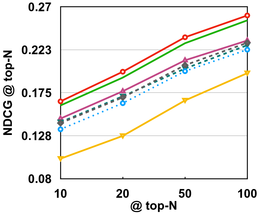
(a) NDCG@topN in Video Games

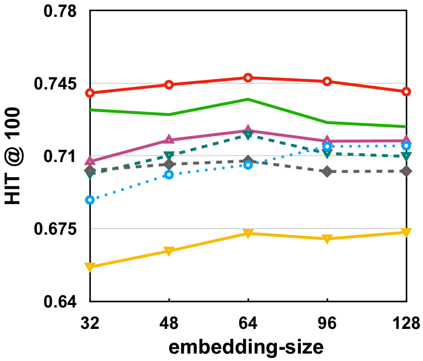
(b) HIT@100 in Yelp.

Figure 4. Performance of our models and the top-5 baselines when varying a top-N recommendation list (left) and an embedding size (right).

6.4.3. RQ2: Effect of the long-term and short-term encoding components?

Using reported results in Table 2, we first compare long-term encoding models (i.e. (a)-(d), and QUALE, AQUALE) with short-term encoding models (i.e. (e)-(h), and QUASE, AQUASE). In general, long-term encoding models work better than short-term encoding models. For instance, NAIS (i.e. best long-term encoding baseline) improves 8.5% on average on six datasets compared with Caser (i.e. best short-term encoding baseline). Similarly, our long-term encoding QUALE model works better than our short-term encoding QUASE model, enhancing 9.2% on average over six datasets. To investigate this phenomenon, we plot the density distribution of item-item similarity scores in test sets of two datasets Pet-Supplies and Yelp in Figure 5. We observe higher peaks on long-term item-item relationships in the curves, explaining why long-term encoding models work better than short-term encoding models.

Next, we compare the fused models with models that encode either long-term or short-term users preferences. Table 2 shows that models, which consider both user’s long-term and short-term preferences, work better than other models, which encode either user’s long-term or short-term interests. Both (j) and (k) baselines generally work better than (a)–(h) baselines. Specifically, our QUALSE and AQUALSE models improve 7.9%$\sim$10.0% on average over six datasets compared to the best baseline from (a)–(h). These observations show the effectiveness of modeling both user’s long-term and short-term interests. Among models, which consider both user long-term and short-term interests, SASRec performed the worst compared to baselines (i)–(k) and our QUALSE and AQUALSE. This is due to the fact that SASRec models user’s long-term and short-term interests implicitly and concurrently by using the Transformer multi-head attention mechanism. But, SLi-Rec, ALSTM+AASVD, and our proposals model the two preferences explicitly and separately, and then combine them later on, increasing flexibility. Note that, although SLi-Rec employed a time-aware attentional LSTM to better model the user’s short-term preferences, our ALSTM+AASVD implementation works slightly better than SLi-Rec due to its two distinct properties: (i) the personalized self-attention in AASVD, where each user is parameterized by her own context vector, and (ii) the personalized gating fusion.

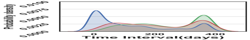
(a) Pet Supplies dataset.

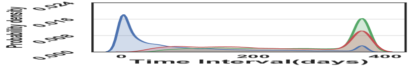
(b) Yelp dataset.

Figure 5. Density distribution of item-item similarity scores in train/vad/test sets of Pet Supplies and Yelp datasets.

6.4.4. RQ3: Is using Quaternion representation helpful?

In Table 2, we compare different model pairs: AASVD vs. QUALE, ALSTM vs. QUASE (LSTM), AGRU vs. QUASE (GRU), and ALSTM+AASVD vs. QUALSE. Two methods under the same pair have similar architecture (again, ALSTM+AASVD was implemented by us, following our QUALSE architecture to show effectiveness of Quaternion representation). But, the first method of each pair uses real-valued representations and the second method of each pair uses Quaternion representations. Table 2 shows that QUALE works better than AASVD. In six datasets, on average, QUALE improves Hit@100 by 5.60% and NDCG@100 by 7.71% compared to AASVD. Similarly, we observe the same patterns from the other three model pairs. Moreover, when comparing our long-term encoding QUALE and AQUALE models with other long-term encoding baselines (a)-(e), our models outperformed the baselines, improving HIT@100 by 5.16% and 6.55%, and enhancing NDCG@100 by 7.11% and 9.83%, respectively. Similarly, our short-term encoding QUASE and AQUASE using LSTM also work better than other short-term encoding baselines (f)-(h), improving HIT@100 by 4.75% and 8.09%, and enhancing NDCG@100 by 10.57% and 15.33%, respectively. All of these results confirm the effectiveness of modeling user’s interests by using Quaternion representations over Euclidean representations.

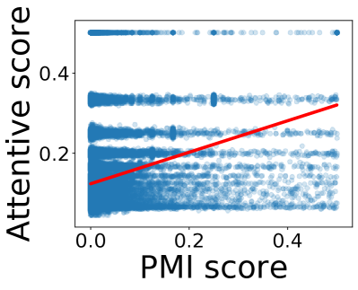
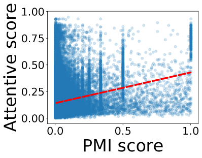
(a) QUALE vs AASVD.

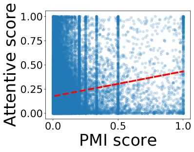
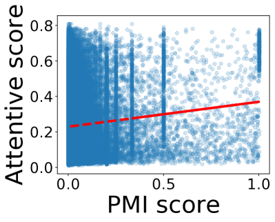
(b) QUASE vs ALSTM.

Figure 6. Comparison of attention scores between (QUALE vs AASVD) and (QUASE vs ALSTM) in the Apps for Android dataset. Pearson correlation $\rho$ between attention scores and PMI scores are: $\rho_{QUALE}=0.232>\rho_{AASVD}=0.216$, and $\rho_{QUASE}=0.148>\rho_{ALSTM}=0.1$.

Why Quaternion representations help improve the performance? Since attention mechanism is the key success in deep neural networks (Vaswani et al., 2017), we analyze how our models assign attention weights compared to their respective real-valued models. We first measure the item-item Pointwise Mutual Information (PMI) scores (i.e. $PMI(j,t)=log\frac{P(j,t)}{P(j)\times P(t)}$) using the training set. The PMI score between two items ($j,t$) gives us the co-occurrence information between item $j$ and item $t$, or how likely the target item $j$ will be preferred by the target user when the item $t$ is already in her consumed item list. We perform softmax on all item-item PMI scores. Then, we compare with the generated attention scores from our proposed models and ones from their respective real-valued baseline models. Figure 6 shows the scatter plots and Pearson correlation comparison using the Apps for Android dataset. We see that QUALE, QUASE tend to correlate more positively with the PMI scores than their respective real-valued models AASVD, ALSTM. In another word, our Quaternion-based models assign higher scores for co-occurred item pairs. We reason coming from two aspects of Quaternion representations. First, Hamilton product in Quaternion space encourages strong inter-latent interactions across Quaternion components. Second, since our proposed self-attention mechanism produces scores in Quaternion space, the output attention scores have four values w.r.t four Quaternion components. This can be thought as similar to the multi-head attention mechanism (Vaswani et al., 2017) (but not exactly same because of the weight shared in Quaternion transformation), where the proposed attention mechanism learns to attend different aspects from the four Quaternion components. All of these explain why we got better results compared to the respective real-valued models.

6.4.5. RQ4: Effect of the personalized gated fusion and the QABPR loss?

Table 2 shows that in real-valued representations, ALSTM+ASVD works better than AASVD and ALSTM in all six datasets. Similarly, in Quaternion representations, the fused QUALSE model generally works better than its two degenerated QUALE and QUASE models. In the six datasets, both QUALSE and AQUALSE perform better than their degenerated (adversarial) versions, improving 2% on average w.r.t both HIT@100 and NDCG@100. The results confirm the effectiveness of fusing long-term and short-term user preferences in both of QUALSE and AQUALSE.

We further compare our gating fusion with a weight fixing method, where we vary a contribution score $c\in[0,1]$ for the user’s short-term preference encoding part and $1-c$ for the long-term part. We see that the gating fusion improves 4.82% on average over six datasets compared to the weight fixing method, again confirming the effectiveness of our personalized gating fusion method.

Is Quaternion Adversarial training on BPR loss helpful? We compare our proposed models training with BPR loss (i.e. QUALE, QUASE (LSTM), and QUALSE models) and our proposed models training with QABPR loss (i.e. AQUALE, AQUASE (LSTM), and AQUALSE). First, we observe that AQUASE boosted QUASE performance by a large margin: improving HIT@100 by 3.2% and NDCG@100 by 4.29% on average in the six datasets. AQUALE and AQUALSE also improve QUALE and QUALSE by 1.92% and 1.91% on average of both HIT@100 and NDCG@100 over six datasets, respectively. These results show the effectiveness of the adversarial attack on Quaternion representations with our QABPR loss.

7. Conclusion

In this paper, we have shown that user’s short-term and long-term interests are complementary and both of them are indispensable. We fully utilized Quaternion space and proposed three novel Quaternion-based models: (1) a QUALE model learned the user’s long-term intents, (2) a QUASE model learned the user’s short-term interests, and (3) a QUALSE model fused QUALE and QUASE to learn both user’s long-term and short-term preferences. We also proposed a Quaternion-based Adversarial attack on Bayesian Personalized Ranking (QABPR) loss to improve the robustness of our proposals. Through extensive experiments on six real-world datasets, we showed that our QUALSE improved 6.87% at HIT@1 and 8.71% at NDCG@1, and AQUALSE improved 8.43% at HIT@1 and 10.27% at NDCG@1 on average compared with the best baseline. Our proposed models consistently achieved the best results when varying top-N (e.g., HIT@100 and NDCG@100). These results show the effectiveness of our proposed framework.

8. ACKNOWLEDGMENTS

This work was supported in part by NSF grant CNS-1755536, AWS Cloud Credits for Research, and Google Cloud.

References

- (1)
- Ebesu et al. (2018) Travis Ebesu, Bin Shen, and Yi Fang. 2018. Collaborative memory network for recommendation systems. In SIGIR. 515–524.
- Feng et al. (2015) Shanshan Feng, Xutao Li, Yifeng Zeng, Gao Cong, Yeow Meng Chee, and Quan Yuan. 2015. Personalized ranking metric embedding for next new POI recommendation. In IJCAI. 2069–2075.
- Gaudet and Maida (2018) Chase J Gaudet and Anthony S Maida. 2018. Deep quaternion networks. In IJCNN. 1–8.
- Hamilton (1844) William Rowan Hamilton. 1844. LXXVIII. On quaternions; or on a new system of imaginaries in Algebra: To the editors of the Philosophical Magazine and Journal. The London, Edinburgh, and Dublin Philosophical Magazine and Journal of Science 25, 169 (1844), 489–495.
- He et al. (2017a) Ruining He, Wang-Cheng Kang, and Julian McAuley. 2017a. Translation-based recommendation. In RecSys. 161–169.
- He and McAuley (2016) Ruining He and Julian McAuley. 2016. Ups and downs: Modeling the visual evolution of fashion trends with one-class collaborative filtering. In WWW. 507–517.
- He et al. (2018a) Xiangnan He, Zhankui He, Xiaoyu Du, and Tat-Seng Chua. 2018a. Adversarial personalized ranking for recommendation. In SIGIR. 355–364.
- He et al. (2018b) Xiangnan He, Zhankui He, Jingkuan Song, Zhenguang Liu, Yu-Gang Jiang, and Tat-Seng Chua. 2018b. NAIS: Neural attentive item similarity model for recommendation. IEEE TKDE 30, 12 (2018), 2354–2366.
- He et al. (2017b) Xiangnan He, Lizi Liao, Hanwang Zhang, Liqiang Nie, Xia Hu, and Tat-Seng Chua. 2017b. Neural collaborative filtering. In WWW. 173–182.
- He et al. (2016) Xiangnan He, Hanwang Zhang, Min-Yen Kan, and Tat-Seng Chua. 2016. Fast matrix factorization for online recommendation with implicit feedback. In SIGIR. 549–558.
- Hidasi et al. (2016) Balázs Hidasi, Alexandros Karatzoglou, Linas Baltrunas, and Domonkos Tikk. 2016. Session-based recommendations with recurrent neural networks. In ICLR.
- Hochreiter and Schmidhuber (1997) Sepp Hochreiter and Jürgen Schmidhuber. 1997. Long short-term memory. Neural computation 9, 8 (1997), 1735–1780.
- Hu et al. (2008) Yifan Hu, Yehuda Koren, and Chris Volinsky. 2008. Collaborative filtering for implicit feedback datasets. In ICDM. 263–272.
- Kabbur et al. (2013) Santosh Kabbur, Xia Ning, and George Karypis. 2013. Fism: factored item similarity models for top-n recommender systems. In KDD. 659–667.
- Kang and McAuley (2018) Wang-Cheng Kang and Julian McAuley. 2018. Self-attentive sequential recommendation. In ICDM. 197–206.
- Kingma and Ba (2015) Diederik P Kingma and Jimmy Ba. 2015. Adam: A method for stochastic optimization. In ICLR.
- Koren (2008) Yehuda Koren. 2008. Factorization meets the neighborhood: a multifaceted collaborative filtering model. In KDD. 426–434.
- Koren et al. (2009) Yehuda Koren, Robert Bell, and Chris Volinsky. 2009. Matrix factorization techniques for recommender systems. Computer 42, 8 (2009), 30–37.
- Kurakin et al. (2017) Alexey Kurakin, Ian Goodfellow, and Samy Bengio. 2017. Adversarial examples in the physical world. ICLR Workshop (2017).
- Li et al. (2017) Jing Li, Pengjie Ren, Zhumin Chen, Zhaochun Ren, Tao Lian, and Jun Ma. 2017. Neural attentive session-based recommendation. In CIKM. 1419–1428.
- Liang et al. (2018) Dawen Liang, Rahul G Krishnan, Matthew D Hoffman, and Tony Jebara. 2018. Variational autoencoders for collaborative filtering. In WWW. 689–698.
- Liu et al. (2016) Qiang Liu, Shu Wu, Diyi Wang, Zhaokang Li, and Liang Wang. 2016. Context-aware sequential recommendation. In ICDM. 1053–1058.
- Ma et al. (2019a) Chen Ma, Peng Kang, and Xue Liu. 2019a. Hierarchical gating networks for sequential recommendation. In KDD. 825–833.
- Ma et al. (2019b) Chen Ma, Peng Kang, Bin Wu, Qinglong Wang, and Xue Liu. 2019b. Gated attentive-autoencoder for content-aware recommendation. In WSDM. 519–527.
- Ma et al. (2018) Chen Ma, Yingxue Zhang, Qinglong Wang, and Xue Liu. 2018. Point-of-interest recommendation: Exploiting self-attentive autoencoders with neighbor-aware influence. In CIKM. 697–706.
- Okura et al. (2017) Shumpei Okura, Yukihiro Tagami, Shingo Ono, and Akira Tajima. 2017. Embedding-based news recommendation for millions of users. In KDD. 1933–1942.
- Parcollet et al. (2019a) Titouan Parcollet, Mohamed Morchid, and Georges Linarès. 2019a. Quaternion convolutional neural networks for heterogeneous image processing. In ICASSP. IEEE, 8514–8518.
- Parcollet et al. (2019b) Titouan Parcollet, Mirco Ravanelli, Mohamed Morchid, Georges Linarès, Chiheb Trabelsi, Renato De Mori, and Yoshua Bengio. 2019b. Quaternion recurrent neural networks. In ICLR.
- Rendle et al. (2009) Steffen Rendle, Christoph Freudenthaler, Zeno Gantner, and Lars Schmidt-Thieme. 2009. BPR: Bayesian personalized ranking from implicit feedback. In UAI. 452–461.
- Rendle et al. (2010) Steffen Rendle, Christoph Freudenthaler, and Lars Schmidt-Thieme. 2010. Factorizing personalized markov chains for next-basket recommendation. In WWW. 811–820.
- Resnick and Varian (1997) Paul Resnick and Hal R Varian. 1997. Recommender systems. Commun. ACM 40, 3 (1997), 56–58.
- Tang and Wang (2018) Jiaxi Tang and Ke Wang. 2018. Personalized top-n sequential recommendation via convolutional sequence embedding. In WSDM. 565–573.
- Tay et al. (2019) Yi Tay, Aston Zhang, Luu Anh Tuan, Jinfeng Rao, Shuai Zhang, Shuohang Wang, Jie Fu, and Siu Cheung Hui. 2019. Lightweight and efficient neural natural language processing with quaternion networks. In ACL. 1494–1503.
- Tran et al. (2018) Thanh Tran, Kyumin Lee, Yiming Liao, and Dongwon Lee. 2018. Regularizing matrix factorization with user and item embeddings for recommendation. In CIKM. 687–696.
- Tran et al. (2019a) Thanh Tran, Xinyue Liu, Kyumin Lee, and Xiangnan Kong. 2019a. Signed Distance-based Deep Memory Recommender. In WWW. 1841–1852.
- Tran et al. (2019b) Thanh Tran, Renee Sweeney, and Kyumin Lee. 2019b. Adversarial mahalanobis distance-based attentive song recommender for automatic playlist continuation. In SIGIR. 245–254.
- Vaswani et al. (2017) Ashish Vaswani, Noam Shazeer, Niki Parmar, Jakob Uszkoreit, Llion Jones, Aidan N Gomez, Łukasz Kaiser, and Illia Polosukhin. 2017. Attention is all you need. In NeurIPS. 5998–6008.
- Vinh Tran et al. (2019) Lucas Vinh Tran, Tuan-Anh Nguyen Pham, Yi Tay, Yiding Liu, Gao Cong, and Xiaoli Li. 2019. Interact and decide: Medley of sub-attention networks for effective group recommendation. In SIGIR. 255–264.
- Wang et al. (2019) Xiang Wang, Xiangnan He, Meng Wang, Fuli Feng, and Tat-Seng Chua. 2019. Neural graph collaborative filtering. In SIGIR. 165–174.
- Wu et al. (2017) Chao-Yuan Wu, Amr Ahmed, Alex Beutel, Alexander J Smola, and How Jing. 2017. Recurrent recommender networks. In WSDM. 495–503.
- Xin et al. (2019) Xin Xin, Xiangnan He, Yongfeng Zhang, Yongdong Zhang, and Joemon Jose. 2019. Relational collaborative filtering: Modeling multiple item relations for recommendation. In SIGIR. 125–134.
- Yu et al. (2019) Zeping Yu, Jianxun Lian, Ahmad Mahmoody, Gongshen Liu, and Xing Xie. 2019. Adaptive user modeling with long and short-term preferences for personalized recommendation. In IJCAI. 4213–4219.
- Zhang et al. (2016) Hanwang Zhang, Fumin Shen, Wei Liu, Xiangnan He, Huanbo Luan, and Tat-Seng Chua. 2016. Discrete collaborative filtering. In SIGIR. 325–334.
- Zhang et al. (2019) Shuai Zhang, Lina Yao, Lucas Vinh Tran, Aston Zhang, and Yi Tay. 2019. Quaternion Collaborative Filtering for Recommendation. In IJCAI. 4313–4319.
- Zhong et al. (2018) Victor Zhong, Caiming Xiong, and Richard Socher. 2018. Global-Locally Self-Attentive Encoder for Dialogue State Tracking. In ACL. 1458–1467.
- Zhou et al. (2019) Guorui Zhou, Na Mou, Ying Fan, Qi Pi, Weijie Bian, Chang Zhou, Xiaoqiang Zhu, and Kun Gai. 2019. Deep interest evolution network for click-through rate prediction. In AAAI, Vol. 33. 5941–5948.
- Zhu et al. (2018) Xuanyu Zhu, Yi Xu, Hongteng Xu, and Changjian Chen. 2018. Quaternion convolutional neural networks. In ECCV. 631–647.