Linear Gaussian Quantum State Smoothing: Understanding
the optimal unravelings for Alice to estimate Bob’s state

Abstract

Quantum state smoothing is a technique to construct an estimate of the quantum state at a particular time, conditioned on a measurement record from both before and after that time. The technique assumes that an observer, Alice, monitors part of the environment of a quantum system and that the remaining part of the environment, unobserved by Alice, is measured by a secondary observer, Bob, who may have a choice in how he monitors it. The effect of Bob’s measurement choice on the effectiveness of Alice’s smoothing has been studied in a number of recent papers. Here we expand upon the Letter which introduced linear Gaussian quantum (LGQ) state smoothing [Phys. Rev. Lett., 122, 190402 (2019)]. In the current paper we provide a more detailed derivation of the LGQ smoothing equations and address an open question about Bob’s optimal measurement strategy. Specifically, we develop a simple hypothesis that allows one to approximate the optimal measurement choice for Bob given Alice’s measurement choice. By ‘optimal choice’ we mean the choice for Bob that will maximize the purity improvement of Alice’s smoothed state compared to her filtered state (an estimated state based only on Alice’s past measurement record). The hypothesis, that Bob should choose his measurement so that he observes the back-action on the system from Alice’s measurement, seems contrary to one’s intuition about quantum state smoothing. Nevertheless we show that it works even beyond a linear Gaussian setting.

I Introduction

In parameter estimation, the task is to estimate unknown parameters, denoted by a vector ${\bf x}$, from available information such as measurement records. A powerful tool for parameter estimation is the probability density function (PDF), often called the state of the system, as it is possible to compute from this any estimate of ${\bf x}$, e.g., the mean or the mode of the PDF. This turns the problem into one of state estimation. There are numerous techniques for classical state estimation. Specifically, for continuous measurements, there are the techniques of filtering and smoothing Weinert (2001); Haykin (2001); Brown and Hwang (2012); Einicke (2012); Friedland (2012); Trees and Bell (2013) for classical states. Filtering uses any measurement information prior to the estimation time $\tau$, the ‘past’ measurement record $\overleftarrow{\color[rgb]{0,0,0}\rm O}$, to estimate the state of the system, yielding the filtered state $\wp_{\text{F}}({\bf x}):=\wp({\bf x}|\overleftarrow{\color[rgb]{0,0,0}\rm O})$. The complement to the filtered state is the retrofiltered effect $E_{\text{R}}({\bf x}):=\wp(\overrightarrow{\color[rgb]{0,0,0}\rm O}|{\bf x})$, more commonly referred to as the likelihood function Einicke (2012); Brown and Hwang (2012); Särkkä (2013) for the future measurement record $\overrightarrow{\color[rgb]{0,0,0}\rm O}$ given ${\bf x}$. The estimation technique of smoothing combines the filtered state and retrofiltered effect to obtain a smoothed state $\wp_{\text{S}}({\bf x}):=\wp({\bf x}|\overleftrightarrow{\color[rgb]{0,0,0}\rm O})\propto E_{\text{R}}({\bf x})\wp_{\text{F}}({\bf x})$, conditioned on both past and future measurement records, the ‘past-future’ measurement record $\overleftrightarrow{\color[rgb]{0,0,0}\rm O}$. While smoothing may be inapplicable for some purposes, as it requires information after the estimation time, it is a more accurate estimation technique for data post-processing than filtering as it utilises more information.

As we make the transition to quantum technologies, it becomes increasingly important to estimate the quantum state $\rho$ of a system. There are well-known techniques to estimate quantum state preparation from an ensemble of measurement results, e.g., tomography D’Ariano et al. (2003). Here, however, we are interested in techniques using a single realization of a continuous measurement record, such as quantum trajectory theory Belavkin (1987, 1992); Wiseman and Milburn (2010). This technique is analogous to the classical technique of filtering in that it only uses the past measurement record to obtain the filtered quantum state $\rho_{\text{F}}(\tau)$. As in the classical case, the complement of the filtered quantum state is the retrofiltered quantum effect $\hat{E}_{\text{R}}(\tau)$, a positive operator defined such that $\text{Tr}[\hat{E}_{\text{R}}\rho]=\wp(\overrightarrow{\color[rgb]{0,0,0}\rm O}|\rho)$.

For the quantum analog of smoothing, it is not as simple as combining the filtered state and the retrofiltered effect as it was in the classical case. If we were to combine them following the pattern of the classical case, $\varrho(\tau)\propto\rho_{\text{F}}(\tau)\hat{E}_{\text{R}}(\tau)$, the resulting operator would not be a valid quantum state. That is in general, the operator is not positive semidefinite Tsang (2009a, b); Gammelmark et al. (2013); Guevara and Wiseman (2015); Ohki (2015); Tsang (2019); Laverick et al. (2020). We do not want to give the reader the impression that this operator is useless; in fact, it has an interesting connection to weak values Aharonov et al. (1964, 1988); Tsang (2009b). Consequently, a symmetrized version of $\varrho(\tau)$ has been referred to as the smoothed weak-value (SWV) state $\varrho_{\rm SWV}$ Laverick et al. (2019, 2020).

There is, however, a quantum state smoothing formalism developed by Guevara and Wiseman Guevara and Wiseman (2015) which guarantees a valid smoothed quantum state. The formalism considers a quantum system partially observed by an observer, Alice, whose task is to estimate the true state of the systems using only her observed record. However, for Alice to obtain a valid smoothed quantum state, that is, a state conditioned on her past-future measurement record, it is necessary to introduce a secondary observer, say Bob, who gathers all information unobserved by Alice, see Fig. 1. By using both Alice’s and Bob’s measurement records to estimate the quantum state, we would obtain the true quantum state, a state containing maximal information about the quantum system. The true state is crucial to calculating the smoothed state.

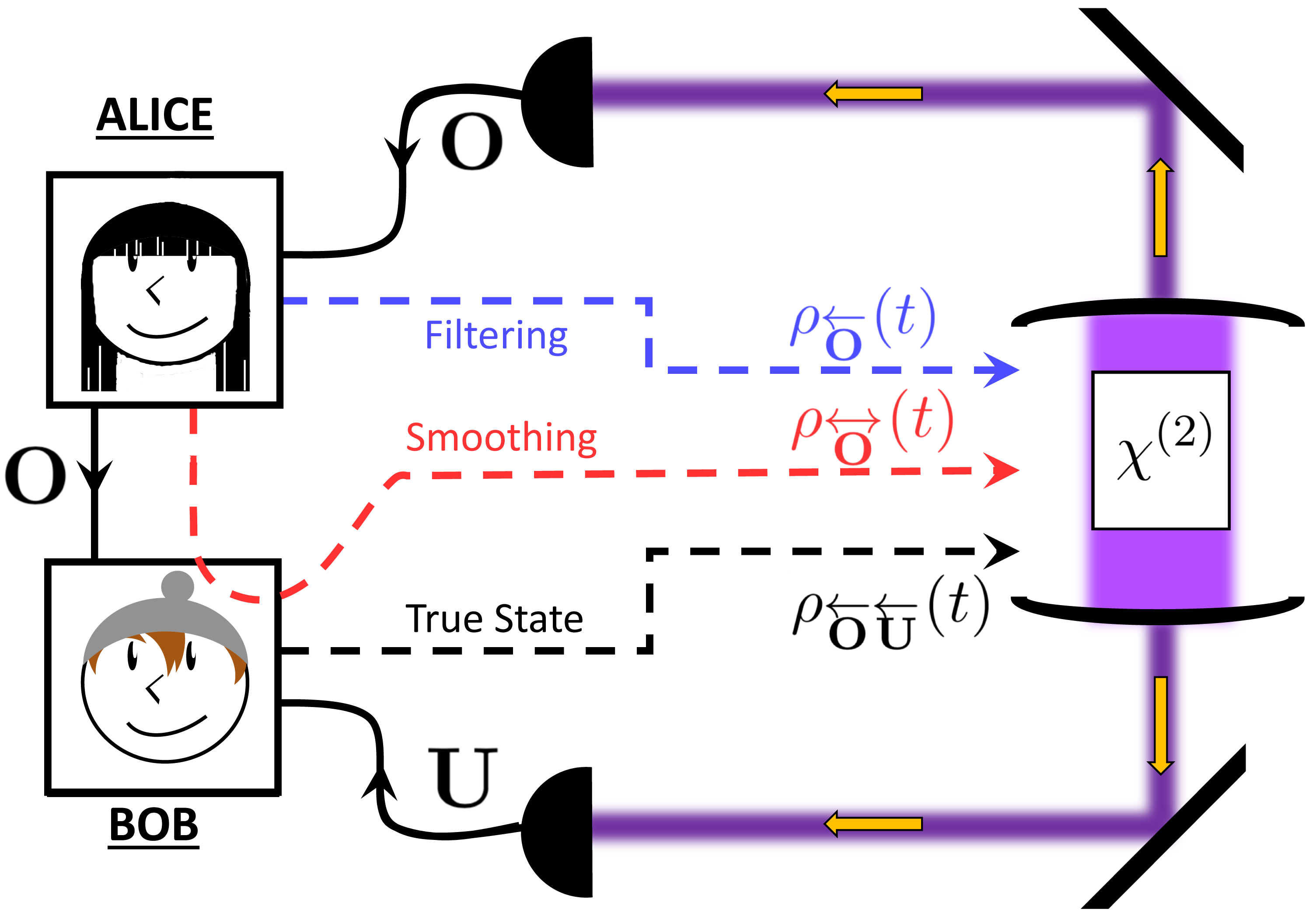
Figure 1: A diagrammatic representation of the quantum state smoothing formalism. Bob, who has access to both the observed record ${\color[rgb]{0,0,0}\rm O}$ and the unobserved record ${\color[rgb]{0,0,0}\rm U}$, is able to obtain the best estimate of the quantum state, the true state $\rho_{\text{T}}:=\rho_{\overleftarrow{\color[rgb]{0,0,0}\rm O}\overleftarrow{\color[rgb]{0,0,0}\rm U}}$ of the quantum system ${\cal Q}$. Alice, on the other hand has access to only the observed record ${\color[rgb]{0,0,0}\rm O}$. If Alice does not know of the existence of the ${\color[rgb]{0,0,0}\rm U}$, then her best estimate would be the filtered estimate $\rho_{\text{F}}:=\rho_{\overleftarrow{\color[rgb]{0,0,0}\rm O}}$. However, if Alice knows the measurement setting Bob used to obtain ${\color[rgb]{0,0,0}\rm U}$, she can utilise the full past-future observed record to obtain the smoothed state $\rho_{\text{S}}:=\rho_{\overleftrightarrow{\color[rgb]{0,0,0}\rm O}}$, which is a more accurate estimate of Bob’s true state than the filtered state.

The smoothed quantum state has been shown to offer a better estimate of the true state than the conventional filtered state, where the improvement is quantified by the state purity Guevara and Wiseman (2015); Laverick et al. (2019); Chantasri et al. (2019). Interestingly, the purity improvement of the smoothed state over the filtered state depends on both Alice’s and Bob’s choices of measurement on their parts of the system’s environment. Note, these choices do not affect the unconditioned system evolution, described by a master equation. This raises an interesting question: How should Alice observe and ‘unobserve’ (that is, Bob observe) the quantum system in order to obtain the maximum purity improvement for the smoothed quantum state? Recently Chantasri et al. (2019), the optimal measurement strategy for Alice and Bob has been investigated for a single qubit example. However, due to the vast number of unobserved measurement records that are needed in order to calculate the smoothed quantum state in such a system, the authors were only able to consider a handful of measurement scenarios.

Since the original proposal in 2015 Guevara and Wiseman (2015), the quantum state smoothing theory has been adapted by the present authors to linear Gaussian quantum (LGQ) systems Laverick et al. (2019). Thanks to the nice properties of LGQ systems, the theory of Ref. Laverick et al. (2019) provided simple closed-form solutions for the smoothed quantum state, enabling its properties to be investigated either analytically or semianalytically Laverick et al. (2019, 2020). If we restrict our analysis to LGQ systems, though we are also restricting to diffusive-type unravelings of the system, we can drastically increase the number of measurement scenarios for Alice and Bob in the search for the optimal measurement strategy. As a result, we can numerically determine the optimal diffusive measurement scenario for Alice and Bob for any type of LGQ system. But can we understand the results intuitively?

In this paper, we first review the necessary theory required for LGQ state smoothing, and provide a more detailed derivation of the theory than that presented in Ref. Laverick et al. (2019). We then present numerically simulated LGQ trajectories, showing their means and covariances, of the filtered, SWV, and smoothed quantum states. This is to observe the differences in these estimators and analyze their properties as a function of time. As expected, we observe that the smoothed quantum state estimates the true state better than the filtered state could. The SWV state, on the other hand, performs very differently.

As the main focus of this paper, we present three possible hypotheses for the optimal measurement strategy for Alice and Bob, and study how well they predict the optimal measurements found numerically for two LGQ physical systems: an on-threshold optical parametric oscillator and a stochastic linear attenuator. The most successful strategy has a surprisingly counter intuitive logic to it. Lastly, we generalize the logic behind the most successful hypotheses from the LGQ setting to the qubit setting by defining analogous quantities for a driven qubit measured using homodyne detections. Moreover, we find that the success of the counter intuitive strategy is replicated in the qubit system.

The structure of this paper is as follows. In Sec. II we will briefly review the classical linear Gaussian (LG) state estimation. Then, in Sec. III we review LGQ systems along with the LGQ state smoothing theory. Next, in Sec. IV we introduce the two physical systems that we will consider throughout the paper. We simulate the trajectories for the filtered, true, SWV, and smoothed quantum states in Sec. V. Finally, in Sec. VI we find a simple hypothesis for the best measurement strategy for Alice and Bob to maximize the purity of the smoothed state compared to the filtered state, which works for our two LGQ examples and, suitably generalized, for a very different qubit example.

II Classical LG State Estimation

For a classical dynamical system, a state of knowledge of the system is defined as the PDF $\wp({\color[rgb]{0,0,0}{\check{\bf x}}})$, where ${\color[rgb]{0,0,0}{\check{\bf x}}=(\check{x}_{1},\check{x}_{2},...,\check{x}_{D})\!^{\top}}$ is the vector of $D$ parameters required to completely describe the system, with $\top$ denoting the transpose. Note, we have used the wedge mark on ${\color[rgb]{0,0,0}{\check{\bf x}}}$ to make it clear that this is a dummy variable for the PDF and not the corresponding random variable which we denote by ${\bf x}$. We will restrict our analysis to Gaussian states, $\wp({\check{\bf x}})=g({\check{\bf x}};\langle{{\bf x}}\rangle,V)$. That is, the state is specified by its mean $\langle{{\bf x}}\rangle$ and covariance matrix $V=\langle{{\bf x}{\bf x}^{\top}}\rangle-\langle{{\bf x}}\rangle\langle{{\bf x}}\rangle\!^{\top}$. In order to guarantee that the state remains Gaussian throughout its evolution even when conditioned on continuous observation, the system must be initialized in a Gaussian state and must satisfy the following constraints Wiseman and Milburn (2010); Haykin (2001); Weinert (2001); Trees and Bell (2013); Brown and Hwang (2012); Einicke (2012); Friedland (2012). First, the system’s dynamical evolution must be described by a linear Langevin equation

$${\rm d}{\bf x}=A{\bf x}{\rm d}t+E{\rm d}{\bf v}_{\text{p}}\,.$$ (1)

Here $A$ and $E$ are constant matrices and ${\rm d}{\bf v}_{\text{p}}$ is the process noise, which is a vector of independent Wiener increments that satisfies

$$\mathbb{E}[{\rm d}{\bf v}_{\text{p}}]={\bf 0}\,,\qquad{\rm d}{\bf v}_{\text{p}}({\rm d}{\bf v}_{\text{p}})\!^{\top}\!=I{\rm d}t\,,$$ (2)

where $\mathbb{E}[...]$ denotes an ensemble average over all possible realisations of the noise. The second constraint is that any measurement record obtained must be linear in ${\bf x}$, i.e.,

$${\bf y}{\rm d}t=C{\bf x}{\rm d}t+{\rm d}{\bf v}_{\text{m}},$$ (3)

where $C$ is a constant matrix and ${\rm d}{\bf v}_{\text{m}}$ is the measurement noise, a vector of independent increments satisfying similar conditions to Eq. (2). There may exist some correlations between the measurement noise and the process noise of the system, for example, from measurement back-action, which can be described by a cross-correlation matrix $\Gamma^{\top}{\rm d}t=E{\rm d}{\bf v}_{\text{p}}({\rm d}{\bf v}_{\text{m}})\!^{\top}$ Wiseman and Milburn (2010). We will note that the majority of classical texts Weinert (2001); Haykin (2001); Brown and Hwang (2012); Einicke (2012); Friedland (2012); Trees and Bell (2013) on this topic assume that $\Gamma=0$.

The classical LG systems are defined by the above constraints. We can condition the estimate of the LG state on the past measurement record to obtain the filtered estimate $\wp_{\text{F}}({\check{\bf x}})=g({\check{\bf x}},\langle{{\bf x}}\rangle_{\text{F}},V_{\text{F}})$, whose mean and covariance are given by the Kalman-Bucy filtering equations Wiseman and Milburn (2010); Kailath and Frost (1968); Kailath (1970, 1973); Badawi et al. (1979)

$${\rm d}\langle{{\bf x}}\rangle_{\text{F}}=\,A\langle{{\bf x}}\rangle_{\text{F}}{\rm d}t+{\cal K}^{+}[V_{\text{F}}]{\rm d}{\bf w}_{\text{F}}\,,$$ (4)

$$\frac{{\rm d}V_{\text{F}}}{{\rm d}t}=\,AV_{\text{F}}+V_{\text{F}}A^{\top}\!+D-{\cal K}^{+}[V_{\text{F}}]{\cal K}^{+}[V_{\text{F}}]^{\top}\,,$$ (5)

with initial conditions $\langle{{\bf x}}\rangle_{\text{F}}(t_{0})=\langle{{\bf x}}\rangle_{0}$ and $V_{\text{F}}(t_{0})=V_{0}$. Here, ${\rm d}{\bf w}_{\text{F}}:={\bf y}{\rm d}t-C\langle{{\bf x}}\rangle_{\text{F}}{\rm d}t$ is a vector of innovations, $D=EE^{\top}$ is the diffusion matrix, and

$${\cal K}^{\pm}[V]:=VC^{\top}\!\pm\Gamma^{\top}$$ (6)

is the optimal Kalman gain matrix, as a function of the covariance.

As mentioned earlier, if we want to obtain a more accurate estimate of the state, we can utilise the past-future measurement record $\overleftrightarrow{\color[rgb]{0,0,0}\rm O}$ as opposed to the past record $\overleftarrow{\color[rgb]{0,0,0}\rm O}$ the filtered state uses. The smoothed state obtained by using $\overleftrightarrow{\color[rgb]{0,0,0}\rm O}$ can be calculated using the filtered state according to

$$\wp_{\text{S}}({\color[rgb]{0,0,0}{\check{\bf x}}}):=\wp({\color[rgb]{0,0,0}{\check{\bf x}}}|\overleftrightarrow{\color[rgb]{0,0,0}\rm O})\propto E_{\text{R}}({\color[rgb]{0,0,0}{\check{\bf x}}})\wp_{\text{F}}({\color[rgb]{0,0,0}{\check{\bf x}}})\,,$$ (7)

where we have assumed that the system is Markovian. To explicitly see the dependence on the measurement records, we remind the reader that the filtered state is a function of the past measurement record, $\wp_{\text{F}}({\check{\bf x}}):=\wp({\check{\bf x}}|\overleftarrow{\color[rgb]{0,0,0}\rm O})$. The retrofiltered effect is the likelihood of a particular realization of a future measurement record occurring from a configuration ${\color[rgb]{0,0,0}{\check{\bf x}}}$, i.e., $E_{\text{R}}({\color[rgb]{0,0,0}{\check{\bf x}}}):=\wp(\overrightarrow{\color[rgb]{0,0,0}\rm O}|{\color[rgb]{0,0,0}{\check{\bf x}}})$. Using Bayes’ theorem Jazwinski (2007) results in Eq. (7). As we already have calculated the filtered state, all we need to calculate to obtain the smoothed state is the retrofiltered effect.

If we apply Bayes’ theorem to the retrofiltered effect, we obtain $E_{\text{R}}({\color[rgb]{0,0,0}{\check{\bf x}}})\propto\wp({\color[rgb]{0,0,0}{\check{\bf x}}}|\overrightarrow{\color[rgb]{0,0,0}\rm O})\wp(\overrightarrow{\color[rgb]{0,0,0}\rm O})$. As we are using the retrofiltered effect to calculate the smoothed state, the future measurement record will be fixed and the probability $\wp(\overrightarrow{\color[rgb]{0,0,0}\rm O})$ for that fixed record will be a constant. As a result, the retrofiltered effect is $E_{\text{R}}({\color[rgb]{0,0,0}{\check{\bf x}}})\propto\wp({\color[rgb]{0,0,0}{\check{\bf x}}}|\overrightarrow{\color[rgb]{0,0,0}\rm O})$, from which we can define a normalised retrofiltered effect $E_{\text{R}}^{\prime}({\color[rgb]{0,0,0}{\check{\bf x}}})=\wp({\color[rgb]{0,0,0}{\check{\bf x}}}|\overrightarrow{\color[rgb]{0,0,0}\rm O})$. As we are limiting our discussion to Gaussian systems, the normalized retrofiltered effect will be a Gaussian, $E^{\prime}_{\text{R}}({\color[rgb]{0,0,0}{\check{\bf x}}})=g({\color[rgb]{0,0,0}{\check{\bf x}}};\langle{{\bf x}}\rangle_{\text{R}},V_{\text{R}})$, where the retrofiltered mean $\langle{{\bf x}}\rangle_{\text{R}}$ and corresponding covariance matrix $V_{\text{R}}$ are given by

$$-{\rm d}\langle{{\bf x}}\rangle_{\text{R}}=-A\langle{{\bf x}}\rangle_{\text{R}}{\rm d}t+{\cal K}^{-}[V_{\text{R}}]{\rm d}{\bf w}_{\text{R}},$$ (8)

$$-\frac{{\rm d}V_{\text{R}}}{{\rm d}t}=-AV_{\text{R}}-V_{\text{R}}A^{\top}\!+D-{\cal K}^{-}[V_{\text{R}}]{\cal K}^{-}[V_{\text{R}}]^{\top}.$$ (9)

Here ${\rm d}{\bf w}_{\text{R}}={\bf y}{\rm d}t-C\langle{{\bf x}}\rangle_{\text{R}}{\rm d}t$ and ${\cal K}^{-}[V_{\text{R}}]$ is defined in Eq. (6). These retrofiltering equations evolve backwards in time, as evident from the negative sign on the left-hand side of both equations, from a final uninformative state with $V_{\text{R}}(T)=\infty$. However, due to the infinite final retrofiltered covariance, there is no sensible final condition for the retrofiltered mean.

One can obtain more practical equations Fraser (1967), which can be used in numerical computations and the upcoming SWV state, by instead solving for the inverse retrofiltered covariance $\Lambda_{\text{R}}=V_{\text{R}}^{-1}$, referred to as an information matrix, and defining a new ‘informative’ mean ${\bf z}_{\text{R}}=\Lambda_{\text{R}}\langle{{\bf x}}\rangle_{\text{R}}$. Using the identity

$$\frac{{\rm d}}{{\rm d}t}V^{-1}=-V^{-1}\frac{{\rm d}V}{{\rm d}t}V^{-1}\,,$$ (10)

we obtain the equations for the retrofiltered informative mean and the information matrix

$$-{\rm d}{\bf z}_{\text{R}}=(\tilde{A}-\tilde{D}\Lambda_{\text{R}})\!^{\top}{\bf z}_{\text{R}}{\rm d}t+(C^{\top}\!-\Lambda_{\text{R}}\Gamma^{\top}){\bf y}{\rm d}t\,,$$ (11)

$$-\frac{{\rm d}\Lambda_{\text{R}}}{{\rm d}t}=\Lambda_{\text{R}}\tilde{A}+\tilde{A}^{\top}\!\Lambda_{\text{R}}-\Lambda_{\text{R}}\tilde{D}\Lambda_{\text{R}}+C^{\top}\!C\,,$$ (12)

with $\tilde{A}=A-\Gamma^{\top}\!C$ and $\tilde{D}=D-\Gamma^{\top}\Gamma$. We can now simply set the final conditions to be ${\bf z}_{\text{R}}(T)=0$ and $\Lambda_{\text{R}}(T)=0$.

Finally, now that we have equations for both the filtered state and the retrofiltered effect, we can compute the smoothed state using Eq. (7). Due to the proportionalilty in Eq. (7), we can replace the retrofiltered effect $E_{\text{R}}({\color[rgb]{0,0,0}{\check{\bf x}}})$ with its normalized counterpart $E_{\text{R}}^{\prime}({\color[rgb]{0,0,0}{\check{\bf x}}})$, as any proportionality constants will be accounted for during the normalization process. Since both the filtered state and retrofiltered effect are Gaussians, then by the multiplicative property of Gaussians, the smoothed state will also be Gaussian. That is, $\wp_{\text{S}}({\color[rgb]{0,0,0}{\check{\bf x}}})=g({\color[rgb]{0,0,0}{\check{\bf x}}};\langle{{\bf x}_{\text{S}}}\rangle,V_{\text{S}})$, with smoothed mean and covariance Weinert (2001); Einicke (2012); Särkkä (2013); Mayne (1966); Fraser (1967); Fraser and Potter (1969)

$$\langle{{\bf x}}\rangle_{\text{S}}=V_{\text{S}}\left[V_{\text{F}}^{-1}\langle{{\bf x}}\rangle_{\text{F}}+V_{\text{R}}^{-1}\langle{{\bf x}}\rangle_{\text{R}}\right]\,,$$ (13)

$$V_{\text{S}}=\left[V_{\text{F}}^{-1}+V_{\text{R}}^{-1}\right]^{-1}.$$ (14)

Using the definition of the retrofiltered informative mean and information matrix in Eqs. (11)–(12), the equations can be simplified to

$$\langle{{\bf x}}\rangle_{\text{S}} =V_{\text{S}}\left[V_{\text{F}}^{-1}\langle{{\bf x}}\rangle_{\text{F}}+{\bf z}_{\text{R}}\right]\,,$$ (15)

$$V_{\text{S}} =\left[V_{\text{F}}^{-1}+\Lambda_{\text{R}}\right]^{-1}.$$ (16)

We can see that the smoothed state is more accurate than the filtered state through the covariances, where it is simple to see that $V_{\text{F}}\geq V_{\text{S}}$ in the $N=1$ case.

III LGQ State Estimation

III.1 Unconditioned Quantum State

In the quantum state estimation, we are concerned with estimating a density operator $\rho$ of a quantum system as opposed to a PDF $\wp({\color[rgb]{0,0,0}{\check{\bf x}}})$. For an open quantum system, the evolution of the state $\rho$, without observation, is governed by the Lindblad master equation $\hbar\dot{\rho}={\cal L}\rho$, with the initial condition $\rho(t_{0})=\rho_{0}$, where the Lindbladian superoperator ${\cal L}$ is

$$\quad{\cal L}\bullet=-i[\hat{H},\bullet]+{\cal D}[\hat{\bf c}]\bullet\,.$$ (17)

Here the Hamiltonian $\hat{H}$ describes the unitary dynamics of the system and $\hat{\bf c}\equiv(\hat{c}_{1},\hat{c}_{2},...,\hat{c}_{M})\!^{\top}$ is the vector of Lindblad operators describing the interacting channels between the system and the environment. It will also be useful to define the row vector form of $\hat{\bf c}$, which we denote by $\hat{\bf c}^{\top}\!=(\hat{c}_{1},\hat{c}_{2},...,\hat{c}_{M})$, where the reader should notice that the transpose does not act on the operators within the vector. Furthermore, the conjugate transpose is defined as the row vector $\hat{\bf c}^{\dagger}=(\hat{c}_{1}^{\dagger},\hat{c}_{2}^{\dagger},...,\hat{c}_{M}^{\dagger})$. Thus to obtain a column vector form for $\hat{\bf c}^{\dagger}$, we need to take the transpose. To denote this we will adopt the double dagger notation of Ref. Chia and Wiseman (2011), i.e., $\hat{\bf c}^{\ddagger}=(\hat{c}_{1}^{\dagger},\hat{c}_{2}^{\dagger},...,\hat{c}_{M}^{\dagger})\!^{\top}$. We can now express the nonunitary part of Eq. (17) as

$${\cal D}[\hat{\bf c}]\bullet=\hat{\bf c}^{\top}\!\!\bullet\hat{\bf c}^{\ddagger}-\{\hat{\bf c}^{\dagger}\hat{\bf c}/2,\bullet\}\,,$$ (18)

where $\{A,B\}=AB+BA$ is the anticommutator. Without monitoring the environment to gain information about the quantum system, a solution to Eq. (17) is the most accurate estimate of the system’s quantum state.

We now assume that we can describe the quantum system by $N$ bosonic modes. From this we define a vector of $2N$ operators $\hat{\bf x}=(\hat{q}_{1},\hat{p}_{1},...,\hat{q}_{N},\hat{p}_{N})\!^{\top}$, where $\hat{q}_{k}$ and $\hat{p}_{k}$ are the canonical position and conjugate momentum operators, respectively, describing the $k$th bosonic mode and satisfying the commutation relation $[\hat{q}_{k},\hat{p}_{l}]=i\hbar\delta_{kl}$. Furthermore, we assume that the system’s Hamiltonian is quadratic and the vector of Lindblad operators is linear in $\hat{\bf x}$, i.e., $\hat{H}=\hat{\bf x}^{\top}G\hat{\bf x}/2$ and $\hat{\bf c}=(I_{N},iI_{N})\bar{C}\hat{\bf x}$, where $G$ and $\bar{C}$ are constant real matrices and $I_{n}$ denotes an $n\times n$ identity matrix. These assumptions ensure that a state initially prepared in a Gaussian state will remain Gaussian throughout the evolution. By a Gaussian state we mean one whose Wigner function is Gaussian, $W({\check{\bf x}})=g({\check{\bf x}};\langle{\hat{\bf x}}\rangle,V)$, with mean $\langle{\hat{\bf x}}\rangle$ and covariance $V$. The mean and covariance are defined as $\langle{\hat{x}_{k}}\rangle=\text{Tr}[\hat{x}_{k}\rho]$ and $V_{k,l}=\text{Tr}[\{\hat{x}_{k}\hat{x}_{l}+\hat{x}_{l}\hat{x}_{k}\}\rho/2]-\langle{\hat{x}_{k}}\rangle\langle{\hat{x}_{l}}\rangle$, respectively, where $\hat{x}_{k}$ is an element of $\hat{\bf x}$. For any state $\rho$ the covariance matrix will satisfy the Schrödinger-Heisenberg uncertainty relation Wiseman and Milburn (2010),

$$V+i\hbar\Sigma/2\geq 0\,,$$ (19)

where $\Sigma_{kl}=-i[\hat{x}_{k},\hat{x}_{l}]/\hbar$ is a real symplectic matrix.

With these assumptions we can calculate the evolution of the unconditioned LGQ state via its mean and covariance,

$${\rm d}{\langle{\hat{\bf x}}\rangle}=A{\langle{\hat{\bf x}}\rangle}{\rm d}t,$$ (20)

$$\frac{{\rm d}V}{{\rm d}t}=AV+VA^{\top}\!+D\,,$$ (21)

with the initial conditions for the mean and covariance $\langle{\hat{\bf x}}\rangle(t_{0})=\langle{\hat{\bf x}}\rangle_{0}$ and $V(t_{0})=V_{0}$, respectively. Here the drift and diffusion matrices are Wiseman and Milburn (2010)

$$A=\Sigma(G+\bar{C}^{\top}\!S\bar{C})\,,\qquad D=\hbar\Sigma\bar{C}^{\top}\bar{C}\Sigma^{\top}\,,$$ (22)

respectively, with $S=\left[\begin{smallmatrix}0&I_{N}\\ -I_{N}&0\end{smallmatrix}\right]$ being another symplectic matrix.

III.2 Filtered Quantum State

In order to obtain a better estimate of the system’s state than the unconditioned state, we need to gain more information about the system by measuring the environment. In this work we focus on diffusive-type unravelings of the master equation as opposed to a jump unraveling, as the former preserves Gaussian states. The corresponding stochastic master equation, sometimes referred to as a quantum filtering equation Belavkin (1987, 1992) for reasons that will become apparent, in the $M$ representation Chia and Wiseman (2011) is

$$\hbar{\rm d}\rho_{\text{F}}={\cal L}\rho_{\text{F}}{\rm d}t+\sqrt{\hbar}{\rm d}{\bf w}_{\text{F}}^{\top}{\cal H}[M^{\dagger}\hat{\bf c}]\rho_{\text{F}}\,.$$ (23)

Here, ${\cal H}[\hat{\bf a}]\bullet=\hat{\bf a}\bullet+\bullet\hat{\bf a}^{\ddagger}-\text{Tr}[\bullet(\hat{\bf a}+\hat{\bf a}^{\ddagger})]\bullet$, and the initial condition is $\rho_{\text{F}}(t_{0})=\rho_{0}$. We have also implicitly introduced a vector of measurement currents ${\bf y}{\rm d}t=\langle M^{\dagger}\hat{\bf c}+M^{\top}\hat{\bf c}^{\ddagger}\rangle_{\text{F}}{\rm d}t+{\rm d}{\bf w}_{\text{F}}$ where $\langle{\bullet}\rangle_{\text{F}}:=\text{Tr}[\bullet\rho_{\text{F}}]$ through the vector of innovations ${\rm d}{\bf w}_{\text{F}}$, which satisfies similar conditions to Eq. (2).

To ensure that evolution under Eq. (23) does not result in an invalid quantum state, it is necessary and sufficient Chia and Wiseman (2011) for $M$ to satisfy $MM^{\dagger}={\rm diag}(\eta_{1},\eta_{2},...,\eta_{M})$, where $\eta_{k}$ can be interpreted as the monitoring efficiency of the channel $\hat{c}_{k}$. Note, we can also define an un-normalized filtered state $\tilde{\rho}_{\text{F}}$, which explicitly depends on the measurement results ${\bf y}{\rm d}t$ (instead of the innovation ${\rm d}{\bf w}_{\text{F}}$), reflecting the observer’s knowledge of the system. This un-normalized filtered state satisfies the stochastic master equation

$$\hbar{\rm d}\tilde{\rho}_{\text{F}}={\cal L}\tilde{\rho}_{\text{F}}{\rm d}t+\sqrt{\hbar}{\bf y}^{\top}\widetilde{\cal H}[M^{\dagger}\hat{\bf c}]\tilde{\rho}_{\text{F}}{\rm d}t\,,$$ (24)

where $\widetilde{\cal H}[\hat{\bf a}]\bullet=\hat{\bf a}\bullet+\bullet\hat{\bf a}^{\ddagger}$.

Restricting the discussion to LGQ systems, we can express the vector of measurement current as

$${\bf y}{\rm d}t=C\langle{\hat{\bf x}}\rangle_{\text{F}}{\rm d}t+{\rm d}{\bf w}_{\text{F}}\,,$$ (25)

where $C=2\sqrt{\hbar^{-1}}T^{\top}\bar{C}$, $T^{\top}\!=({\rm Re}[M^{\top}],{\rm Im}[M^{\top}])$, and ${\rm d}{\bf w}_{\text{F}}\equiv{\bf y}{\rm d}t-C\langle{\hat{\bf x}}\rangle_{\text{F}}{\rm d}t$. From the stochastic master equation in Eq. (23), we can derive the equations for the mean and covariance of the filtered state, giving

$${\rm d}\langle{\hat{\bf x}}\rangle_{\text{F}}=\,A\langle{\hat{\bf x}}\rangle_{\text{F}}{\rm d}t+{\cal K}^{+}[V_{\text{F}}]{\rm d}{\bf w}_{\text{F}}\,,$$ (26)

$$\frac{{\rm d}V_{\text{F}}}{{\rm d}t}=\,AV_{\text{F}}+V_{\text{F}}A^{\top}\!+D-{\cal K}^{+}[V_{\text{F}}]{\cal K}^{+}[V_{\text{F}}]^{\top}\,,$$ (27)

with initial conditions $\langle{{\bf x}}\rangle_{\text{F}}(t_{0})=\langle{\hat{\bf x}}\rangle_{0}$ and $V_{\text{F}}(t_{0})=V_{0}$. The optimal Kalman gain matrix, ${\cal K}^{+}[V_{\text{F}}]$, which we will later refer to as a kick matrix, is defined in Eq. (6), with the measurement back-action $\Gamma=-\sqrt{\hbar}T^{\top}\!S\bar{C}\Sigma^{\top}$. Note that these equations for the filtered quantum state have exactly the same form as the classical Kalman-Bucy filtering equations.

III.3 Retrofiltered Effect and Smoothed Weak-value State

The retrofiltered effect gives the probability density of a measurement result occurring at a later time given a particular quantum state at the current time:

$$\wp(\overrightarrow{\color[rgb]{0,0,0}\rm O}|\rho)=\text{Tr}[\rho\hat{E}_{\text{R}}]\,,$$ (28)

where $\hat{E}_{\text{R}}$ is a function of the future record $\overrightarrow{\color[rgb]{0,0,0}\rm O}$. The effect $\hat{E}_{\text{R}}$ can be computed backward in time from a final uninformative effect $\hat{E}_{\text{R}}(T)\propto\hat{I}$. The stochastic equation for the (unnormalized) retrofiltered effect $\hat{E}_{\text{R}}$ is obtained by taking the adjoint of Eq. (24), giving

$$-\hbar{\rm d}\hat{E}_{\text{R}}={\cal L}^{\dagger}\hat{E}_{\text{R}}{\rm d}t+\sqrt{\hbar}{\bf y}\widetilde{{\cal H}}[M^{\top}\hat{\bf c}^{\ddagger}]\hat{E}_{\text{R}}{\rm d}t\,,$$ (29)

where ${\cal L}^{\dagger}$ is the adjoint of the Lindbladian superoperator. Note that Eq. (29) is not trace-preserving and evolves backward in time. Following a similar logic to that presented in the classical case, we will normalize the retrofiltered effect, as ultimately we are interested in a smoothed state which will require normalization regardless. In doing so, we obtain a normalized retrofiltered effect $\hat{E}_{\text{R}}^{\prime}$ Zhang and Mølmer (2017),

$$\begin{split}-\hbar{\rm d}\hat{E}^{\prime}_{\text{R}}={\cal L}^{\dagger}\hat{E}^{\prime}_{\text{R}}{\rm d}t-\langle{\hat{\kappa}}\rangle&{}_{\text{R}}\hat{E}^{\prime}_{\text{R}}{\rm d}t\\ +&\sqrt{\hbar}{\rm d}{\bf w}_{\text{R}}{\cal H}[M^{\top}\hat{\bf c}^{\ddagger}]\hat{E}_{\text{R}}^{\prime}\,,\end{split}$$ (30)

where ${\rm d}{\bf w}_{\text{R}}={\bf y}{\rm d}t-\langle{M^{\dagger}\hat{\bf c}+M^{\top}\hat{\bf c}^{\ddagger}}\rangle_{\text{R}}{\rm d}t$ with $\langle{\bullet}\rangle_{\text{R}}:=\text{Tr}[\bullet\hat{E}^{\prime}_{\text{R}}]$ and $\hat{\kappa}=\hat{\bf c}^{\top}\hat{\bf c}^{\ddagger}-\hat{\bf c}^{\dagger}\hat{\bf c}$.

Considering an LGQ system, the Wigner function for the normalized retrofiltered effect is a normalized Gaussian, i.e., $W_{\text{R}}({\check{\bf x}})=g({\check{\bf x}};\langle{\hat{\bf x}}\rangle_{\text{R}},V_{\text{R}})$. Consequently, we can obtain, in a similar way to the filtered case in Eqs. (26)–(27), the equations for the retrofiltered mean and covariance,

$$-{\rm d}\langle{\hat{\bf x}}\rangle_{\text{R}}=-A\langle{\hat{\bf x}}\rangle_{\text{R}}{\rm d}t+{\cal K}^{-}[V_{\text{R}}]{\rm d}{\bf w}_{\text{R}},$$ (31)

$$- \frac{{\rm d}V_{\text{R}}}{{\rm d}t}=-AV_{\text{R}}-V_{\text{R}}A^{\top}\!+D-{\cal K}^{-}[V_{\text{R}}]{\cal K}^{-}[V_{\text{R}}]^{\top}.$$ (32)

These equations completely describe the effect, with the final condition $V_{\text{R}}(T)=\infty$. Once again, there is no sensible final condition for the retrofiltered mean due to the infinite covariance. Following the same procedure presented in the classical case, we obtain Eqs. (11)–(12), where in the quantum case ${\bf z}_{\text{R}}:=\Lambda_{\text{R}}\langle{\hat{\bf x}}\rangle_{\text{R}}$.

Following the classical equations, one might think that we could obtain a Gaussian smoothed quantum state $W_{\rm SWV}({\check{\bf x}})=g({\check{\bf x}};\langle{\hat{\bf x}}\rangle_{\rm SWV},V_{\rm SWV})$, with mean $\langle{\hat{\bf x}}\rangle_{\rm SWV}$ and covariance $V_{\rm SWV}$ given by

$$\langle{\hat{\bf x}}\rangle_{\rm SWV} =V_{\rm SWV}\left[V_{\text{F}}^{-1}\langle{\hat{\bf x}}\rangle_{\text{F}}+V_{\text{R}}^{-1}\langle{\hat{\bf x}}\rangle_{\text{R}}\right]\,,$$ (33)

$$V_{\rm SWV} =\left[V_{\text{F}}^{-1}+V_{\text{R}}^{-1}\right]^{-1}.$$ (34)

While this construction might seem valid, we will show using an example in Sec. V that the SWV covariance does not always satisfy the Schrödinger-Heisenberg uncertainty relation Eq. (19), as it would if it were a valid quantum state.

The problem lies with how the classical smoothed state converts to the quantum analogue. The above procedure for Gaussian states is equivalent to taking the symmetrized product of the filtered state and the retrofiltered effect Laverick et al. (2019, 2020),

$$\varrho_{\rm SWV}=\frac{\rho_{\text{F}}\circ\hat{E}_{\text{R}}}{\text{Tr}[\rho_{\text{F}}\circ\hat{E}_{\text{R}}]}\,.$$ (35)

Here $A\circ B=(AB+BA)/2$ denotes the Jordan product Jordan (1933); Jordan et al. (1934), and the denominator $\text{Tr}[\rho_{\text{F}}\circ\hat{E}_{\text{R}}]$ ensures that the state is normalized. We are using $\varrho$ to denote the SWV state to stress that this is not a valid quantum state which is represented by a density matrix $\rho$. The reason $\varrho_{\rm SWV}$ is not a valid quantum state is because, in general, the retrofiltered effect does not commute with the filtered quantum state. As a result, the SWV state is not guaranteed to be positive semidefinite Tsang (2009b); Laverick et al. (2020). Thus we turn to quantum state smoothing theory instead.

III.4 LGQ State Smoothing

For the quantum state smoothing theory Guevara and Wiseman (2015), we consider an open quantum system coupled to two baths. In principle, each of these baths can comprise any number of physically distinct baths, but for simplicity we will consider them collectively. An observer, Alice, monitors one of the baths and is able to construct a measurement record $\color[rgb]{0,0,0}\rm O$, which we will refer to as the ‘observed’ record. A (perhaps hypothetical) secondary observer, Bob, monitors the remaining bath and constructs his own measurement record $\color[rgb]{0,0,0}\rm U$ that is unobserved by Alice, which we will call the ‘unobserved’ record. See Fig. 1. Now Bob, assumed to have access to both the observed and the unobserved record, can estimate the quantum state conditioned on both $\overleftarrow{\color[rgb]{0,0,0}\rm O}$ and $\overleftarrow{\color[rgb]{0,0,0}\rm U}$. That is, he obtains a state with maximal information about the quantum system, which can be regarded as the true state $\rho_{\text{T}}:=\rho_{\overleftarrow{\color[rgb]{0,0,0}\rm O}\overleftarrow{\color[rgb]{0,0,0}\rm U}}$. However, since Alice does not have access to $\overleftarrow{\color[rgb]{0,0,0}\rm U}$, she can only obtain an estimate of the true state based on her observed measurement record. In this case she can construct a conditioned state with the form

$$\rho_{\text{C}}=\sum_{\overleftarrow{\color[rgb]{0,0,0}\rm U}}\wp_{\text{C}}(\overleftarrow{\color[rgb]{0,0,0}\rm U})\rho_{\text{T}}\,,$$ (36)

where the conditioning ‘${\rm C}$’ depends on the amount of the observed measurement record used in the estimation. If Alice wishes to obtain a filtered state, i.e., ${\rm C}\equiv\rm{F}$, the conditioned probability distribution for the unobserved record becomes $\wp_{\text{F}}(\overleftarrow{\color[rgb]{0,0,0}\rm U})=\wp(\overleftarrow{\color[rgb]{0,0,0}\rm U}|\overleftarrow{\color[rgb]{0,0,0}\rm O})$. To obtain a smoothed state, i.e., ${\rm C}\equiv\rm{S}$, the conditional probability becomes $\wp_{\text{S}}(\overleftarrow{\color[rgb]{0,0,0}\rm U})=\wp(\overleftarrow{\color[rgb]{0,0,0}\rm U}|\overleftrightarrow{\color[rgb]{0,0,0}\rm O})$.

For LGQ state smoothing Laverick et al. (2019), the true state of the system is represented by a Gaussian Wigner function $W_{\text{T}}({\check{\bf x}})=g({\check{\bf x}};\langle{\hat{\bf x}}\rangle_{\text{T}},V_{\text{T}})$. We introduce an unobserved measurement current ${\bf y}_{\text{u}}{\rm d}t=C_{\text{u}}\langle{\hat{\bf x}}\rangle_{\text{T}}{\rm d}t+{\rm d}{\bf w}_{\text{u}}$ to account for Bob’s monitoring of the environment, in addition to Alice’s observed measurement current ${\bf y}_{\text{o}}{\rm d}t=C_{\text{o}}\langle{\hat{\bf x}}\rangle_{\text{T}}{\rm d}t+{\rm d}{\bf w}_{\text{o}}$, where ${\rm d}{\bf w}_{\text{u}}$ and ${\rm d}{\bf w}_{\text{o}}$ are the unobserved and observed innovations, respectively. The true state of the system can be obtained by conditioning the estimate on both Alice’s and Bob’s past measurement records, giving

$${\rm d}\langle{\hat{\bf x}}\rangle_{\text{T}}=A\langle{\hat{\bf x}}\rangle_{\text{T}}{\rm d}t+{\cal K}^{+}_{\text{o}}[V_{\text{T}}]{\rm d}{\bf w}_{\text{o}}+{\cal K}^{+}_{\text{u}}[V_{\text{T}}]{\rm d}{\bf w}_{\text{u}}\,,$$ (37)

$$\frac{{\rm d}V_{\text{T}}}{{\rm d}t}=AV_{\text{T}}+V_{\text{T}}A^{\top}\!+D$$

$$\qquad\qquad-{\cal K}^{+}_{\text{o}}[V_{\text{T}}]{\cal K}^{+}_{\text{o}}[V_{\text{T}}]^{\top}-{\cal K}^{+}_{\text{u}}[V_{\text{T}}]{\cal K}^{+}_{\text{u}}[V_{\text{T}}]^{\top}\,,$$ (38)

where ${\cal K}^{\pm}_{\rm r}[V]=VC^{\top}_{\rm r}\!+\Gamma^{\top}_{\rm r}$ for r $\in\{$o,u$\}$ and the initial conditions are $\langle{\hat{\bf x}}\rangle_{\text{T}}(t_{0})=\langle{\hat{\bf x}}\rangle_{0}$ and $V_{\text{T}}(t_{0})=V_{0}$. This follows trivially by extending Eqs. (26)–(27) to two measurement records.

Since we are restricting to Gaussian states, the true state depends on $\overleftarrow{\color[rgb]{0,0,0}\rm U}$ only via the mean in Eq. (37). This means that we can replace the (symbolic) summation in Eq. (36) by an integral over the true mean, so that the smoothed state (${\rm C=S}$) is given by

$$\rho_{\text{S}}=\int\wp_{\text{S}}(\langle{\hat{\bf x}}\rangle_{\text{T}})\rho_{\text{T}}(\langle{\hat{\bf x}}\rangle_{\text{T}}){\rm d}\langle{\hat{\bf x}}\rangle_{\text{T}}\,,$$ (39)

where the PDF $\wp_{\text{S}}(\langle{\hat{\bf x}}\rangle_{\text{T}})$ is for the true mean conditioned on the past-future observed record.

We can replace the smoothed state and the true state by their Wigner functions, the latter of which is replaced by a Gaussian $g({\check{\bf x}};\accentset{\raisebox{-1.0pt}{\scalebox{1.3}[0.4]{$\circ$}}}{{\bf x}},V_{\text{T}})$. Here we have defined a haloed variable $\accentset{\raisebox{-1.0pt}{\scalebox{1.3}[0.4]{$\circ$}}}{{\bf x}}=\langle{\hat{\bf x}}\rangle_{\text{T}}$ for notational simplicity. To obtain the smoothed state in Eq. (39), we convolve the true state with the conditional PDF (which is a classically smoothed LG distribution) $\wp_{\text{S}}(\accentset{\raisebox{-1.0pt}{\scalebox{1.3}[0.4]{$\circ$}}}{{\bf x}})=g(\accentset{\raisebox{-1.0pt}{\scalebox{1.3}[0.4]{$\circ$}}}{{\bf x}};\langle{\accentset{\raisebox{-1.0pt}{\scalebox{1.3}[0.4]{$\circ$}}}{{\bf x}}}\rangle_{\text{S}},\accentset{\raisebox{-1.0pt}{\scalebox{1.3}[0.4]{$\circ$}}}{V}_{\text{S}})$, where $\langle{\accentset{\raisebox{-1.0pt}{\scalebox{1.3}[0.4]{$\circ$}}}{{\bf x}}}\rangle_{\text{S}}$ and $\accentset{\raisebox{-1.0pt}{\scalebox{1.3}[0.4]{$\circ$}}}{V}_{\text{S}}$ will be determined later. Since both functions in the convolution are Gaussian, the resulting smoothed state is also Gaussian. Consequently, we can rewrite Eq. (39) as

$$g({\check{\bf x}};\langle{\hat{\bf x}}\rangle_{\text{S}},V_{\text{S}})=\int g(\accentset{\raisebox{-1.0pt}{\scalebox{1.3}[0.4]{$\circ$}}}{{\bf x}};\langle{\accentset{\raisebox{-1.0pt}{\scalebox{1.3}[0.4]{$\circ$}}}{{\bf x}}}\rangle_{\text{S}},\accentset{\raisebox{-1.0pt}{\scalebox{1.3}[0.4]{$\circ$}}}{V}_{\text{S}})g({\check{\bf x}};\accentset{\raisebox{-1.0pt}{\scalebox{1.3}[0.4]{$\circ$}}}{{\bf x}},V_{\text{T}}){\rm d}\accentset{\raisebox{-1.0pt}{\scalebox{1.3}[0.4]{$\circ$}}}{{\bf x}}\,.$$ (40)

From the properties of a Gaussian convolution, we find that $\langle{\hat{\bf x}}\rangle_{\text{S}}=\langle{\accentset{\raisebox{-1.0pt}{\scalebox{1.3}[0.4]{$\circ$}}}{{\bf x}}}\rangle_{\text{S}}$ and $V_{\text{S}}=\accentset{\raisebox{-1.0pt}{\scalebox{1.3}[0.4]{$\circ$}}}{V}_{\text{S}}+V_{\text{T}}$.

All that remains is to determine the haloed mean and covariance of the smoothed Gaussian PDF $\wp_{\text{S}}(\langle{\hat{\bf x}}\rangle_{\text{T}})$. By rewriting the equation for the true mean, Eq. (37), as

$${\rm d}\accentset{\raisebox{-1.0pt}{\scalebox{1.3}[0.4]{$\circ$}}}{{\bf x}}=A\accentset{\raisebox{-1.0pt}{\scalebox{1.3}[0.4]{$\circ$}}}{{\bf x}}{\rm d}t+\accentset{\raisebox{-1.0pt}{\scalebox{1.3}[0.4]{$\circ$}}}{E}{\rm d}\accentset{\raisebox{-1.0pt}{\scalebox{1.3}[0.4]{$\circ$}}}{{\bf v}}_{\text{p}}\,,$$ (41)

where $\accentset{\raisebox{-1.0pt}{\scalebox{1.3}[0.4]{$\circ$}}}{E}{\rm d}\accentset{\raisebox{-1.0pt}{\scalebox{1.3}[0.4]{$\circ$}}}{{\bf v}}_{\text{p}}={\cal K}^{+}_{\text{o}}[V_{\text{T}}]{\rm d}{\bf w}_{\text{o}}+{\cal K}^{+}_{\text{u}}[V_{\text{T}}]{\rm d}{\bf w}_{\text{u}}$, we see that the system evolves according to a classical linear Langevin equation of the form in Eq. (20). Furthermore, the observed measurement record ${\bf y}_{\text{o}}=C_{\text{o}}\accentset{\raisebox{-1.0pt}{\scalebox{1.3}[0.4]{$\circ$}}}{{\bf x}}+{\rm d}{\bf w}_{\text{o}}$ is linear in $\accentset{\raisebox{-1.0pt}{\scalebox{1.3}[0.4]{$\circ$}}}{{\bf x}}$ and we can define a new cross-correlation $\accentset{\raisebox{-1.0pt}{\scalebox{1.3}[0.4]{$\circ$}}}{\Gamma}^{\top}={\cal K}^{+}_{\text{o}}[V_{\text{T}}]$. Since the PDF satisfies the requirements for classical LG state estimation, we can use Eqs. (13)–(14) and obtain the haloed smoothed mean and covariance, given by

$$\langle{\accentset{\raisebox{-1.0pt}{\scalebox{1.3}[0.4]{$\circ$}}}{{\bf x}}}\rangle_{\text{S}} =\accentset{\raisebox{-1.0pt}{\scalebox{1.3}[0.4]{$\circ$}}}{V}_{\text{S}}\left[\accentset{\raisebox{-1.0pt}{\scalebox{1.3}[0.4]{$\circ$}}}{V}_{\text{F}}^{-1}\langle{\accentset{\raisebox{-1.0pt}{\scalebox{1.3}[0.4]{$\circ$}}}{{\bf x}}}\rangle_{\text{F}}+\accentset{\raisebox{-1.0pt}{\scalebox{1.3}[0.4]{$\circ$}}}{V}_{\text{R}}^{-1}\langle{\accentset{\raisebox{-1.0pt}{\scalebox{1.3}[0.4]{$\circ$}}}{{\bf x}}}\rangle_{\text{R}}\right]\,,$$ (42)

$$\accentset{\raisebox{-1.0pt}{\scalebox{1.3}[0.4]{$\circ$}}}{V}_{\text{S}} =\left[\accentset{\raisebox{-1.0pt}{\scalebox{1.3}[0.4]{$\circ$}}}{V}_{\text{F}}^{-1}+\accentset{\raisebox{-1.0pt}{\scalebox{1.3}[0.4]{$\circ$}}}{V}_{\text{R}}^{-1}\right]^{-1}\,.$$ (43)

We can obtain the haloed filtered mean and covariance, $\langle{\accentset{\raisebox{-1.0pt}{\scalebox{1.3}[0.4]{$\circ$}}}{{\bf x}}}\rangle_{\text{F}}$ and $\accentset{\raisebox{-1.0pt}{\scalebox{1.3}[0.4]{$\circ$}}}{V}_{\text{F}}$, and haloed retrofiltered mean and covariance, $\langle{\accentset{\raisebox{-1.0pt}{\scalebox{1.3}[0.4]{$\circ$}}}{{\bf x}}}\rangle_{\text{R}}$ and $\accentset{\raisebox{-1.0pt}{\scalebox{1.3}[0.4]{$\circ$}}}{V}_{\text{R}}$, by conditioning $\accentset{\raisebox{-1.0pt}{\scalebox{1.3}[0.4]{$\circ$}}}{{\bf x}}$ on the past observed and future observed measurement records, respectively.

By conditioning Eq. (41) on only the past observed measurement record, we obtain the haloed filtered variables

$${\rm d}\langle{\accentset{\raisebox{-1.0pt}{\scalebox{1.3}[0.4]{$\circ$}}}{{\bf x}}}\rangle_{\text{F}}= \,\,A\langle{\accentset{\raisebox{-1.0pt}{\scalebox{1.3}[0.4]{$\circ$}}}{{\bf x}}}\rangle_{\text{F}}{\rm d}t+{\cal K}^{+}_{\text{o}}[\accentset{\raisebox{-1.0pt}{\scalebox{1.3}[0.4]{$\circ$}}}{V}_{\text{F}}+V_{\text{T}}]{\rm d}\accentset{\raisebox{-1.0pt}{\scalebox{1.3}[0.4]{$\circ$}}}{{\bf w}}_{\text{F}}\,,$$ (44)

$$\frac{{\rm d}{\accentset{\raisebox{-1.0pt}{\scalebox{1.3}[0.4]{$\circ$}}}{V}_{\text{F}}}}{{\rm d}t}= \,\,A\accentset{\raisebox{-1.0pt}{\scalebox{1.3}[0.4]{$\circ$}}}{V}_{\text{F}}+\accentset{\raisebox{-1.0pt}{\scalebox{1.3}[0.4]{$\circ$}}}{V}_{\text{F}}A^{\top}\!+\accentset{\raisebox{-1.0pt}{\scalebox{1.3}[0.4]{$\circ$}}}{D}$$

$$-{\cal K}^{+}_{\text{o}}[\accentset{\raisebox{-1.0pt}{\scalebox{1.3}[0.4]{$\circ$}}}{V}_{\text{F}}+V_{\text{T}}]{\cal K}^{+}_{\text{o}}[\accentset{\raisebox{-1.0pt}{\scalebox{1.3}[0.4]{$\circ$}}}{V}_{\text{F}}+V_{\text{T}}]^{\top}\,,$$ (45)

where $\accentset{\raisebox{-1.0pt}{\scalebox{1.3}[0.4]{$\circ$}}}{D}={\cal K}^{+}_{\text{o}}[V_{\text{T}}]{\cal K}^{+}_{\text{o}}[V_{\text{T}}]^{\top}\!+{\cal K}^{+}_{\text{u}}[V_{\text{T}}]{\cal K}^{+}_{\text{u}}[V_{\text{T}}]^{\top}$ and ${\rm d}\accentset{\raisebox{-1.0pt}{\scalebox{1.3}[0.4]{$\circ$}}}{{\bf w}}_{\text{F}}={\bf y}_{\text{o}}{\rm d}t-C_{\text{o}}\langle{\accentset{\raisebox{-1.0pt}{\scalebox{1.3}[0.4]{$\circ$}}}{{\bf x}}}\rangle_{\text{F}}{\rm d}t$. From Eq. (27) and (45), it can easily be shown that $\accentset{\raisebox{-1.0pt}{\scalebox{1.3}[0.4]{$\circ$}}}{V}_{\text{F}}=V_{\text{F}}-V_{\text{T}}$, and using this relationship we can show that $\langle{\hat{\bf x}}\rangle_{\text{F}}=\langle{\accentset{\raisebox{-1.0pt}{\scalebox{1.3}[0.4]{$\circ$}}}{{\bf x}}}\rangle_{\text{F}}$. Similarly, the haloed retrofiltered variables are given by

$$-{\rm d}\langle{\accentset{\raisebox{-1.0pt}{\scalebox{1.3}[0.4]{$\circ$}}}{{\bf x}}}\rangle_{\text{R}}= -A\langle{\accentset{\raisebox{-1.0pt}{\scalebox{1.3}[0.4]{$\circ$}}}{{\bf x}}}\rangle_{\text{R}}{\rm d}t+{\cal K}^{-}_{\text{o}}[\accentset{\raisebox{-1.0pt}{\scalebox{1.3}[0.4]{$\circ$}}}{V}_{\text{R}}-V_{\text{T}}]{\rm d}\accentset{\raisebox{-1.0pt}{\scalebox{1.3}[0.4]{$\circ$}}}{{\bf w}}_{\text{R}}\,,$$ (46)

$$-\frac{{\rm d}{\accentset{\raisebox{-1.0pt}{\scalebox{1.3}[0.4]{$\circ$}}}{V}_{\text{R}}}}{{\rm d}t}= -A\accentset{\raisebox{-1.0pt}{\scalebox{1.3}[0.4]{$\circ$}}}{V}_{\text{R}}-\accentset{\raisebox{-1.0pt}{\scalebox{1.3}[0.4]{$\circ$}}}{V}_{\text{R}}A^{\top}\!+\accentset{\raisebox{-1.0pt}{\scalebox{1.3}[0.4]{$\circ$}}}{D}$$

$$-{\cal K}^{-}_{\text{o}}[\accentset{\raisebox{-1.0pt}{\scalebox{1.3}[0.4]{$\circ$}}}{V}_{\text{R}}-V_{\text{T}}]{\cal K}^{-}_{\text{o}}[\accentset{\raisebox{-1.0pt}{\scalebox{1.3}[0.4]{$\circ$}}}{V}_{\text{R}}-V_{\text{T}}]^{\top}\,,$$ (47)

where ${\rm d}\accentset{\raisebox{-1.0pt}{\scalebox{1.3}[0.4]{$\circ$}}}{{\bf w}}_{\text{R}}={\bf y}_{\text{o}}{\rm d}t-C_{\text{o}}\langle{\accentset{\raisebox{-1.0pt}{\scalebox{1.3}[0.4]{$\circ$}}}{{\bf x}}}\rangle_{\text{R}}$. It can be shown, using Eq. (32), that $\accentset{\raisebox{-1.0pt}{\scalebox{1.3}[0.4]{$\circ$}}}{V}_{\text{R}}=V_{\text{R}}+V_{\text{T}}$, and from this we can also show that $\langle{\hat{\bf x}}\rangle_{\text{R}}=\langle{\accentset{\raisebox{-1.0pt}{\scalebox{1.3}[0.4]{$\circ$}}}{{\bf x}}}\rangle_{\text{R}}$. Finally, using Eqs. (42)–(43), we can compute the mean and covariance of the smoothed quantum state:

$$\langle{\hat{\bf x}}\rangle_{\text{S}}=(V_{\text{S}}-V_{\text{T}})[(V_{\text{F}} -V_{\text{T}})^{-1}\langle{\hat{\bf x}}\rangle_{\text{F}}$$

$$+(V_{\text{R}}+V_{\text{T}})^{-1}\langle{\hat{\bf x}}\rangle_{\text{R}}]\,,$$ (48)

$$V_{\text{S}}=\big{[}(V_{\text{F}}-V_{\text{T}})^{-1} +(V_{\text{R}}+V_{\text{T}})^{-1}\big{]}^{-1}+V_{\text{T}}\,.$$ (49)

Interestingly, we notice that the equations for the smoothed quantum state are similar to the equations for the SWV state in Eqs. (33)–(34). In fact they are identical if we allow for $V_{\text{T}}\to 0$, which is equivalent to a classical limit where we set $\hbar\to 0$ in Eq. (19). Unsurprisingly, we can see that the LGQ smoothed covariance places less emphasis on the retrofiltered covariance than the SWV covariance. This can be seen from Eq. (53) where $(V_{\text{R}}+V_{\text{T}})^{-1}$ is smaller than $V_{\text{R}}^{-1}$. The reason this is unsurprising is because combining the filtered covariance with the retrofiltered covariance resulted in the SWV covariance violating the Schrödinger-Heisenberg uncertainty relation, which is avoided when combining with the smaller $(V_{\text{R}}+V_{\text{T}})^{-1}$.

As was the case with the retrofiltered mean, the haloed retrofiltered mean $\langle{\accentset{\raisebox{-1.0pt}{\scalebox{1.3}[0.4]{$\circ$}}}{{\bf x}}}\rangle_{\text{R}}$ does not have a well defined final condition due to the haloed retrofiltered covariance being infinite at the final time. However, we can solve this problem in the same way as we did for the retrofiltered mean and covariance by defining the haloed retrofiltered informative mean $\accentset{\raisebox{-1.0pt}{\scalebox{1.3}[0.4]{$\circ$}}}{\bf z}_{\text{R}}=\accentset{\raisebox{-1.0pt}{\scalebox{1.3}[0.4]{$\circ$}}}{\Lambda}_{\text{R}}\langle{\accentset{\raisebox{-1.0pt}{\scalebox{1.3}[0.4]{$\circ$}}}{{\bf x}}}\rangle_{\text{R}}$ and corresponding information matrix $\accentset{\raisebox{-1.0pt}{\scalebox{1.3}[0.4]{$\circ$}}}{\Lambda}_{\text{R}}=\accentset{\raisebox{-1.0pt}{\scalebox{1.3}[0.4]{$\circ$}}}{V}_{\text{R}}^{-1}$. Using Eq. (10), we obtain

$$-{\rm d}\accentset{\raisebox{-1.0pt}{\scalebox{1.3}[0.4]{$\circ$}}}{\bf z}_{\text{R}}= \,(\bar{A}-\bar{D}\accentset{\raisebox{-1.0pt}{\scalebox{1.3}[0.4]{$\circ$}}}{\Lambda}_{\text{R}})\!^{\top}\accentset{\raisebox{-1.0pt}{\scalebox{1.3}[0.4]{$\circ$}}}{\bf z}_{\text{R}}{\rm d}t$$

$$+(C_{\text{o}}^{\top}\!-\accentset{\raisebox{-1.0pt}{\scalebox{1.3}[0.4]{$\circ$}}}{\Lambda}_{\text{R}}V_{\text{T}}C_{\text{o}}^{\top}\!-\accentset{\raisebox{-1.0pt}{\scalebox{1.3}[0.4]{$\circ$}}}{\Lambda}_{\text{R}}\Gamma^{\top}){\bf y}_{\text{o}}{\rm d}t\,,$$ (50)

$$-\frac{{\rm d}\accentset{\raisebox{-1.0pt}{\scalebox{1.3}[0.4]{$\circ$}}}{\Lambda}_{\text{R}}}{{\rm d}t}= \,\accentset{\raisebox{-1.0pt}{\scalebox{1.3}[0.4]{$\circ$}}}{\Lambda}_{\text{R}}\bar{A}+\bar{A}^{\top}\accentset{\raisebox{-1.0pt}{\scalebox{1.3}[0.4]{$\circ$}}}{\Lambda}_{\text{R}}-\accentset{\raisebox{-1.0pt}{\scalebox{1.3}[0.4]{$\circ$}}}{\Lambda}_{\text{R}}\bar{D}\accentset{\raisebox{-1.0pt}{\scalebox{1.3}[0.4]{$\circ$}}}{\Lambda}_{\text{R}}+C_{\text{o}}^{\top}C_{\text{o}}\,,$$ (51)

where $\bar{A}=A-\Gamma_{\text{o}}^{\top}C_{\text{o}}-V_{\text{T}}C_{\text{o}}^{\top}C_{\text{o}}$ and $\bar{D}={\cal K}^{+}_{\text{u}}[V_{\text{T}}]{\cal K}^{+}_{\text{u}}[V_{\text{T}}]^{\top}$. The final conditions become $\accentset{\raisebox{-1.0pt}{\scalebox{1.3}[0.4]{$\circ$}}}{\bf z}_{\text{R}}(T)=0$ and $\accentset{\raisebox{-1.0pt}{\scalebox{1.3}[0.4]{$\circ$}}}{\Lambda}_{\text{R}}(T)=0$. With these definitions, we can further simplify the LGQ smoothing equations, Eqs. (52)–(53), to

$$\langle{\hat{\bf x}}\rangle_{\text{S}}=(V_{\text{S}}-V_{\text{T}})[(V_{\text{F}} -V_{\text{T}})^{-1}\langle{\hat{\bf x}}\rangle_{\text{F}}+\accentset{\raisebox{-1.0pt}{\scalebox{1.3}[0.4]{$\circ$}}}{\bf z}_{\text{R}}]\,,$$ (52)

$$V_{\text{S}}=\big{[}(V_{\text{F}}-V_{\text{T}})^{-1} +\accentset{\raisebox{-1.0pt}{\scalebox{1.3}[0.4]{$\circ$}}}{\Lambda}_{\text{R}}\big{]}^{-1}+V_{\text{T}}\,.$$ (53)

IV Physical LGQ Systems

For the remainder of this paper, we will consider two examples of LGQ systems: an on-threshold optical parametric oscillator and a noisy linear attenuator. In both examples, Alice and Bob perform homodyne measurements on the environment, where we use measurement efficiencies to quantify the fraction of the environment that they can observe.

IV.1 On-Threshold Optical Parametric Oscillator

The first system we consider is an optical parametric oscillator (OPO) with one output channel (loss, at rate unity). This is described by the master equation

$$\hbar\dot{\rho}=i\chi[(\hat{q}\hat{p}+\hat{p}\hat{q})/2,\rho]+\gamma{\cal D}[(\hat{q}+i\hat{p})]\rho\,,$$ (54)

where the number of modes is $N=1$ and $\hat{\bf x}=(\hat{q},\hat{p})\!^{\top}$. We will consider the on-threshold parameter regime, when $\chi=\gamma$ and for simplicity we measure time in units of $\chi^{-1}$. The first term is generated by the squeezing Hamiltonian $\hat{H}=(\hat{q}\hat{p}+\hat{p}\hat{q})/2$ and the second term is the Lindblad term with $\hat{\bf c}=\hat{q}+i\hat{p}$ describing photon loss. From these we find that

$$G=\left(\begin{array}[]{cc}0&1\\ 1&0\end{array}\right)\,,\qquad\bar{C}=I_{2}\,,$$ (55)

by remembering that $\hat{H}=\hat{\bf x}^{\top}G\hat{\bf x}/2$ and $\hat{\bf c}=(I_{2},iI_{2})\bar{C}\hat{\bf x}$. We then find the drift and diffusion matrices $A={\rm diag}(0,-2)$ and $D=\hbar I_{2}$.

Let us assume that the output (loss) channel is monitored by Alice and Bob using homodyne measurements with homodyne phases $\theta_{\text{o}}$ and $\theta_{\text{u}}$ and measurement efficiencies $\eta_{\text{o}}$ and $\eta_{\text{u}}$, respectively. The resulting measurement current for this type of measurement is

$${\bf y}_{\rm r}{\rm d}t=\sqrt{\eta_{\rm r}}\langle{e^{-i\theta_{\rm r}}a+e^{i\theta_{\rm r}}a^{\dagger}}\rangle_{\text{T}}+{\rm d}{\bf w}_{\rm r}$$ (56)

for ${\rm r}\in\{{\rm o,u}\}$ and the annihilation operator $a=(\hat{q}+i\hat{p})/\sqrt{2}$. As a result, we can define $M_{\rm r}=\sqrt{\eta_{\rm r}}e^{i\theta_{\rm r}}$, where $M$ is the unraveling matrix introduced in Eq. (23). Thus, Alice’s measurement and back-action matrices are $C_{\text{o}}=2\sqrt{\eta_{\text{o}}/\hbar}(\cos\theta_{\text{o}},\sin\theta_{\text{o}})$ and $\Gamma_{\text{o}}=-\hbar C_{\text{o}}/2$, respectively. Similarly, Bob’s unobserved measurement and back-action matrices are $C_{\text{u}}=2\sqrt{\eta_{\text{u}}/\hbar}(\cos\theta_{\text{u}},\sin\theta_{\text{u}})$ and $\Gamma_{\text{u}}=-\hbar C_{\text{u}}/2$, respectively.

IV.2 Noisy Linear Attenuator

The second system we consider is a single-mode ($N=1$) noisy linear attenuator, described by the master equation

$$\hbar\dot{\rho}=\gamma_{\downarrow}{\cal D}[\hat{q}+i\hat{p}]\rho+\gamma_{\uparrow}{\cal D}[\hat{q}-i\hat{p}]\rho\,,$$ (57)

where $\gamma_{\downarrow}$ and $\gamma_{\uparrow}$ are the rate of photon loss and gain, respectively. The fact that this system acts as an attenuator can be seen in how the annihilation operator changes, on average, over time,

$$\langle{\dot{\hat{a}}}\rangle=(\gamma_{\uparrow}-\gamma_{\downarrow})\langle{\hat{a}}\rangle\,,$$ (58)

where for the system to be classed as an attenuator and not an amplifier, we consider the case when $\gamma_{\downarrow}>\gamma_{\uparrow}$.

Since there are no Hamiltonian dynamics for this system, i.e., $G=0$, we only need to concern ourselves with the vector of Lindblad operators,

$$\hat{\bf c}=\left[\sqrt{\gamma_{\downarrow}}(\hat{q}+i\hat{p}),\sqrt{\gamma_{\uparrow}}(\hat{q}-i\hat{p})\right]^{\top}\,.$$ (59)

Note, this vector of Lindblad operators is not to be confused with a commutator. From this, we calculate

$$\bar{C}=\left(\begin{array}[]{cccc}\sqrt{\gamma_{\downarrow}}&\sqrt{\gamma_{\uparrow}}&0&0\\ 0&0&\sqrt{\gamma_{\downarrow}}&-\sqrt{\gamma_{\uparrow}}\\ \end{array}\right)^{\top}\$$ (60)

and arrive at $A=(\gamma_{\uparrow}-\gamma_{\downarrow})I_{2}$ and $D=\hbar(\gamma_{\uparrow}+\gamma_{\downarrow})I_{2}$.

In this case, since we are considering homodyne measurements on both channels, we can take $M_{\rm r}={\rm diag}(\sqrt{\eta_{\downarrow,{\rm r}}}e^{i\theta_{\downarrow,{\rm r}}},\sqrt{\eta_{\uparrow,{\rm r}}}e^{i\theta_{\uparrow,{\rm r}}})$ for ${\rm r}\in\{{\rm o},{\rm u}\}$. Here we have introduced the measurement efficiencies $\eta_{\downarrow,{\rm r}}$ and $\eta_{\uparrow,{\rm r}}$ for the attenuation and the amplification channels, respectively, to indicate the fraction of each output that is measured by Alice (o) and Bob (u), with the homodyne phases $\theta_{\downarrow,{\rm r}}$ and $\theta_{\uparrow,{\rm r}}$. The measurement and back-action matrices, for either Alice or Bob, are given by

$$C_{\rm r}=\frac{2}{\sqrt{\hbar}}\left(\begin{array}[]{cc}\sqrt{\eta_{\downarrow,{\rm r}}\gamma_{\downarrow}}\cos\theta_{\downarrow,{\rm r}}&\sqrt{\eta_{\downarrow,{\rm r}}\gamma_{\downarrow}}\sin\theta_{\downarrow,{\rm r}}\\ \sqrt{\eta_{\uparrow,{\rm r}}\gamma_{\uparrow}}\cos\theta_{\uparrow,{\rm r}}&-\sqrt{\eta_{\uparrow,{\rm r}}\gamma_{\uparrow}}\sin\theta_{\downarrow,{\rm r}}\\ \end{array}\right)$$ (61)

and

$$\Gamma_{\rm r}=\sqrt{\hbar}\left(\begin{array}[]{cc}-\sqrt{\eta_{\downarrow,{\rm r}}\gamma_{\downarrow}}\cos\theta_{\downarrow,{\rm r}}&-\sqrt{\eta_{\downarrow,{\rm r}}\gamma_{\downarrow}}\sin\theta_{\downarrow,{\rm r}}\\ \sqrt{\eta_{\uparrow,{\rm r}}\gamma_{\uparrow}}\cos\theta_{\uparrow,{\rm r}}&-\sqrt{\eta_{\downarrow,{\rm r}}\gamma_{\uparrow}}\sin\theta_{\downarrow,{\rm r}}\\ \end{array}\right)\,,$$ (62)

respectively.

For this system there are many scenarios we could consider for Alice and Bob. For example, Alice and Bob could each perfectly monitor one of the channels, or they could both monitor the same output channel with some fractions. However, for simplicity, we will only consider the case where Alice perfectly measures the attenuation channel, i.e., $\eta_{\downarrow,{\rm o}}=1$ and $\eta_{\uparrow,{\rm o}}=0$, with a homodyne phase $\theta_{\downarrow,{\rm o}}=\theta_{\text{o}}$, and Bob perfectly measures the amplification channel, i.e., $\eta_{\downarrow,{\rm u}}=0$ and $\eta_{\uparrow,{\rm u}}=1$, with a homodyne phase $\theta_{\uparrow,{\rm u}}=\theta_{\text{u}}$.

V Example Trajectories

Figure 2: A sample realization of the OPO system’s state trajectory, where $\eta_{\text{o}}=\eta_{\text{u}}=0.5$, $\theta_{\text{o}}=\pi/4$, and $\theta_{\text{u}}=-\pi/8$, where the time $t$ is in units of $\chi^{-1}$ and the total run time $T=4$. We have set $\hbar=2$ for this simulation. The evolutions in the $q$ and $p$ quadratures, in panels (a) and (b), respectively, clearly show that the smoothed mean (red) outperforms the filtered mean (blue) in terms of estimating the true mean (black). The SWV mean (green), on the other hand, does a terrible job of estimating the true mean, as expected. The disparity between the SWV state and the remaining states can clearly be seen in the phase-space diagrams, plotted at four snapshots in time in the panels (c)–(f). In (c), the filtered, smoothed, and true states all begin at the same point, with the same covariance (where the ellipse indicates the 1-SD region of the Wigner function). However, the mean of the SWV state (green dot) is largely displaced from the rest and its covariance is significantly smaller. As time progresses, the filtered, smoothed, and true states begin to separate and the covariances decrease, where the smoothed covariance sits somewhere between the filtered and true covariance. At the final time $T$, only the true state is displaced from the remaining states, which are all the same, as there is no future record left.

In this section we will compare the filtered, SWV, and smoothed quantum states in order to see the differences between these estimated states and how well they estimate the true state. We will only consider the OPO system in this section, since the results are similar for the noisy linear attenuator. The measurement scenario we are considering is $\theta_{\text{o}}=\pi/4$ and $\theta_{\text{u}}=-\pi/8$. We have chosen this scenario, as it gives an unbiased impression of how the smoothing technique will perform, i.e., it is not the best nor worst measurement scheme for the system but somewhere in between. Let us choose the system’s initial state with a mean $\langle{\hat{\bf x}}\rangle_{0}=(0,0)\!^{\top}$ and covariance $V_{0}=(\hbar/2)\,{\rm diag}(10,1/2)$. We have chosen the initial condition for the covariance so that it is similar to the unconditioned steady-state covariance, $V=(\hbar/2)\,{\rm diag}(\infty,1/2)$, while still being finite.

The trajectories for the $q$ and $p$ quadratures [Figs. 2(a) and (b)] show that the smoothed mean (red line) seems to be closer, on average, to the true mean (black line) than the filtered mean (blue line). Therefore, as expected, the smoothed state provides a better estimate of the true state than the filtered state. The SWV mean (green line), on the other hand, bares very little similarity to the true mean in both quadratures, showing how poorly even the mean of the SWV state works for this purpose.

We can also see how the covariances, which determine the purity of a Gaussian state, defined as $P=(\hbar/2)^{N}\sqrt{|V|^{-1}}$, evolve over time in Figs. 2(c)–(f). At $t=0$, in Fig. 2(c), the filtered, smoothed, and true states all begin with the same initial covariance $V_{0}$. As time progresses, the covariances begin to shrink, indicating the increase of the purity, until they all reach their steady states at around $t=0.5T$ in Fig. 2(e). At this time the true state is guaranteed to be a pure state, and the smoothed state is purer than the filtered state (as the smoothed covariance can fit within the filtered covariance). Moreover, at the final time in Fig. 2(f), the smoothed covariance is exactly the same as the filtered covariance, as expected, since there is no more future information to condition on. By contrast, the true state remains in its steady state.

The covariance of the SWV state, as one might expect by now, behaves very differently. Initially, the covariance is not the same as that of the initial true state; it is substantially smaller. As time progresses, the SWV covariance reaches its steady state in Fig. 2(e), where it is clear that the SWV state is unphysical. It has a purity greater than unity (the SWV covariance can fit entirely within the pure true covariance), violating the Schrödinger-Heisenberg uncertainty relation. At the final time, Fig. 2(f), the SWV covariance matches the filtered state (as well as the smoothed state), as it must since there is no future record left.

VI Optimal Measurement Strategies for Quantum State Smoothing

In the previous section we looked at the improvement in the purity that the smoothed state offered over the filtered state. However, the degree of improvement offered by the smoothed state depends on the choice of Alice’s and Bob’s measurements. In this section we study this phenomenon and seek a method for predicting the best measurement strategy for Alice and Bob to maximize the purity improvement.

In general, the purity of the filtered and smoothed quantum states varies depending on a particular realization of the measurement record ${\color[rgb]{0,0,0}\rm O}$. As a result, it is necessary to average over all possible realizations of the observed record ${\color[rgb]{0,0,0}\rm O}$ in order to draw any conclusions about the purity improvement. The measure of purity improvement we will investigate in this paper is the relative average purity recovery of a smoothed state. This is the same measure considered in Ref. Chantasri et al. (2019), given by

$${\cal R}=\frac{{\mathbb{E}}_{{\color[rgb]{0,0,0}\rm O}}[P(\rho_{\text{S}})]-{\mathbb{E}}_{{\color[rgb]{0,0,0}\rm O}}[P(\rho_{\text{F}})]}{{\mathbb{E}}_{{\color[rgb]{0,0,0}\rm O}\overleftarrow{\color[rgb]{0,0,0}\rm U}}[P(\rho_{\text{T}})]-{\mathbb{E}}_{{\color[rgb]{0,0,0}\rm O}}[P(\rho_{\text{F}})]}\,.$$ (63)

Here ${\mathbb{E}}_{\color[rgb]{0,0,0}\rm O}[...]$ ($\mathbb{E}_{{\color[rgb]{0,0,0}\rm O}\overleftarrow{\color[rgb]{0,0,0}\rm U}}[...]$) represents averaging over all possible realizations of the observed record ${\color[rgb]{0,0,0}\rm O}$ (and the past unobserved record $\overleftarrow{\color[rgb]{0,0,0}\rm U}$), and $P(\rho)=\text{Tr}[\rho^{2}]$ represents the purity of a state $\rho$. The relative average purity recovery is a measure of the purity increase given from smoothing compared to filtering on average, relative to the maximum average recovery possible.

For Gaussian systems, the expression for the purity recovery can be greatly simplified. The purity of a Gaussian state is independent of observed and unobserved measurement records, and depends solely on the state’s covariance matrix. Consequently, we only need to consider a relative purity recovery (RPR) Laverick et al. (2019), which simplifies the relative average purity recovery to

$${\cal R}=\frac{P_{\text{S}}-P_{\text{F}}}{P_{\text{T}}-P_{\text{F}}}\,.$$ (64)

Here, for Gaussian states, the purity of the conditioned state is $P_{\text{C}}=(\hbar/2)^{N}\sqrt{|V_{\text{C}}|^{-1}}$. We will now construct three different hypotheses for the optimal measurement scheme for Alice and Bob in order to maximize the purity recoveries and compare their predictions to the numerical optimal for the physical examples.

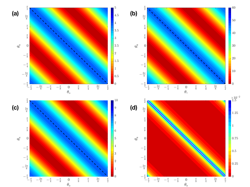
Figure 3: Contour plots of (a) the measurement overlap Eq. (65), (b) the unobserved overlap Eq. (69), (c) the observed overlap Eq. (71) and (d) the RPR for the noisy linear attenuator system in the steady state for different values of the observed (Alice) and unobserved (Bob) homodyne phases. In this example, the range of the unobserved and observed homodyne phases are $\Theta_{\text{u}}=[-\pi/2,\pi/2)$ and $\Theta_{\text{o}}=[-\pi/2,\pi/2)$, respectively. Note that while (a), (b), and (c) look identical, the scales of the contours are very different due to Alice and Bob measuring different channels. In (d) we see that the RPR closely resembles the objective functions in (a)–(c), and the optimal RPR (solid white line), obtained numerically, perfectly matches the maximum of the objective functions. In all plots we consider the case where $\gamma_{\uparrow}=0.999\gamma_{\downarrow}$. Alice perfectly measures the attenuation channel ($\eta_{\downarrow,{\rm o}}=1$, $\theta_{\downarrow,{\rm o}}=\theta_{\text{o}}$), and Bob perfectly measures the amplification channel ($\eta_{\uparrow,{\rm u}}=1$, $\theta_{\downarrow,{\rm u}}=\theta_{\text{u}}$). We have set $\hbar=2$.

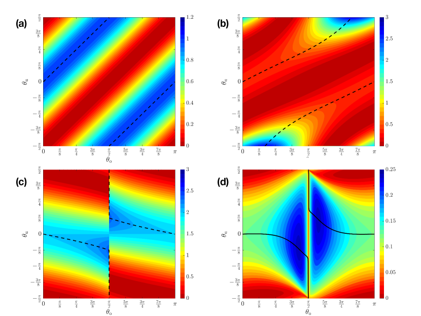
Figure 4: Contour plots of (a) the measurement overlap Eq. (65), (b) the unobserved overlap Eq. (69), (c) the observed overlap Eq. (71) and (d) the RPR for the on-threshold OPO in steady state for different values of the observed (Alice) and unobserved (Bob) homodyne phases. In this example, the range of the unobserved and observed homodyne phases are $\Theta_{\text{u}}=[-\pi/2,\pi/2)$ and $\Theta_{\text{o}}=[0,\pi)$, respectively. In (a), we immediately see that the optimal measurement strategy according to hypothesis A (dashed black line) is very different from the optimal measurement strategy, obtained numerically, for RPR [solid black line in (d)], indicating that it is incorrect. In (b), both the solution to Eq. (70) (dashed black line) and the unobserved overlap behave very differently compared to the optimal measurement strategy and the RPR, respectively, in (d). On the contrary, in (c) the solution to Eq. (66) (dashed black line) gives a close approximation to the optimal measurement strategy. Furthermore, the square overlap has developed some of the characteristics of the RPR. In all plots, both Alice and Bob measure the same damping channel (with homodyne phases $\theta_{\text{o}}$ and $\theta_{\text{u}}$, respectively) but with $\eta_{\text{o}}=\eta_{\text{u}}=0.5$. We have set $\hbar=2$.

VI.1 Hypothesis A

The first and simplest guess at the optimal strategy would be for both Alice and Bob to gather information about the same quantity, e.g., both measuring the same quadrature. Since in the LGQ case the measurement matrices $C_{\text{o}}$ and $C_{\text{u}}$ provide information about how Alice and Bob measure the system, we can look at the overlap between Alice’s and Bob’s measurement matrices,

$${\cal O}_{\rm m}^{\theta_{\text{u}}}(\theta_{\text{o}})=\text{Tr}\left[C_{\text{o}}^{\theta_{\text{o}}}(C_{\text{u}}^{\theta_{\text{u}}})\!^{\top}C_{\text{u}}^{\theta_{\text{u}}}(C_{\text{o}}^{\theta_{\text{o}}})\!^{\top}\right]\,.$$ (65)

Here, for simplicity, we have used the notation $\theta_{\text{o}}$ and $\theta_{\text{u}}$ to denote the parameters specifying Alice’s and Bob’s measurement matrices because in this paper we are restricting to homodyne measurements of a single channel so that only one angle is needed. For the fully general case, we would have to replace $\theta$ by the unraveling matrix $M$ as introduced in Sec. III.2.

It is easiest to see why we call Eq. (65) an overlap function when Alice and Bob only have a single measurement channel at their disposal, like in the OPO example presented in Sec. IV.1. In this case, $C_{\text{o}}$ and $C_{\text{u}}$ become vectors and Eq. (65) is exactly the square of their scalar product. This intuition also works for the noisy linear attenuator example where the only nonzero element in the resulting matrix corresponds to the squared overlap between Alice’s measurement on her channel and Bob’s measurement on his channel. Note that the square is important here, because there is no difference in the information obtained by a measurement with matrix $C$ and one with matrix $-C$, so the objective function ${\cal O}$ should be invariant under a sign change.

Thus, for hypothesis A, that Alice should obtain information about the same quantity as Bob, she choose her measurement by maximizing the measurement overlap function Eq. (65) over the allowed range $\Theta_{\text{o}}$ of homodyne angles. That is, she should choose

$${\color[rgb]{0,0,0}\theta_{\text{o}}^{\star}}(\theta_{\text{u}})=\arg\max_{\theta\in\Theta_{\text{o}}}{\cal O}_{\rm m}^{\theta_{\text{u}}}(\theta)\,,$$ (66)

where we have written Alice’s optimal phase ${\color[rgb]{0,0,0}\theta_{\text{o}}^{\star}}(\theta_{\text{u}})$ as a function of Bob’s homodyne phase. In Eq. (66) we point out that there is no reason to maximize over Alice’s homodyne phase as opposed to Bob’s homodyne phase as the measurement overlap is identical if $C_{\text{o}}$ and $C_{\text{u}}$ are swapped.

We test this intuition by considering the two physical systems presented in Sec. IV in the steady state. For the noisy linear attenuator system, Eq. (66) results in Alice and Bob measuring their respective channels with homodyne phases such that $\theta_{\text{o}}=-\theta_{\text{u}}$. The negative sign arises from the fact that Alice and Bob measure different types of channels, that is, Alice measures an attenuation channel with the Lindblad operator $\sqrt{\gamma_{\downarrow}}(\hat{q}+i\hat{p})$, and Bob measures the amplification channel with the Lindblad operator $\sqrt{\gamma_{\uparrow}}(\hat{q}-i\hat{p})$. Comparing the measurement overlap function in Fig. 3(a) to the RPR in Fig. 3(d), for all $\theta_{\text{o}}=\theta_{\downarrow}$ and $\theta_{\text{u}}=\theta_{\uparrow}$, we see that hypothesis A [dashed black line in (a)] matches perfectly with the optimal measurement strategy [solid white line in (d)] obtained by a numerical search. In fact, the measurement overlap function has a striking resemblance to the RPR for the noisy linear attenuator.

The noisy linear attenuator is, however, a very simple system without any unitary dynamics, so we should not jump to any conclusions about hypothesis A’s success in predicting the optimal measurement. We thus examine the on-threshold OPO system to see how well hypothesis A works. Based on Eq. (66), the optimal measurement strategy for the OPO system is $\theta_{\text{o}}=\theta_{\text{u}}$. This is clearly incorrect, as we can see by comparing the measurement overlap function Fig. 4(a) to the RPR in Fig. 4(d). The numerically obtained optimal strategies [solid black lines in (d)] are drastically different from the hypothesis $\theta_{\text{o}}=\theta_{\text{u}}$ [dashed black lines in (a)]. Furthermore, the measurement overlap function does not resemble the RPR. Consequently, we have to come up with a more refined argument to explain the optimal strategy.

VI.2 Hypothesis B

On reflection, it is perhaps not surprising that hypothesis A failed. Alice’s ultimate goal is to guess Bob’s state as well as possible. Why should that be achieved by trying to get the same type of information as Bob? Rather, it would seem, Alice should try to get information about how Bob’s state changes in reaction to his measurement results, which are unknown to her. That is, it seems that a better hypothesis would take into account the correlation between the measurement setups and the measurement back-action affecting the system.

We can see how a measurement and its corresponding back-action affects the state by comparing the unconditioned equations, Eqs. (20)–(21), to the filtered equations, Eqs. (26)–(27). Specifically, the effect of back-action is given by the kick matrix ${\cal K}^{+}_{\rm r}[V_{\overleftarrow{\rm R}}]$, from which we define a mean-square kick tensor

$$B_{\rm r}^{\theta_{\rm r}}={\cal K}^{+}_{\rm r}[V^{\theta_{\rm r}}_{\overleftarrow{\rm R}}]{\cal K}^{+}_{\rm r}[V^{\theta_{\rm r}}_{\overleftarrow{\rm R}}]^{\top}\,.$$ (67)

Here the superscript $\theta_{\rm r}$ specifies the homodyne phase used to calculate the measurement matrix $C_{\rm r}$, the cross-correlation matrix $\Gamma_{\rm r}$, and the covariance matrix $V_{\overleftarrow{\rm R}}$ (which all feed into ${\cal K}^{+}_{\rm r}[V_{\overleftarrow{\rm R}}]$). The covariance matrix is conditioned on the past measurement record $\overleftarrow{\rm R}=\overleftarrow{\rm O},\overleftarrow{\rm U}$, for ${\rm r}={\rm o},{\rm u}$ respectively. Note that for ${\rm r}={\rm u}$ we are considering the state conditioned only on Bob’s records $\overleftarrow{\color[rgb]{0,0,0}\rm U}$, with a filtered covariance matrix $V^{\theta_{\text{u}}}_{\overleftarrow{\color[rgb]{0,0,0}\rm U}}$ satisfying

$$\frac{{\rm d}V^{\theta_{\text{u}}}_{\overleftarrow{\color[rgb]{0,0,0}\rm U}}}{{\rm d}t}=AV^{\theta_{\text{u}}}_{\overleftarrow{\color[rgb]{0,0,0}\rm U}}+V^{\theta_{\text{u}}}_{\overleftarrow{\color[rgb]{0,0,0}\rm U}}A^{\top}\!+D-{\cal K}_{\text{u}}^{+}[V^{\theta_{\text{u}}}_{\overleftarrow{\color[rgb]{0,0,0}\rm U}}]{\cal K}_{\text{u}}^{+}[V^{\theta_{\text{u}}}_{\overleftarrow{\color[rgb]{0,0,0}\rm U}}]^{\top}\,,$$ (68)

similar to Eq. (27).

As Alice is trying to estimate Bob’s true state of the system, the obvious hypothesis is that Alice should choose her measurement to observe the back-action (kick) Bob’s measurement induces on the system. By choosing this measurement scheme, one would think that Alice’s measurement would contain the most relevant information about Bob’s measurement results and consequently provide a good estimate of the true state. With this in mind, we can construct another objective function, the unobserved overlap function,

$$\color[rgb]{0,0,0}{{\cal O}^{\theta_{\text{u}}}_{\text{u}}(\theta)=\text{Tr}\left[C_{\text{o}}^{\theta}B^{\theta_{\text{u}}}_{\text{u}}(C_{\text{o}}^{\theta})\!^{\top}\right]\,,}$$ (69)

where we have just replaced Bob’s measurement matrix in Eq. (65) with his kick matrix. Thus our hypothesis B is that Alice should choose her measurement in order to maximize the unobserved overlap, i.e.,

$${\color[rgb]{0,0,0}{\color[rgb]{0,0,0}\theta_{\text{o}}^{\star}}(\theta_{\text{u}})=\arg\max_{\theta\in\Theta_{\text{o}}}{\cal O}_{\text{u}}^{\theta_{\text{u}}}(\theta)\,.}$$ (70)

Unsurprisingly, when we consider the noisy linear attenuator example, we see in Fig. 3(b) that the maximum of the unobserved overlap (dashed black line) is obtained when Alice chooses her measurement angle such that $\theta_{\text{o}}=-\theta_{\text{u}}$. However, the same cannot be said for the OPO system, as shown in Fig. 4(b), where both the hypothesized optimal strategy Eq. (70) (dashed black line) and the unobserved overlap function bears little resemblance to the optimal strategy and the RPR in Fig. 4(d), respectively.

VI.3 Hypothesis C

Even though hypothesis B also failed, the construction is still useful. Specifically, we consider the same construction but with Alice and Bob swapped. That is, we consider the counter intuitive hypothesis that it is best for Bob to observe as well as possible the kick from Alice’s measurement on the system. Consequently, we define the observed overlap function

$${\color[rgb]{0,0,0}{\cal O}_{\text{o}}^{\theta_{\text{o}}}(\theta)=\text{Tr}\left[C_{\text{u}}^{\theta}B_{\text{o}}^{\theta_{\text{o}}}(C^{\theta}_{\text{u}})\!^{\top}\right]\,,}$$ (71)

where, compared to Eq. (69), we have swapped the labels ${\rm o}$ and ${\rm u}$. With this overlap function defined, our third and last hypothesis for the optimal unobserved homodyne phase is

$${\color[rgb]{0,0,0}{\color[rgb]{0,0,0}\theta_{\text{u}}^{\star}}(\theta_{\text{o}})=\arg\max_{\theta\in\Theta_{\text{u}}}{\cal O}_{\text{o}}^{\theta_{\text{o}}}(\theta)\,,}$$ (72)

where we have written Bob’s optimal homodyne phase ${\color[rgb]{0,0,0}\theta_{\text{u}}^{\star}}(\theta_{\text{o}})$ as a function of Alice’s homodyne phase and $\Theta_{\text{u}}$ is the range of Bob’s homodyne phase.

Once again, when we consider the noisy linear attenuator, hypothesis C, Eq. (72), still gives the correct optimal solution $\theta_{\text{o}}=-\theta_{\text{u}}$, as can be seen in Fig. 3(c). And this time when we consider the OPO system in Fig. 4(c), we finally do see remarkably good agreement between Eq. (72) (dashed black line) and the optimal measurement strategy [solid black line in Fig. 4(d)]. Furthermore, the objective function for hypothesis C is qualitatively similar to the RPR, with the distinctive asymmetrical peaks close to $\theta_{\text{o}}=\pi/2$ in Fig. 4(d) appearing also in (c).

The above results were for $\eta_{\text{o}}=\eta_{\text{u}}$, but we can also check that hypothesis C can reasonably well predict the optimal measurement strategy for any value of measurement efficiencies. We consider the OPO system, choosing two measurement phases for Alice ($\theta_{\text{o}}=\pi/8$ and $3\pi/8$), and compare the optimal measurement angle for Bob from the hypotheses and from numerics, for all possible observed measurement efficiencies $\eta_{\text{o}}$ with $\eta_{\text{u}}=1-\eta_{\text{o}}$; see Fig. 5. Comparing the numerically optimal measurement strategy (solid black lines) to hypothesis C (dashed red lines), we observe, in both of Alice’s measurement phases, that this hypothesis very well captures the optimal measurement phases $\theta_{\text{u}}$ when Alice’s efficiency is low. At higher efficiencies the agreement in optimal phases (see curves associated with the left axis) is not as perfect. However, when comparing the resulting RPR (curves for the right axis) we observe that the phases given by hypothesis C can still give an RPR extremely close to the maximum value. We can also see how well this approximately optimal solution does compared to another (suboptimal) measurement strategy, hypothesis A (the blue dotted lines), where, especially in the case that $\theta_{\text{o}}=3\pi/8$, the differences in the RPR are much larger.

While hypothesis C seems to provide a good approximation of the optimal strategy; it is not based on any simple physical intuition, unlike hypothesis A and B. However, further evidence that its success here is not a fluke can be gained by applying similar logic to a very different type of quantum system, namely, a qubit.

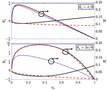
Figure 5: The hypothesized and optimal unobserved measurement phases (left-hand-side axis) and the RPR (right-hand-side axis) for the OPO system in the steady state with varying observed measurement efficiency $\eta_{\text{o}}$ ($\eta_{\text{u}}=1-\eta_{\text{o}}$), for two fixed observed measurement phases (top: $\theta_{\text{o}}=\pi/8$, bottom: $\theta_{\text{o}}=3\pi/8$). We consider two hypotheses of the optimal measurement strategy for Bob, hypothesis A, Eq. (66) (blue dotted line), and hypothesis C, Eq. (72) (red dashed line), comparing to the numerically obtained optimal strategy (black solid line). The results show that the strategy in Eq. (72) gives a very close approximation to the optimal RPR.

VI.4 Qubit Example

The single-qubit example we consider in this section is the same as that presented in Refs. Guevara and Wiseman (2015); Chantasri et al. (2019). The qubit has Hamiltonian $\hat{H}_{0}=\hbar\omega\hat{\sigma}_{z}$ and is coherently driven at frequency $\omega$ and is coupled to a bosonic bath. In a frame that removes $\hat{H}_{0}$, the master equation for the qubit’s unconditioned dynamics is given by

$$\hbar\dot{\rho}=i[(\Omega/2)\hat{\sigma}_{x},\rho]+\gamma{\cal D}[\hat{\sigma}_{-}]\rho\,,$$ (73)

where $(\Omega/2)\hat{\sigma}_{x}$ is the driving Hamiltonian, and $\hat{\sigma}_{-}\equiv(\hat{\sigma}_{x}-i\hat{\sigma}_{y})/2$ is the Lindblad operator. Here $\hat{\sigma}_{k}$ are the standard Pauli matrices. The system-bath coupling rate is denoted by $\gamma$. Alice and Bob could measure the bosonic bath in many different ways Wiseman and Milburn (2010). In this work, we only consider homodyne measurements, as we did for the LGQ systems. The resulting homodyne photocurrent from monitoring the bath is

$$y_{\rm r}{\rm d}t=\sqrt{\gamma\eta}\,C_{\rm r}\langle{{\color[rgb]{0,0,0}\hat{\bf r}}}\rangle_{\overleftarrow{\rm R}}{\rm d}t+{\rm d}w_{\rm r}\,.$$ (74)

Here, $\hat{\bf r}$ is the 3-vector of Pauli operators

$$\hat{\bf r}=\left(\hat{\sigma}_{x},\hat{\sigma}_{y},\hat{\sigma}_{z}\right)^{\top}\,,$$ (75)

whose mean is the Bloch vector, which represents the quantum state. In Eq. (74), this mean is conditioned on the past record $\overleftarrow{\rm R}=\overleftarrow{\color[rgb]{0,0,0}\rm O},\overleftarrow{\color[rgb]{0,0,0}\rm U}$ corresponding to $\rm r=\rm o,\rm u$ respectively. As before, $\eta$ is the measurement efficiency and the qubit analogue of measurement matrix is

$$C_{\rm r}=[\cos(\theta_{\rm r}),\sin(\theta_{\rm r}),0]$$ (76)

for this particular example.

We will restrict our analysis to two cases for the measurement: $x$ homodyne and $y$ homodyne, i.e., $\theta_{\rm r}=0$ and $\theta_{\rm r}=\pi/2$, respectively. These choices are the natural ones given the symmetries of Eq. (73). These are named $x$ and $y$ homodyne because of the corresponding Pauli operator appearing in the mean photocurrent signal, from Eq. (76). These two cases best illuminate the effect of measurement choices on the relative average purity recovery in the limit of large $\Omega$. Here we choose $\Omega=5\gamma$. We will also assume that Alice and Bob monitor this bath with equal measurement efficiencies, i.e., $\eta_{\text{o}}=\eta_{\text{u}}=1/2$. We follow the analysis of the qubit’s relative average purity recovery presented in Ref. Chantasri et al. (2019), using numerical analyses, because there is no closed- form solution for the qubit case.

By numerically generating a large ensemble of measurement records and qubit trajectories (including true states, filtered states, and smoothed states) as functions of time, we can calculate the purity recovery averaged over the observed records as in Eq. (63). Since we are interested in the steady-state regime, we need to consider the time period in the simulation to study the qubit’s dynamics independently of the transient effects at the start and end of the interval. Using the dephasing time defined as $T_{\gamma}=1/\gamma$ and the final time $T=8T_{\gamma}$, we choose the steady-state period to be $\mathfrak{T}_{\rm ss}=[4.5T_{\gamma},6T_{\gamma}]$. We show in Fig. 6(d), the $2\times 2$ table of the relative average purity recovery averaged over the steady-state period quoted from Ref. Chantasri et al. (2019), considering four options of Alice’s (O) and Bob’s (U) measurements. The combination with the best performance is when Alice and Bob measure the same quadrature and the worst performance when Alice measures the $y$ quadrature and Bob measures the $x$ quadrature. Thus we next ask whether hypothesis A, B, or C can correctly predict all features of the relative average purity recovery.

As we have already defined the measurement matrix for this qubit example, $C_{\rm r}$ in Eq. (74), the measurement overlap and optimal measurement strategy for hypothesis A are as defined in Eq. (65) and (66), respectively. As we are only considering two measurement possibilities for Alice and Bob, the maximization over the range of the unobserved homodyne phases can be replaced by maximizing over the set $\Theta_{\text{o}}=\{0,\pi/2\}$. Calculating the measurement overlap for the four possible measurement combinations for Alice and Bob, we see, in Fig. 6(a), that the optimal measurement strategy, according to hypothesis A, occurs when Alice and Bob choose the same measurement. This is consistent with the greatest improvement in the average purity of the smoothed state, as seen in Fig. 6(d). However, in the cases where Alice and Bob choose different measurements, we see that the measurement overlap function suggest that there is no difference between these last two cases, which clearly is not true when we look at the relative average purity recovery. Once again, hypothesis A is not very accurate.

To analyze hypotheses B and C for the qubit case, we need to define a quantity that resembles the mean-square kick tensor of the LGQ system. The kick matrix is defined in Eqs. (26) and (37) and describes the measurement back-action for an LGQ system in terms of the change in the system’s expectation values in the $q$ and $p$ quadratures. Given a measurement setting $\rm r\in\{\rm o,\rm u\}$ and its corresponding measurement record $\overleftarrow{\color[rgb]{0,0,0}\rm R}\in\{\overleftarrow{\color[rgb]{0,0,0}\rm O},\overleftarrow{\color[rgb]{0,0,0}\rm U}\}$, respectively, we can rewrite the mean- square kick tensor as

$${\color[rgb]{0,0,0}B_{\rm r}}{\rm d}t={\cal K}^{+}_{\rm r}[V_{\overleftarrow{\color[rgb]{0,0,0}\rm R}}]{\cal K}^{+}_{\rm r}[V_{\overleftarrow{\color[rgb]{0,0,0}\rm R}}]^{\top}{\rm d}t=\mathbb{E}_{\overleftarrow{\color[rgb]{0,0,0}\rm R}}\left[{\rm d}\langle{\hat{\bf x}}\rangle_{\overleftarrow{\color[rgb]{0,0,0}\rm R}}{\rm d}{\langle{\hat{\bf x}}\rangle^{\top}_{\overleftarrow{\color[rgb]{0,0,0}\rm R}}}\right].$$ (77)

Here $\langle{\hat{\bf x}}\rangle_{\overleftarrow{\color[rgb]{0,0,0}\rm R}}$ is the LGQ phase-space mean conditioned on a realization of the (past) record $\overleftarrow{\color[rgb]{0,0,0}\rm R}$, and the expected average on the right-hand side of Eq. (77) is over all possible record realizations. The right-hand side is exactly the mean-square change (during an infinitesimal time ${\rm d}t$) of the system’s expectation values, in a tensorial sense, averaging over all the possible records. Therefore we can define an analogous quantity to the mean-square kick tensor for the qubit system as

$$\begin{split}{\color[rgb]{0,0,0}B_{\rm r}}=\mathbb{E}_{\overleftarrow{\color[rgb]{0,0,0}\rm R}}\left\{\frac{1}{|\mathfrak{T}_{\rm ss}|}\,\!\!\sum_{t\in\mathfrak{T}_{\rm ss}}\left[{\rm d}\langle{{\color[rgb]{0,0,0}\hat{\bf r}}}\rangle_{\overleftarrow{\rm R}}(t)\,{\rm d}\langle{{\color[rgb]{0,0,0}\hat{\bf r}}}\rangle_{\overleftarrow{\rm R}}(t)^{\top}\right]\right\}\,,\end{split}$$ (78)

for the steady-state period $\mathfrak{T}_{\rm ss}$ of length $|\mathfrak{T}_{\rm ss}|$.

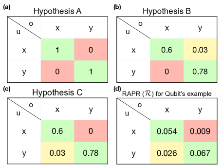
Figure 6: Analysis of hypothesis A, B, and C and the relative average purity recovery (${\cal R}$) for the example of a driven qubit coupled dissipatively to a bosonic bath. We restrict Alice and Bob to only two measurement choices, either $x$ or $y$ homodyne. The numerical values in tables (a), (b), and (c) are the objective functions for the respective hypotheses. For B and C this required stochastic simulated, and we used 3000 records each. The qubit’s relative average purity recovery [Table (d)] is obtained using the numerical techniques presented in Ref. Chantasri et al. (2019), simulating $3000$ observed and $10000$ unobserved records for both measurement settings. Here the coloured cells indicate good (green), moderate (yellow), and bad (red) improvement. Only hypothesis C [Table (c)] correctly predicts the pattern of the relative average purity recovery.

Now that we have defined the mean-square kick tensor for the qubit setting, we can formalize and analyze both hypothesis B and C. We will begin with hypothesis B, where the unobserved overlap and optimal measurement strategy are as defined in Eqs. (69)–(70), where, as in hypothesis A, we maximize over the set $\Theta_{\text{o}}=\{0,\pi/2\}$. As seen from the four possible measurement combinations for Alice and Bob in Fig. 6(b), the optimal measurement choice for Alice, according to Eq. (70), occurs when Alice and Bob choose the same measurement, and best of all is when both choose homodyne measurements along the $y$ direction. This is consistent with the actual relative average purity recovery, as seen in Fig. 6(d). However, when we investigate the other measurement combinations, specifically when Alice and Bob choose different measurements, we see that the unobserved overlap function does not reproduce the pattern seen for the relative average purity recovery. That is, it predicts that smoothing would be better if Alice chose $y$ and Bob $x$ rather than the other way around, whereas the truth is the opposite.

For hypothesis C, the roles of Alice and Bob are reversed compared to hypothesis B, and the optimal measurement for Bob is given by Eq. (72) and the observed overlap defined in Eq. (71). As was the case for hypothesis B, we are restricting our analysis to two measurement choices for Alice and Bob, and the maximization is instead over the set $\Theta_{\text{u}}=\{0,\pi/2\}$. For the four possible measurement choices for Alice and Bob, shown in Fig. 6(c), the best combination is when both measure $y$ and the second best when both measure $x$, consistent with the relative average purity recovery, Fig. 6(d), and the same as in hypothesis B. However, unlike for hypothesis B, this time the objective function for the cases when Alice and Bob choose different measurements also matches the relative average purity recovery. This shows that hypothesis C is better at predicting when smoothing will work well than either hypothesis A or hypothesis B. This is consistent with the results obtained for the LGQ systems.

VII Conclusion

In this paper we provided a detailed derivation of the smoothed quantum state for LGQ systems and contrasted it with the theory of the smoothed weak-value state. To exemplify the differences between these techniques, we simulated a single trajectory and witnessed clear differences in the dynamics of the estimates by looking at the filtered, the SWV state, and the smoothed quantum states for LGQ systems. As expected, the last of these provides the best estimate of the true state conditioned on the results of measurements on a channel unavailable to the observer, Alice, as well as on the results of Alice’s measurements.

A key question of interest is how much improvement smoothing can offer relative to filtering and how this depends on the measurement choices of Alice and Bob (the observer of the channel unavailable to Alice). We studied this through the purity recovery of smoothing over filtering relative to the maximum possible purity recovery. We constructed three different hypotheses about what properties of Alice and Bob’s measurements would lead to higher relative purity recovery.

We found that the only hypothesis that worked, qualitatively, for the two LQG systems we studied is the most counter intuitive of the three. It is the hypothesis that says Bob should choose his measurement so that his signal tells him as much as possible about the disturbance to the state caused by Alice’s measurements. This is counter intuitive because one would have thought that it is Alice, the one doing the smoothing, who needs to be able to infer as accurately as possible the disturbance to the state caused by Bob’s measurement. After all, it is the existence of this disturbance that makes Alice’s filtered state impure and allows the possibility of increasing the purity by smoothing.

The qualitative success of our third hypothesis is the main result of this paper. However, it presents a puzzle because it is not grounded in physical intuition. For this reason we also put our three hypotheses to the test on a very different system, specifically, a qubit system, not an LGQ system. We formulated the problem in a closely analogous way to that used for LGQ systems and found that, once again, our third hypothesis was clearly superior to the other two in predicting which combinations of measurements by Alice and Bob would give better relative purity recovery than the other combinations.

It can be hoped that further study will elucidate why it is preferable for Bob to measure the system so as to detect the ‘kick’ to the state by Alice’s measurement, rather than the converse. Another interesting question is what would happen to the smoothed state if Alice were to assume the incorrect type of measurement for Bob. Could the smoothed state be a worse estimate of the true state than the filtered state? The LGQ formalism offers a convenient way to explore this because of the possibility of semianalytic solutions. There is also a great deal of work to be done in comparing the various other ways of utilising past and future measurement information, such as the most likely path formalism Chantasri et al. (2013); Weber et al. (2014), and in applying these theories to the LGQ scenario.