Quantum random access memory via quantum walk

Abstract

A novel concept of quantum random access memory (qRAM) employing a quantum walk is provided. Our qRAM relies on a bucket brigade scheme to access the memory cells. Introducing a bucket with chirality left and right as a quantum walker, and considering its quantum motion on a full binary tree, we can efficiently deliver the bucket to the designated memory cells, and fill the bucket with the desired information in the form of quantum superposition states. Our procedure has several advantages. First, we do not need to place any quantum devices at the nodes of the binary tree, and hence in our qRAM architecture, the cost to maintain the coherence can be significantly reduced. Second, our scheme is fully parallelized. Consequently, only $O(n)$ steps are required to access and retrieve $O(2^{n})$ data in the form of quantum superposition states. Finally, the simplicity of our procedure may allow the design of qRAM with simpler structures.

1 Introduction

The development of an efficient procedure to retrieve classical/quantum data from a database and transform them into a quantum superposition state is one of the most fundamental issues for a practical realization of quantum information processing. Quantum random access memory (qRAM) that stores information and permits queries in superposition may play a pivotal role in a substantial speedup of quantum algorithms for data analysis [1, 2, 3], including applications to machine learning for big data [4, 5, 6, 7, 8].

qRAM is a quantum analog of classical RAM. Provided a superposition of addresses $\sum_{a}|a\rangle$ ($a\in\mathbb{Z}_{\geq 0}$) as input, qRAM accesses the $a$th cell in the memory array, where classical information $|x^{(a)}\rangle$ is stored, and outputs a superposition of $|x^{(a)}\rangle$’s correlated with the addresses. Note here that qRAM is possible to store either classical information (i.e. each $|x^{(a)}\rangle$ does not consist of any superposition of states) or quantum information(i.e. each $|x^{(a)}\rangle$ is an arbitrary superposition of states). In this paper, we restrict ourselves to the classical case, and assume that the addresses $|a\rangle$ and the data $|x^{(a)}\rangle$ ($a,x^{(a)}\in\mathbb{Z}_{\geq 0}$) consist of $n$ and $m$ qubits, respectively.

More precisely, qRAM is defined as

$$\text{qRAM}:\,\, \sum_{a}|a\rangle_{A}|0\rangle_{D}\mapsto\sum_{a}|a\rangle_{A}|x^{(a)}\rangle_{D},$$

$$|a\rangle_{A}\in\mathbb{C}^{2n},\,\,|x^{(a)}\rangle_{D}\in\mathbb{C}^{2m}\quad(n,m\in\mathbb{Z}_{\geq 0}).$$ (1.1)

where $A$ and $D$, respectively, denote quantum analogs of an address register (input register) and a data register (output register). Namely, qRAM (1.1) is a quantum device consisting of (i) a routing scheme to access the designated memory cells, (ii) a querying scheme to retrieve the data stored in the cells, and (iii) an output scheme to encode the data into a superposition of quantum states.

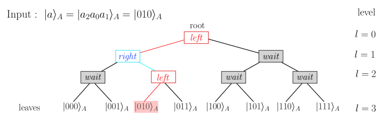
Figure 1: A bucket brigade scheme on the full binary tree with depth $n=3$. The qutrits are equipped at each node. To route to the memory cell $|010\rangle_{A}$, one must activate the three qutrits as in the figure.

As a quantum routing scheme, a notable idea, the “bucket brigade” scheme has been proposed by Giovannetti, Lloyd and Maccone (GLM) [9, 10] to overcome difficulties associated with the conventional fanout scheme commonly implemented in classical RAM (see [11, 12], for instance). The bucket brigade architecture employs a perfect binary tree with $O(N)$ ($N=2^{n}$) nodes routing a signal from the root down to one of the $N$ leaves interpreted as the memory cells (see Fig. 1 for $n=3$.). Let $|a_{n-1}\cdots a_{0}\rangle$ ($a_{l}\in\{0,1\}$; $0\leq l\leq n-1$) be the binary representation of the address of the cell. The value of $a_{l}$ indicates the route from a parent node at the $l$th level to one of the two children nodes at the $(l+1)$th level. For instance, the left (resp. right) child is chosen if $a_{l}=0$ (resp. $a_{l}=1$). In consequence, each of the $N$ possible values of the address register uniquely determines a path in the binary tree.

In the original GLM architecture, a qutrit (i.e. a three-level quantum system with energy levels labeled by wait, left and right) is allocated at each node, and all the qutrits are initialized to be wait state. The value $a_{l}$ is sequentially delivered from the root to a node at the $l$th level, and activates the qutrit to left (right) if $a_{l}=0$ ($a_{l}=1$) to route the following $a_{l+1}$ to one of the two subsequent nodes. After $O(n^{2})$ time steps, a unique path from the root to the designated memory cell is assigned as depicted in Fig 1 for $n=3$ and $|a\rangle_{A}=|010\rangle_{A}$. Remarkably, only $n$ qutrits are activated, which is exponentially less than that for the traditional fanout architecture, where $N$ quantum switches are necessary to be activated. Namely, the GLM bucket brigade architecture has a significant advantage in maintaining quantum coherence.

A quantum signal (the so-called quantum bus) can follow the path to the desired memory cell through the activated qutrits, retrieve information stored in the cell, and goes back to the root along the path. Finally, resetting the activated qutrits to be the initialized state wait one by one starting from the last level of the tree, one obtains the output as in the r.h.s. of (1.1). That is the GLM bucket brigade qRAM. The GLM scheme has been improved, and concretely implemented into quantum circuits as in [13, 14, 15, 16]. (Note that a different concept of qRAM without relying on any routing schemes has recently been developed in [17].)

This paper provides a novel concept of qRAM, which employs a discrete-time quantum walk as a bucket brigade scheme. A quantum walk is a quantum motion of a particle (interpreted as a bucket) possessing chirality left and right [18, 19]. The quantum bucket with chirality left (resp. right) on a parent node moves to the left (resp. right) child node. Each scheme of qRAM can actually be realized by quantum motions of multiple quantum walkers. Our procedure has several advantages. First, because we do not need to equip any quantum devices at the totally $O(n2^{n})$ nodes on the binary tree, the cost to maintain the coherence can be reduced. Consequently, our qRAM may be much more robust against the decoherence arising from noises at the nodes. Second, each procedure is fully parallelized. As a result, only $O(n)$ steps are required to access and retrieve data in the form of quantum superposition states. Finally, since the three schemes required in qRAM are entirely independent of each other, the architecture of qRAM can be simplified.

The layout of this paper is as follows. In the subsequent section, we introduce a quantum walk on a binary tree. qRAM utilizing the quantum walk is constructed in Sec. 3. In Sec. 4, we give some specific examples of how to implement our qRAM scheme using multiple quantum walkers. The last section is devoted to a summary.

2 Quantum walk on a binary tree

Quantum walks, which are the quantum counterparts of classical random walks, are defined as a class of unitary time-evolutions on graphs. In contrast to the classical random walks, the randomness comes from a superposition of quantum states and its time evolution. Here, let us introduce a discrete-time quantum walk on a full binary tree. A quantum particle with chirality $|0\rangle_{C}$ (left) and $|1\rangle_{C}$ (right) may be interpreted as a quantum “bucket”. A bucket with chirality $|0\rangle_{C}$ (resp. $|1\rangle_{C}$) deviates left (resp. right) at each node of the binary tree, which is in contrast to a bucket in the GLM architecture, where the route is determined by activating the qutrit equipped at each node (see the previous section). In consequence, we do not need to equip any quantum devices at the $O(n2^{n})$ nodes, which is one of the main advantages in our scheme.

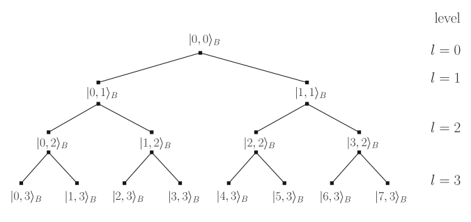
Figure 2: A full binary tree with depth $n=3$. The state $|w,l\rangle_{B}$ ($0\leq w\leq 2^{l}-1$, $0\leq l\leq n$) denotes the position of the $w$th node counting from the left in level $l$.

We consider the full binary tree with depth $n$ (i.e. it has totally $2^{n}$ leaves corresponding to the memory cells) (see Fig. 2 for $n=3$). Let $|w,l\rangle_{B}$ denote the position of the $w$th node counting from the left in level $l$ ($0\leq w\leq 2^{l}-1$, $0\leq l\leq n$). We call $V_{B}=\bigoplus_{w,l}V_{(w,l)}$ ($V_{(w,l)}=\mathbb{C}$) spanned by $|w,l\rangle_{B}$ ($0\leq w\leq 2^{l}-1$, $0\leq l\leq n$) and $V_{C}=\mathbb{C}^{2}$ spanned by $|c\rangle_{C}$ ($c\in\{0,1\}$) “bus space” and “chirality space”, respectively. The quantum walk is defined on the space $V_{B}\otimes V_{C}$. The quantum walker at the node $|w,l\rangle_{B}$ moves to the left (resp. right) child node $|2w,l+1\rangle_{B}$ (resp. $|2w+1,l+1\rangle_{B}$) when the chirality of the walker is $|0\rangle_{C}$ (resp. $|1\rangle_{C}$). This can be represented by the operator $\mathcal{S}_{(w,l)}$ acting on the space $(V_{(w,l)}\oplus V_{(2w,l+1)}\oplus V_{(2w+1,l+1)})\otimes V_{C}=\mathbb{C}^{6}$:

$$\mathcal{S}_{(w,l)}:\,\,|w,l\rangle_{B}|0\rangle_{C}\mapsto|2w,l+1\rangle_{B}|0\rangle_{C},$$

$$\mathcal{S}_{(w,l)}:\,\,|w,l\rangle_{B}|1\rangle_{C}\mapsto|2w+1,l+1\rangle_{B}|1\rangle_{C}.$$ (2.1)

In addition, the walker at the left (resp. right) child node $|2w,l+1\rangle_{B}$ (resp. $|2w+1,l+1\rangle_{B}$) can be pulled back to the parent node $|w,l\rangle_{B}$ by $\mathcal{S}_{(w,l)}$ only if its chirality is $|0\rangle_{C}$ (resp. $|1\rangle_{C}$), and stays at the present position if its chirality is $|1\rangle_{C}$ (resp. $|0\rangle_{C}$). Explicitly,

$$\mathcal{S}_{(w,l)}:\,\,|2w,l+1\rangle_{B}|0\rangle_{C}\mapsto|w,l\rangle_{B}|0\rangle_{C},$$

$$\mathcal{S}_{(w,l)}:\,\,|2w+1,l+1\rangle_{B}|1\rangle_{C}\mapsto|w,l\rangle_{B}|1\rangle_{C},$$

$$\mathcal{S}_{(w,l)}:\,\,|2w,l+1\rangle_{B}|1\rangle_{C}\mapsto|2w,l+1\rangle_{B}|1\rangle_{C},$$

$$\mathcal{S}_{(w,l)}:\,\,|2w+1,l+1\rangle_{B}|0\rangle_{C}\mapsto|2w+1,l+1\rangle_{B}|0\rangle_{C}.$$ (2.2)

Namely, $\mathcal{S}_{(w,l)}\in\mathrm{End}((V_{(w,l)}\oplus V_{(2w,l+1)}\oplus V_{(2w+1,l+1)})\otimes V_{C})$ is a unitary operator expressed as

$$\mathcal{S}_{(w,l)}= \sum_{i=0}^{1}\Bigl{(}\left|2w+i,l+1\right\rangle\left\langle w,l\right|+\left|w,l\right\rangle\left\langle 2w+i,l+1\right|\Bigr{)}_{B}\otimes|i\rangle\langle i|_{C}$$

$$+\sum_{i=0}^{1}\left|2w+\frac{1+(-1)^{i}}{2},l+1\right\rangle\left\langle 2w+\frac{1+(-1)^{i}}{2},l+1\right|_{B}\otimes\left|i\right\rangle\left\langle i\right|_{C}.$$ (2.3)

Combining a unitary operator $\mathcal{C}$ acting on $V_{C}$, we obtain a non-trivial quantum motion on the graph. In the next section, we construct $\mathcal{C}$ such that it acts on both $V_{C}$ and the “address space” $V_{A}=({\mathbb{C}^{2}})^{\otimes n}$ to move the quantum walker (bucket) from the root to a specific leaf (memory cell) and to return the bucket filled with information back to the original root.

3 qRAM via quantum walk

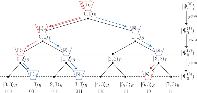
Figure 3: A pictorial example of the routing scheme (3.7) for the case that $n=3$ and the input addresses are $\sum|a\rangle_{A}=|001\rangle_{A}+|011\rangle_{A}+|110\rangle_{A}$. Namely, the initial state is given by $|\Phi_{0}^{(0)}\rangle=\sum_{a}|0,0\rangle_{B}|0\rangle_{C}|a\rangle_{A}|0\rangle_{D}$, and depicted as the red bucket (in quantum superposition) located at the node $|0,0\rangle_{B}$. Red corresponds to the chirality $|0\rangle_{C}$ and blue to $|1\rangle_{C}$. Operating $\mathcal{F}^{(1|0)}$ defined by (3.8) on $|\Phi_{0}^{(0)}\rangle$, one has $|\Phi_{0}^{(1)}\rangle=|0,1\rangle_{B}|0\rangle_{C}(|001\rangle_{A}+|011\rangle_{A})|0\rangle_{D}+|1,1\rangle_{B}|1\rangle_{C}|110\rangle_{A}|0\rangle_{D}$. Similarly, $\mathcal{F}^{(2|1)}|\Phi_{0}^{(1)}\rangle$ yields $|\Phi_{0}^{(2)}\rangle=|0,2\rangle_{B}|0\rangle_{C}|001\rangle_{A}|0\rangle_{D}+|1,2\rangle_{B}|1\rangle_{C}|011\rangle_{A}|0\rangle_{D}+|3,2\rangle_{B}|1\rangle_{C}|110\rangle_{A}|0\rangle_{D}.$ Finally, $\mathcal{F}^{(3|2)}|\Phi^{(2)}_{0}\rangle$ reads $\Phi^{(3)}=|1,3\rangle_{B}|1\rangle_{C}|001\rangle_{A}|0\rangle_{D}+|3,3\rangle_{B}|1\rangle_{C}|011\rangle_{A}|0\rangle_{D}+|6,3\rangle_{B}|0\rangle_{C}|110\rangle_{A}|0\rangle_{D}$. Thus, one can deliver the bucket in superposition to the designated addresses $\sum|a\rangle_{A}$.

To appropriately access and retrieve data stored in the specified memory cells in the form of quantum superposition, we employ the quantum walk explained in the previous section. Let

$$|x^{(a)}\rangle_{D}=|x^{(a)}_{m-1}\cdots x^{(a)}_{0}\rangle_{D}=|x^{(a)}_{m-1}\rangle_{D_{m-1}}\cdots|x^{(a)}_{0}\rangle_{D_{0}}\quad(x^{(a)}_{i}\in\{0,1\};\,0\leq i\leq m-1),$$

$$|x^{(a)}_{i}\rangle\in V_{D_{i}}=\mathbb{C}^{2},\quad|x^{(a)}\rangle_{D}\in V_{D}=\bigotimes_{i=0}^{m-1}V_{D_{i}}=(\mathbb{C}^{2})^{\otimes m}$$ (3.1)

be the binary representation of data stored in a memory cell. Here, $|a\rangle_{A}$ ($0\leq a\leq N-1$; $N=2^{n}$) represents the address of the cell:

$$|a\rangle_{A}=|a_{n-1}\cdots a_{0}\rangle_{A}=|a_{n-1}\rangle_{A_{n-1}}\cdots|a_{0}\rangle_{A_{0}}\quad(a_{i}\in\{0,1\};\,0\leq i\leq n-1),$$

$$|a_{i}\rangle\in V_{A_{i}}=\mathbb{C}^{2},\quad|a\rangle_{A}\in V_{A}=\bigotimes_{i=0}^{n-1}V_{A_{i}}=(\mathbb{C}^{2})^{\otimes n}.$$ (3.2)

Let us call $V_{A}$ and $V_{D}$ the “address space” and the “data space”, respectively. Our qRAM is defined on the space

$$V:=V_{B}\otimes V_{C}\otimes V_{A}\otimes V_{D}$$ (3.3)

as

$$\text{qRAM}:\,\,\sum_{a\in\mathscr{A}}|0,0\rangle_{B}|0\rangle_{C}|a\rangle_{A}|0\rangle_{D}\mapsto\sum_{a\in\mathscr{A}}|0,0\rangle_{B}|0\rangle_{C}|a\rangle_{A}|x^{(a)}\rangle_{D},$$ (3.4)

where $\mathscr{A}\subset\{0,1,\cdots,N-1\}$.

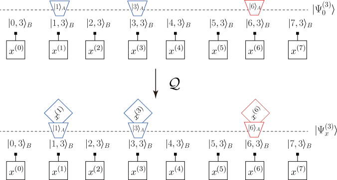
Figure 4: A pictorial example of the querying scheme (3.12) and (3.13) for the empty bucket (in quantum superposition) delivered at the memory cells addressed by $\sum|a\rangle_{A}=|001\rangle_{A}+|011\rangle_{A}+|110\rangle_{A}$ (see Fig. 3 for $|\Phi^{(3)}_{0}\rangle$). Performing $\mathcal{Q}$ on the state $|\Phi^{(3)}_{0}\rangle$, one obtains $|\Phi^{(3)}_{x}\rangle=|1,3\rangle_{B}|1\rangle_{C}|001\rangle_{A}|x^{(1)}\rangle_{D}+|3,3\rangle_{B}|1\rangle_{C}|011\rangle_{A}|x^{(3)}\rangle_{D}+|6,3\rangle_{B}|0\rangle_{C}|110\rangle_{A}|x^{(6)}\rangle_{D}$ which denotes the bucket filled with the data.

As described in Sec. 1, qRAM consists of the following three schemes: (i) a routing scheme to move the empty bucket in a superposition to specific cells, (ii) a querying scheme to fill the bucket with data and (iii) an output scheme to pull back the bucket and output the data in the form of quantum superposition states. Correspondingly, the qRAM is decomposed into the following three operators:

$$\text{qRAM}=\mathcal{F}^{\dagger}\mathcal{Q}\mathcal{F}\in\mathrm{End}(V).$$ (3.5)

(i) Routing scheme. First we construct the routing scheme $\mathcal{F}\in\mathrm{End}(V_{A}\otimes V_{B}\otimes V_{C})$. Let $|\Psi_{0}^{(l)}\rangle\in V$ be a state that the bucket in a superposition is located at nodes in level $l$ (see Fig. 3 as an example). We set

$$|\Psi_{0}^{(0)}\rangle=\sum_{a\in\mathscr{A}}|0,0\rangle_{B}|0\rangle_{C}|a\rangle_{A}|0\rangle_{D}$$ (3.6)

as the initial state. One finds that the bucket in a superposition is appropriately delivered to the desired cells at $\sum_{a\in\mathscr{A}}|a\rangle_{A}$ by $\mathcal{F}$:

$$\mathcal{F}:\,\,|\Psi_{0}^{(0)}\rangle\mapsto|\Psi_{0}^{(n)}\rangle,$$ (3.7)

which is decomposed into $\mathcal{F}=\mathcal{F}^{(n|n-1)}\cdots\mathcal{F}^{(1|0)},$ where the element $\mathcal{F}^{(l+1|l)}$

$$\mathcal{F}^{(l+1|l)}:\,\,|\Psi_{0}^{(l)}\rangle\mapsto|\Psi_{0}^{(l+1)}\rangle,\quad|\Psi_{0}^{(l)}\rangle:=\left|\sum_{k=1}^{l}2^{l-k}a_{n-k},l\right\rangle_{B}|a_{n-l}\rangle_{C}|a\rangle_{A}|0\rangle_{D}$$ (3.8)

is given by

$$\mathcal{F}^{(l+1|l)}:=\sum_{w=0}^{2^{l}-1}\mathcal{S}_{(w,l)}\mathcal{C}_{C,A_{n-(l+1)}}\mathcal{C}_{C,A_{n-l}}.$$ (3.9)

Here, $\mathcal{S}_{(w,l)}$ is the shift operator defined by (2.3) (see also (2.1) and (2.2)) and $\mathcal{C}_{C,{A_{l}}}\in\mathrm{End}(V_{C}\otimes V_{A_{l}})$ is so-called the controlled NOT operator defined as

$$\mathcal{C}_{C,A_{l}}:=I_{C}\otimes|0\rangle\langle 0|_{A_{l}}+X_{C}\otimes|1\rangle\langle 1|_{A_{l}},\quad\mathcal{C}_{C,A_{n}}:=I_{C},$$ (3.10)

where $X_{C},I_{C}\in\mathrm{End}(V_{C})$ are, respectively, the Pauli $X$ operator and the identity matrix. Eq. (3.8) can be recursively derived as follows:

$$|\Psi_{0}^{(0)}\rangle=\sum_{a\in\mathscr{A}}|0,0\rangle_{B}|0\rangle_{C}|a\rangle_{A}|0\rangle_{D}\xrightarrow{\mathcal{F}^{(1|0)}=\mathcal{S}_{(0,0)}\mathcal{C}_{C,A_{n-1}}\mathcal{C}_{C,A_{n}}}$$

$$|\Psi_{0}^{(1)}\rangle=\sum_{a\in\mathscr{A}}|a_{n-1},1\rangle_{B}|a_{n-1}\rangle_{C}|a\rangle_{A}|0\rangle_{D}\xrightarrow{\mathcal{F}^{(2|1)}=(\mathcal{S}_{(0,1)}+\mathcal{S}_{(1,1)})\mathcal{C}_{C,A_{n-2}}\mathcal{C}_{C,A_{n-1}}}$$

$$|\Psi_{0}^{(2)}\rangle=\sum_{a\in\mathscr{A}}|2a_{n-1}+a_{n-2},2\rangle_{B}|a_{n-2}\rangle_{C}|a\rangle_{A}|0\rangle_{D}\cdots\xrightarrow{\mathcal{F}^{(l|l-1)}=\sum_{w=0}^{2^{l-1}-1}\mathcal{S}_{(w,l-1)}\mathcal{C}_{C,A_{n-l}}\mathcal{C}_{C,A_{n-(l-1)}}}$$

$$|\Psi_{0}^{(l)}\rangle=\sum_{a\in\mathscr{A}}\left|\sum_{k=1}^{l}2^{l-k}a_{n-k},l\right\rangle_{B}|a_{n-l}\rangle_{C}|a\rangle_{A}|0\rangle_{D}\cdots\xrightarrow{\mathcal{F}^{(n|n-1)}=\sum_{w=0}^{2^{n-1}-1}\mathcal{S}_{(w,n-1)}\mathcal{C}_{C,A_{0}}\mathcal{C}_{C,A_{1}}}$$

$$|\Psi_{0}^{(n)}\rangle=\sum_{a\in\mathscr{A}}|a,n\rangle_{B}|a_{0}\rangle_{C}|a\rangle_{A}|0\rangle_{D}.$$ (3.11)

Note that, in the last step, we have used $a=\sum_{k=1}^{n}2^{n-k}a_{n-k}$. As the result, the bucket in a superposition state is delivered to the desired memory cells located at $\sum_{a\in\mathscr{A}}|a\rangle$. In Fig. 3, we pictorially show the routing scheme. One easily sees that $O(n)$ steps are required for the routing scheme.

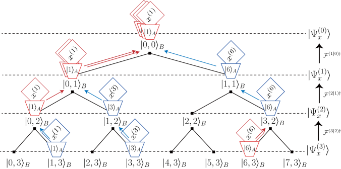
Figure 5: A pictorial example of the output scheme (3.14). Due to the unitarity of $\mathcal{F}$ (3.7), the bucket filled with the data (see Figs. 3 and 4) can be pulled back to the root in the opposite procedure as the routing scheme: $|\Phi^{(0)}_{x}\rangle=\mathcal{F}^{\dagger}|\Phi^{(3)}_{x}\rangle=\sum_{a}|0,0\rangle_{B}|0\rangle_{C}|a\rangle_{A}|x^{(a)}\rangle$.

(ii) Querying scheme. Since our schemes are independent of each other, the querying scheme $\mathcal{Q}\in\mathrm{End}(V_{B}\otimes V_{D})$ to retrieve information from the memory cells can be significantly simplified and easily parallelized. The operator $\mathcal{Q}$ defined as

$$\mathcal{Q}:\,\,|\Psi_{0}^{(n)}\rangle\mapsto|\Psi_{x}^{(n)}\rangle,\quad|\Psi_{x}^{(n)}\rangle:=\sum_{a\in\mathscr{A}}|a,n\rangle_{B}|a_{0}\rangle_{C}|a\rangle_{A}|x^{(a)}\rangle_{D}$$ (3.12)

can be simply composed by the Pauli $X$ operator $X_{D_{i}}\in\mathrm{End}(V_{D_{i}})$:

$$\mathcal{Q}:=\sum_{a=0}^{2^{n}-1}|a,n\rangle\langle a,n|_{B}\otimes\left[\bigotimes_{i=0}^{m-1}\left(X_{D_{i}}\right)^{x_{i}^{(a)}}\right].$$ (3.13)

The querying scheme is shown in Fig. 4. Note that the time steps necessary for the querying scheme is only $O(1)$.

(iii) Output scheme. Due to the unitarity of the operators (see (2.2) and (3.10)), one easily finds that the quantum walk is reversible. Namely, the output scheme to pull back the bucket filled with the data can be achieved in exactly the opposite manner as the routing scheme:

$$\mathcal{F}^{\dagger}:\,\,|\Psi_{x}^{(n)}\rangle\mapsto|\Psi_{x}^{(0)}\rangle,\quad|\Psi_{x}^{(0)}\rangle:=\sum_{a\in\mathscr{A}}|0,0\rangle_{B}|0\rangle_{C}|a\rangle_{A}|x^{(a)}\rangle_{D}.$$ (3.14)

See Fig. 5 as an example of the output scheme.

Thus, we find that our qRAM (3.5) satisfies (3.4). The total steps required in our qRAM is $O(n)$ per memory call.

Here, let us briefly discuss the robustness against decoherence. As introduced in Sec. 1, the GLM architecture must place quantum devices (qutrits) at all the nodes (see Fig. 1): totally $O(n2^{n})$ qutrits should be installed for the routing scheme. To route to the memory cell, one activates the $O(n)$ qutrits at the nodes on the route. To lead the bucket to the desired memory cell and pull back the bucket filled with the data to the root correctly, one must maintain the coherence all the activated $O(n)$ qutrits (entangled with the $n$ address bits and $m$ data bits) throughout all the schemes. In contrast, our qRAM does not need any quantum devices at the nodes but relies on only one chirality state to essentially determine the course: the chirality state of the bucket is updated the moment the bucket passes each node on the route, as shown in (3.11). Namely, it only needs to maintain the coherence of the one chirality state (entangled with the $n$ address bits and $m$ data bits) for the short period during the transfer of the bucket between the adjacent nodes. As a result, the cost to maintain the coherence can be significantly reduced.

4 Toward a physical implementation

In the previous section, we develop an algorithm of qRAM by quantum walk. The essential point in our qRAM architecture is the use of a quantum walk: a quantum motion of a particle with chirality.

One might suspect that our qRAM algorithm (3.4) presented in the previous section might be implemented as a quantum circuit without introducing quantum walks. Of course, it is possible, since (3.4) is defined as a combination of unitary operators. In that case, however, an extra quantum manipulation is required to transfer the value of the address bits, one by one, to a qubit representing the chirality. In this sense, quantum walks are essential to the efficient implementation of our algorithm. The actual implementation of the qRAM intrinsically using a quantum walk may be achieved by a method proposed in [20], where universal quantum computations via multi-particle quantum walks have been discussed. In the method [20], the so-called dual-rail encoding is employed: the states $|0\rangle$ and $|1\rangle$ are expressed as a quantum particle traveling on two possible paths (see (4.1) for example). Single-qubit quantum gates can be implemented by some suitably constructed graphs and single-particle scattering processes on them. On the other hand, two-qubit gates are implemented by two-particle scattering on graphs. Namely, arbitrary unitary transformations can be represented as multi-particle scattering processes, which could be used to design a quantum architecture without need for time-dependent control.

Here, we present some specific examples of how to express the quantum states in our qRAM architecture using multiple quantum walkers. The actual implementation of the operators such as $\mathcal{S}$ (2.3) and $\mathcal{C}$ (3.10) by some scattering processes of multiple quantum walkers is deferred to a future work.

In total, $n+m$ quantum walkers with chirality $c$ passing through $2(n+m)$ different “rails” represent a state $|c\rangle_{C}|a\rangle_{A}\rangle|x^{(a)}\rangle_{D}$. For instance, an arbitrary state $|y\rangle_{A,D}=|y_{n+m-1}\cdots y_{0}\rangle_{A,D}$ ($y_{i}\in\{0,1\}$; $0\leq i\leq n+m-1$) with chirality $|c\rangle_{C}$ can be represented as

(4.1)

where the walker with chirality $|0\rangle_{C}$ (resp. $|1\rangle_{C}$) is expressed as the rail colored red (resp. blue). The superposition states are also characterized by, for instance,

(4.2)

As a more complicated example, we give

(4.3)

where $(0)$ and (resp. $(1)$) in the r.h.s. denotes the correlation with the particle representing the address $a_{0}=0$ (resp. $a_{0}=1$). Thus the state $\Psi_{0}^{(l)}$ or $\Psi_{x}^{(l)}$ can be expressed by $n+m$ quantum walkers and their superpositions passing through the $2(n+m)\times 2^{l}$ rails. In Fig 6, we depict an example of the output scheme (3.14) for $n=1$ and $m=2$.

$$\mathcal{F}^{\dagger}:\,\, |0,1\rangle_{B}|0\rangle_{C}|0\rangle_{A}|10^{(0)}\rangle_{D}+|1,1\rangle_{B}|1\rangle_{C}|1\rangle_{A}|01^{(1)}\rangle_{D}$$

$$\qquad\mapsto|0,0\rangle_{B}|0\rangle_{C}\left(|0\rangle_{A}|10^{(0)}\rangle_{D}+|1\rangle_{A}|01^{(1)}\rangle_{D}\right).$$ (4.4)

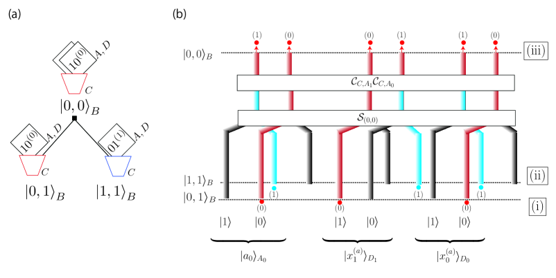
Figure 6: (a): An example of the output scheme $\mathcal{F}^{\dagger}$ (4.4) at a node $|0,0\rangle_{B}$ for $n=1$ and $m=2$. (b): A representation of (a) by quantum walkers (see also (4.1)–(4.3) as examples of the representation of states). (i), (ii) and (iii) represents the states (i) $|0,1\rangle_{B}|0\rangle_{C}|0\rangle_{A}|10^{(0)}\rangle_{D}$, (ii) $|1,1\rangle_{B}|1\rangle_{C}|1\rangle_{A}|01^{(1)}\rangle_{D}$ and (iii) $|0,0\rangle_{B}|0\rangle_{C}\left(|0\rangle_{A}|10^{(0)}\rangle_{D}+|1\rangle_{A}|01^{(1)}\rangle_{D}\right)$, respectively. Note that the actual implementation of the operators $\mathcal{S}$ (2.3) and $\mathcal{C}$ (3.10) by some scattering processes of multiple quantum walkers on properly constructed rails is left as a future task.

Our proposal for qRAM might be useful to design a qRAM architecture with simpler structures due to the following reasons. First, the routing and output scheme might be represented as some multi-particle scattering processes on suitably constructed graphs at each node, and therefore our bucket brigade qRAM does not need any quantum devices (e.g. qudits) at the nodes, but only needs $m+n$ quantum particles as quantum resources. Second, the quantum walkers are not entangled with the nodes. Thus, the three schemes, i.e. the routing, querying and output schemes can be achieved completely independently, and hence a full parallelization can be easily accomplished. This is in contrast to the original bucket brigade scheme [9, 10], where we must maintain the coherence between the bucket and the $O(n)$ nodes on the route: some ingenuity needs for a fully parallelization (see [16] for instance). Finally, since the three schemes can be described as dynamics of the quantum walkers, we could design qRAM with no need of time-dependent control.

5 Concluding remarks

In summary, we have provided a new concept of bucket brigade qRAM utilizing a quantum walk. Controlling a quantum motion of the quantum bucket with chirality, we can efficiently deliver the bucket to the desired memory cell, and fill the bucket with data stored in cells. Since our qRAM does not rely on quantum switches for the routing scheme, the bucket is free from the entanglement with the nodes. Alternatively, it uses the chirality state, which entangles with the address bits for a short amount of time, to navigate the quantum walker. Our qRAM may be more robust against quantum decoherence compared to the conventional bucket brigade method where it is required to maintain quantum coherence in all the activated qutrits.

The actual implementation of our algorithms by scattering processes of quantum walkers on properly constructed graphs [20, 21, 22] remains a future problem. It may also be of interest to apply our qRAM to quantum information processing, for instance image processing and transformations utilizing quantum version of fast Fourier transform [23], where the generation of multiple quantum images is crucial.

References

• [1] Grover L K 1996 A fast quantum mechanical algorithm for database search Proc. ACM STOC 212-219
• [2] Harrow A W, Hassidim A and Lloyd S (2009) Quantum algorithm for linear systems of equations Phys. Rev. Lett. 103 150502
• [3] Lloyd, S, Mohseni M, Rebentrost P 2014 Quantum principal component analysis Nature Physics 10 631
• [4] Lloyd S, Mohseni M, Rebentrost P 2013 Quantum algorithms for supervised and unsupervised machine learning arXiv:1307.0411
• [5] Rebentrost P, Mohseni M and Lloyd S 2014 Quantum support vector machine for big data classification Phys. Rev. Lett. 113 130503
• [6] Biamonte J, Wittek P, Pancotti N, Rebentrost P, Wiebe N and Seth Lloyd S 2017 Quantum machine learning Nature 549 195-202
• [7] Schuld M, Fingerhuth M, Petruccione F 2017 Implementing a distance-based classifier with a quantum interference circuit Europhys. Lett. 119 60002
• [8] Bang J, Dutta A, Lee S W, and Kim J 2019 Optimal usage of quantum random access memory in quantum machine learning Phys. Rev A 99 012326
• [9] Giovannetti V, Lloyd S and Maccone L 2008 Quantum Random Access Memory Phys. Rev. Lett. 100 160501
• [10] Giovannetti V, Lloyd S and Maccone L 2008 Architectures for a quantum random access memory Phys. Rev. A 78 052310
• [11] Jaeger R C and Blalock T N 2003 Microelectronic Circuit Design (Dubuque, IA: McGraw-Hill)
• [12] Sedra A S and Smith K C 1998 Microelectronic Circuits (New York: Oxford University Press)
• [13] Hong F-Y, Xiang Y, Zhu Z-Y, Jiang L-z and Wu L-n 2012 Robust quantum random access memory Phys. Rev. A 86 010306
• [14] Arunachalam S, Gheorghiu V, Jochym-Oโ€™Connor T, Mosca M and P. V. Srinivasan P V 2015 On the robustness of bucket brigade quantum RAM New J. Phys. 17 123010
• [15] Matteo O D, Gheorghiu V and Mosca M 2020 Fault-Tolerant Resource Estimation of Quantum Random-Access Memories IEEE Transactions on Quantum Engineering 1 4500213
• [16] Paler A, Oumarou O and Basmadjian R 2020 Parallelizing the queries in a bucket-brigade quantum random access memory Phys. Rev. A 102 032608
• [17] Park D K, Petruccione F and Rhee J-K K 2019 Circuit-Based Quantum Random Access Memory for Classical Data Sci. Rep. 9:3949
• [18] Aharonov Y, Davidovich L, Zagury N 1993 Quantum random walks Phys. Rev A 48 1687
• [19] Venegas-Andraca, S E 2012 Quantum walks: a comprehensive review Quantum Inf. Process. 11 1015
• [20] Andrew M. Childs A M, Gosset D and Webb Z 2013 Universal Computation by Multiparticle Quantum Walk Science 339 791
• [21] Childs A M 2009 Universal Computation by Quantum Walk Phys. Rev. Lett. 102 180501
• [22] Lovett N B, Cooper S, Everitt M, Trevers M and Kendon V 2010 Universal quantum computation using the discrete-time quantum walk Phys. Rev. A 81 042330
• [23] Asaka R, Sakai K, and Yahagi R 2020 Quantum circuit for the fast Fourier transform Quantum Inf. Process. 19 277