Robots, computer algebra and
eight connected components

Abstract

Answering connectivity queries in semi-algebraic sets is a long-standing and challenging computational issue with applications in robotics, in particular for the analysis of kinematic singularities. One task there is to compute the number of connected components of the complementary of the singularities of the kinematic map. Another task is to design a continuous path joining two given points lying in the same connected component of such a set. In this paper, we push forward the current capabilities of computer algebra to obtain computer-aided proofs of the analysis of the kinematic singularities of various robots used in industry.

We first show how to combine mathematical reasoning with easy symbolic computations to study the kinematic singularities of an infinite family (depending on paramaters) modelled by the UR-series produced by the company “Universal Robots”. Next, we compute roadmaps (which are curves used to answer connectivity queries) for this family of robots. We design an algorithm for “solving” positive dimensional polynomial system depending on parameters. The meaning of solving here means partitioning the parameter’s space into semi-algebraic components over which the number of connected components of the semi-algebraic set defined by the input system is invariant. Practical experiments confirm our computer-aided proof and show that such an algorithm can already be used to analyze the kinematic singularities of the UR-series family. The number of connected components of the complementary of the kinematic singularities of generic robots in this family is $8$.

1 Introduction

The individual parts of a serial robot, called links, are moved by controlling the angle of each joint connecting two links. The inverse kinematics problem asks for the values of all angles producing a desired position of the end effector, where “position” includes not just the location of the end effector in 3-space but also the orientation. In a sense, this means inverting a function which is called the forward kinematics map in robotics, which determines the position of the end effector for given angles by a well-known formula (see Section 2). In robot controlling, the inverse kinematics problem is often solved incrementally: starting from some known initial angle configuration and its corresponding end effector position, we want to compute the change of the angles required to achieve a desired small change in the end effector position.

Kinematic singularities are defined as critical points of the forward map, i.e. angle configurations where the Jacobian matrix of the forward map is rank deficient. There are two known facts that make rather difficulty to control a robot in a singular or near a singular configuration. First, if an end effector velocity or force outside the image of the singular Jacobian is desired, then the necessary joint velocity or torque is either not defined or very large (see [23] §4.3 and [31] §5.9). The second reason is that industrial controllers are based on Newton’s method for the incremental solution of the inverse problem, and this method is not guaranteed to converge if it is used with a starting point close to the singular set. For these reasons, engineers prefer to plan the robot movements avoiding kinematic singularities.

For a general serial robot with six joints, the singular set is a hypersurface defined locally by the Jacobian determinant of the forward map. Its complementary, a real manifold, is not connected. Counting the number of connected components of this manifold and answering connectivity queries in this set is then of crucial importance in this application domain.

Answering connectivity queries in semi-algebraic sets is a classical problem of algorithmic semi-algebraic geometry which has attracted a lot of attention through the development of the so-called ROADMAP algorithms (see e.g. [12, 11, 9, 6, 8, 27, 28, 21]). Up to our knowledge, such algorithms had never been developed enough and implemented efficiently to tackle real-life applications.

In this paper, we push forward the capabilities of computer algebra in this application domain by solving connectivity queries for the non singular configuration sets of industrial robots from the UR series of the company “Universal Robots”. For a particular robot in this series, the UR5, the number of components of the non singular configuration set is 8 (see Section 3). For two points in the same component, we show how to construct a connecting path, in two ways: either by an ad hoc way (which has its own algorithmic interest) taking advantage of the specialty of the geometric parameters of UR5, and by using the ROADMAP algorithm (see Section 5). Next, we go further and extend our analysis of UR5 to the whole UR series and prove that outside a proper Zariski closed set (UR5 is outside this closed set) the number of connected components of the non singular configuration set is constant. These are computer-aided mathematical proofs involving <<easy>> symbolic computations

The next contribution is based on the fact that the family of UR robots is determined by a finite list of real parameters. Hence, an algorithmic way of tackling the problem of analyzing kinematic singularities of the whole UR family is to <<solve>> a positive dimensional system depending on parameters (i.e. after specialization of the parameters, the specialized system is positive dimensional). We design an algorithm that decomposes the parameter’s space into semi-algebraic subsets, such that the number of connected components of the non singular configurations is constant in each of these subsets. As far as we know, this is the first algorithm of that type which is designed.

We also implemented this algorithm and used it for the analysis of the kinematic singularities of the UR series. Computations are heavy but already doable (on a standard laptop) within $10$ hours. This is a computational way to retrieve the same results as our computer-aided mathematical proofs. These computations show that computer algebra today is efficient enough to solve connectivity queries that are of practical interest in industrial robot applications.

2 Robotics problem formulation

We define a manipulator or robot as follows: we have finite ordered rigid bodies called links which are connected by $n$ revolute joints that are also ordered. To each joint we associate a coordinate system or a frame. The links are connected in a serial manner i.e. if we consider the robot as a graph such that the vertices are joints and the edges are links then this graph is a path (the first and last joint has degree 1 and all other joints have degree 2) and the joints allow rotation about its axes, so that if a joint rotates then all other subsequent links rotate about the axes of this joint. A reference coordinate system is chosen for the final joint which is called the end-effector.

In theoretical kinematics one may forget that the links are rigid bodies so that collision between links are disregarded. In this case we may as well think of a robot as a differentiable map $F:\mathrm{SO}(2)^{n}\longrightarrow\mathrm{SE}(3)$ where $\mathrm{SO}(2)$ is the one-dimensional group of rotations around a fixed line, parameterised by the rotation angle, and $\mathrm{SE}(3)$ is the six-dimensional group of Euclidean congruence transformations. This map is defined in the following way:

• The $i$-th coordinate of an element in $\mathrm{SO}(2)^{n}$ is associated to the $i$-th (revolute) joint parameter.

• For joint values $\vec{\theta}:=(\theta_{1},\dots,\theta_{n})$ in $\mathrm{SO}(2)^{n}$, the image $F(\vec{\theta})$ is the transformation of the end-effector from the initial position corresponding to all angles being zero to the final position obtained by composing the $n$ rotations.

The map $F$ itself is called the kinematic map (of the robot). Its domain is called the configuration space, while its image is called the work-space or the kinematic image.

We use the Denavit-Hartenberg (DH) convention when describing relations between two joint frames. It is standard in robotics ; its advantages are discussed in e.g. [31, §3.2], [1, §4.2]. The transformation between the frames is given by the following rule:

• The $z$-axis of the reference frame will be the axis of rotation of the joint.

• To obtain the next frame, one starts with a rotation about the $z$-axis of the reference frame, called the rotation, followed by

• a translation along the $z$-axis of the reference frame, called the offset, followed by

• a translation along the $x$-axis, called the distance, followed by

• a rotation about the $x$-axis, called the twist.

The transformation between frame $i$ to frame $i+1$ is

$$R_{z}(\theta_{i})T_{z}(d_{i})T_{x}(a_{i})R_{x}(\alpha_{i})$$

where $R_{z},T_{z},T_{x},R_{x}$ are rotations or translations with respect to $z$- or $x$-axis parameterised by the angle of rotation $\theta_{i}$ (the $i$-th joint parameter), the offset $d_{i}$, the distance $a_{i}$ and the angle of twist $\alpha_{i}$ of the $i$-th frame. For a given robot with $n$ joints all DH parameters except for the rotation are fixed values. So that image of $F$ for given joint values (the rotations) $(\theta_{1},\dots,\theta_{n})$ is just the multiplication of these transformations in $\mathrm{SE}(3)$. The parameters $d_{1},d_{n},a_{n},\alpha_{n}$ are assumed to be $0$. This is not a loss of generality, because we can freely choose the frame at the base and at the end-effector. More detailed discussion on these can be seen in [31].

Example 2.1.

The UR5 robot has the following DH parameters:
distances (m.) $(a_{1},\dots,a_{6}):=(0,-\frac{425}{1000},-\frac{39225}{100000},0,0,0)$
offsets (m.) $(d_{1},\dots,d_{6}):=(0,0,0,\frac{10915}{100000},\frac{9465}{100000},0)$
twist angles (rad.) $(\alpha_{1},\dots,\alpha_{6}):=(\frac{\pi}{2},0,0,\frac{\pi}{2},-\frac{\pi}{2},0)$

For example, the following joint angles (rotations, in rad.)

$$(\theta_{1},\dots,\theta_{6}):=\left(\frac{1}{10},\frac{2}{10},\frac{3}{10},\frac{4}{10},\frac{5}{10},\frac{6}{10}\right)$$

leads to the following transformation in $(R,\vec{t})\in\mathrm{SE}(3)$ (represented as elements in $\mathrm{SO}(3)\rtimes\mathbb{R}^{3}$) where:

$$R\simeq\begin{pmatrix}0.047&-0.977&-0.209\\ -0.393&0.174&-0.903\\ 0.918&0.123&-0.376\end{pmatrix},\ \vec{t}\simeq(-6.768,-1.7784,-3.336).$$

Definition.

Given the kinematic map of a manipulator $F:\mathrm{SO}(2)^{n}\rightarrow\mathrm{SE}(3)$, the kinematic singularities in the configuration space are the points $P\in(\mathbb{P}^{1})^{n}$ such that the Jacobian of $F$ at $P$ is rank-deficient.

In this paper, we will only deal with 6-jointed manipulators. Therefore the kinematic map is a differentiable map from the 6-dimensional configuration space $(\mathrm{SO}(2))^{6}$ to the group $\mathrm{SE}(3)$, which is also $6$-dimensional. For non-singular points of the map, the Jacobian is therefore invertible, and $F$ is a local homeomorphism. Here is a well-known geometric description of singularities.

Theorem 2.2.

Let $F:\mathrm{SO}(2)^{6}\rightarrow\mathrm{SE}(3)$ be the kinematic map of a robot with 6 joints. Let $P\in\mathrm{SO}(2)^{6}$. Then the following are equivalent.

1. $P$ is a kinematic singularity.

2. The Jacobian of $F$ at $P$ is singular.

3. If $P_{1},\dots,P_{6}\in\mathbb{P}^{5}(\mathbb{R})$ are the Plücker representation of the axes (lines in $\mathbb{P}^{3}$) of the joints of the robot at the configuration point $P$ then the matrix consisting of the Plücker coordinates $(p_{i,j})_{i,j\leq 6}$ ($P_{i}=(p_{i,1}:p_{i,2}:\cdots:p_{i,6})$ for $i=1,\dots,6$) is singular.

Proof.

The equivalence of the first two items is clear by definition. The equivalence of the first and the third item is found in [30, §4.5.1], [23, §4.1] or [1, §4.5.1.] ∎

Assume that we have two non-singular points in the configuration set. As explained earlier, we want to decide if these two configurations can be connected by a curve of configurations which avoids the singular hypersurface (see [33] §1.2 for some history on this question). If yes, then an explicit construction of such a curve is also of interest. In order to tackle these problems, we choose parameters for $\mathrm{SO}(2)$ so that the equation of the hypersurface becomes a polynomial. This is not the case when we use the angles $\theta_{1},\dots,\theta_{n}$, because the Jacobian contains trigonometric functions in these angles. One well-known strategy is to parametrize by points on a unit circle, i.e. by two parameters satisfying the equation of the unit circle. This has a clear disadvantage: the number of variables increases, and the singular set has co-dimension greater than one. Another well-known strategy is to replace $\theta_{i}$ by $v_{i}=\tan\frac{\theta_{i}}{2}$. The variable $v_{i}$ ranges over the projective line, and the angle $\pi$ corresponds to the point at infinity. If we set $v_{i}=\tan\frac{\theta_{i}}{2}$ for $i=1,\dots,n$, then we obtain, in general, a polynomial in $v_{2},\dots,v_{5}$. More precisely, the degree is 2 in $v_{2}$ and $v_{5}$ and degree 4 in $v_{3}$ and in $v_{4}$. The Jacobian does not depend on the joint angles $\theta_{1}$ and $\theta_{6}$. This is clear from the third characterization of singularities in Theorem 2.2: only the position of the axes are relevant, and a rotation along the first or the last axis does not change the position of any axis.

We define the UR Family to be robots having a similar DH-parameter as the known UR robots (UR5, UR10, etc.). Such UR robots are parameterised by the following DH parameters
distances (m.) $(a_{1},\dots,a_{6}):=(0,a_{2},a_{3},0,0,0)$
offsets (m.) $(d_{1},\dots,d_{6}):=(0,0,0,d_{4},d_{5},0)$
twist angles (rad.) $(\alpha_{1},\dots,\alpha_{6}):=(\frac{\pi}{2},0,0,\frac{\pi}{2},-\frac{\pi}{2},0)$

For these robots, the determinant of the Jacobian (see [34]), expressed as a polynomial in $v_{2},\dots,v_{5}$, is $A=-Bv_{3}v_{5}$ with

$$B=a_{2}v_{2}^{2}v_{3}^{2}v_{4}^{2}-a_{3}v_{2}^{2}v_{3}^{2}v_{4}^{2}-2d_{5}v_{2}^{2}v_{3}^{2}v_{4}-2d_{5}v_{2}^{2}v_{3}v_{4}^{2}-2d_{5}v_{2}v_{3}^{2}v_{4}^{2}+a_{2}v_{2}^{2}v_{3}^{2}+a_{2}v_{2}^{2}v_{4}^{2}-a_{2}v_{3}^{2}v_{4}^{2}-a_{3}v_{2}^{2}v_{3}^{2}+a_{3}v_{2}^{2}v_{4}^{2}+4a_{3}v_{2}v_{3}v_{4}^{2}+a_{3}v_{3}^{2}v_{4}^{2}+2d_{5}v_{2}^{2}v_{3}+2d_{5}v_{2}^{2}v_{4}+2d_{5}v_{2}v_{3}^{2}+8d_{5}v_{2}v_{3}v_{4}+2d_{5}v_{2}v_{4}^{2}+2d_{5}v_{3}^{2}v_{4}+2d_{5}v_{3}v_{4}^{2}+a_{2}v_{2}^{2}-a_{2}v_{3}^{2}-a_{2}v_{4}^{2}+a_{3}v_{2}^{2}+4a_{3}v_{2}v_{3}+a_{3}v_{3}^{2}-a_{3}v_{4}^{2}-2d_{5}v_{2}-2d_{5}v_{3}-2d_{5}v_{4}-a_{2}-a_{3}$$

Note that there is a degree drop in three of the four cases: the degree in $v_{3}$ is only $3$, and not $4$, and the degree in $v_{4}$ is only $2$, and not $4$, and the degree in $v_{5}$ is only $1$, and not $2$. The drop in the degree means that the homogeneous form of the Jacobian has a linear factor that vanishes if and only if the value of the variable whose degree drops is infinity, or equivalently, that the corresponding angle is $\pi$. Since we are interested in the complement of the singular space, we may assume that none of these three angles is equal to $\pi$, and we can use the parameters $v_{3},v_{4},v_{5}$ without worrying about paths crossing infinity.

For the angle $\theta_{2}$, the situation is different. There is no degree drop, hence there are configurations with $\theta_{2}=\pi$ in the non singular configuration set. If we use the parametrization by half angle, then we have to take paths in the projective line into account that cross infinity, or, in other words, consider this variable in the projective space $\mathbb{P}^{1}(\mathbb{R})$. But, to take advantage on algorithms acting on semi-algebraic sets, one needs variables that range over $\mathbb{R}$.

Hence, we instead use parameters $s_{2}=\sin(\theta_{2})$ and $c_{2}=\cos(\theta_{2})$ and add the additional equation $s_{2}^{2}+c_{2}^{2}=1$, obtaining a polynomial in the variables $s_{2},c_{2},v_{3},v_{4},v_{5}$ with coefficients depending on the parameters $a_{2},a_{3},d_{4},d_{5}$. Of course, the reason for this more costly treatment for $\theta_{2}$ is just necessary if we use the ROADMAP algorithm subsequently. For an alternative analysis not using it, it is still better to use the half tangent ranging over the projective line.

3 Analysis of the UR5 Robot

We gave in Example 2.1 the Denavit-Hartenberg parameters of the UR5 robot. These values are used to instantiate $a_{2},a_{3}$ and $d_{5}$ in the above polynomial $B$; the specialized polynomial is then denoted by $\tilde{B}$ and we let $\tilde{A}=\tilde{B}v_{3}v_{5}$. Recall that $v_{2}$ ranges over $\mathbb{P}^{1}$, while $v_{3},v_{4},v_{5}$ range only over the affine line.

We investigate the discriminant of $\tilde{B}$ with respect to the variable $v_{2}$ (thus the projection of the critical set to the $(v_{3},v_{4})$-plane). The discriminant of $\tilde{B}$ with respect to the variable $v_{2}$ we denote as $b\in\mathbb{R}[v_{3},v_{4}]$. This discriminant is still factorisable in $\mathbb{C}[v_{3},v_{4}]$. In fact, one checks, that it is the factor of two complex conjugates of some polynomial in $\mathbb{R}[v_{3},v_{4}]$. This implies that $b=c^{2}+d^{2}$ is the sum of two squares of real polynomials $c,d\in\mathbb{R}[v_{3},v_{4}]$. These two polynomials are given by

$$c =\frac{1577212v_{3}-3561263v_{4}-14850585}{\sqrt{2006237}}$$

$$d =\frac{(\sqrt{2006237}v_{4}+1239915-7144712)v_{3}+16090500v_{4}}{\sqrt{2006237}}$$

Thus, $b$ can have only two real roots (i.e. two pairs $(v_{3},v_{4})$), i.e the vanishing set of $b$ in $\mathbb{R}^{2}$ is finite, namely they points that are the zeros of both $c$ and $d$. We solve this as floating numbers to have an idea of their vicinity in an affine chart of the ambient space of the kinematic singularity. The roots are

$$\begin{array}[]{llll}q_{1}&=(v_{3}\simeq-9.140975564&,&v_{4}\simeq-8.218388067)\\ q_{2}&=(v_{3}\simeq 9.140975563&,&v_{4}\simeq-.1216783622)\end{array}$$

For the two special values $q_{1}$ and $q_{2}$ in the $(v3,v4)$-plane, all three coefficients of $\tilde{B}$ with respect to $v_{2}$ are zero.

Now, since the discriminant $b$ is positive except at these two points and since $\tilde{B}$ itself is quadratic with respect to $v_{2}$ we conclude that the preimage of the projection (to $(v_{3},v_{4})$-plane) are two real points in the variety defined by $\tilde{B}$. Thus, the variety defined by $\tilde{B}$ is composed of two sheets (above any two points $(v_{3},v_{4})$ except $q_{1}$ and $q_{2}$). Let $X$ be the complement of the vanishing points of $\tilde{B}$ in $\mathbb{P}^{1}\times\mathbb{A}^{2}$. Set

$$Y:=\mathbb{A}^{2}\setminus(\{q_{1},q_{2}\}\cup\{(0,v_{4})\mid v_{4}\in\mathbb{R}\})$$

So we have a canonical projection (to the $(v_{3},v_{4})$-plane) from $X\cap(\mathbb{P}^{1}\times Y)$ to $Y$. The fiber of this projection is a projective line without two distinct points. Hence, every fiber has two components. The sign of $\tilde{B}$ is different for the two components of each fiber. Then, we have two components of $X$ for each component of $Y$. Obviously, $Y$ has two components, hence we have a total number of $4$ components.

For the non singular set, which is the complement of the zero set of $\tilde{A}$, we get $8$ components: for each component of $X$, we have one component where $v_{5}$ is positive and one where $v_{5}$ is negative.

Now assume that we have two non singular configuration points $x,y$ in the same component, and we want to construct a path connecting them. The projections to $Y$ have to lie in the same component of $Y$, and because $Y$ is the plane without a line and two points, it is easy to connect the images of the projections in $Y$: in most cases, a straight line segment is fine; if the straight line segment connecting the two image points contains $q_{1}$ or $q_{2}$, we have to do a random detour via a third point. The zero set of $\tilde{B}$ is a two-sheeted covering of $Y$. So, for any value of $Y$, we have two points in the zero set of $\tilde{B}$ projecting to it. If we look at these points as points in $\mathrm{SO}(2)$, then it is clear that there are two “midpoints” in the zero set of $\tilde{B}$, which have equal angle distance to these two points. The value of $\tilde{B}$ is positive for one of the two midpoints and negative for the other one. The sign of $\tilde{B}(x)$ and $\tilde{B}(y)$, however, must be the same because the two points are in the same connected component. Suppose, without loss of generality, that $\tilde{B}(x)$ and $\tilde{B}(y)$ are both positive. Then we first connect $x$ to the midpoint over the projection of $x$ to $Y$ with positive sign, by a curve in the fiber. Next, we lift the path in $Y$, connecting the projections of $x$ and $y$ in the same component, to a path of midpoints with positive sign, arriving at the midpoint with positive sign lying over the projection of $y$. Finally, we connect this midpoint to $y$ by the other fiber.

Below, we show the sheets in Figure 1 to illustrate that:

1. the regions above and below the sheets can be connected

2. the region between the two sheets is the other connected component

3. the two points $q_{2}$ and $q_{3}$ are points in the projection where the sheets get connected (see assymptotes in Fig. 1). Thus, the variety describing the two sheets is connected.

Figure 1: The two sheets of $\tilde{B}$

4 UR series

We can make a general statement for robots belonging to the UR family (e.g. UR10, UR3 etc. ). We define the UR Family to be robots which have a similar DH-parameter as the known UR robots (UR5, UR10 etc.), a robot in this family we shall call a UR robot. Namely they are parameterised by the following DH parameters :
distances (m.) $(a_{1},\dots,a_{6}):=(0,a_{2},a_{3},0,0,0)$
offsets (m.) $(d_{1},\dots,d_{6}):=(0,0,0,d_{4},d_{5},0)$
twist angles (rad.) $(\alpha_{1},\dots,\alpha_{6}):=(\frac{\pi}{2},0,0,\frac{\pi}{2},-\frac{\pi}{2},0)$

i.e. these robots are parameterised by $4$ parameters: $a_{2},a_{3},d_{4},d_{5}$.

We can write the largest (in number of terms and in degree) polynomial factor of the polynomial whose vanishing points is the kinematic singularity in configuration space of a UR robot as

$$B=a_{2}v_{2}^{2}v_{3}^{2}v_{4}^{2}-a_{3}v_{2}^{2}v_{3}^{2}v_{4}^{2}-2d_{5}v_{2}^{2}v_{3}^{2}v_{4}-2d_{5}v_{2}^{2}v_{3}v_{4}^{2}-2d_{5}v_{2}v_{3}^{2}v_{4}^{2}+a_{2}v_{2}^{2}v_{3}^{2}+a_{2}v_{2}^{2}v_{4}^{2}-a_{2}v_{3}^{2}v_{4}^{2}-a_{3}v_{2}^{2}v_{3}^{2}+a_{3}v_{2}^{2}v_{4}^{2}+4a_{3}v_{2}v_{3}v_{4}^{2}+a_{3}v_{3}^{2}v_{4}^{2}+2d_{5}v_{2}^{2}v_{3}+2d_{5}v_{2}^{2}v_{4}+2d_{5}v_{2}v_{3}^{2}+8d_{5}v_{2}v_{3}v_{4}+2d_{5}v_{2}v_{4}^{2}+2d_{5}v_{3}^{2}v_{4}+2d_{5}v_{3}v_{4}^{2}+a_{2}v_{2}^{2}-a_{2}v_{3}^{2}-a_{2}v_{4}^{2}+a_{3}v_{2}^{2}+4a_{3}v_{2}v_{3}+a_{3}v_{3}^{2}-a_{3}v_{4}^{2}-2d_{5}v_{2}-2d_{5}v_{3}-2d_{5}v_{4}-a_{2}-a_{3}$$

Note that $d_{4}$ does not affect the singularity of the robot. Taking the discriminant of $B$ with respect to $v_{2}$ yields the sum of two squares i.e. the product of two quadratic complex conjugate polynomials $\operatorname{disc}(B,v_{2})=g\overline{g}$.

$$g=(-a_{2}v_{3}v_{4}+a_{3}v_{3}v_{4}+d_{5}v_{3}+d_{5}v_{4}+a_{2}+a_{3})+(-d_{5}v_{3}v_{4}+a_{2}v_{3}+a_{2}v_{4}-a_{3}v_{3}+a_{3}v_{4}+d_{5})i$$

For a robot determined by some real quadruple $u\in\mathbb{R}^{4}$, let $A_{u},B_{u},g_{u}$ be the polynomials obtained by instantiating in $A,B,g$ the variables $a_{2},a_{3},d_{4},d_{5}$ by the corresponding real values in the quadruple. Let $f:\mathbb{R}^{3}\to\mathbb{R}^{2}$ be the projection $(v_{2},v_{3},v_{5})\mapsto(v_{3},v_{5})$. Let $Y_{u}\subset\mathbb{R}^{2}$ be the complement of (the union of the line $v_{3}=0$ and the common zero set of $\operatorname{Re}g_{u}$ and $\operatorname{Im}g_{u})$. Then the real zero set of $B_{u}$ in $\mathbb{R}^{3}$ intersected with $f^{-1}(Y_{u})$ projects to surjectively to $Y_{u}$, in such a way that there are two sheets, each projecting homeomorphically to $Y_{u}$.

For general robot $u$, the real set of $g$, which is meaning the set of all points in the real $(v_{3},v_{4})$-plane such that both the real part and the imaginary part of $g$ is equal to zero, is a finite subset of $\mathbb{R}^{2}$. All arguments from the previous sections work in this case as well. Hence we get $8$ components for these parameters’values. Moreover, we have paths connecting points in the same component, as in the previous section.

It remains to treat the non-general robots where the real zero set of $g$ is one-dimensional. This is the case if and only if $d_{5}=a_{2}^{2}-a_{3}^{2}=0$. The even more special case $d_{5}=a_{2}=a_{3}=0$ is easy to analyze: here, the determinant of the Jacobian $A$ is identically zero, which means that there are no non singular configurations. Excluding that case, we have two families of robots, and in each family, up to the value of $d_{4}$, the parameters are unique up to scaling. Without loss of generality, we can reduce to exactly two non-general robots $u^{\prime}=(1,1,0,0)$ and $u^{\prime\prime}=(1,-1,0,0)$. Then the polynomial $B_{u^{\prime}}$ has a factor is $C^{\prime}:=v_{3}v_{4}-v_{3}-v_{4}-1$, and the polynomial $B_{u^{\prime\prime}}$ has a factor $C^{\prime\prime}:=v_{3}v_{4}+v_{3}+v_{4}-1$. Apart from that complication, the analysis proceeds similar as in the general case: the set $Y_{u^{\prime}}$ is the plane minus the line $v_{3}=0$ minus the hyperbola with equation $C^{\prime}$, and the set $Y_{u^{\prime\prime}}$ is the plane minus the hyperbola with equation $C^{\prime\prime}$. In both cases, the number of components of $Y$ is 5, as it can be seen in Figure 2. Consequently, we have 20 components in total. The paths between points in the same component can be constructed similarly as in the general case.

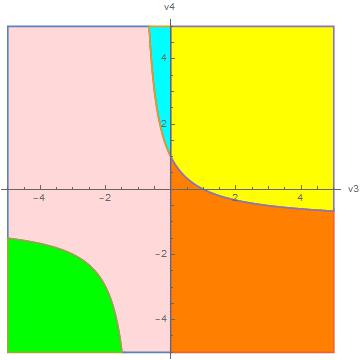
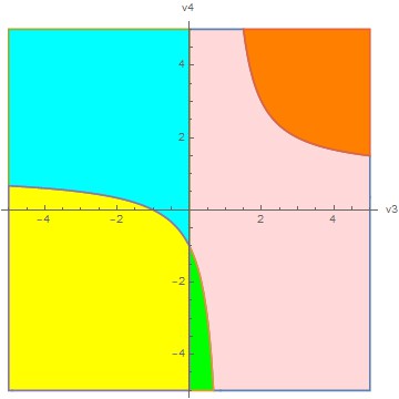
Figure 2: Left (resp. right) shows the components of $v_{3}(v_{3}v_{4}+v_{3}+v_{4}-1)\neq 0$ (resp. $v_{3}(v_{3}v_{4}-v_{3}-v_{4}-1)\neq 0$) in $Y$

5 Connectivity and roadmaps

We explain the ROADMAP algorithm for the special case where the semi-algebraic set $S$ is given as a subset of some vector space $\mathbb{R}^{N}$, $N\in\mathbb{N}$, defined by an equation $f(x_{1},\dots,x_{N})=0$ and an inequation $g(x_{1},\dots,x_{N})\neq 0$. We assume that the algebraic set defined by $f=0$ is smooth. This is sufficient for our application: the inequation is the determinant of the Jacobian of the kinematic map $A$, and the equality is $s_{2}^{2}+c_{2}^{2}-1=0$.

One first reduces the problem to one where the semi-algebraic set we consider is bounded. Note that there exists $R>0$ large enough such that the connected components of $S$ are in one-to-one correspondence with the intersection of $S$ with the hyper-ball defined by $\mathscr{N}_{R}\leq 0$ where $\mathscr{N}_{R}=x_{1}^{2}+\cdots+x_{n}^{2}-R$. We denote this intersection by $S^{\prime}$. Note that a roadmap of $S^{\prime}$ provides a roadmap of $S$.

Determining such a large enough real number $R$ is done by choosing it larger than the largest critical value of the restriction of the map $\bm{x}\to\|\bm{x}\|^{2}$ to each regular strata of the the Euclidean closure of $S$. This leads us to compute critical values of that map restricted to the hypersurface defined by $f=0$ and next take the limits of the critical values of the sets defined by $g=\pm\varepsilon$ and $f=g\pm\varepsilon=0$ when $\varepsilon\to 0$.

Next, we compute the critical values $\eta_{1}<\cdots<\eta_{s}$ of the restriction of the map $\bm{x}\to g(\bm{x})$ to the semi-algebraic set defined by $f=0$ and $\mathscr{N}_{R}\leq 0$. Following Thom’s isotopy lemma [13], when $e$ is chosen between $0$ and $\min(|\eta_{i}|,1\leq i\leq s)$, the connected components of the semi-algebraic set $S^{+}_{e}$ (resp. $S^{-}_{e}$) defined by $\mathscr{N}_{R}\leq 0,f=g-e=0$ (resp. $\mathscr{N}_{R}\leq 0,f=g+e=0$) are in one-to-one correspondence with the connected components of the semi-algebraic set defined by $\mathscr{N}_{R}\leq 0,f=0,g>0$ (resp. $\mathscr{N}_{R}\leq 0,f=0,g>0$). Besides, $S^{+}_{e}\subset S^{\prime}$ (resp. $S^{-}_{e}\subset S^{\prime}$). Then a roadmap of $S^{\prime}$ is obtained by taking the union of a roadmap of $S^{+}_{e}$ with the roadmap of $S_{e}^{-}$. Hence, we have performed a reduction to computing roadmaps in the compact semi-algebraic sets $S_{e}^{+}$ and $S_{e}^{-}$.

In our application, the algebraic sets defined by the vanishing of all subsets of the defining polynomials of $S_{e}^{+}$ and $S_{e}^{-}$ are smooth. Hence, we can rely on a slight modification of the roadmap algorithm given in [12] where we replace computations with multivariate resultants for solving polynomial systems by computations of Gröbner bases.

The algorithm in [12] then takes as input a polynomial system defining a closed and bounded semi-algebraic set $S$ and proceeds as follows. The core idea is to start by computing a curve $\mathscr{C}$ which has a non-empty intersection with each connected component of $S$. That curve will be typically the critical locus on the $(x_{1},x_{2})$-plane when one is in generic coordinates (else, one just needs to change linearly generically the coordinate system). A few remarks are in order here. When $S$ is defined by $f_{1}=\cdots=f_{p}=0$ and $g_{1}\geq 0,\cdots,g_{s}\geq 0$, to define the critical locus of the projection on the $(x_{1},x_{2})$-plane restricted to $S$ one takes the union of the critical loci of that projection restricted to the real algebraic sets defined for all $\{i_{1},\ldots,i_{\ell}\}\subset\{1,\ldots,s\}$, by $f_{1}=\cdots=f_{p}=g_{i_{1}}=\cdots=g_{i_{\ell}}=0$ and intersect this union of critical loci with $S$ (see [12]).

That way, one obtains curves that intersect all connected components of $S$ but these intersections may not be connected. To repair these connectivity failures, Canny’s algorithm finds appropriate slices of $S$. Let $\pi_{1}$ be the canonical projection $(x_{1},\ldots,x_{n})\to x_{1}$. This basically consists in finding $\alpha_{1}<\ldots<\alpha_{k}$ in $\mathbb{R}$ such that the union of $\cup_{i=1}^{k}S\cap\pi_{1}^{-1}(\alpha_{i})$ with the critical curve $\mathscr{C}$ has a non-empty and connected intersection with each connected component of $S$.

The way Canny proposes to find those $\alpha_{i}$’s is to compute the critical values of the restriction of $\pi_{1}$ to $\mathscr{C}$. By the algebraic Sard’s theorem (see e.g. [28, Appendix B]), these values are in finite number and Canny proposes to take $\alpha_{1},\cdots,\alpha_{k}$ as those critical values. This leads to compute with real algebraic numbers which can be encoded with their minimal polynomials and isolating intervals. Since these minimal polynomials may have large degrees (singly exponential in $n$), that step can be prohibitive for practical computations. We use then the technique introduced in [22] which consists in replacing $\alpha_{1}<\cdots<\alpha_{k}$ with rational numbers $\rho_{1}<\cdots<\rho_{k-1}$ with $\alpha_{i}<\rho_{i}<\alpha_{i+1}$. We refer to [22] for the rationale justifying this trick. All in all, one obtains a recursive algorithm with a decreasing number of variables at each recursive call. Combined with efficient Gröbner bases engines, we illustrate in Section 7 that the ROADMAP algorithm (with the modifications introduced above) can be used in practice to answer connectivity queries in semi-algebraic sets in concrete applications.

The concept of roadmap and the algorithm computing it, described above, may seem cumbersome and unnecessarily sophisticated, especially when compared with the much more direct CAD approach [29]. The CAD algorithm is also a recursive algorithm, producing its recursive instance by projecting the hypersurface to $\mathbb{R}^{n+1}$ and analyzing the discriminant. This leads to an iteration of discriminants, and it is easy to see that the degree of the iterated discriminants grows double exponentially in $n$: roughly, the degree of the discriminant is squared in every iteration. There lies the motivation for all the sophistication of the ROADMAP algorithm: for each instance in the all recursive calls, the degree of the input polynomial is exactly the same as the degree of the initially given polynomial $f$. This leads to an asymptotic complexity which is only single exponential in $n^{2}$. We refer to [27, 9, 28, 8] for more recent algorithms improving the complexity of roadmap computations.

6 Parametric polynomial systems

Let $F=(f_{1},\ldots,f_{p})$ and $G=(g_{1},\ldots,g_{q})$ in $\mathbb{Q}[\bm{x},\bm{y}]$ with $\bm{x}=(x_{1},\ldots,x_{n})$ and $\bm{y}=(y_{1},\ldots,y_{t})$. We consider further $\bm{y}$ as a sequence of parameters and the polynomial system

$$f_{1}=\cdots=f_{p}=0,\qquad g_{1}\ \sigma_{1}\ 0,\;\ldots,\;g_{q}\ \sigma_{q}\ 0$$

with $\sigma_{i}\in\{>,\geq\}$. We let $S\subset\mathbb{R}^{n}\times\mathbb{R}^{t}$ be the semi-algebraic set defined by this system. For $y\in\mathbb{R}^{t}$, we denote by $F_{y}$ and $G_{y}$ the sequences of polynomials obtained after instantiating $\bm{y}$ to $y$ in $F$ and $G$ respectively. Also, we denote by $S_{y}\subset\mathbb{R}^{n}$ the semi-algebraic set defined by the above system when $\bm{y}$ is specialized to $y$. The algebraic set defined by the simultaneous vanishing of the entries of $F$ (resp. $F_{y}$) is denoted by $V(F)\subset\mathbb{C}^{n+t}$ (resp. $V(F_{y})\subset\mathbb{C}^{n}$).

We describe an algorithm for solving such a parametric polynomial system without assuming that for a generic point $y$ in $\mathbb{C}^{t}$, $V(F_{y})$ is finite. In that situation, solving such a parametric polynomial system may consist in partitioning the parameters’space $\mathbb{R}^{t}$ into semi-algebraic sets $T_{1},\ldots,T_{r}$ such that, for $1\leq i\leq r$, the number of connected components of $S_{y}$ is invariant for any choice of $y$ in $T_{i}$. We prove below that such an algorithmic problem makes sense.

Proposition 6.1.

Let $S\subset\mathbb{R}^{n}\times\mathbb{R}^{t}$ be a semi-algebraic set and $\pi$ be the canonical projection

$$(x_{1},\ldots,x_{n},y_{1},\ldots,y_{t})\to(y_{1},\ldots,y_{t}).$$

There exist semi-algebraic sets $T_{1},\ldots,T_{r}$ in $\mathbb{R}^{t}$ such that

• $\mathbb{R}^{t}=T_{1}\cup\cdots\cup T_{r}$,

• there exists $b_{i}\in\mathbb{N}$ such that for any $y\in T_{i}$, the number of connected components of $S_{y}$ is $b_{i}$.

Proof.

Observe that the restriction of $\pi$ to $S$ is semi-algebraically continuous. From Hardt’s semi-algebraic triviality theorem [10, Theorem 9.3.2], there exists a finite partition of $\mathbb{R}^{t}$ into semi-algebraic sets $T_{1},\ldots,T_{r}$ and for each $1\leq i\leq r$, a trivialization $\vartheta_{i}:T_{i}\times E_{i}\to\pi^{-1}(T_{i})\cap S$ (where $E_{i}$ is a fiber $\pi^{-1}(y)\cap S$ for some $y\in T_{i}$). Fix $i$ and choose an arbitrary point $y^{\prime}\in T_{i}$. Observe that we are done once we have proved that $\pi^{-1}(y^{\prime})\cap S$ and $E_{i}$ have the same number of connected components. Recall that, by definition of a trivialization (see [10, Definition 9.3.1]), $\theta_{i}:T_{i}\times E_{i}\to\pi^{-1}(T_{i})\cap S$ is a semi-algebraic homeomorphism and for any $(y^{\prime},x)\in T_{i}\times E_{i}$, $\pi\circ\theta_{i}(y^{\prime},x)=y^{\prime}$. Hence, we deduce that $E_{i}$ is homeomorphic $\pi^{-1}(y^{\prime})\cap S$. As a consequence, they both have the same number of connected components. ∎

Instead of computing a partition of the parameters’space into semi-algebraic sets $T_{1},\ldots,T_{r}$ as above, one will consider non-empty disjoint open semi-algebraic sets $U_{1},\ldots,U_{\ell}$ in $\mathbb{R}^{t}$ such that the complement of $U_{1}\cup\cdots\cup U_{\ell}$ in $\mathbb{R}^{t}$ is a semi-algebraic set of dimension less than $t$ and such that for $1\leq i\leq t$, there exists $b_{i}\in\mathbb{N}$ such that $b_{i}$ is the number of connected components of $S_{y}$ for any $y\in U_{i}$. For instance, one can take $U_{1},\ldots,U_{\ell}$ as the non-empty interiors (for the Euclidean topology) of $T_{1},\ldots,T_{r}$.

Our strategy to solve this problem is to first compute a polynomial $\Delta$ in $\mathbb{Q}[\bm{y}]-\{0\}$ defining a Zariski closed set $\mathscr{D}\subset\mathbb{C}^{t}$ such that $\mathscr{D}$ contains $\mathbb{R}^{t}-\left(U_{1}\cup\cdots\cup U_{\ell}\right)$. The next lemma is immediate.

Lemma 6.2.

Let $\mathscr{E}\subset\mathbb{R}^{t}$ be a finite set of points which has a non-empty intersection with any of the connected components of the semi-algebraic set defined by $\Delta\neq 0$. For $1\leq i\leq\ell$, $\mathscr{E}\cap U_{i}$ is not empty.

Hence, computing sample points in each connected component of the set defined by $\Delta\neq 0$ (e.g. using the algorithm in [26] applied to the set defined by $z\Delta-1=0$ where $z$ is a new variable) is enough to obtain at least one point per connected component of $U_{1},\ldots,U_{\ell}$. Finally, for each such a point $y$, it remains to count the number of connected components of the set $S_{y}$ by using a roadmap algorithm.

We call partial semi-algebraic resolution of $(F,G)$ the data $(b_{1},\eta_{1}),\ldots,(b_{k},\eta_{k})$ where $b_{i}$ is the number of connected components of $S_{\eta_{i}}$ and $\{\eta_{1},\ldots,\eta_{k}\}$ has a non-empty intersection with each connected component of $U_{1}\cup\cdots\cup U_{\ell}$.

Hence, our algorithm relies on three subroutines. The first one, which we call Eliminate, takes as input $F$ and $G$, as well as $\bm{x}$ and $\bm{y}$ and outputs $\Delta\in\mathbb{Q}[\bm{y}]$ as above ; we let $\mathscr{D}=V(\Delta)$. The second one, which we call SamplePoints takes as input $\Delta$ and outputs a finite set of sample points $\{\eta_{1},\ldots,\eta_{k}\}$ (with $\eta_{i}\in\mathbb{Q}^{t}$) which meets each connected component of $\mathbb{R}^{t}-\mathscr{D}$. The last one, which we call NumberOfConnectedComponents takes $F_{\eta}$ and $G_{\eta}$ and for some $\eta\in\mathbb{Q}^{t}$ and computes the number of connected components of the semi-algebraic set $S_{\eta}$. The algorithm is described hereafter.

Data: Finite sequences $F$ and $G$ in $\mathbb{Q}[\bm{x},\bm{y}]$ with $\bm{x}=(x_{1},\ldots,x_{n})$ and $\bm{y}=(y_{1},\ldots,y_{t})$.

Result: a partial semi-algebraic resolution of $(F,G)$

1 $\Delta\leftarrow{\sf Eliminate}(F,G,\bm{x},\bm{y})$

2 $\{\eta_{1},\ldots,\eta_{k}\}\leftarrow{\sf SamplePoints}(\Delta\neq 0)$

3 for $i$ from $1$ to $k$ do

4      $b_{i}={\sf NumberOfConnectedComponents}(F_{\eta_{i}},G_{\eta_{i}})$

5      end for

return $\{(b_{1},\eta_{1}),\ldots,(b_{k},\eta_{k})\}$.

Algorithm 1 ParametricSolve$(F,G,\bm{x},\bm{y})$

While the rationale of algorithm ParametricSolve is mostly straightforward, detailing each of its subroutines is less. The easiest ones are SamplePoints and NumberOfConnectedComponents: they rely on known algorithms using the critical point method [5, 7], polar varieties [26, 24, 4, 3] and for computing roadmaps [6, 9, 28, 27].

The most difficult one is subroutine Eliminate. We provide a detailed description of it under the following regularity assumption. We say that $(F,G)$ satisfies assumption $({\sf A})$

• for any $\{i_{1},\ldots,i_{s}\}$ in $\{1,\ldots,q\}$, the Jacobian matrix associated to $(f_{1},\ldots,f_{p},g_{i_{1}},\ldots,g_{i_{s}})$ has maximal rank at any complex solution to

  $$f_{1}=\cdots=f_{p}=g_{i_{1}}=\cdots=g_{i_{s}}=0$$

Note that using the Jacobian criterion [14, Chap. 16], it is easy to decide whether $({\sf A})$ holds. Note also that it holds generically.

For $\bm{i}=\{i_{1},\ldots,i_{s}\}\subset\{1,\ldots,q\}$, under assumption $({\sf A})$, the algebraic set $V_{\bm{i}}\subset\mathbb{C}^{n+t}$ defined by

$$f_{1}=\cdots=f_{p}=g_{i_{1}}=\cdots=g_{i_{s}}=0.$$

are smooth and equidimensional and these systems generate radical ideals (applying the Jacobian criterion [14, Theorem 16.19]). Besides, the tangent space to $z\in V_{\bm{i}}$ coincides with the the (left) kernel of the Jacobian matrices associated to $(f_{1},\ldots,f_{p},g_{i_{1}},\ldots,g_{i_{s}})$ at $z$.

Let $I$ be the ideal generated by $(f_{1},\ldots,f_{p},g_{i_{1}},\ldots,g_{i_{s}})$ and the maximal minors of the truncated Jacobian matrix associated to $(f_{1},\ldots,f_{p},g_{i_{1}},\ldots,g_{i_{s}})$ obtained by removing the columns corresponding to the partial derivatives w.r.t. the $\bm{y}$-variables. Under assumption $({\sf A})$, one can compute the set of critical values of the restriction of the projection $\pi$ to the algebraic set $V_{\bm{i}}$ by eliminating the variables $\bm{x}$ from $I$.

Hence, using elimination algorithms, which include Gröbner bases [15, 16] with elimination monomial orderings, or triangular sets (see e.g. [32, 2]) or geometric resolution algorithms [20, 18, 19], one can compute a polynomial $\Delta_{\bm{i}}\in\mathbb{Q}[\bm{y}]$ whose vanishing set is the set of critical values of the restriction of $\pi$ to $V_{\bm{i}}$. By the algebraic Sard’s theorem (see e.g. [28, App. A]), $\Delta_{\bm{i}}$ is not identically zero (the critical values are contained in a Zariski closed subset of $\mathbb{C}^{t}$).

Under assumption $({\sf A})$, we define the set of critical points (resp. values) of the restriction of $\pi$ to the Euclidean closure of $S$ as the union of the set of critical points (resp. values) of the restriction of $\pi$ to $V_{\bm{i}}\cap\mathbb{R}^{n+t}$ when $\bm{i}$ ranges over the subsets of $\{1,\ldots,q\}$. We denote the Euclidean closure of $S$ by $\overline{S}$, the set of critical points (resp. values) of the restriction of $\pi$ to $\overline{S}$ by $\mathscr{W}(\pi,\overline{S})$ (resp. $\mathscr{D}(\pi,\overline{S})$).

We say that $S$ satisfies a properness assumption ${\sf(P)}$ if:

• the restriction of $\pi$ to $\overline{S}$ is proper ($\forall y\in\mathbb{R}^{t}$, there exists a ball $B\ni y$ s.t. $\pi^{-1}(B)\cap\overline{S}$ is closed and bounded).

Our interest in critical points and values is motivated by the semi-algebraic version of Thom’s isotopy lemma (see [13]) which states the following, under assumption ${\sf(P)}$. Take an open semi-algebraic subset $U\subset\mathbb{R}^{t}$ which does not meet the set of critical values of the restriction of $\pi$ to $\overline{S}$, $y\in U$ and $E=\pi^{-1}(y)\cap S$. Then, there exists a semi-algebraic trivialization $\vartheta:U\times E\to\pi^{-1}(U)\cap S$.

Hence, $\cup_{\bm{i}\subset\{1,\ldots,q\}}\mathscr{D}(\pi,V_{\bm{i}})$ contains the boundaries of the open disjoint semi-algebraic set $U_{1},\ldots,U_{\ell}$. Recall that by Sard’s theorem it has co-dimension $\geq 1$. This leads to the following algorithm.

Data: Finite sequences $F$ and $G$ in $\mathbb{Q}[\bm{x},\bm{y}]$ with $\bm{x}=(x_{1},\ldots,x_{n})$ and $\bm{y}=(y_{1},\ldots,y_{t})$, defining a semi-algebraic set $S\subset\mathbb{R}^{n}\times\mathbb{R}^{t}$.

Assumes that assumptions $({\sf A})$ and ${\sf(P)}$ hold.

Result: $\Delta\in\mathbb{Q}[\bm{y}]$ such that $\pi$ realizes a fibration over all connected components of $\mathbb{R}^{t}-\{\Delta=0\}$

1 for  all subsets $\bm{i}$ in $\{1,\ldots,q\}$ do

2      $\mathcal{M}\leftarrow$ maximal minors of ${\rm jac}([F,G_{\bm{i}}],\bm{x})$

3      $\Delta_{\bm{i}}\leftarrow{\sf AlgebraicElimination}([F,G_{\bm{i}},\mathcal{M}],\bm{x})$

4      end for

5     $\Delta\leftarrow\prod_{\bm{i}}\Delta_{\bm{i}}$.

return $\Delta$.

Algorithm 2 EliminateProper$(F,G,\bm{x},\bm{y})$

Lemma 6.3.

On input $(F,G)$ in $\mathbb{Q}[\bm{x},\bm{y}]$ satisfying $({\sf A})$, algorithm EliminateProper is correct.

For some applications, deciding if ${\sf(P)}$ holds is easy (e.g. when the inequalities in $G$ define a box). However, in general, one needs to generalize EliminateProper to situations where ${\sf(P)}$ does not hold.

To do so, we use a classical technique from effective real algebraic geometry. Let $\varepsilon$ be an infinitesimal and $\mathbb{R}\langle\varepsilon\rangle$ be the field of Puiseux series in $\varepsilon$ with coefficients in $\mathbb{R}$. By [7, Chap. 2], $\mathbb{R}\langle\varepsilon\rangle$ is a real closed field and one can define semi-algebraic sets over $\mathbb{R}\langle\varepsilon\rangle^{n+t}$. In particular the set solutions in $\mathbb{R}\langle\varepsilon\rangle^{n+t}$ to the system defining $S$ is a semi-algebraic set which we denote by ${\rm ext}(S,\mathbb{R}\langle\varepsilon\rangle)$. We refer to [7] for properties of real Puiseux series fields and semi-algebraic sets defined over such field. We make use of the notions of bounded points of $\mathbb{R}\langle\varepsilon\rangle^{n}$ over $\mathbb{R}$ (those whose all coordinates have non-negative valuation) and their limits in $\mathbb{R}$ (when $\varepsilon\to 0$). We denote by $\lim_{0}$ the operator taking the limits of such points.

For $a=(a_{1},\ldots,a_{n})$, we consider the intersection of ${\rm ext}(S,\mathbb{R}\langle\varepsilon\rangle)$ with the semi-algebraic set defined by

$$\Phi^{(a)}=a_{1}x_{1}^{2}+\cdots+a_{n}x_{n}^{2}-1/\varepsilon\leq 0$$

where $a_{i}>0$ in $\mathbb{R}$ for $1\leq i\leq n$. We denote by $S^{\prime}_{\epsilon}$ this intersection. Since $a_{i}>0$ for all $1\leq i\leq n$, $S^{\prime}_{\epsilon}$ satisfies ${\sf(P)}$.

Lemma 6.4.

Assume that $(F,G)$ satisfies ${\sf(A)}$. There exists a non-empty Zariski open set $\mathscr{A}\subset\mathbb{C}^{n}$ such that for any choice of $a=(a_{1},\ldots,a_{n})\in\mathscr{A}$, $(F,G^{(a)})$ satisfies $({\sf A})$ with $G^{(a)}=G\cup\{\Phi^{(a)}\}$.

Proof.

Let $\bm{i}=\{i_{1},\ldots,i_{s}\}\subset\{1,\ldots,q\}$. We prove below that there exists a non-empty Zariski open set $\mathscr{A}_{\bm{i}}\subset\mathbb{C}^{n}$ such that for $(a_{1},\ldots,a_{n})\in\mathscr{A}_{\bm{i}}$, the following property ${\sf(A)}_{\bm{i}}$ holds. Denoting by $G^{(a),\bm{i}}$ the sequence $(g_{i_{1}},\ldots,g_{i_{s}},\Phi^{(a)})$, the Jacobian matrix of $(F,G^{(a),\bm{i}})$ has maximal rank at any point of $V(F,G^{(a),\bm{i}})$. Taking the intersection of the (finitely many) $\mathscr{A}_{\bm{i}}$’s is then enough to define $\mathscr{A}$.

Consider new indeterminates $\alpha_{1},\ldots,\alpha_{n}$ and the polynomial $\Phi^{(\alpha)}=\alpha_{1}x_{1}^{2}+\cdots+\alpha_{n}x_{n}^{2}-1/\varepsilon$. Let $\Psi$ be the map

$$\Psi:(x,a)\to F(x),g_{i_{1}}(x),\ldots,g_{i_{s}}(x),\Phi^{(a)}(x)$$

Observe that $\mathbf{0}$ is a regular value for $\Psi$ since $(F,G)$ satisfies ${\sf(A)}$. Hence, Thom’s weak transversality theorem (see e.g. [28, App. B]) implies that there exists $\mathscr{A}_{\bm{i}}$ such that ${\sf(A)}_{\bm{i}}$ for any $a\in\mathscr{A}_{\bm{i}}$. ∎

Assume for the moment that $(F,G^{\prime})$ satisfies assumption (A). Observe that the coefficients of $F$ and $G^{\prime}$ lie in $\mathbb{Q}(\varepsilon)$. Hence, applying the subroutine EliminateProper to $(F,G^{\prime})$ and the above inequality will output a polynomial $\Delta_{\varepsilon}\in\mathbb{Q}(\varepsilon)[\bm{y}]$ such that the restriction of $\pi$ to $\overline{S^{\prime}_{\varepsilon}}$ realizes a trivialization over each connected component of $\mathbb{R}\langle\varepsilon\rangle^{t}-\{\Delta_{\varepsilon}=0\}$. Without loss of generality, one can assume that $\Delta_{\varepsilon}\in\mathbb{Q}[\varepsilon][\bm{y}]$ and has content $1$. In other words, one can write $\Delta_{\varepsilon}=\Delta_{0}+\varepsilon\tilde{\Delta}$ with $\Delta_{0}\in\mathbb{Q}[\bm{y}]$ and $\tilde{\Delta}\in\mathbb{Q}[\varepsilon][\bm{y}]$.

Lemma 6.5.

Let $U$ be a connected component of $\mathbb{R}^{t}-\{\Delta_{0}=0\}$. Then, there exists a semi-algebraically connected component $U_{\varepsilon}$ of $\mathbb{R}\langle\varepsilon\rangle^{t}-\{\Delta_{\varepsilon}=0\}$ such that ${\rm ext}(U,\mathbb{R}\langle\varepsilon\rangle)\subset U_{\varepsilon}$.

Proof.

Let $y$ and $y^{\prime}$ be two distinct points in $U$. Since $U$ is a semi-algebraically connected component of $\mathbb{R}^{t}-\{\Delta_{0}=0\}$, there exists a semi-algebraic continuous function $\gamma:[0,1]\to U$ with $\gamma(0)=y$ and $\gamma(1)=y^{\prime}$ such that $\Delta_{0}$ is sign invariant over $\gamma([0,1])$ (assume, without loss of generality that it is positive). Note also for all $t\in[0,1]$, $\Delta_{0}(\gamma(t))\in\mathbb{R}$. We deduce that $\Delta_{\varepsilon}(\gamma(t))>0$ for all $t\in[0,1]$. Now, take $\vartheta\in{\rm ext}([0,1],\mathbb{R}\langle\varepsilon\rangle)$. Observe that $\vartheta$ is bounded over $\mathbb{R}$ and then $\lim_{0}\vartheta$ exists and lies in $[0,1]$. We deduce that $\Delta_{\varepsilon}(\lim_{0}\vartheta)>0$ and its limit when $\varepsilon\to 0$ is $\Delta_{0}(\lim_{0}\vartheta)>0$ in $\mathbb{R}$. We deduce that $\Delta_{\varepsilon}(\vartheta)>0$. Hence, $\Delta_{\varepsilon}$ is sign invariant over ${\rm ext}(\gamma([0,1]),\mathbb{R}\langle\varepsilon\rangle)$ and then $y$ and $y^{\prime}$ both lie in the same semi-algebraically connected component of $\mathbb{R}\langle\varepsilon\rangle^{t}-\{\Delta_{\varepsilon}=0\}$. ∎

We deduce that there exists $b^{\prime}\in\mathbb{N}$ such that for all $y\in U$, the number of semi-algebraically connected components of $S^{\prime}_{\varepsilon}\cap\pi^{-1}(y)$ is $b$. Using the transfer principle as in [9], we deduce that there exists $e^{\prime}\in\mathbb{R}$ positive and small enough such that, the following holds. There exists $b\in\mathbb{N}$ such that for all $e\in]0,e^{\prime}[$ the number of connected components of $S\cap\{a_{1}x_{1}^{2}+\cdots+a_{n}x_{n}^{2}\leq\frac{1}{e}\}\cap\pi^{-1}(y)$. is $b$ when $y$ ranges over $U$. This proves the following lemma.

Lemma 6.6.

Let $U$ be as above. Then the number of connected components of $S_{y}$ is invariant when $y$ ranges over $U$.

Finally, we can describe the subroutine Eliminate whose correctness follows from the previous lemma.

Data: Finite sequences $F$ and $G$ in $\mathbb{Q}[\bm{x},\bm{y}]$ with $\bm{x}=(x_{1},\ldots,x_{n})$ and $\bm{y}=(y_{1},\ldots,y_{t})$, defining a semi-algebraic set $S\subset\mathbb{R}^{n}\times\mathbb{R}^{t}$.

Assumes that $(F,G)$ satisfies assumption $({\sf A})$.

Result: $\Delta\in\mathbb{Q}[\bm{y}]$ such that the number of connected components of $S_{y}$ is invariant when $y$ ranges over a connected component of $\mathbb{R}^{t}-\{\Delta=0\}$

1 Choose $a_{1}>0,\ldots,a_{n}>0$ in $\mathbb{Q}$ randomly and let $g\leftarrow a_{1}x_{1}^{2}+\cdots+a_{n}x_{n}^{2}\leq\frac{1}{\varepsilon}$

2 $\Delta\leftarrow{\sf EliminateProper}(F,G\cup g,\bm{x},\bm{y})$

$\Delta\leftarrow{\sf Normalize}(\Delta)$ return $\Delta_{0}$.

Algorithm 3 Eliminate$(F,G,\bm{x},\bm{y})$

7 Computations

We have implemented several variants of the roadmap algorithms sketched in Section 5 as well as variants of the algorithm ParametricSolve. To perform algebraic elimination, we use Gröbner bases implemented in the FGb library by J.-C. Faugère [17]. The roadmap algorithm and the routines for computing sample points in semi-algebraic sets are implemented in the RAGlib library [25].

We have not directly applied the most general version of ParametricSolve to the polynomial $B$. Indeed, since its variables $v_{2},v_{3},v_{4}$ lie in the Cartesian product $\mathbb{P}^{1}(\mathbb{R})\times\mathbb{P}^{1}(\mathbb{R})\times\mathbb{P}^{1}(\mathbb{R})$ (which is compact), the projection on the parameter’s space is proper and it suffices to compute critical loci of that projection. There is one technical (but easy) difficulty to overcome: polynomial $B$ actually admits a positive dimensional singular locus. But an easy computation shows that this singular locus has one purely complex component (which satisfies $v_{4}^{2}+1$) which can then be forgotten. The other component has a projection on the paramaters’space which Zariski closed (it is contained in the set satisfied by $a_{2}a_{3}=0$). This way, we directly obtain the following polynomial for $\Delta$ by computing the critical locus and consider additionally the set defined by $a_{2}a_{3}=0$.

$${{a_{2}}}{{a_{3}}}{d_{5}}\,\left({a_{2}}+{a_{3}}+{d_{5}}\right)\left({a_{2}}+{a_{3}}-{d_{5}}\right)$$

Computing $\Delta$ as above does not take more than $3$ sec. on a standard laptop using FGb. Getting sample points in the set defined by $\Delta\neq 0$ is trivial. We obtain the following $10$ sample points using RAGlib

$$\{{a_{2}}=-1,{a_{3}}=-3,{d_{5}}=3\},\{{a_{2}}=-1,{a_{3}}=-1,{d_{5}}=3\},\{{a_{2}}=-1,{a_{3}}=2,{d_{5}}=3\},\{{a_{2}}=-1,{a_{3}}=5,{d_{5}}=3\},\{{a_{2}}=-1,{a_{3}}=\frac{1}{2},{d_{5}}=3\},\{{a_{2}}=1,{a_{3}}=-120,{d_{5}}=118\},\{{a_{2}}=1,{a_{3}}=-118,{d_{5}}=118\},\{{a_{2}}=1,{a_{3}}=1,{d_{5}}=118\},\{{a_{2}}=1,{a_{3}}=118,{d_{5}}=118\},\{{a_{2}}=1,{a_{3}}=-1/2,{d_{5}}=118\}$$

Our implementation allows us to compute a roadmap for one sample point within $20$ minutes on a standard laptop. Analyzing the connectivity of these roadmaps is longer as it takes $40$ min. All in all, approximately $10$ hours are required to handle this positive dimensional parametric system. The data we computed are available at http://ecarp.lip6.fr/papers/materials/issac20/. These computations allow to retrieve the conclusions of our theoretical analysis of the UR family. They illustrate that prototype implementations of our algorithms are becoming efficient enough to tackle automated kinematic singularity analysis in robotics.

Acknowledgments.

The three authors are supported by the joint ANR-FWF ANR-19-CE48-0015, FWF I 4452-N ECARP project. Mohab Safey El Din is supported by the ANR grants ANR-18-CE33-0011 Sesame and ANR-19-CE40-0018 De Rerum Natura, the PGMO grant CAMiSAdo and the European Union’s Horizon 2020 research and innovation programme under the Marie Sklodowska-Curie grant agreement N. 813211 (POEMA).

References

- [1] Angeles, J. Fundamentals of Robotic Mechanical Systems, Theory, Methods, and Algorithms. Springer, 2007.
- [2] Aubry, P., Lazard, D., and Maza, M. M. On the theories of triangular sets. Journal of Symbolic Computation 28, 1-2 (1999), 105–124.
- [3] Bank, B., Giusti, M., Heintz, J., and Mbakop, G. Polar varieties and efficient real equation eolving: the hypersurface case. J. of Complexity 13, 1 (1997), 5–27.
- [4] Bank, B., Giusti, M., Heintz, J., Safey El Din, M., and Schost, E. On the geometry of polar varieties. Applicable Algebra in Engineering, Communication and Computing 21, 1 (2010), 33–83.
- [5] Basu, S., Pollack, R., and Roy, M.-F. On computing a set of points meeting every cell defined by a family of polynomials on a variety. Journal of Complexity 13, 1 (1997), 28 – 37.
- [6] Basu, S., Pollack, R., and Roy, M.-F. Computing roadmaps of semi-algebraic sets on a variety. Journal of the American Mathematical Society 13, 1 (2000), 55–82.
- [7] Basu, S., Pollack, R., and Roy, M.-F. Algorithms in real algebraic geometry. Springer-Verlag, 2003.
- [8] Basu, S., and Roy, M.-F. Divide and conquer roadmap for algebraic sets. Discrete & Computational Geometry 52, 2 (2014), 278–343.
- [9] Basu, S., Roy, M.-F., Safey El Din, M., and Schost, É. A baby step–giant step roadmap algorithm for general algebraic sets. Foundations of Computational Mathematics 14, 6 (2014), 1117–1172.
- [10] Bochnak, J., Coste, M., and Roy, M.-F. Real Algebraic Geometry. Springer-Verlag, 1998.
- [11] Canny, J. The complexity of robot motion planning. MIT press, 1988.
- [12] Canny, J. Computing roadmaps of general semi-algebraic sets. The Computer Journal 36, 5 (1993), 504–514.
- [13] Coste, M., and Shiota, M. Thom’s first isotopy lemma: a semialgebraic version, with uniform bound. In Real Analytic and Algebraic Geometry: Proc. of the International Conference, Trento (1995), Walter de Gruyter, p. 83.
- [14] Eisenbud, D. Commutative Algebra: with a view toward algebraic geometry, vol. 150. Springer Science & Business Media, 2013.
- [15] Faugère, J.-C. A new efficient algorithm for computing gröbner bases (f4). Journal of pure and applied algebra 139, 1-3 (1999), 61–88.
- [16] Faugère, J. C. A new efficient algorithm for computing gröbner bases without reduction to zero (f 5). In Proc. of the 2002 international symposium on Symbolic and algebraic computation (2002), ACM, pp. 75–83.
- [17] Faugère, J.-C. Fgb: A library for computing gröbner bases. In Mathematical Software - ICMS 2010 (Berlin, Heidelberg, September 2010), K. Fukuda, J. Hoeven, M. Joswig, and N. Takayama, Eds., vol. 6327 of Lecture Notes in Computer Science, Springer, pp. 84–87.
- [18] Giusti, M., Heintz, J., Morais, J.-E., Morgenstern, J., and Pardo, L.-M. Straight-line programs in geometric elimination theory. Journal of Pure and Applied Algebra 124 (1998), 101–146.
- [19] Giusti, M., Heintz, J., Morais, J.-E., and Pardo, L.-M. When polynomial equation systems can be solved fast? In AAECC-11 (1995), vol. 948 of LNCS, Springer, pp. 205–231.
- [20] Giusti, M., Lecerf, G., and Salvy, B. A gröbner free alternative for polynomial system solving. Journal of Complexity 17, 1 (2001), 154 – 211.
- [21] Gournay, L., and Risler, J.-J. Construction of roadmaps in semi-algebraic sets. Applicable Algebra in Engineering, Communication and Computing 4, 4 (1993), 239–252.
- [22] Mezzarobba, M., and Safey El Din, M. Computing roadmaps in smooth real algebraic sets. In Proc. of Transgressive Computing (2006), J.-G. Dumas, Ed., pp. 327–338.
- [23] Murray, R., Li, Z., and Sastry, S. A Mathematical Introduction to Robotic Manipulation. CRC Press Taylor & Francis Group, 1994.
- [24] Safey El Din, M. Finding sampling points on real hypersurfaces is easier in singular situations. MEGA (Effective Methods in Algebraic Geometry) Electronic proceedings (2005).
- [25] Safey El Din, M. Real algebraic geometry library. available at http://www-polsys.lip6.fr/~safey, 2007.
- [26] Safey El Din, M., and Schost, E. Polar varieties and computation of one point in each connected component of a smooth real algebraic set. In Proc. of the 2003 Int. Symp. on Symb. and Alg. Comp. (NY, USA, 2003), ISSAC’03, ACM, pp. 224–231.
- [27] Safey El Din, M., and Schost, E. A baby steps/giant steps probabilistic algorithm for computing roadmaps in smooth bounded real hypersurface. Disc. Comput. Geom. 45, 1 (2011), 181–220.
- [28] Safey El Din, M., and Schost, É. A nearly optimal algorithm for deciding connectivity queries in smooth and bounded real algebraic sets. Journal of the ACM (JACM) 63, 6 (2017), 48.
- [29] Schwartz, J. T., and Sharir, M. Algorithmic motion planning in robotics. In Algorithms and Complexity. Elsevier, 1990, pp. 391–430.
- [30] Selig, J. Geometric Fundamentals of Robotics. Monographs in Computer Science. Springer, 2005.
- [31] Spong, M., Hutchinson, S., and Vidyasagar, M. Robot Dynamics and Control, 2nd ed. Monographs in Computer Science. John Wiley & Sons, 2005.
- [32] Wang, D. Elimination methods. Springer Science & Business Media, 2001.
- [33] Wenger, P. Cuspidal robots. In Singular Configurations of Mechanisms and Manipulators, Z. D. Müller A., Ed. Springer International Publishing, 2019, pp. 67–100.
- [34] Weyrer, M., Brandstötter, M., and Husty, M. Singularity avoidance control of a non-holonomic mobile manipulator for intuitive hand guidance. Robotics 8, 1 (2019).