Spectral variability of the blazar 3C 279 in the optical to X-ray band during 2009–2018

Abstract

We report on spectral variability of the blazar 3C 279 in the optical to X-ray band between MJD 55100 and 58400 during which long-term radio variability was observed. We construct light curves and band spectra in each of the optical ($2\times 10^{14}$–$1.5\times 10^{15}$ Hz) and X-ray (0.3–10 keV) bands, measure the spectral parameters (flux $F$ and spectral index $\alpha$), and investigate correlation between $F$ and $\alpha$ within and across the bands. We find that the correlation of the optical properties dramatically change after $\sim$MJD 55500 and the light curves show more frequent activity after $\sim$MJD 57700. We therefore divide the time interval into three “states” based on the correlation properties and source activity in the light curves, and analyze each of the three states separately. We find various correlations between the spectral parameters in the states and an intriguing 65-day delay of the optical emission with respect to the X-ray one in state 2 (MJD 55500–57700). We attempt to explain these findings using a one-zone synchro-Compton emission scenario.

1 Introduction

Blazars, the most energetic radiation sources in the Universe, are active galactic nuclei (AGNs) with one of the jets pointing toward Earth (Urry & Padovani, 1995). Their large energy output is believed to be produced in the central region by rapid spin of a supermassive black hole (Blandford & Znajek, 1977) and flows outwards in the form of bipolar jets. The relativistic particles in the jets produce radiation which is further boosted due to Doppler beaming, and so blazars are bright across the entire electromagnetic wavebands.

As bright blazars can be seen even at very high redshifts ($z>5$; Romani et al., 2004), they are very useful to study environments in the early Universe and its Cosmic evolution (e.g., H. E. S. S. Collaboration et al., 2013). Furthermore, blazars are energetically favorable sources of ultra high-energy Cosmic rays (UHECRs) and neutrinos, and can give us important clues to the acceleration mechanisms of the $>10^{15}$ eV particles (e.g., Rodrigues et al., 2018). These studies require detailed knowledge on the spectral energy distribution (SED) of blazars’ emission for making beaming correction (e.g., An & Romani, 2018), characterizing absorption by the extragalactic background light (EBL; e.g., Ackermann et al., 2016), and constraining the jet contents (e.g., Böttcher et al., 2013).

Blazars’ emission SEDs are phenomenologically well characterized by double-hump structure: a low-energy hump in the optical to X-ray band and a high-energy one in the X-ray to gamma-ray band. The low-energy hump is believed to be produced by synchrotron radiation of electrons, and the high-energy one by inverse-Compton (IC) upscattering of internal (synchrotron-self-Compton; SSC) or external (external Compton; EC) soft-photon fields (e.g., Dermer, 1995). It was also suggested that additional hadronic contributions could be important in some blazars (e.g., Böttcher et al., 2013; Bottacini et al., 2016). Note that low-frequency radio photons are self-absorbed (synchrotron-self-absorption; SSA) in the compact high-energy emitting jets, and so the observed radio photons are believed to be emitted further downstream of the jet in these models.

Table 1: Observational data used in this work

Instrument	Band	Refs.
OVRO	15 GHz	https://www.astro.caltech.edu/ovroblazars/
WISE	Bands 1–4	https://www.nasa.gov/mission_pages/WISE/main/index.html
Steward	VR	http://james.as.arizona.edu/$\sim$psmith/Fermi/
SMARTS	BVRJ	http://www.astro.yale.edu/smarts/glast/home.php
Swift/UVOT	170–600 $nm$	https://swift.gsfc.nasa.gov/
Swift/XRT	0.3–10 keV	https://swift.gsfc.nasa.gov/

This one-zone picture cannot explain all the diverse phenomena observed in blazars’ emission but captures main features of the blazar SEDs. More complicated models (e.g., MacDonald et al., 2015) were also developed and applied to some blazars with limited success. Nevertheless, particle acceleration mechanisms, structure of the jet flow, and the composition of the jets are not yet very well known. Because the emission mechanisms for the two SED humps differ, the frequency and time dependence of their variability induced by jet activities can give us crucial information on the jet structure and particle acceleration mechanisms. These have been studied by SED modeling and multi-wavelength variability analyses (e.g., Paliya et al., 2015; Liodakis et al., 2018).

3C 279 is a very bright and highly variable blazar ($z=0.536$; Marziani et al., 1996), and is categorized as a flat-spectrum radio quasar (FSRQ). It exhibits complex multi-wavelength variabilities: long-term (years) radio variability, short-term (days) optical and X-ray flares, and minute-scale gamma-ray flares (e.g., Hayashida et al., 2015). Some of these flares show correlation in multiple wavebands (e.g., Patiño-Álvarez et al., 2018; Beaklini et al., 2019; Larionov et al., 2020; Prince, 2020). As such, 3C 279 can give us insights into blazar jet physics with its rich temporal and spectral properties. In this paper, we present our spectral variability studies performed using $\sim$9-yr observations in the optical to X-ray band.

2 Data reduction and Analysis

In order to construct band spectra in each of the optical ($2\times 10^{14}$–$1.5\times 10^{15}$ Hz) and X-ray (0.3–10 keV) bands, high-cadence nearly contemporaneous multi-frequency data are needed. We therefore analyze data taken with the Neil-Gehrels-Swift satellite, and supplement these with data taken from public catalogs. The data used in this work are listed in Table 1.

2.1 Swift data analysis

Since 3C 279 was monitored frequently with the Neil-Gehrels-Swift observatory, it provides relatively high-cadence data in the X-ray (0.3–10 keV; XRT) and six optical bands (170–600 $nm$; UVOT). We download the observational data in the HEASARC data archive and use the UVOT and XRT data for our studies.

For the UVOT data analysis, we use an $R=5^{\prime\prime}$ circular and an $R=20-30^{\prime\prime}$ annular regions centered at 3C 279 for the source and background, respectively. We then measure the source flux using the uvotsource tool integrated in HEASOFT v6.22.

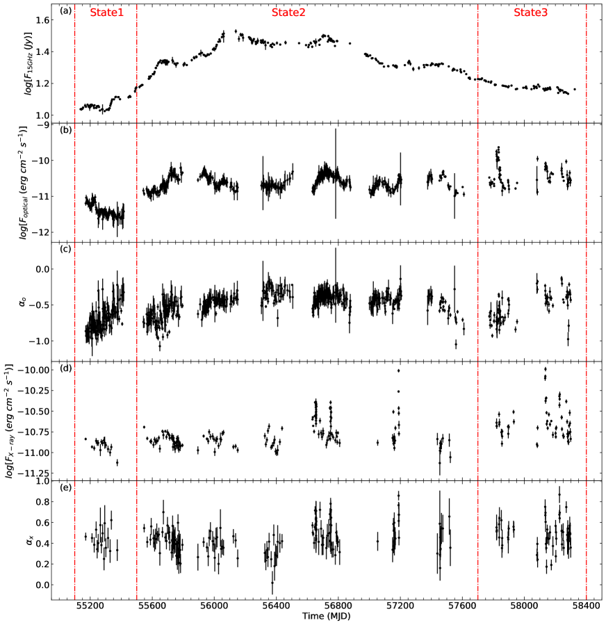
Figure 1: Multi-frequency light curves of 3C 279: (a): OVRO 15 GHz flux, (b): optical flux, (c): optical spectral index, (d): X-ray flux, and (e): X-ray spectral index. Vertical lines denote the time intervals for the states 1, 2, and 3 (see text), and the radio light curve is shown for reference.

For the XRT data, we first reprocess the data using xrtpipeline to produce cleaned event files. We then perform a spectral analysis using $R=R_{\rm in}-70^{\prime\prime}$ (with $R_{\rm in}$ varying depending on the degree of pile up) and $R=120-210^{\prime\prime}$ annular regions for the source and background, respectively. Note that photon pile-up occurred in some of the observations because of X-ray flares of 3C 279 (see also Larionov et al., 2020). In this case, we further inspect the event distribution and excise central regions affected by pile-up. The corresponding ancillary files are produced with xrtmkarf, and we use pre-computed redistribution matrix files (RMFs). We then fit the spectra with power-law models (tbabs*pow) holding $N_{\rm H}$ fixed at $2.2\times 10^{20}\rm\ cm^{-2}$ in XSPEC 12.9.1p to measure the source flux and produce the X-ray light curve. For the absorption model, we use vern cross section (Verner et al., 1996) and angr abundance (Anders & Grevesse, 1989). The fits are well acceptable with the typical $\chi^{2}$/dof=0.98. The resulting light curve is shown in Figure 1. Note that the Swift data used in this work were also analyzed and presented previously (e.g., Larionov et al., 2020; Prince, 2020), but we carry out more detailed ‘spectral’ studies in this paper.

2.2 Public catalog data

Swift UVOT provides optical data with reasonable quality but the cadence is insufficient for our studies; other data are necessary to cover the gaps. So we supplement the UVOT data with the public SMARTS- and Steward-catalog ones (Table 1; Smith et al., 2009; Bonning et al., 2012). We correct the optical data for Galactic extinction using $A_{\lambda}$ values found in NED (Schlafly & Finkbeiner, 2011), convert the magnitude into flux units (Bessell et al., 1998) and generate light curves. Note that some of the data were also presented in previous works (e.g., Paliya et al., 2015; Patiño-Álvarez et al., 2018; Larionov et al., 2020; Prince, 2020). We also use limited WISE observations ($\sim$$10^{13}$–$10^{14}$ Hz) here; these are not used for band spectral fits but for qualitative characterization of the SEDs. We also show the 15 GHz radio light curve obtained in the OVRO catalog (Richards et al., 2011) for reference (Fig. 1 a).

2.3 Time-series SED fitting

Although the narrow-band fluxes (i.e., each observation) provided important insights into blazar jets previously (e.g., Larionov et al., 2020; Prince, 2020), variability in the spectral shape cannot be studied in details with this approach. Since spectral shapes can be measured only with multi-frequency data, we combine the data together to construct time series of the spectra in the optical and X-ray bands.

For each of these bands, we combine the data within one day and construct SEDs in each of the wavebands. Using slightly different time bins (e.g., 2–3 days) does not significantly alter the results presented below. Note that when we compare quantities measured by Swift/XRT, we do not bin the data in time.

We fit the optical SEDs with power-law models $K(\nu/\nu_{0})^{\alpha}$, where $\nu_{0}$ is the pivot frequency taken to be the geometric mean of the fit band. We then measure the “logarithmic” flux ($F_{o}$; “flux” hereafter) and the spectral index ($\alpha_{o}$). In order to ensure that the observational data cover a wide frequency range ($\nu_{\rm min}$–$\nu_{\rm max}$) in the fits, we require that $\mathrm{log_{10}}(\nu_{\rm max}/\nu_{\rm min})$ is greater than 0.4 for the optical data. This requirement does not have large impact on the fits since the observations cover the fit band well. We verify that the models reasonably represent the SEDs by visual inspection.

The optical-band fits are formally unacceptable with reduced $\chi^{2}_{r}\gg 1$, meaning that the measurement uncertainties are underestimated and/or the simple power law is inadequate to fit the high-quality optical data; these will make the uncertainties on the model parameters incorrectly small. Although it is unclear what the poor fits should be ascribed to, we increase the measurement uncertainties by a factor so as to make the fit reduced $\chi_{r}^{2}=1$, which also increases the uncertainties in $F_{o}$ and $\alpha_{o}$. The results are displayed in Figure 1 (b and c). We note that the Pearson correlation coefficient and its Fisher transformation (Fisher, 1915) we use below take into account the scatter in the data (e.g., $F_{o}$ and $\alpha_{o}$ measurements), and so the measurement uncertainties are indirectly accounted for via the scatter. We verify the results obtained from the Fisher transformation using simulations when necessary (e.g., § 3.1).

The $0.3-10$ keV X-ray data are separately fit in XSPEC (see §2.1), and we measure the logarithmic flux ($F_{x}$) and derive the SED slope ($\alpha_{x}=2-\Gamma_{X}$). We present the results in Figure 1 (d and e). The WISE data cover three $\Delta T\approx 1$ day epochs at MJDs 55205, 55379, and 55567, and reveal that the optical continuum SED might curve downwards below $\sim$$10^{14}$ Hz at some epochs. The measured SED slopes are $-0.49\pm 0.03$/$-0.78\pm 0.13$, $-0.59\pm 0.03$/$-0.59\pm 0.12$, and $-0.72\pm 0.04$/$-0.77\pm 0.25$ for the WISE/optical data at MJDs 55205, 55379, and 55567, respectively.

3 Optical-to-X-ray variability of 3C 279

The light curves in Figure 1 show various phenomena at the observed frequencies. Long-term (years) and short-term (months) variabilities are clearly seen in the light curves. Some flares are observed only in one passband (e.g., the X-ray flare at MJD 56750 and the optical flare at MJD 57830), while some others are observed in multiple wavebands (e.g., $>$MJD 58000). It is hard to explain all these observational diversities with an emission scenario, and thus we focus on some of the features and a one-zone scenario here (see also Paliya et al., 2015; Larionov et al., 2020; Prince, 2020).

Table 2: Summary of correlations between the spectral properties

Band1	Band2	Property	$r_{p}$	Sig. ($\sigma_{F}$)	$N_{\rm pair}$
Full data (MJD 55100–58400):
Optical	Optical	$F_{o}$/$\alpha_{o}$	0.44	12.4	693
X-ray	X-ray	$F_{x}$/$\alpha_{x}$	0.65	12.0	239
Optical	X-ray	$F_{o}$/$F_{x}$	0.48	7.0	175
Optical	X-ray	$\alpha_{o}$/$\alpha_{x}$	$-$0.04	0.5	175
State 1 (MJD 55100–55500):
Optical	Optical	$F_{o}$/$\alpha_{o}$	$-$0.61	7.7	121
X-ray	X-ray	$F_{x}$/$\alpha_{x}$	0.14	0.5	16
Optical	X-ray	$F_{o}$/$F_{x}$	0.25	0.9	16
Optical	X-ray	$\alpha_{o}$/$\alpha_{x}$	0.04	0.1	16
State 2 (MJD 55500–57700):
Optical	Optical	$F_{o}$/$\alpha_{o}$	0.41	9.5	490
X-ray	X-ray	$F_{x}$/$\alpha_{x}$	0.72	11.5	166
Optical	X-ray	$F_{o}$/$F_{x}$	0.18	1.9	115
Optical	X-ray	$\alpha_{o}$/$\alpha_{x}$	$-$0.08	0.9	115
State 3 (MJD 57700–58400):
Optical	Optical	$F_{o}$/$\alpha_{o}$	0.07	0.6	82
X-ray	X-ray	$F_{x}$/$\alpha_{x}$	0.59	5.0	57
Optical	X-ray	$F_{o}$/$F_{x}$	0.54	3.9	44
Optical	X-ray	$\alpha_{o}$/$\alpha_{x}$	$-$0.07	0.5	44

In one-zone blazar emission models, the low-energy (optical) and the high-energy (X-ray to gamma-ray) radiations are related as they are assumed to share the emitting particles (i.e., electrons) in the same region (Abdo et al., 2010). Hence, correlation between optical and X-ray emission should exist, and we search the spectral data for such correlation. Here, we consider two spectral properties, flux ($F_{i}$) and spectral index ($\alpha_{i}$) in the optical ($i=o$) and X-ray bands ($i=x$), which makes up four correlations: one correlation between the spectral properties in each band (2 total) and two cross-band correlations for each property (2 total). Note that this approach is slightly different from the previous ones (e.g., Patiño-Álvarez et al., 2018; Beaklini et al., 2019; Larionov et al., 2020; Prince, 2020) in the sense that we use spectral indices as well and measure fluxes over broader bands which represent the continuum better.

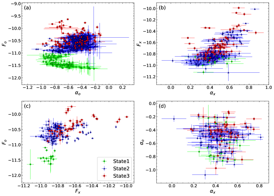
Figure 2: Scatter plots of the fit fluxes and spectral indices to show correlation within and across the wavebands. Correlations between $F_{i}$ and $\alpha_{i}$ within a waveband are shown in the top row: optical (a) and X-ray (b) bands. Cross-band correlations between the fit fluxes (c: $F_{o}$–$F_{x}$) and between the spectral indices (d: $\alpha_{o}$–$\alpha_{x}$) are displayed in the bottom row. Data points for each state are denoted in color: green circle for state 1, blue triangle for state 2 and red square for state 3.

3.1 Correlations within and across the wavebands

With the band-fit fluxes $F_{i}$’s and spectral indices $\alpha_{i}$’s that we measured (§2.3), we calculate the Pearson correlation coefficients ($r_{p}$) for the four pairs. The significance ($\sigma_{F}$) for the correlation is computed with the Fisher transformation. The results are summarized in Table 2 and scatter plots are shown in Figure 2. We verify that the significance estimated by the Fisher transformation well represents the null hypothesis probability using simulations; i.e., the chance probabilities for uncorrelated random samples (drawn from the normal distribution) to show the $r_{p}$ values in Table 2 correspond to $\sigma_{F}$’s estimated by the Fisher transformation.

In the single-band correlation study, we find very significant (e.g., $\geq$5$\sigma$) correlations in both bands (9-yr data). Although the optical flux $F_{o}$ and spectral index $\alpha_{o}$ show very significant correlation over the 9-yr period, it appears that there are two different “states” with dramatically different trends (i.e., negative and positive correlation) with a boundary at $F_{o}\approx-11$ (Fig. 2 a).

In the cross-band correlation study, we find significant correlations in $F_{o}$–$F_{x}$ (Fig. 2 c; see also Larionov et al., 2020). Like the $F_{o}$–$\alpha_{o}$ case (see above), the $F_{o}$–$F_{x}$ relation appears to form two groups depending on the $F_{o}$ values (Fig. 2 c). In addition, light curves after MJD 57700 show more frequent activities at high energies, differing from the earlier ones. We therefore group the data into three states: (1) MJD 55100–55500 with low optical flux, (2) MJD 55500–57700 with high optical flux and mild activity, and (3) MJD 57700–58400 with high optical flux and strong activity. Note that the time intervals for these states are similar to those used by Larionov et al. (2020) based on the $R$-band and gamma-ray flux relations, but are slightly different from theirs in that we do not use earlier data ($<$MJD 55100) and our state 3 includes their intervals 3 and 4.

The results for correlation studies in the states 1–3 are presented in Table 2. Note that the correlation in the $F_{o}$–$F_{x}$ relation (Fig. 2 c) in the full data set almost disappears in states 1 and 2, and is weaker in state 3, meaning that the correlation in the full data set is primarily between the states (inter-state) rather than within them (intra-state) and that the correlation in state 3 is an intra-state one. While the inter-state correlations can tell us about the state transition of the blazar, we focus on the intra-state ones here.

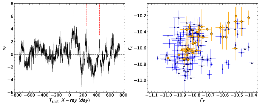
Figure 3: Left: significance plot for time-shift cross-band correlations between $F_{o}$ and $F_{x}$ in state 2. The x axis $T_{\rm shift}$ denotes the time shifts (1-day steps) and the shifted data with the positive values for X-ray lead. Negative y values mean anti-correlation. Red vertical lines mark 65 day, 255 day, and 445 day. Right: the corresponding scatter plot with $F_{x}$ shifted by 65 days (orange diamond). Unshifted data are overlaid in blue triangle for reference.

3.2 Time-shifted Correlations

Because the cross-band correlation may be more significant with a time delay if emission in one band lags (leads) the other, we perform the same correlation study by shifting the data in time. This is essentially the same as the discrete correlation function (DCF; Liodakis et al., 2018, for example) method except that our data are binned. We compare cross-band properties in pairs of the two wavebands by shifting one of the data in time and measure the correlation significance ($\sigma_{F}$) as a function of the time shift ($T_{\rm shift}$; 1-day step). The results are consistent with those in Table 2; the time-shifted plots corresponding to the significant (cross-band) ones in the table show a prominent peak at $T_{\rm shift}=0$.

However, we find that $F_{o}$ and $F_{x}$ in state 2, whose correlation was insignificant without a time shift (Table 2), show significant correlation when one of them is shifted in time ($r_{p}=0.73$ and $\sigma_{F}\approx$5.4 at $\sim$65 days; Fig. 3 left). As noted above (§ 3.1), $\sigma_{F}$ well represents the null hypothesis probability, and so the false alarm probability for the correlation with the 65-day delay (pre-trial $\sigma_{F}=5.4$) is $p=6\times 10^{-5}$ after considering 1,500 trials (i.e., $\sim$4$\sigma$ post-trial). A similar delay of 64 day found in MJD 56400–56850 by an independent study (Patiño-Álvarez et al., 2018) enhances the significance for the shifted correlation. In our new analysis of the data, we find that this delayed correlation in state 2 (MJD 55500–57700) is stronger over the whole period of the state than in a part of it (e.g., MJD 56400–56850; Patiño-Álvarez et al., 2018), implying that the delay persisted for a longer period (e.g., the whole state). We also note that Figure 3 seems to show a possible periodic trend with a period of 190 days (red vertical lines in the left panel). This is intriguing, but significance for the later peaks is low. The periodic trend in the figure might appear just by chance.

For the time-shifted $F_{o}$–$F_{x}$ correlation in state 2, we show the scatter plots of the shifted (orange diamond) and unshifted data (blue triangle) in Figure 3 right. In this state, there were several X-ray flares (Fig. 1) which can be seen as high-flux outliers in Figure 3 right. Since the source would have different emission properties during the flare periods from the low-flux quiescent ones (e.g., Hayashida et al., 2015), we check to see if the delayed correlation exists in the quiescent and flare periods separately. Because of the paucity of data points in flare, we investigate the quiescent periods only. We remove the high-flux outliers (i.e., taking $F_{x}\leq-10.75$), and compute $r_{p}$ and its significance which are $\approx 0.65$ and $\sigma_{F}\approx 4$, respectively.

4 Interpretation of the Spectral Correlation using a toy SED model

In this section, we present our explanation on the observed variabilities using a simple one-zone scenario.

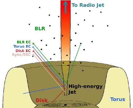
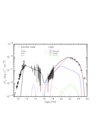
Figure 4: A schematic view of blazars’ emission components (left; not to scale), and a toy one-zone SED model and time-averaged SED data (right). The optical and X-ray data points are measured in this work (collected over $\sim$9 years), and the error bars on the data points are the standard deviation of the measurements. The radio and gamma-ray points are taken from the vizier catalog and the 4FGL catalog (8-year average), respectively. The summed model is displayed with a solid black line and each model component is denoted in color. Note that the synchrotron component (brown dotted) is shown without SSA to be compared to a model with SSA (black solid).

4.1 A Toy SED model

In order to explain the spectral correlations we found above, we construct a toy one-zone SED model using a leptonic synchro-Compton scenario (Fig. 4; see also Sahayanathan & Godambe, 2012; Dermer et al., 2014; Paliya et al., 2015, for example). In this work, we do not attempt to strictly match the highly-variable observational SEDs of 3C 279 with the toy model, but it is constructed so as to capture the main features of the SED and the relevant ingredients in blazar emission for our investigation of the spectral correlations; the figure is intended to be used only to guide eyes. The model and time-averaged SED data are shown in Figure 4, where the error bars on the optical and X-ray data points are standard deviation of the 9-yr flux measurements at the observed frequencies. Note that the gamma-ray SED is obtained from the 4FGL catalog (Abdollahi et al., 2020) and is a mission-averaged one, and the radio data are taken from the vizier photometry webpage.

In this model, the optical SED is explained with the synchrotron radiation (brown dotted) of a broken power-law electron distribution ($dN_{e}/d\gamma_{e}\propto\gamma_{e}^{-p_{1}}$ with $p_{1}=3.3$ if $\gamma_{e}\geq 50$ and $p_{1}=2.3$ otherwise) and weak disk emission at the high-frequency end (red dotted). The spectral indices for the electron distribution are chosen so as to match the optical SED displayed in Figure 4 right and are similar to those expected in shock acceleration theories (e.g., Jones & Ellison, 1991) and radiative cooling. The disk emission is computed following the standard Shakura-Sunyaev model for $M_{\rm BH}=5\times 10^{8}M_{\odot}$ (Shakura & Sunyaev, 1973). Emissions of a torus and a broad line region (BLR) are included as blackbody radiation (e.g., Joshi et al., 2014); our investigation below does not strongly depend on the exact emission properties of these components (e.g., the emission frequency and spectral shape). We also show the SSC component (brown dashed) for reference but it may be even lower; given the observed shape of the average X-ray SED, this component cannot be significant. In the X-ray band, the emission is assumed to be produced by EC of torus (blue dashed) and disk photons (red dashed). Although the BLR EC is much weaker than the disk EC in our model, the converse is also possible if the jet locates closer to BLR/torus (e.g., Dermer, 1995); BLR emitting at slightly lower frequencies may replace the disk EC in the model.

Variability in this scenario can occur for various reasons: changes in internal conditions of the jet (e.g., particle spectrum $N_{e}$, magnetic-field strength $B$, the Doppler factor $\delta$), location of the jet (i.e., EC efficiency), and change in the external seeds for EC (e.g., variable external emission $u_{\rm ext}$). In the model, the frequencies and fluxes of the low-energy (synchrotron in the optical band) and the high-energy (EC in the X-ray to gamma-ray band) SED humps are related to the jet properties as in the following (e.g., Dermer, 1995; An & Romani, 2017):

$$\nu_{\rm SY} \propto \delta B\gamma_{e}^{2},\mathrm{\ }\ \ \ \ \ \ F_{\rm SY}\propto B^{(1+p_{1})/2}\delta^{(5+p_{1})/2}$$

$$\nu_{\rm EC} \propto \delta^{2}\gamma_{e}^{2}\nu_{\rm ext},\mathrm{\ }\ \ F_{\rm EC}\propto\delta^{3+p_{1}}u_{\rm ext},$$

where $\nu_{\rm SY,EC}$ and $F_{\rm SY,EC}$ are the observed (synchrotron and EC) emission frequency and flux, and $\nu_{\rm ext}$ and $u_{\rm ext}$ are the emission frequency and flux of the external seeds for EC. Given the relatively straight power-law shape of the optical spectrum of 3C 279 (Fig. 4), the optical spectral index would not change much by $\delta$ and/or $B$ (shifts of the SED) unless they vary a lot (e.g., orders of magnitude), in which case the flux would change even more. So variation of the optical spectral index ($\alpha_{o}$) would be likely due to changes of the particle spectrum $N_{e}$ with small contribution from $\delta$ and/or $B$.

Note that this model accounts only for the high-energy jet in which radio emission is highly suppressed by SSA (black solid vs. brown dotted lines). The radio emission is assumed to be produced in a separate parsec-scale ‘radio’ jet.

4.2 State 1: MJD 55100–55500

In state 1 during which the optical flux is low, $F_{o}$–$\alpha_{o}$ shows negative correlation. No cross-band correlation is found. Although the changes of $F_{o}$ and $\alpha_{o}$ may occur for various reasons as we noted above, the ‘negative’ $F_{o}$–$\alpha_{o}$ correlation may suggest that the change is stronger at low frequencies (i.e., soft), and can occur if $N_{e}$ varies in the jet region.

A change of $N_{e}$ would necessarily result in a corresponding change in the X-ray SED in one-zone scenarios; the optical and X-ray light curves (Fig. 1) show a hint of a correlated flux change (both drop with time), but the correlation is not significantly detected, perhaps because of the low statistics (16 pairs in this state). We verify this using simulations performed with correlated random samples and with the measured data; only $\leq$1$\sigma$ detection of $r_{p}\approx 0.25$ correlation (e.g., $F_{o}$/$F_{x}$ in Table 2) is possible with 16 pairs. Note that gamma-ray flux also drops in this state (e.g., Larionov et al., 2020). These imply that the soft-spectrum particles ($N_{e}$) were being removed from the high-energy emission region in this state. We may speculate that these particles move to the radio jets, thereby producing radio emission; the radio brightening in state 1 (Fig. 1) may support our speculation although the radio activity may be irrelevant to the optical one and was produced by a shock propagating in the radio jet (Hovatta et al., 2008) and/or independent changes in conditions in the radio jet: $\delta$, $B$, and/or injection of particles.

4.3 State 2: MJD 55500–57700

In this state, properties within the bands are all positively correlated. In particular, the $F_{x}$-$\alpha_{x}$ correlation can give us strong constraints on the emission mechanism of the high-energy ($\geq$X-rays) radiation. This state overlaps very well with interval 2 of Larionov et al. (2020) in which the $R$-band ($F_{R}$) and gamma-ray ($F_{\gamma}$) flux relation of $F_{\gamma}\propto F_{R}^{7.7}$ is found. We note that the significant $F_{o}$–$\alpha_{o}$ correlation is primarily due to grouping of low-flux (e.g., $F_{o}\leq-10.8$) and high-flux points (blue points in Fig. 2 a); ignoring the low-flux ones reduces the significance rapidly. This indicates that state 2 may be further split, but the low-flux points do not localize in time. Therefore, we do not further split this state and regard that the $F_{o}$–$\alpha_{o}$ correlation is less significant (e.g., $\sim$3.8$\sigma$ for $F_{o}\geq-10.8$).

Aside from the radio variability, observational properties in this state are that (1) $F_{\gamma}\propto F_{R}^{7.7}$, (2) $F_{x}$ and $\alpha_{x}$ show “positively” correlated variability, implying that the disk EC varies more than the torus EC does, (3) $F_{x}$ leads $F_{o}$ by $\sim$65 days (Fig. 3 left), and (4) variability in the optical spectral index implies $N_{e}$ variation. Because $F_{\rm EC}/F_{\rm SY}\propto\delta^{\frac{1+p_{1}}{2}}u_{\rm ext}/B^{\frac{1+p_{1}}{2}}$, changes of $\delta$, $B$ (by a factor of $\leq 3$), and/or $u_{\rm ext}$ can explain (1). However, (2) is hard to be produced by the internal properties $\delta$ and $B$ (e.g., $\alpha_{x}$ variability), and therefore we can conclude that $u_{\rm ext}$ is the primary source of the X-ray and hence gamma-ray variability. Furthermore, (3) cannot be explained by changes in the internal properties of the jet either because these will change the X-ray emission instantaneously (i.e., no delay).

Although the enhanced X-ray and gamma-ray emission should be driven by an increase in the external disk seed photons ($u_{\rm ext}$), the ‘delayed’ optical emission (3) cannot be produced by the external sources themselves (e.g., disk) whose emission is much weaker than the synchrotron continuum (e.g., Fig. 4) and will ‘lead’ the reprocessed (upscattered) X-rays. Therefore, we speculate that the disk (external) activity responsible for (1) and (2) might enhance the optical continuum emission $\sim$65 days later by synchrotron radiation in the ‘jet’; perhaps enhanced injection from the disk to the jet is responsible for this.

The ‘delayed’ optical variability (synchrotron) is natural in this scenario as $N_{e}$ would vary by injection, but then the X-ray flux should also increase simultaneously by EC of the same $N_{e}$. Then $F_{x}$–$F_{o}$ correlation with no delay in addition to the 65-day shifted one is expected but we do not see correlation without a delay (e.g., Fig 3 left). Perhaps, $F_{x}$ variability induced by the injection into the jet ($N_{e}$) is swamped by the 65-day earlier disk EC activity ($u_{\rm ext}$). Alternatively, the ‘delayed’ optical continuum variability (synchrotron in the jet) may be driven mainly by changes of $B$ which affect $F_{o}$ but not $F_{x}$. Indeed, the change of the optical flux (a factor of $\sim$4) is larger than that of the X-ray one (a factor of $\sim$2 ignoring large X-ray flux points $F_{x}\geq-10.8$ induced by flares; Fig. 3 right), suggesting that $B$ may be the dominant factor (over $N_{e}$) for the delayed optical variability.

4.4 State 3: MJD 57700–58400

This state shows rapid and large variability in the high-energy band, suggesting that 3C 279 was active. Since our spectral data do not cover this time interval well, highly significant (e.g., $\geq$5$\sigma$) correlation is found only between $F_{x}$ and $\alpha_{x}$ (Table 2 and red square points in Fig. 2 b), implying that the disk EC is still variable. If the disk EC is the main driver of the high-energy variability, a strong $F_{\gamma}$–$F_{R}$ trend as in state 2 is expected. However, Larionov et al. (2020) reported a weaker $F_{\gamma}\propto F_{R}^{1.9}$ trend in this state. This implies that the optical continuum emission also varied with the X-ray one; fairly significant 4-$\sigma$ $F_{o}$–$F_{x}$ correlation (Table 2) also suggests this (see also Prince, 2020).

Provided that the optical flux is dominated by the synchrotron continuum radiation, it is likely that changes of $N_{e}$ and $\delta$ are the main driver of the variability in this state. Assuming that $B$ is constant and $p_{1}\approx 2.3$, we find $F_{\rm EC}\propto F_{\rm SY}^{1.5}$, similar to $F_{\gamma}\propto F_{R}^{1.9}$ trend. Hence the variability in this state can be explained by changes of $\delta$ and $N_{e}$ (spectral shape change in the optical band) with relatively weak disk EC variability ($F_{x}$–$\alpha_{x}$ correlation).

5 Summary and Conclusion

We investigated multi-frequency variability in the emission of the blazar 3C 279 using Swift UVOT/XRT, and various catalog data. We produced multi-band spectra and analyzed them in order to infer physical properties and emission mechanisms of the jet. We constructed time-resolved SEDs in the two wavebands, carried out spectral correlation studies, and found several significant correlations between the spectral properties within and across the wavebands. Note that variability in 3C 279 emission is much more complicated and may differ in each flare activity (e.g., Paliya et al., 2015; Hayashida et al., 2015), and that the correlations we found represent the overall properties of the 3C 279 jet.

In these spectral studies, we found that the $F_{o}$–$\alpha_{o}$ correlation exhibits a strong inversion, and therefore we split the data into three states based on the $F_{o}$–$\alpha_{o}$ correlation and activity in the light curves. We then investigated correlation properties in each state and interpret the results using a one-zone synchro-Compton scenario. Below are the summary:

• State 1: the $F_{o}$–$\alpha_{o}$ anti-correlation and a mild flux drop in the optical to gamma-ray band with time suggest that soft-spectrum particles ($N_{e}$) are lost from the high-energy jet.

• State 2: the $F_{\gamma}\propto F_{R}^{7.7}$ relation (Larionov et al., 2020) and $F_{x}$–$\alpha_{x}$ correlation imply that the disk-EC emission is variable due to some activity in the disk. Then the $\sim$65-day lag of $F_{o}$ with respect to $F_{x}$ and variability in the optical spectral index suggest that the activity in the disk might inject particles $N_{e}$ and $B$ into the high-energy jet on a time scale of $\sim$65 days.

• State 3: $F_{x}$–$\alpha_{x}$ correlation again implies variability in the disk EC, and the $F_{o}$–$F_{x}$ correlation and the $F_{\gamma}\propto F_{R}^{1.9}$ relation suggest that it is $\delta$ that mainly drives the variability in this state with some contribution of $N_{e}$ and disk EC.

If it is the disk EC emission that drives the variability at X-rays in state 2 as we argued above, a 65-day delay of the optical emission with respect to the gamma-ray one is also expected in state 2 and was seen in the earlier part of the state (Patiño-Álvarez et al., 2018). This implies that the emission mechanisms for X-rays and gamma rays are the same as in our SED model (Fig. 4).

It is interesting to note that the near “quiescent” state (state 1), a short period ($\sim$400 days) after large radio activity (e.g., Chatterjee et al., 2008), is followed by active states (states 2 and 3) in which injection of $N_{e}$ and changes of $B$/$\delta$ occur. The time interval is coincident with new long-term radio activity, and it is worth investigating whether and how the high-energy ($\geq$optical) states are related to the radio activity. Investigations of high-energy data taken during previous and future long-term radio activity may be very intriguing.

Because 3C 279 is very bright and frequently observed, high-quality multi-band data exist. Using only small part of the observational data and a one-zone SED scenario, we were able to suggest that the emission mechanism for the high-energy SED hump is the tours and disk EC, and explore causes of the spectral variability. Although the one-zone model can explain the results obtained in this work, the source exhibits enormously diverse spectral variability that cannot be explained with the model. More data (e.g., time-varying broadband SEDs) and improved SED models can certainly provide very useful information. In this regard, we acknowledge that our interpretation is speculative rather than definitive. Further comprehensive data analyses (e.g., including polarization and gamma-ray emission; Abdo et al., 2010) and theoretical studies (e.g., magnetohydrodynamic simulations and multi-zone SED models) are warranted to advance our knowledge on 3C 279, and blazars in general.

References

- Abdo et al. (2010) Abdo, A. A., Ackermann, M., Ajello, M., et al. 2010, Nature, 463, 919
- Abdollahi et al. (2020) Abdollahi, S., Acero, F., Ackermann, M., et al. 2020, ApJS, 247, 33
- Ackermann et al. (2016) Ackermann, M., Ajello, M., An, H., et al. 2016, ApJ, 820, 72
- An & Romani (2017) An, H., & Romani, R. W. 2017, ApJ, 838, 145
- An & Romani (2018) —. 2018, ApJ, 856, 105
- Anders & Grevesse (1989) Anders, E., & Grevesse, N. 1989, Geochim. Cosmochim. Acta, 53, 197
- Arnaud (1996) Arnaud, K. A. 1996, in Astronomical Society of the Pacific Conference Series, Vol. 101, Astronomical Data Analysis Software and Systems V, ed. G. H. Jacoby & J. Barnes, 17
- Beaklini et al. (2019) Beaklini, P. P. B., Dominici, T. P., Abraham, Z., & Motter, J. C. 2019, A&A, 626, A78
- Bessell et al. (1998) Bessell, M. S., Castelli, F., & Plez, B. 1998, A&A, 333, 231
- Blandford & Znajek (1977) Blandford, R. D., & Znajek, R. L. 1977, MNRAS, 179, 433
- Bonning et al. (2012) Bonning, E., Urry, C. M., Bailyn, C., et al. 2012, ApJ, 756, 13
- Bottacini et al. (2016) Bottacini, E., Böttcher, M., Pian, E., & Collmar, W. 2016, ApJ, 832, 17
- Böttcher et al. (2013) Böttcher, M., Reimer, A., Sweeney, K., & Prakash, A. 2013, ApJ, 768, 54
- Chatterjee et al. (2008) Chatterjee, R., Jorstad, S. G., Marscher, A. P., et al. 2008, ApJ, 689, 79
- Dermer (1995) Dermer, C. D. 1995, ApJ, 446, L63
- Dermer et al. (2014) Dermer, C. D., Cerruti, M., Lott, B., Boisson, C., & Zech, A. 2014, ApJ, 782, 82
- Fisher (1915) Fisher, R. A. 1915, Biometrika, 10, 507
- H. E. S. S. Collaboration et al. (2013) H. E. S. S. Collaboration, Abramowski, A., Acero, F., et al. 2013, A&A, 550, A4
- Hayashida et al. (2015) Hayashida, M., Nalewajko, K., Madejski, G. M., et al. 2015, ApJ, 807, 79
- Hovatta et al. (2008) Hovatta, T., Nieppola, E., Tornikoski, M., et al. 2008, A&A, 485, 51
- Jones & Ellison (1991) Jones, F. C., & Ellison, D. C. 1991, Space Sci. Rev., 58, 259
- Joshi et al. (2014) Joshi, M., Marscher, A. P., & Böttcher, M. 2014, ApJ, 785, 132
- Larionov et al. (2020) Larionov, V. M., Jorstad, S. G., Marscher, A. P., et al. 2020, MNRAS, 492, 3829
- Liodakis et al. (2018) Liodakis, I., Romani, R. W., Filippenko, A. V., et al. 2018, MNRAS, 480, 5517
- MacDonald et al. (2015) MacDonald, N. R., Marscher, A. P., Jorstad, S. G., & Joshi, M. 2015, ApJ, 804, 111
- Marziani et al. (1996) Marziani, P., Sulentic, J. W., Dultzin-Hacyan, D., Calvani, M., & Moles, M. 1996, ApJS, 104, 37
- Paliya et al. (2015) Paliya, V. S., Sahayanathan, S., & Stalin, C. S. 2015, ApJ, 803, 15
- Patiño-Álvarez et al. (2018) Patiño-Álvarez, V. M., Fernandes, S., Chavushyan, V., et al. 2018, MNRAS, 479, 2037
- Prince (2020) Prince, R. 2020, ApJ, 890, 164
- Richards et al. (2011) Richards, J. L., Max-Moerbeck, W., Pavlidou, V., et al. 2011, ApJS, 194, 29
- Rodrigues et al. (2018) Rodrigues, X., Fedynitch, A., Gao, S., Boncioli, D., & Winter, W. 2018, ApJ, 854, 54
- Romani et al. (2004) Romani, R. W., Sowards-Emmerd, D., Greenhill, L., & Michelson, P. 2004, ApJ, 610, L9
- Sahayanathan & Godambe (2012) Sahayanathan, S., & Godambe, S. 2012, MNRAS, 419, 1660
- Schlafly & Finkbeiner (2011) Schlafly, E. F., & Finkbeiner, D. P. 2011, ApJ, 737, 103
- Shakura & Sunyaev (1973) Shakura, N. I., & Sunyaev, R. A. 1973, A&A, 500, 33
- Smith et al. (2009) Smith, P. S., Montiel, E., Rightley, S., et al. 2009, arXiv e-prints, arXiv:0912.3621
- Urry & Padovani (1995) Urry, C. M., & Padovani, P. 1995, PASP, 107, 803
- Verner et al. (1996) Verner, D. A., Ferland, G. J., Korista, K. T., & Yakovlev, D. G. 1996, ApJ, 465, 487